New formulations and branch-and-cut procedures
for the longest induced path problem
Abstract
Given an undirected graph , the longest induced path problem (LIPP) consists of obtaining a maximum cardinality subset such that induces a simple path in .
In this paper, we propose two new formulations with an exponential number of constraints for the problem, together with effective branch-and-cut procedures for its solution. While the first formulation (cec) is based on constraints that explicitly eliminate cycles, the second one (cut) ensures connectivity via cutset constraints.
We compare, both theoretically and experimentally, the newly proposed approaches with a state-of-the-art formulation recently proposed in the literature.
More specifically, we show that the polyhedra defined by formulation cut and that of the formulation available in the literature are the same. Besides, we show that these two formulations are stronger in theory than cec.
We also propose a new branch-and-cut procedure using the new formulations.
Computational experiments show that the newly proposed formulation cec, although less strong from a theoretical point of view, is the best performing approach as it can solve all but one of the 1065 benchmark instances used in the literature within the given time limit. In addition, our newly proposed approaches outperform the state-of-the-art formulation when it comes to the median times to solve the instances to optimality.
Furthermore, we perform extended computational experiments considering more challenging and hard-to-solve larger instances and evaluate the impacts on the results when offering initial feasible solutions (warm starts) to the formulations.
Keywords: combinatorial optimization, integer programming, longest induced path, maximum induced subgraphs, maximum cardinality.
1 Introduction
Given a simple undirected graph , the longest induced path problem (LIPP), also known as the maximum induced path problem, consists of obtaining a maximum cardinality subset of vertices inducing a simple path. More formally, denote by the graph induced in by , whose set of edges is formed by all the edges in whose extremities belong to , namely, . LIPP consists of obtaining a maximum cardinality subset inducing a simple path . The problem is known to be NP-hard as its decision version is NP-complete Garey & Johnson (1979). Figure 1 exemplifies an input graph and one of its longest induced paths.
LIPP encounters applications in both practical and more graph theoretical situations. Obtaining the longest induced paths in hypercube graphs is known as the snake-in-the-box problem and has applications in error-checking codes, communications, and data storage Kautz (1958); Yehezkeally & Schwartz (2012); Hood et al. (2015). Given a graph and two predefined vertices , the detour distance between and is defined as the length of the longest induced path between them Chartrand et al. (1993). In this context, LIPP finds applicability in the evaluation of worst case transmission times in large communication and neural networks Gavril (2002). Additionally, it is also applicable to the analysis of social networks as it extends the concept of diameter of a graph, which is given by the longest of its shortest paths Matsypura et al. (2019). Furthermore, the existence of long induced paths plays an important role in the characterization of properties for several problems in graph theory Lozin & Rautenbach (2003); Golovach et al. (2014); Bonomo et al. (2018); Chudnovsky et al. (2019); Jaffke et al. (2020).
Although LIPP is NP-hard in general, there are several classes of graphs for which it can be solved in polynomial time Gavril (2002); Kratsch et al. (2003); Ishizeki et al. (2008); Jaffke et al. (2020). However, to the best of our knowledge, approaches for solving general instances of the problem were only proposed very recently. Matsypura et al. (2019) presented three compact integer programming (IP) formulations and an exact iterative IP-based algorithm using their IP formulations. The authors also presented a randomized heuristic to tackle larger instances of the problem. Bökler et al. (2020); Bökler et al. (2020) described branch-and-cut approaches based on IP formulations using cutset (or generalized subtour elimination) constraints and clique inequalities. The authors showed that the proposed formulations provide stronger linear relaxation bounds than those presented in Matsypura et al. (2019). Furthermore, computational experiments demonstrated the superiority of the new formulations in terms of the number of instances solved to optimality and the median times for solving them. Marzo & Ribeiro (2021) proposed an exact backtracking algorithm, based on which they also derived a heuristic approach.
In addition, several problems which are somehow related to the longest induced path problem have been tackled using integer programming approaches in the literature. Ljubić et al. (2006) and Costa et al. (2009) presented integer programming formulations and branch-and-cut methods for Steiner tree problems. The problem of obtaining the longest induced simple cycle of a graph was considered in Lucena et al. (2013). Formulations for the maximum weighted connected subgraph problem were proposed in Álvarez-Miranda et al. (2013), and Rehfeldt & Koch (2019). Agra et al. (2017) analyzed exact approaches for finding maximum -regular induced subgraphs of a graph. Melo et al. (2021) considered the maximum weighted induced forest problem in the context of solving the minimum weighted feedback vertex set problem. Melo & Ribeiro (2021) proposed new IP formulations for the maximum weighted induced forest problem and showed how to adapt their approaches to find maximum weighted induced trees.
In the same line of the recent works of Matsypura et al. (2019), Bökler et al. (2020); Bökler et al. (2020), and Marzo & Ribeiro (2021), we consider the longest induced path problem for general graphs. We propose two new formulations with exponential numbers of constraints. We perform a theoretical comparison regarding the polyhedra defined by these formulations and that of a state-of-the-art formulation available in the literature Bökler et al. (2020). We also propose an effective branch-and-cut approach for the problem which, based on the characteristics of the instance, either adds a priori to the formulation the clique inequalities for all the maximal cliques in the graph, or applies a cutting-plane heuristic to separate such inequalities. Extensive computational experiments are conducted, highlighting the superiority of our approaches when compared to a state-of-the-art formulation in terms of both the number of instances solved to optimality and the median times to solve them.
The remainder of the paper is organized as follows. Section 2 describes the newly proposed formulations. Section 3 presents the computational experiments, where implementation details of the branch-and-cut approach are also given. Concluding remarks are discussed in Section 4. For the sake of completeness, the state-of-the-art formulation proposed in Bökler et al. (2020) is presented in Appendix A. A theoretical comparison of the polyhedra defined by the different, existing and new, problem formulations is presented in Appendix B. A theoretical analysis of the different clique inequalities is presented in Appendix C.
2 New integer programming formulations
In this section, we propose two new formulations with an exponential number of constraints for the longest induced path problem (LIPP). We also describe the clique inequalities available for problems related to encountering induced subgraphs. Both formulations are undirected and consider a slightly modified graph constructed as follows, as Bökler et al. (2020) also did. Given the graph , we build with and . The goal of the dummy vertex is to be linked to both extremities of the induced path , with . In the remainder of the paper, let be the set of edges in with both extremities in , and be the set of edges in with an extremity in and another one in .
2.1 Formulation with explicit cycle elimination constraints
In order to formulate LIPP as an integer program, define the binary variable to be equal to one if the vertex belongs to the solution, zero otherwise. Besides, consider the binary variable to be equal to one if edge is in the solution, zero otherwise. Let denote the family of all cycles in the graph . The formulation with explicit cycle elimination constraints can be defined as
| (1) | |||||
| (2) | |||||
| (3) | |||||
| (4) | |||||
| (5) | |||||
| (6) | |||||
| (7) | |||||
| (8) | |||||
The objective function (1) maximizes the number of vertices in the induced path. Constraints (2) guarantee that each selected vertex has degree two. Constraint (3) ensures exactly two edges are adjacent to the dummy vertex. Constraints (4) force the induced subgraph to be acyclic. Note that there is an exponential number of such constraints, one for each cycle in the graph. Constraints (5) and (6) ensure the path is induced. Constraints (7) and (8) determine, respectively, the integrality of the and variables.
Note that, similarly to Bökler et al. (2020), the formulation assumes . We remark, though, that such assumption is not restrictive, as obtaining the optimal solution for a graph without any edges is straightforward. An alternative way that could include the trivial graph as a feasible input would be to insert an additional dummy vertex to the transformed graph and, instead of closing a cycle with both extremities of the induced path, one would build a path between the two dummy vertices.
2.2 Formulation with cutset constraints
The undirected cutset formulation is similar to that with explicit cycle elimination constraints, with the difference that it guarantees the elimination of cycles using cutset constraints. Using the same variables defined in Subsection 2.1, it can be cast as
| (9) | |||||
Constraints (9) guarantee the solution to be acyclic in by ensuring connectivity. To be more specific, given a partition , with vertex , the constraint enforces at least two edges in the cut to be in the solution whenever .
Note that an alternative well-known approach for ensuring connectivity, which is known to be equivalent to the use of cutset inequalities, is the employment of generalized subtour elimination constraints Goemans & Myung (1993); Bökler et al. (2020). This means that an equivalent way to ensure (9) is via
| (10) |
Constraints (10) guarantee that for a given subset of vertices, the number of edges connecting them is at most the number of selected vertices minus one (whenever there is at least one selected edge from ).
2.3 Clique inequalities
A clique in a graph is a subset of its vertices which are all pairwise adjacent. Consider to be the family of all cliques in the graph . Bökler et al. (2020); Bökler et al. (2020) described the clique inequalities using the edge variables as
| (11) |
Inequalities (11) enforce the number of edges connecting vertices in a clique to be at most one.
On the other hand, clique inequalities can also be modeled using the variables corresponding to the vertices Brunetta et al. (2000); Melo & Ribeiro (2021), resulting in
| (12) |
Inequalities (12) ensure that at most two vertices in a clique are selected.
2.4 Theoretical analysis of the formulations and clique inequalities
We provide a theoretical comparison regarding the polyhedra defined by formulations cec, cut, and BCWWy Bökler et al. (2020); Bökler et al. (2020) in Appendix B. Namely, we show that the polyhedra defined by cut and BCWWy are equivalent. We also prove that the polyhedra determined by cut and BCWWy are strictly contained in that defined by cec. For completeness, BCWWy is described in Appendix A.
3 Computational experiments
In this section, we report the computational experiments assessing the performance of the newly proposed formulations. The experiments were carried out on a machine running under Ubuntu, with an Intel(R) Core(TM) i7-8700 Hexa-Core 3.20 GHz and 16 GB of RAM. The formulations were coded in Julia v1.4.2, using JuMP v0.18.6. Furthermore, the formulations were solved using Gurobi 9.0.2.
We considered in our experiments the instances proposed for the longest induced path problem in Matsypura et al. (2019) and Bökler et al. (2020), also used by Marzo & Ribeiro (2021). These instances can be obtained from Bökler et al. (2019), where additional details can be encountered. They are grouped into four sets, which are: RWC, MG, BAS, and BAL. RWC is composed of 22 real-world networks corresponding to communication and social networks of companies, characters in books, as well as transportation, biological and technical networks. MG corresponds to The Movie Galaxy dataset and contains 773 graphs associated to social networks of movie characters Kaminski et al. (2018). BAS and BAL were generated by Bökler et al. (2020) using the Barabási-Albert probabilistic model for scale-free networks Barabási & Albert (1999) in an attempt to recreate those used in Matsypura et al. (2019). BAS is composed of 120 graphs divided into four subsets with , where , having 30 instances each. BAL is composed of 150 graphs with 100 vertices divided into five subsets with , each of them containing 30 instances.
3.1 Tested approaches
The following approaches were considered in our experiments:
- -
cec: the formulation with explicit cycle elimination constraints, described in Section 2.1;
- -
cut: the formulation with cutset constraints, described in Section 2.2;
- -
: best performing formulation described in Bökler et al. (2020) (see Appendix A);
- -
: formulation described in Bökler et al. (2020) corresponding to without the clique inequalities (see Appendix A).
Note that we do not explicitly consider in our experiments the approaches of Matsypura et al. (2019), as they were already shown not to be as effective in general as those proposed in Bökler et al. (2020).
The reported values for and are those in Bökler et al. (2020); Bökler et al. (2020). We observe that we implemented their formulations and executed our implementations in our own computational environment. However, although our implementation showed a similar performance for the small and medium instances in the original benchmark set, its results were outperformed by those reported by the authors for the larger instances. Thus, Table 1 compares the computational resources involved in the experiments based on the benchmarks in PassMark (2021) to evaluate the performance of the formulations.
| Benchmarks | Intel Core i7-8700 | Intel Xeon Gold 6134 |
|---|---|---|
| Clock speed (GHz) | 3.2 | 3.2 |
| Turbo speed (GHz) | Up to 4.6 | Up to 3.7 |
| CPU single thread rating | 2,681 | 2,251 |
| CPU mark rating | 13,090 | 16,513 |
3.2 Implementation details and parameter settings
We report in this section some relevant implementation issues.
(A) Separation of cycle constraints:
the separation of the cycle constraints (4) for formulation cec is performed based on the approach described in Melo & Ribeiro (2021). It receives as input a separation graph induced by the vertices corresponding to the variables assuming a nonzero value in the solution (which can be either a fractional solution corresponding to the linear relaxation or an integer solution). More specifically, , where represents the value assumed by variable in the solution. The separation of violated inequalities for integer solutions is performed using the well-known depth-first search algorithm (DFS) Cormen et al. (2009) in . More specifically, for every back edge traversed during the DFS, the corresponding cycle is stored. The separation procedure adds to the formulation all the cycles encountered during the execution of DFS. On the other hand, the separation for fractional solutions is performed heuristically. It uses an alternative DFS with certain greedy components in by considering the vertices to be visited in non-increasing order of their associated values. Whenever a back edge is traversed during the search, the algorithm checks if such cycle violates constraints (4). In case that happens, it is stored. At the end of the execution of this alternative DFS, the separation procedure adds to the formulation all the violated inequalities which were encountered during the procedure.
(B) Separation of cutset constraints:
the separation of the cutset constraints (9) for formulation cut also takes as input. The separation of violated inequalities for integer solutions is performed with a small variation of the well-known breadth-first search algorithm (BFS) Cormen et al. (2009) in . The algorithm starts at the dummy vertex and defines the part of the partition of as the vertices which could be reached from . In what follows, for each vertex in the algorithm stores the corresponding violated inequality. At the end of the execution of the algorithm, all the encountered violated inequalities are added to the formulation. Separation for fractional solutions is performed exactly using maximum flows (minimum cuts), following the approach of Magnanti & Wolsey (1995). Namely, the approach builds a directed graph based on the solution in which the capacities of the arcs are defined by the values assumed by the variables. Thus, a maximum flow problem is solved from to each . A violated constraint (9) is stored whenever it is encountered. At the end of the execution of the algorithm, all the obtained violated inequalities are inserted into the formulation.
(C) Separation of clique inequalities:
the separation of clique inequalities (12) for formulations cec and cut also takes the separation graph as input. It uses the heuristic approach described in Melo & Ribeiro (2021), which works as follows. Firstly, the vertices in are sorted in non-increasing order of their corresponding values. In case of ties, they are considered in non-increasing order of their degree in . Next, a vertex adjacent to all others that were already chosen is greedily chosen to compose the clique under construction. These steps are repeated while a maximal clique in was not yet obtained. Whenever a violated inequality is obtained for a maximal clique in , the approach attempts to lift such inequality by possibly adding new vertices that were not in the separation graph to get a maximal clique in the original graph . The selection of vertices to lift the inequality uses a similar greedy idea, but it only considers their degrees.
(D) A priori addition of clique inequalities:
in certain situations, we also consider adding a priori to the formulation the clique inequalities corresponding to all the maximal cliques in the graph. The enumeration of maximal cliques can be performed based on the algorithm of Bron and Kerbosch Bron & Kerbosch (1973); Tomita et al. (2006). Although the maximum number of such cliques can be exponential Moon & Moser (1965), it was observed in Bökler et al. (2020) that, for most of the benchmark instances, the number of maximal cliques was rather reasonably tractable.
(E) Settings and further details:
whenever the number of maximal cliques with at least three vertices do not exceed a parameter , all the corresponding clique inequalities are added a priori to the formulation. Otherwise, the separation of clique inequalities is employed. Based on preliminary tests to check the tractability of larger formulations, in our experiments, was set to 500. All the separation procedures were implemented as callbacks in the MIP solver. The separations for fractional solutions were configured to be executed only at the root node in an attempt not to overload the formulation with inequalities generated throughout the search tree. The MIP solver was executed using the standard configurations, except for the relative optimality tolerance gap, which was set to , and for the number of used threads, which was fixed to one. Each execution of the solver was limited to 1200 seconds.
3.3 Results
In this section, we compare our formulations and with the state-of-the-art integer programming approaches proposed by Bökler et al. (2020), with one single thread for each run.
Table 2 displays the computational experiments on the RWC instances. The second column gives the optimal value. The third and fourth columns show the number of vertices and edges in each instance, respectively. The fifth and sixth columns display the time in seconds taken by the best implementations () of Bökler et al. (2020). The last two columns, indicated respectively by and , present the running times of our formulations. The time limit was set to 1200 seconds and timeouts are denoted by 🕒.
The table shows that, for the RWC instances, our new formulation outperformed the other implementations in terms of the number of instances solved to optimality. Formulation cec solved all but one instance, being the only one to solve the large instances 494bus and 662bus. The running time of cec is only 0.2% and 10.6% of those of formulations and , respectively, for instance anna. A more straightforward and fair comparison between the performances of the new formulations proposed in this work and those in Bökler et al. (2020) can be done considering the benchmarks in Table 1. The ratio between the CPU single thread ratings of the machines used in each work gives a good approximation for the relative speed between them. If the running times for formulations cec and cut were adjusted by multiplying them by the ratio 1.19, under these conditions we could see that would be the fastest formulation for eleven RWC instances, followed by and for seven and three (high-tech, karate and usair) instances, respectively. Formulation was never the fastest.
| Instance | OPT | ||||||
|---|---|---|---|---|---|---|---|
| high-tech | 13 | 33 | 91 | 0.51 | 0.41 | 0.68 | 0.61 |
| karate | 9 | 34 | 78 | 1.07 | 0.66 | 0.59 | 0.75 |
| mexican | 16 | 35 | 117 | 1.22 | 0.87 | 0.65 | 0.51 |
| sawmill | 18 | 36 | 62 | 0.85 | 0.82 | 0.55 | 0.45 |
| chesapeake | 16 | 39 | 170 | 2.29 | 3.19 | 0.72 | 0.56 |
| tailorS1 | 13 | 39 | 158 | 1.51 | 3.29 | 0.73 | 0.58 |
| tailorS2 | 15 | 39 | 223 | 3.20 | 2.89 | 0.96 | 0.81 |
| attiro | 31 | 59 | 128 | 1.20 | 0.89 | 0.64 | 0.47 |
| dolphins | 24 | 62 | 159 | 19.21 | 3.01 | 0.82 | 0.72 |
| krebs | 17 | 62 | 153 | 16.00 | 3.90 | 0.69 | 1.73 |
| prison | 36 | 67 | 142 | 3.62 | 1.02 | 0.57 | 0.44 |
| huck | 9 | 69 | 297 | 114.27 | 5.96 | 0.82 | 5.53 |
| sanjuansur | 38 | 75 | 144 | 8.22 | 3.79 | 0.72 | 0.81 |
| jean | 11 | 77 | 254 | 81.03 | 3.88 | 0.69 | 0.56 |
| david | 19 | 87 | 406 | 85.88 | 6.93 | 0.70 | 0.56 |
| ieeebus | 47 | 118 | 179 | 15.69 | 22.72 | 0.88 | 🕒 |
| sfi | 13 | 118 | 200 | 15.13 | 3.31 | 0.55 | 0.39 |
| anna | 20 | 138 | 493 | 439.23 | 7.09 | 0.75 | 0.92 |
| usair | 46 | 332 | 2126 | 🕒 | 922.94 | 887.76 | 🕒 |
| 494bus | 142 | 494 | 586 | 🕒 | 🕒 | 88.41 | 🕒 |
| 662bus | 305 | 662 | 906 | 🕒 | 🕒 | 212.54 | 🕒 |
| yeast | unknown | 2361 | 6646 | 🕒 | 🕒 | 🕒 | 🕒 |
| # of timeouts | 4 | 3 | 1 | 5 |
Figure 2 shows the legend used in Figures 3-5, with the identification of our formulations (cec and cut) and of the two best implementations of Bökler et al. (2020). We also indicate by and the results obtained by formulations and , respectively, with their running times multiplied by the factor .

Figure 3 displays comparative results for the MG instances, with the horizontal axis indicating the subsets into which the MG graphs were divided, according to their number of edges. Figure 4 shows the comparative results for the instances in sets BAS and BAL, with the horizontal axis indicating the subsets into which the graphs were divided, according to their number of vertices, their number of edges and the value of parameter . Figure 5 correlates the median running times of three formulations with the size of the longest induced path (OPT), considering all 1065 test instances. The horizontal axis of the figure indicates the subsets into which the graphs were divided, according to the optimal value. Vertical bars in light blue in the background give the number of instances in each subset. For each formulation, we represent the median of the running times over all instances in the same subset. Furthermore, in Figures 3(b), 4(b) and 5 the whiskers mark the 20% and 80% percentiles of the running times for each subset. In the cases where not all instances in the same subset have been solved to optimality, we indicate the number of solved instances by gray encircled markers connected by dotted lines (see Figure 4(a)).
Figures 3-5 show that even though cec and cut can be outperformed by and for some of the small instances, they become much more effective than the latter as the instance sizes become larger. It is noticeable that in most cases our formulations present smaller variations in the running times. We can see from Figure 3 that for instances MG our formulations are more robust and their running times much less dependent on the instance sizes. Figure 4 highlights the fact that, for instances BAS and BAL, the four formulations present a similar behavior regarding how the running times increase as the instances become larger, but it is noteworthy that our formulations cec and cut present much lower median times.
Table 3 summarizes, for each group of instances, the number of timeouts for each formulation considering the time limit of 1200 seconds. Formulation cec, although less strong from a theoretical point of view, showed the best performance, being able to solve all the 1065 instances, except the largest one (the instance named yeast), which was not solved by any of the formulations. A possible explanation for the good performance of cec is that it can still achieve good bounds (which are close to those obtained by cut) at the root node using lower computational effort for the considered instances. Furthermore, we observed that the solver can frequently achieve good-quality feasible solutions earlier in the enumeration tree when using cec.
| Group | Number of timeouts | ||||
|---|---|---|---|---|---|
| Name | Instances | cec | cut | ||
| RWC | 22 | 4 | 3 | 1 | 5 |
| MG | 773 | 0 | 0 | 0 | 0 |
| BAS | 120 | 1 | 1 | 0 | 0 |
| BAL | 150 | 4 | 0 | 0 | 0 |
| Total | 1065 | 9 | 4 | 1 | 5 |

(a) Running times in seconds.

(b) Boxplots of the running times in seconds.

(a) Running times in seconds.

(b) Boxplots of the running times in seconds.

3.4 Experiments with more challenging larger instances
In this section we analyze the performance of the newly proposed approaches, cec and cut, on a benchmark set composed of more challenging, larger instances. The goal of these additional experiments was twofold. Firstly, we wanted to show that even though our approaches were able to solve nearly all the original benchmark instances to optimality, there are still instances that are hard to solve in practice. Secondly, we investigated the impact of offering warm start solutions (i.e., initial feasible solutions) to the formulations.
This benchmark set is composed of 23 challenging larger instances. It contains: (a) three hypercube graphs, where -cube denotes the -dimensional hypercube with vertices; (b) six 2-connected random graphs, originally proposed by Carrabs et al. (2011) for the minimum weighted feedback vertex set problem (MWFVS), each of which identified in our work as Rand___seed; (c) three toroidal graphs, also proposed for MWFVS, each of them represented by Toro___seed, where represents the dimension of a square grid based on which the toroidal graph was obtained (notice that each toroidal graph has vertices); (d) ten larger BAL instances, half of them with 1000 vertices, 9900 edges, and , while the other five have 1485 vertices, 13860 edges and ; and (e) the largest RWC instance yeast, which was not solved by any of the formulations within 1200 seconds. Note that we consider the unweighted versions of the instances corresponding to items (b) and (c) enumerated in this paragraph.
The warm starts used in the experiments were produced by the G-HLIPP heuristic of Marzo & Ribeiro (2021). This greedy heuristic explores all vertices of the graph as possible source vertices of induced paths. The source vertices are selected in the non-increasing order of their eccentricities and ties are broken in favor of vertices with smaller degrees. Parameter of the heuristic, which limits the number of induced paths that are explored from each source vertex, was empirically set to 5000. The heuristic stops after generating a sequence of induced paths from each vertex of the graph that do not improve the incumbent solution.
Given the large sizes of the instances, the maximum allowed running time for the experiments in this section was set to 3600 seconds (1 hour) for each run. For the executions of the plain formulation, i.e., without warm starts, the solver was executed with the full time limit of 3600 seconds. For the executions with warm starts, the heuristic G-HLIPP was run for 360 seconds (6 minutes, corresponding to 10% of the total maximum allowed time), while the remaining 3240 seconds (54 minutes) were made available to run the formulation using the solver.
Table 4 reports the computational results for formulations cec, cut, and their variants with warm starts. The table shows that, among all formulations, cec with warm starts reached the lowest average gap and the highest number of best values regarding the incumbent (column Obj) and relative gap, but cec was better in terms of the number of best upper bounds (although by just one instance of difference). For eight instances none of the formulations with warm starts was able to improve in 54 minutes the best solution found by heuristic G-HLIPP and for eight instances the heuristic found better solutions than cec and cut. We remark that the optimal solutions for instances 7-cube (51) and 8-cube (99) are known and were obtained in the context of specialized approaches for the snake-in-the-box problem Östergård & Pettersson (2015).
When we make a specific comparison between cec and cec with warm starts, the table shows that cec with warm starts reached the highest number of best values regarding the incumbent (column Obj) and the relative gap, but cec was better in terms of the number of best upper bounds (although by just an instance of difference). For eight instances cec with warm starts was not able to improve in 54 minutes the best solution found by heuristic G-HLIPP and for eight instances the heuristic found better solutions than cec. When comparing cut and cut with warm starts, it can be noticed that cut with warm starts reached the highest number of best values regarding the incumbent (column Obj), upper bound, and relative gap. For ten instances cut with warm starts was not able to improve in 54 minutes the best solution found by heuristic G-HLIPP and for twelve instances the heuristic found better solutions than cut.
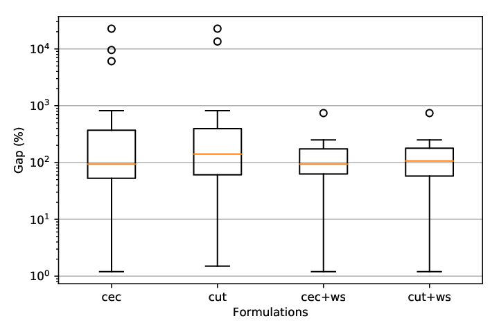
To summarize, the benchmark set considered in this section is composed of very challenging instances. The results indicate that even though nearly all original benchmark instances are solved, there is still room for advances in these approaches to solve these larger instances. Furthermore, the use of warm starts was shown to be a very important contribution when compared to the use of the plain formulations, as they became much more stable when it comes to the achieved optimality gaps. This is also depicted in Figure 6. It can be noticed that the improvements were more significant for formulation cut.
| Instance | cec | cut | G-HLIPP | cec + warm start | cut + warm start | ||||||||||
| Obj | UB | Gap (%) | Obj | UB | Gap (%) | Obj | Obj | UB | Gap (%) | Obj | UB | Gap (%) | |||
| 7-cube | 128 | 448 | 50 | 67 | 34.0 | 48 | 67 | 39.6 | 48 | 49 | 66 | 34.7 | 49 | 67 | 36.7 |
| 8-cube | 256 | 1,024 | 88 | 139 | 58.0 | 86 | 139 | 61.6 | 84 | 86 | 140 | 62.8 | 87 | 140 | 60.9 |
| 9-cube | 512 | 2,304 | 143 | 285 | 99.3 | 145 | 285 | 96.6 | 160 | 160 | 284 | 77.5 | 160 | 284 | 77.5 |
| Rand_200_796_10203 | 200 | 796 | 86 | 101 | 17.4 | 84 | 101 | 20.2 | 67 | 86 | 102 | 18.6 | 85 | 101 | 18.8 |
| Rand_200_3184_11203 | 200 | 3,184 | 32 | 62 | 93.8 | 33 | 62 | 87.9 | 30 | 30 | 62 | 106.7 | 30 | 62 | 106.7 |
| Rand_200_12139_12283 | 200 | 12,139 | 11 | 56 | 409.1 | 11 | 56 | 409.1 | 12 | 12 | 42 | 250.0 | 12 | 42 | 250.0 |
| Rand_300_1644_12739 | 300 | 1,644 | 101 | 149 | 47.5 | 93 | 149 | 60.2 | 82 | 92 | 150 | 63.0 | 97 | 150 | 54.6 |
| Rand_300_7026_13787 | 300 | 7,026 | 35 | 92 | 162.9 | 36 | 99 | 175.0 | 33 | 34 | 91 | 167.6 | 33 | 91 | 175.8 |
| Rand_300_27209_14811 | 300 | 27,209 | 11 | 101 | 818.2 | 11 | 101 | 818.2 | 12 | 12 | 101 | 741.7 | 12 | 101 | 741.7 |
| Toro_10_10_1187 | 100 | 200 | 59 | 61 | 3.4 | 59 | 62 | 5.1 | 54 | 59 | 61 | 3.4 | 59 | 62 | 5.1 |
| Toro_20_20_2283 | 400 | 800 | 259 | 262 | 1.2 | 259 | 263 | 1.5 | 213 | 259 | 262 | 1.2 | 259 | 262 | 1.2 |
| Toro_23_23_2595 | 529 | 1,058 | 344 | 349 | 1.5 | 344 | 349 | 1.5 | 282 | 344 | 349 | 1.5 | 344 | 349 | 1.5 |
| ba.1000.10.0 | 1,000 | 9,900 | 232 | 511 | 120.3 | 213 | 513 | 140.8 | 130 | 269 | 511 | 90.0 | 236 | 512 | 116.9 |
| ba.1000.10.1 | 1,000 | 9,900 | 271 | 513 | 89.3 | 278 | 513 | 84.5 | 135 | 272 | 512 | 88.2 | 271 | 513 | 89.3 |
| ba.1000.10.2 | 1,000 | 9,900 | 263 | 510 | 93.9 | 241 | 512 | 112.4 | 123 | 232 | 510 | 119.8 | 268 | 511 | 90.7 |
| ba.1000.10.3 | 1,000 | 9,900 | 304 | 511 | 68.1 | 208 | 515 | 147.6 | 128 | 264 | 512 | 93.9 | 284 | 514 | 81.0 |
| ba.1000.10.4 | 1,000 | 9,900 | 270 | 511 | 89.3 | 107 | 515 | 381.3 | 131 | 169 | 511 | 202.4 | 205 | 513 | 150.2 |
| ba.1000.3.0 | 1,485 | 13,860 | 7 | 675 | 9542.9 | 168 | 674 | 301.2 | 252 | 252 | 675 | 167.9 | 252 | 675 | 167.9 |
| ba.1000.3.1 | 1,485 | 13,860 | 11 | 679 | 6072.7 | 156 | 680 | 335.9 | 253 | 254 | 680 | 167.7 | 254 | 680 | 167.7 |
| ba.1000.3.2 | 1,485 | 13,860 | 158 | 679 | 329.7 | 134 | 681 | 408.2 | 234 | 234 | 680 | 190.6 | 234 | 680 | 190.6 |
| ba.1000.3.3 | 1,485 | 13,860 | 3 | 683 | 22666.7 | 3 | 684 | 22700.0 | 241 | 241 | 683 | 183.4 | 241 | 683 | 183.4 |
| ba.1000.3.4 | 1,485 | 13,860 | 105 | 680 | 547.6 | 84 | 684 | 714.3 | 243 | 243 | 682 | 180.7 | 243 | 682 | 180.7 |
| yeast | 2,361 | 6,646 | 226 | 516 | 128.3 | 4 | 543 | 13475.0 | 188 | 286 | 509 | 78.0 | 188 | 646 | 243.6 |
| Number of best values | 9 | 16 | 10 | 6 | 7 | 3 | 7 | 14 | 15 | 13 | 12 | 9 | 11 | ||
| Average gap (%) | 1804.1 | 1764.3 | 134.4 | 138.8 | |||||||||||
4 Concluding remarks
In this paper, we proposed two new formulations with an exponential number of constraints for the longest induced path problem on general graphs, together with effective branch-and-cut procedures for its solution. We proved that the polyhedra defined by formulation cut (wich ensures connectivity via cutset constraints) and by a state-of-the-art formulation, recently proposed in the literature Bökler et al. (2020), are equivalent. Besides, we showed that they are strictly contained in the polyhedron defined by formulation cec (which is based on constraints that explicitly eliminate cycles). We also analyzed the strength of clique inequalities when using variables corresponding to edges and to vertices.
Extensive computational experiments showed that our newly proposed approach based on the explicit elimination of cycles, although less strong in theory, performs very well in practice. More specifically, it outperforms the others as it is able to solve all but one of the 1065 benchmark instances used so far in the literature, showing a clear advantage especially for the more challenging instances.
In addition, we performed extended computational experiments on a newly proposed benchmark set consisting of 23 hard-to-solve larger instances, which poses a tough challenge to our approaches. These extended experiments also showed that offering initial feasible solutions to our formulations had a very positive impact in reducing the variability of the achieved optimality gaps.
Acknowledgments
Work of Ruslán G. Marzo was supported by a scholarship from Coordenação de Aperfeiçoamento de Pessoal de Nível Superior (CAPES) and by scholarship E-26/200.330/2020 from Fundação de Amparo à Pesquisa do Estado do Rio de Janeiro (FAPERJ). Work of Rafael A. Melo was supported by the State of Bahia Research Foundation (FAPESB) and the Brazilian National Council for Scientific and Technological Development (CNPq). Work of Celso C. Ribeiro was partially supported by CNPq research grants 303958/2015-4, 425778/2016-9, and and by FAPERJ research grant E-26/202.854/2017. This work was also partially sponsored by CAPES, under Finance Code 001.
References
- Agra et al. ((2017)) Agra, A., Dahl, G., Haufmann, T.A. & Pinheiro, S.J. (2017). The -regular induced subgraph problem. Discrete Applied Mathematics 222 14–30.
- Álvarez-Miranda et al. ((2013)) Álvarez-Miranda, E., Ljubić, I. & Mutzel, P. (2013). The maximum weight connected subgraph problem. In M. Jünger & G. Reinelt (Eds.), Facets of Combinatorial Optimization: Festschrift for Martin Grötschel ( 245–270). Berlin: Springer.
- Barabási & Albert ((1999)) Barabási, A-L. & Albert, R. (1999). Emergence of scaling in random networks. Science 286 5439 509–512.
- Bökler et al. ((2019)) Bökler, F., Chimani, M., Wagner, M.H. & Wiedera, T. (2019). Longest induced path. http://tcs.uos.de/research/lip online document, last access on April 4, 2021
- Bökler et al. ((2020)) Bökler, F., Chimani, M., Wagner, M.H. & Wiedera, T. (20201). An experimental study of ILP formulations for the longest induced path problem. In M. Baïou, B. Gendron, O. Günlük & A.R. Mahjoub (Eds.), Combinatorial Optimization ( 89–101). Cham: Springer International Publishing.
- Bökler et al. ((2020)) Bökler, F., Chimani, M., Wagner, M.H. & Wiedera, T. (20202). An experimental study of ILP formulations for the longest induced path problem. ArXiv arXiv:2002.07012 . https://arxiv.org/abs/2002.07012
- Bonomo et al. ((2018)) Bonomo, F., Chudnovsky, M., Maceli, P., Schaudt, O., Stein, M. & Zhong, M. (2018). Three-coloring and list three-coloring of graphs without induced paths on seven vertices. Combinatorica 38 779–801.
- Bron & Kerbosch ((1973)) Bron, C. & Kerbosch, J. (1973). Algorithm 457: Finding all cliques of an undirected graph. Communications of the ACM 16 575–577.
- Brunetta et al. ((2000)) Brunetta, L., Maffioli, F. & Trubian, M. (2000). Solving the feedback vertex set problem on undirected graphs. Discrete Applied Mathematics 101 37–51.
- Carrabs et al. ((2011)) Carrabs, F., Cerulli, R., Gentili, M. & Parlato, G. (2011). A Tabu Search Heuristic Based on k-Diamonds for the Weighted Feedback Vertex Set Problem. In J. Pahl, T. Reiners & S. Voß (Eds.), Network Optimization ( 6701, 589–602). Berlin: Springer.
- Chartrand et al. ((1993)) Chartrand, G., Johns, G.L. & Tian, S. (1993). Detour distance in graphs. Annals of Discrete Mathematics 55 127–136.
- Chudnovsky et al. ((2019)) Chudnovsky, M., Schaudt, O., Spirkl, S., Stein, M. & Zhong, M. (2019). Approximately coloring graphs without long induced paths. Algorithmica 81 3186–3199.
- Cormen et al. ((2009)) Cormen, T.H., Leiserson, C.E., Rivest, R.L. & Stein, C. (2009). Introduction to Algorithms (3rd ed.). : The MIT Press.
- Costa et al. ((2009)) Costa, A.M., Cordeau, J-F. & Laporte, G. (2009). Models and branch-and-cut algorithms for the Steiner tree problem with revenues, budget and hop constraints. Networks 53 141–159.
- Garey & Johnson ((1979)) Garey, M. & Johnson, D. (1979). Computers and intractability: A guide to the theory of NP-completeness. : WH Freeman and Company.
- Gavril ((2002)) Gavril, F. (2002). Algorithms for maximum weight induced paths. Information Processing Letters 81 203–208.
- Goemans & Myung ((1993)) Goemans, M.X. & Myung, Y-S. (1993). A catalog of steiner tree formulations. Networks 23 1 19–28.
- Golovach et al. ((2014)) Golovach, P.A., Paulusma, D. & Song, J. (2014). Coloring graphs without short cycles and long induced paths. Discrete Applied Mathematics 167 107–120.
- Hood et al. ((2015)) Hood, S., Recoskie, D., Sawada, J. & Wong, D. (2015). Snakes, coils, and single-track circuit codes with spread . Journal of Combinatorial Optimization 30 1 42–62.
- Ishizeki et al. ((2008)) Ishizeki, T., Otachi, Y. & Yamazaki, K. (2008). An improved algorithm for the longest induced path problem on -chordal graphs. Discrete Applied Mathematics 156 3057–3059.
- Jaffke et al. ((2020)) Jaffke, L., Kwon, O-j. & Telle, J.A. (2020). Mim-width I. Induced path problems. Discrete Applied Mathematics 278 153–168.
- Kaminski et al. ((2018)) Kaminski, J., Schober, M., Albaladejo, R., Zastupailo, O. & Hidalgo, C. (2018). Moviegalaxies - Social Networks in Movies. : Harvard Dataverse. https://doi.org/10.7910/DVN/T4HBA3 last access on April 5, 2021
- Kautz ((1958)) Kautz, W.H. (1958). Unit-distance error-checking codes. IRE Transactions on Electronic Computers 2 179–180.
- Kratsch et al. ((2003)) Kratsch, D., Müller, H. & Todinca, I. (2003). Feedback vertex set and longest induced path on AT-free graphs. In International Workshop on Graph-Theoretic Concepts in Computer Science ( 309–321).
- Ljubić et al. ((2006)) Ljubić, I., Weiskircher, R., Pferschy, U., Klau, G.W., Mutzel, P. & Fischetti, M. (2006). An algorithmic framework for the exact solution of the prize-collecting steiner tree problem. Mathematical Programming 105 427–449.
- Lozin & Rautenbach ((2003)) Lozin, V. & Rautenbach, D. (2003). Some results on graphs without long induced paths. Information Processing Letters 88 167–171.
- Lucena et al. ((2013)) Lucena, A., Salles da Cunha, A. & Simonetti, L. (2013). A new formulation and computational results for the simple cycle problem. Electronic Notes in Discrete Mathematics 44 83-88.
- Magnanti & Wolsey ((1995)) Magnanti, T.L. & Wolsey, L.A. (1995). Optimal trees. In Network Models ( 7, 503–615). : Elsevier.
- Marzo & Ribeiro ((2021)) Marzo, R.G. & Ribeiro, C.C. (2021). Exact and approximate algorithms for the longest induced path problem. RAIRO Operations Research 55 333–353.
- Matsypura et al. ((2019)) Matsypura, D., Veremyev, A., Prokopyev, O.A. & Pasiliao, E.L. (2019). On exact solution approaches for the longest induced path problem. European Journal of Operational Research 278 546–562.
- Melo et al. ((2021)) Melo, R.A., Queiroz, M. & Ribeiro, C.C. (2021). Compact formulations and an iterated local search-based matheuristic for the minimum weighted feedback vertex set problem. European Journal of Operational Research 289 75–92.
- Melo & Ribeiro ((2021)) Melo, R.A. & Ribeiro, C.C. (2021). Maximum weighted induced forests and trees: New formulations and a computational comparative review. ArXiv 2102.09194 . https://arxiv.org/abs/2102.09194
- Moon & Moser ((1965)) Moon, J.W. & Moser, L. (1965). On cliques in graphs. Israel Journal of Mathematics 3 23–28.
- Östergård & Pettersson ((2015)) Östergård, P.R. & Pettersson, V.H. (2015). Exhaustive search for snake-in-the-box codes. Graphs and Combinatorics 31 4 1019–1028.
- PassMark ((2021)) PassMark. (2021). PassMark Software - CPU Benchmarks. Intel Core i7-8700 vs Intel Xeon Gold 6134. https://www.cpubenchmark.net/compare/Intel-i7-8700-vs-Intel-Xeon-Gold-6134/3099vs3008 Last access on March 22, 2021
- Rehfeldt & Koch ((2019)) Rehfeldt, D. & Koch, T. (2019). Combining NP-hard reduction techniques and strong heuristics in an exact algorithm for the maximum-weight connected subgraph problem. SIAM Journal on Optimization 29 369–398.
- Tomita et al. ((2006)) Tomita, E., Tanaka, A. & Takahashi, H. (2006). The worst-case time complexity for generating all maximal cliques and computational experiments. Theoretical Computer Science 363 28–42.
- Yehezkeally & Schwartz ((2012)) Yehezkeally, Y. & Schwartz, M. (2012). Snake-in-the-box codes for rank modulation. IEEE Transactions on Information Theory 58 5471–5483.
Appendix A State-of-the-art integer programming formulation
The state-of-the-art integer programming formulation for the longest induced path problem was proposed by Bökler et al. (2020); Bökler et al. (2020). It considers the transformed graph , with and . Given the variables described in Section 2, their base formulation can be defined as
| (13) | |||||
| (14) | |||||
| (15) | |||||
| (16) | |||||
| (17) | |||||
The authors have observed that constraints (15) are equivalent to the generalized subtour elimination constraints (10). They also proposed a modified formulation using the variables (described in Section 2) and relaxes the integrality requirements on the variables. It can be cast as
| (18) | |||||
| (19) | |||||
| (20) | |||||
| (21) | |||||
We remark that Bökler et al. (2020); Bökler et al. (2020) tested several configurations of their formulation. We refer to as the best performing approach in their computational experiments, considering the number of instances solved to optimality and the average times for solving them. uses formulation BCWWy, add the clique inequalities (11) corresponding to all maximal cliques a priori to the formulation, and separates the cutset inequalities (15) only for integer solutions. Additionally, denotes the variant of without the addition of clique inequalities.
Appendix B Theoretical comparison of the formulations cec, cut and BCWWy
Denote by , , and the polyhedra defined by the linear relaxations of formulations cec, cut, and BCWWy, respectively. Each of these polyhedra is defined as the set of feasible points satisfying all the corresponding constraints. We remark that the objective functions (1) and (13) are equivalent, even for the linear relaxations of the formulations.
B.1 Comparing with
In what follows, we show that . Consider a solution . The proof consists in showing that and that there is a solution such that . Firstly, notice that the only difference between these two formulations is related to the constraints to remove cycles, namely, (4) for cec and (9) for cut.
Lemma 1.
Solution satisfies (4).
Proof.
First, remember that constraints (9) imply (10)Goemans & Myung (1993); Bökler et al. (2020). Consider any cycle . As (10) implies that for every , any right-hand side is at most . Thus, satisfies (4). ∎
Lemma 2.
.
Proof.
The proof follows from Lemma 1 together with the fact that all other constraints defining these polyhedra are the same. ∎
Lemma 3.
.
Proof.
Proposition 1.
.
B.2 Comparing with
In the following, we demonstrate that . Consider a solution . We show that . After that, we show that any solution also belongs to .
Proof.
Lemma 5.
Solution satisfies (15).
Lemma 6.
Solution satisfies (16).
Proof.
Assume without loss of generality that . Summing up inequalities (2) for and , we get
| (22) |
Firstly, we show that the inequality on the left is satisfied, namely, that
Observe that constraints (5) imply that . This, together with (22), ensures that
| (23) |
We now show that the inequality on the right is fulfilled, namely, that
Notice that whenever , the inequality is satisfied due to (22), since the right-hand side would sum up to at most two and the left hand side only has nonnegative terms. Now, assume that . Constraints (22) can be rewritten as
| (24) |
We now claim that the right-hand side of (24) is at most two. Observe that (6), together with the fact that we assumed that , implies that
| (25) |
Observe that could be substituted by its lower bound as it was ensured to be positive, given the assumptions.
As a consequence, satisfies (16). ∎
Lemma 7.
.
Now, consider . As Lemma 4 already discusses the equivalence of several of the constraints, it only remains to show that satisfies constraints (5) and (6).
Lemma 8.
Solution satisfies (5).
Proof.
Lemma 9.
Solution satisfies (6).
Proof.
Lemma 10.
.
Proposition 2.
.
Proposition 3.
.
Appendix C Comparing the strength of the different clique inequalities
We claim that the clique inequality on the edge variables (11) is as strong as the inequality on the vertex variables (12), under certain conditions.
Proof.
Proof.
Proposition 4.
Proof.
The proof consists in showing two examples of feasible fractional solutions belonging to . The first example, depicted in Figure 8, presents a solution that fulfills the inequality (12) but does not respect the inequality (11). The second one, illustrated in Figure 9, presents a solution that satisfies the inequality (11) but does not respect the inequality (12).
∎