∎

Embedding Reservoirs in Industrial Models to Exploit their FlexibilityThanks: This research was supported by the public service of Wallonia, within the framework of the InduStore project (grant 1450300).

Thibaut Cuvelier

Received: date / Accepted: date

Abstract

In the context of energy transition, industrial plants that heavily rely on electricity face more and more price volatility. To continue operating in these conditions, the directors become continually more willing to increase their flexibility, i.e. their ability to react to price fluctuations. This work proposes an intuitive methodology to mathematically model electro-intensive processes in order to assess their flexibility potential. To this end, we introduce the notion of reservoir, a storage of either material or energy, that allows models based on this paradigm to have interpretations close to the physics of the processes. The design of the reservoir methodology has three distinct goals: ( $i$ ) to be easy and quick to build by an energy-sector consultant; ( $ii$ ) to be effortlessly converted into mixed-integer linear or nonlinear programs; ( $iii$ ) to be straightforward to understand by nontechnical people, thanks to their graphic nature. We apply this methodology to two industrial case studies, namely an induction furnace (linear model) and an industrial cooling installation (nonlinear model), where we can achieve significant cost savings. In both cases, the models can be quickly written using our method and solved by appropriate solver technologies.

Keywords:

Electro-intensive industrial process Electricity-price volatility Mixed-integer linear programming Global optimisation

1 Introduction

Current industries tend to consume large quantities of energy, often electricity, during several stages of their processes: in aluminium production, to extract the material from alumina; in cement making, to crush the limestone and heat the kiln; in paper fabrication, to pulp the ground wood. An industrial site is said to be electro-intensive when the costs of energy compose a large part of the retail price. In this case, the dependency on electricity prices is very high in order to remain competitive. The literature mostly focuses on electricity in this context, as its price can be very volatile, as opposed to other fuels like natural gas.

Nevertheless, these industrial sites can often tune their processes in order to decrease their electricity consumption during the most expensive periods; they could also benefit from selling flexibility services to the electrical network, by reducing their consumption when the operator asks for it (Asadinejad and Tomsovic 2017). To achieve this cost reduction, they can make use of decision-support systems based on mathematical modelling of their processes. For example, the heating of a cement kiln can be reduced when the price is too high, or completely stopped if the revenue from the cement is not sufficient to cover the production costs. However, the achieved consumption drop is frequently the result of a trade-off:

•

in some cases, the system is operated differently to use another fuel (fuel switching), and this has little to no impact on the process. For instance, a cement kiln can switch from natural gas to flare gas or other industrial by-products (Bosoaga et al. 2009); in ethylene production, production plants can typically use several fuels including naphtha or Diesel oil (Petracci et al. 1996; Han et al. 2020);
•

in others, the only flexibility is to stop the process and lose some production (load shedding), which means that some orders cannot be fulfilled. For example, in aluminium smelting, any reduction of the current fed into the electrolysis potlines implies a loss of production (Todd et al. 2008);
•

other flexibility levers can be available, such as load shifting or scheduling, depending on the exact process, with varying degrees of impact on the production and the consumption. The paper industry falls in this category, with production plan reordering (Dejemeppe et al. 2016).

Indeed, the plant directors would welcome global models, describing the whole set of processes, that allow them to make the best decisions for their energy consumption based on price forecast. To this end, each industrial process in the factory should be modelled to provide a consumption-production mathematical formulation. These models do not need to offer highly detailed insights into the machines: the goal is not to have a real-time control of the physics thereof. In fact, our aim is rather to get an estimation of the consumption of the process depending on how it is operated. Moreover, the staff might not have the required knowledge of operational research to build such models: they have to rely on external consultants to do so.

This article proposes a generic paradigm to help conceiving such approximate formulations, so that they can be used to characterise the flexibility of a given process by the means of mathematical optimisation. The low-level basic block of this paradigm is the reservoir, which yields simple optimisation models while having a great expressive power.

For example, an oven might be modelled as two such reservoirs: a material tank (expressed in tonnes), and an energy storage (in joules). Over time, the oven loses some thermal energy, which can be modelled as losses from the energy reservoir. The oven is mainly controlled by its temperature, constrained to some operating range; this temperature is determined as a function of both the material and the energy reservoirs. The expressive power of the proposed paradigm comes from the fact that a reservoir may represent an actual physical storage or be more abstract (such as an energy storage or any quantity useful for modelling).

The complete oven model must also contain other blocks, named processes: these can impact the reservoirs, such as heating the oven. Only those processes might consume energy, such as electricity or natural gas for oven burners. A set of reservoirs only represents the state of the industrial machine, while processes interact with this state.

Using reservoir-based models for industrial processes has several advantages over typical ad-hoc models, especially in the context of building many such models in a short amount of time:

•

Reservoir-based models are built from a small number of intuitive components (described in Section 2). Consultants could quickly grasp the main ideas.
•

Reasoning about such a model is easier than with pure mathematical notations, as this paradigm suggests representing the processes as legible diagrams. This graphical representation helps communicate with technical experts of the industrial process and nontechnical managers.
•

The resulting optimisation models are often linear mixed-integer (MILPs).
•

Conversion into computer code is straightforward once the building blocks are implemented. A software implementation may even propose a graphical interface to build the complete optimisation model, similar to MATLAB Simulink (The MathWorks 2020). Almost no adaptations are then required to fit the parameters of such a model to known data (as highlighted in Section 6.1).

This article first details the developed reservoir taxonomy in Section 2, and some usage examples in Section 3, including diagrams. Even though the resulting problems are generally linear, more complex (i.e. nonlinear) behaviours can be implemented, as explained in Section 4. Based on this experience, we build a typology of processes in Section 5. Our numerical results are presented in Section 6, both for fitting a reservoir model to industrial data and for assessing the flexibility within an industrial site. We conclude in Section 7.

2 Reservoir taxonomy

To develop the aforementioned simplified models, four kinds of building blocks are needed. Each of them is directly associated to a mathematical formulation. In the following notations, boldface indicates optimisation variables, as opposed to constants, typeset in roman.

•

The reservoir, which is as close to the intuition of storage as possible: the level $\mathbf{s}_{t}$ is only impacted by the inflow $\mathbf{in}_{t}$ and the outflow $\mathbf{out}_{t}$ .

$\mathbf{s}_{t+1}=\mathbf{s}_{t}+\mathbf{in}_{t}-\mathbf{out}_{t}.$ (1)

These inflow and outflow variables link the reservoir to other parts of a global plant model. In the paper industry, for instance, the excess of pulp production may be stored before it is used by the paper machines, which indicates some decoupling between the production and the consumption — in other words, a source of flexibility.
•

The decaying reservoir, whose distinct feature is to have leaks $\mathbf{decay}_{t}$ in its content.

$\mathbf{s}_{t+1}=\mathbf{s}_{t}+\mathbf{in}_{t}-\mathbf{out}_{t}-\mathbf{decay}_{t}.$ (2)

Those leaks can be modelled with any kind of mathematical relationship: they can depend on the state of the reservoir $\mathbf{s}_{t}$ , but also on the state of other reservoirs. For example, an industrial oven naturally loses some thermal energy over time.
•

The observer, which is not a reservoir per se. Its state is a function of other reservoirs’ state, denoted by the variables $\mathbf{u}_{t},\mathbf{v}_{t}\dots$ :

$\mathbf{s}_{t}=f\!\left(\mathbf{u}_{t},\mathbf{v}_{t}\dots\right).$ (3)

It is mainly useful to implement bounds based on the state of a reservoir, such as the temperature in an oven, when it is modelled with both an energy and a mass reservoirs.
•

On top of these, external processes must be added to impact the state of the reservoirs, by imposing some value to the inflow and outflow variables. Two examples are heaters (they increase the level of a given heat reservoir) and chemical reactions (they transform some products into some others).

Each of these reservoirs may impose constraints on its level variable $\mathbf{s}_{t}$ , such as bounds (like minimum and maximum temperatures), ramping constraints (e.g., to limit the temperature variations), or process-dependent constraints (an oven cannot be tapped before its content is melted, for instance).

The flows between reservoirs may need to be coupled, especially when a given process is modelled as multiple reservoirs. This kind of constraint is common for heat transfer, for example: the quantity of heat transferred is proportional to the flow of heat-transfer fluid.

Aggregating those building blocks constructs models for the whole process. The final step to mathematically formulate the complete plant is to assemble the various systems in one model.

3 Reservoir models

This section shows a series of models that can be obtained with the methodology described in Section 2. All the examples are taken from the industry, with HVAC (Section 3.1) being present in many sites; ovens (Section 3.2) are mostly present in metallurgy, whereas electrolysis (Section 3.3) is a major process in chemistry. These examples are all electro-intensive processes: a typical metallurgical EAF is around 30 MW, while it is not uncommon to have electrolysis potlines of 50 MW.

Our goal is to produce simple and approximate models: they are used to detect the flexibility potential of a plant, not to perform complex real-time control on the processes. This is why linear models are usually good enough for our purposes. Would they fail in giving a good enough estimation, nonlinearities would have to be introduced (as done in Section 4).

One of the main advantages of the proposed methodology is that the models can be summarised by drawings, while retaining many details. This allows easy designing of models, while the actual formulation for the links between the reservoirs must be dealt with in more details outside the drawings.

3.1 HVAC

Heating, ventilation, and air conditioning (HVAC) is a kind of system often found in the industry (food processing, supermarket warehouses, pharmaceutical plants, etc.), but also in offices. This kind of process is usually not the most electro-intensive that can be found, but the industrial partners often agree with its flexibilisation (as opposed to their main business).

The proposed model works on a single energy reservoir, corresponding to the room whose temperature is controlled (or a set of rooms, or an industrial shed), as shown in Figure 1. Exploiting the thermal inertia of the area, the HVAC system can be turned off to save on energy while keeping an acceptable temperature.

Refer to caption — Figure 1: An HVAC installation modelled with reservoirs.

A series of external processes heats or cools down the room by adding or removing energy (heating and air conditioning): they are the inputs and outputs of the reservoir. Moreover, the reservoir level decreases due to thermal losses, which depend on the temperature difference between the inside and the outside. An observer reservoir is used to control directly the room temperature.

The corresponding mathematical formulation is the following.

•

The standard decaying reservoir model is used for the energy. It defines the main decision variable of this system: the energy within the room, denoted by $\mathbf{E}_{t}$ at time $t$ . Its state equation takes into account the heater ( $\mathbf{heating}_{t}$ ), the chiller ( $\mathbf{ac}_{t}$ ), and thermal losses ( $\mathbf{losses}_{t}$ ; these may very well be positive, if the outside temperature is higher than that of the room).

$\mathbf{E}_{t+1}=\mathbf{E}_{t}+\mathbf{heating}_{t}-\mathbf{ac}_{t}-\mathbf{losses}_{t}.$ (4)

The decay quantity $\mathbf{losses}_{t}$ can be approximated as directly proportional to the temperature difference between the room (denoted by $\mathbf{T}_{t}$ ) and the outside ( $T_{t}^{\mathrm{out}}$ ) (Crombie 2006), the coefficient being denoted by $k$ .

$\mathbf{losses}_{t}=k\times\left(\mathbf{T}_{t}-T_{t}^{\mathrm{out}}\right).$ (5)
•

Using an observer, the temperature is linked with the energy through the specific heat of the air $C_{p}$ and the mass of air in the room $m$ (which is considered constant):

$\mathbf{E}_{t}=C_{p}\times m\times\mathbf{T}_{t}.$ (6)

This temperature has strict bounds ( $T_{\min}$ and $T_{\max}$ ) that are imposed inside the observer:

$T_{\min}\leq\mathbf{T}_{t}\leq T_{\max}.$ (7)

Remark 1

As the mass of air $m$ is considered fixed, those constraints are linear. This approximation works well, because the volume of air to heat or cool down sees almost no variations in typical HVAC conditions. Section 3.1.1 considers a use case where this hypothesis no more holds.

•

External processes relate the heater and the chiller to their energy consumption (for example, electricity, $\mathbf{electricity}_{t}$ , and natural gas, $\mathbf{gas}_{t}$ ; a superscript $h$ denotes the chiller, while $ac$ is used for the air conditioning). The exact relationships $f$ and $g$ are not made explicit here:

\mathbf{heating}_{t}=f\!\left(\mathbf{electricity}_{t}^{\mathrm{h}},\mathbf{gas}_{t}^{\mathrm{h}}\right),

(8)

\mathbf{ac}_{t}=g\!\left(\mathbf{electricity}_{t}^{\mathrm{ac}},\mathbf{gas}_{t}^{\mathrm{ac}}\right).

(9)

These relationships may be either exact or approximated, depending on the need for precision. A basic model for these relations could use an efficiency or a coefficient of performance to relate the energy consumption and the produced effect (either heating or air conditioning).

•

The initial conditions indicate the state of the room to model at the beginning of the optimisation horizon, which gives the initial energy ( $\mathbf{E}_{0}$ ) based on the initial temperature ( $T_{0}$ ):

$\mathbf{E}_{0}=C_{p}\times m\times T_{0}.$ (10)

In a practical application, to fit this kind of model on experimental data, three important variables stand out: the energy that is pushed into or extracted from the room, the measured temperature, and the outside temperature. This data is sufficient to get the values for all the needed parameters ( $k$ for the losses and the product $C_{p}\,m$ for the temperature). With linear regressions, the parameter $C_{p}\,m$ is determined as the proportion coefficient between the energy and the temperature variations. With the same technique, the loss coefficient $k$ may be determined from (4).

This model is simpler than existing ones in the literature (Kusiak et al. 2010; Lee et al. 2015), but similar to models used in the context of flexibility (Short et al. 2019).

Remark 2

This formulation neglects the effects rooms may have on each other. Those may be included in such a model by using an energy reservoir per room. The losses would then depend on the connected rooms.
Also, the average specific heat variations in the room are neglected, as well as the temperature uniformity, i.e. the air is considered homogeneous.

3.1.1 Industrial cooling

A very similar model can be built for industrial cooling. The main differences are that no heating is performed, and that cooling can be done with two processes: either a cooling tower (whose efficiency depends on the outside temperature) or a chiller.

This model is more complicated due to the heat exchanges between the three components (the processes to cool and the two cooling mechanisms): the mass of heat- transfer fluid cannot be assumed to be constant. Indeed, the flows of hot and cooled water can be variable, but also the split between the two cooling processes. Each part of the model has two reservoirs: one for heat and the other for water, as shown in Figure 2. The flows between those reservoirs must be coupled by the means of temperature and the water’s heat capacity $C$ :

\mathbf{flow}_{\mathrm{heat}}=C\times\mathbf{T}\times\mathbf{flow}_{\mathrm{water}}.

(11)

The model is thus the following. Subscript $CT$ denotes the cooling tower, $p$ the processes that must be cooled, and $B$ the buffer to which the chiller is connected. The arrow $\to$ denotes a flow between two components.

•

Neither the water nor the heat reservoirs are decaying, as this decay is usually very small in these applications.

\mathbf{water_{CT,t+1}}=\mathbf{water_{CT,t}}+\mathbf{water_{p\to CT,t}}-\mathbf{water_{CT\to B,t}}.

(12)

\mathbf{water_{B,t+1}}=\mathbf{water_{B,t}}+\mathbf{water_{p\to B,t}}-\mathbf{water_{CT\to B,t}}.

(13)

	$\displaystyle\mathbf{E}_{CT,t+1}$	$\displaystyle=\mathbf{E}_{\mathrm{CT},t}+C_{\mathrm{water}}\times T_{p,t}\times\mathbf{water_{p\to CT,t}}$
		$\displaystyle-\mathbf{E}_{\mathrm{CT\to B},t}-f\!\left(\mathbf{P}_{\mathrm{CT},t}\right).$		(14)

	$\displaystyle\mathbf{E}_{B,t+1}$	$\displaystyle=\mathbf{E}_{B,t}+C_{\mathrm{water}}\times T_{\mathrm{p},t}\times\mathbf{water_{p\to B,t}}+\mathbf{E}_{\mathrm{CT\to B},t}$
		$\displaystyle-C_{\mathrm{water}}\times\mathbf{T}_{\mathrm{B},t}\times\mathbf{water_{B\to p,t}}-g\!\left(\mathbf{P}_{\mathrm{chiller},t}\right).$		(15)

•

The total water and energy from the processes must correspond to the input scenario.

$\mathbf{water_{p\to CT,t}}+\mathbf{water_{p\to B,t}}=\mathrm{water}_{\mathrm{p},t}.$ (16)
•

The flows of water and energy are linked.

$\mathbf{E}_{\mathrm{CT},t}=C_{\mathrm{water}}\times\mathbf{water_{CT,t}}\times\mathbf{T}_{\mathrm{CT},t}.$ (17)

$\mathbf{E}_{\mathrm{B},t}=C_{\mathrm{water}}\times\mathbf{water_{B,t}}\times\mathbf{T}_{\mathrm{B},t}.$ (18)

$\mathbf{E}_{\mathrm{CT\to B},t}=C_{\mathrm{water}}\times\mathbf{water_{CT\to B,t}}\times\mathbf{T}_{\mathrm{CT},t}.$ (19)
•

The buffer’s temperature must be within acceptable bounds for the processes, as its water is directly sent back to the processes.

$T_{\min}\leq\mathbf{T}_{\mathrm{B},t}\leq T_{\max}.$ (20)

This model is simpler than existing ones (Söderman and Ahtila 2010), even for similar applications, and has fewer parameters to fit (Peesel et al. 2019). Actually, in Section 6.2, we only use manufacturer-provided data to perform flexibility estimation. The real performance may significantly differ from the specifications (Peesel et al. 2017), but such a precision in the numerical results is usually not required for our use case.

A highly similar model can be used for petrochemical chains, like ethylene production (Han et al. 2020). More complex models can still be suited to mixed-integer linear formulations, but cannot be expressed as reservoirs; they also come with higher computational costs with traditional optimisation tools (Geng et al. 2020).

3.2 Oven

A more complex example of reservoir modelling is the industrial oven (see Figure 3), which heats large quantities of material (several tonnes) to high temperatures (around 1000 °C), usually with a high thermal inertia (which allows for turning off or reducing the heating from time to time). Different kinds of mechanisms can be used to heat the materials: gas or oil burners (for relatively low temperatures), electric arcs (for conductive materials), etc.

An oven model is similar to HVAC in that it has an energy reservoir. However, the main difference is that the quantity of material to heat may vary significantly, and thus cannot be neglected. This material is modelled as a second reservoir, coupled with the first one.

The relationships in this model are more intricate than in the previous ones: quantity of material, energy, and temperature are tightly and nonlinearly intertwined. For instance, when heating, the impact on temperature is not direct: for the same quantity of heating, the impact on temperature is less when the oven contains a large quantity of material than when it is almost empty.

In order for the oven to meet its operational goals, it must provide the needed quantities of material at the right temperature. When material is removed from the oven, it has lost an associated quantity of energy — but not temperature. However, when new material is inserted into the oven, this matter is at the outside temperature; it brings some energy into the oven, but lowers the overall temperature.

All in all, the obtained mathematical formulation is the following.

•

A first reservoir considers the material, $\mathbf{m}_{t}$ : some may be added ( $\Delta\mathbf{m}_{t}^{+}$ ) or removed ( $\Delta\mathbf{m}_{t}^{-}$ ) at any time step.

$\mathbf{m}_{t+1}=\mathbf{m}_{t}+\Delta\mathbf{m}_{t}^{+}-\Delta\mathbf{m}_{t}^{-}.$ (21)

•

A decaying reservoir is used for the energy. Adding or removing material has an impact on the energy content (with the specific heat $C_{p}$ , as previously). The withdrawn matter is at the oven temperature; however, the added material has a lower temperature, namely $T_{t}^{\mathrm{out}}$ :

\mathbf{E}_{0}=0,

(22)

$\displaystyle\mathbf{E}_{t+1}$	$\displaystyle=$	$\displaystyle\mathbf{E}_{t}+\mathbf{heating}_{t}-\mathbf{losses}_{t}$	(23)
	$\displaystyle+$	$\displaystyle C_{p}\times\Delta\mathbf{m}_{t}^{+}\times T_{t}^{\mathrm{out}}$
	$\displaystyle-$	$\displaystyle C_{p}\times\Delta\mathbf{m}_{t}^{-}\times\mathbf{T}_{t}$

The losses take the same form as previously, being linked to the temperature difference with the exterior:

\mathbf{losses}_{t}=k\times\left(\mathbf{T}_{t}-T_{t}^{\mathrm{out}}\right).

(24)

•

Likewise, an observer gives the temperature, but this time nonlinearly:

$\mathbf{E}_{t}=C_{p}\times\mathbf{m}_{t}\times\mathbf{T}_{t}.$ (25)

This nonlinearity is not a problem for the temperature bounds, as the constraint (7) can be rewritten in joules-kilograms without using constraint 25:

$C_{p}\times T_{\min}\times\mathbf{m}_{t}\leq\mathbf{E}_{t}\leq C_{p}\times T_{\max}\times\mathbf{m}_{t},$ (26)
•

The heater is still an external process that consumes energy:

$\mathbf{heating}_{t}=f\!\left(\mathbf{electricity}_{t},\mathbf{gas}_{t}\right).$ (27)

As opposed to the HVAC model, this formulation cannot be linear due to the losses, as they involve the temperature (24), i.e. the ratio between the energy and the mass. These issues are discussed in Section 4.

Remark 3

This model exploits the hypothesis that the specific heat $C_{p}$ remains constant with temperature. Also, it does not consider phase change, i.e. it only allows for heating material, not to melt it. A large quantity of energy being required for the material to change phase, adding this possibility in the model would require another reservoir that specifically deals with the molten part.

3.2.1 Induction furnace

Induction furnaces are a kind of industrial oven. They work by magnetic induction: the bucket containing the metal to melt (such as cast iron) is surrounded by a a coil through which high-voltage alternative currents are sent. The created magnetic field induces eddy currents in the metal, which in turn heats it. The power dissipated in the metal is directly proportional to the electrical power fed into the circuit $\mathbf{P}_{t}^{\mathrm{elec}}$ , with a constant ratio $\alpha$ , as shown in Section 8.

A reservoir model that fits this kind of furnace would be made up of two reservoirs: a mass reservoir that evolves at discrete time steps, and an energy decaying reservoir (filled and emptied at the same time as the mass reservoir). There is no need for a temperature observer, but only a “binary” observer that indicates whether the required total energy has been transferred to the metal at the end of the batch. The model is shown in Figure 4.

The corresponding model in mathematical form is the following:

•

The mass reservoir is fixed for a given batch:

$\mathbf{m}_{t}=m_{0}.$ (28)
•

The energy reservoir is filled by electrical currents:

$\mathbf{E}_{t+1}=\mathbf{E}_{t}+\alpha\,\mathbf{P}_{t}^{\mathrm{elec}}.$ (29)
•

The observer reservoir imposes that, at the end of the batch, the total energy in the bucket is at least at the required level:

$\mathbf{E}_{T}\geq f\!\left(m_{0}\right).$ (30)
•

Initially, the energy reservoir indicates that the material is at the exterior temperature:

$\mathbf{E}_{0}=C_{p}\times m_{0}\times T_{0}^{\mathrm{out}}.$ (31)

Typical models for such furnaces deal with the details of the electromagnetic field required to melt the metal (Abubakre et al. 2009; Naar and Bay 2013), which is too cumbersome for our application.

3.3 Electrolysis

The chemical industry and metallurgy often use electrolysis, with aluminium smelting being a prime example. A potline is typically made of hundreds of individual baths, where the electrochemical reactions take place. Each of them can be controlled independently and turned off to save energy, but with a loss of production (Todd et al. 2008).

In front of the potline, there is a single transformer from AC to DC current; its output has a relatively low voltage (around 5 V, usually), but very high amperage (multiple hundreds of kiloamperes are not rare) (Todd et al. 2008; Alcoa Inc. 2004; BALCO 2013). After the transformer, all pots resemble ovens (as in Section 3.2): they are heated by the current that flows through them, so that their bath remains in a given temperature range where the electrochemical reaction can happen.

The main difference with ovens is that the contents of the pots have smaller fluctuations: inputs are continuous, so the mass increases at a predictable and constant rate; the product is siphoned off periodically, typically once per day (Todd et al. 2008; Alcoa Inc. 2004; BALCO 2013). However, the contents of the bath continuously evolve: the alumina and the carbon anode are transformed into aluminium and gas, the actual reactions being $\text{Al}_{2}\text{O}_{3}{}+{}{}{}{}{}\mathrm{3}\,\mathrm{C}\,\to\,\mathrm{}{\vphantom{\mathrm{X}}}_{\smash[t]{\mathrm{2}}}\,\mathrm{Al}{}+{}{}{}\mathrm{3}\,\mathrm{CO}$ and $\text{2 }\text{Al}_{2}\text{O}_{3}{}+{}{}{}{}{}\mathrm{3}\,\mathrm{C}\,\to\,\mathrm{}{\vphantom{\mathrm{X}}}_{\smash[t]{\mathrm{4}}}\,\mathrm{Al}{}+{}{}{}\mathrm{3}\,\mathrm{CO}_{2}$ . As such, $415\,\mathrm{kg}$ of carbon anode (not fed continuously, the anode being replaced after a few weeks) are consumed to produce $1\,\mathrm{t}$ of metallic aluminium, and this carbon is ejected as exhaust gas (carbon mono- and dioxide) (The New Zealand Institute of Chemistry 2008). Nevertheless, these exhausts are neglected in our model.

The flexibility impacts the production in a slightly more complicated way than in the aforementioned processes: it depends (approximately linearly) on the average current through the pot, as long as the temperature is in the right range (which is controlled by voltage) (Molina-Garcia et al. 2011).

As a consequence, the electrolytic bath model contains four reservoirs:

The energy is included as a decaying reservoir, exactly like in the previous models (4) and (23), with some contribution due to the alumina input $\Delta\mathbf{m_{Al_{2}O_{3}}}_{t}^{+}$ and to the metallic aluminium output $\Delta\mathbf{m_{Al}}_{t}^{-}$ , but also to the fact that the reaction is exothermic (with $\Delta H$ being the enthalpy change due to the reaction):

$\displaystyle\mathbf{E}_{t+1}$	$\displaystyle=\mathbf{E}_{t}+\mathbf{heating}_{t}-\mathbf{losses}_{t}$	(32)
	$\displaystyle+C_{p}^{\mathrm{Al_{2}O_{3}}}\times\Delta\mathbf{m_{Al_{2}O_{3}}}_{t}^{+}\times T_{t}^{\mathrm{out}}$
	$\displaystyle-C_{p}^{\mathrm{Al}}\times\Delta\mathbf{m_{Al}}_{t}^{-}\times\mathbf{T}_{t}$
	$\displaystyle+\Delta H\times\Delta\mathbf{m_{Al}}_{t}^{+}\times\left(\mathbf{T}_{t}-T_{t}^{\mathrm{out}}\right)$	(33)

Again, the coefficient $C_{p}^{X}$ is the specific heat of material $X$ . The thermal losses can be expressed as linear with respect to the temperature difference with the outside:

\mathbf{losses}_{t}=k\times\left(\mathbf{T}_{t}-T_{t}^{\mathrm{out}}\right).

(34)

2.

The carbon anode reservoir can only be consumed by the electrochemical reaction (it is replaced during maintenance, which we do not mean to optimise):

$\mathbf{m_{C}}_{t+1}=\mathbf{m_{C}}_{t}-\Delta\mathbf{m_{C}}_{t}^{-}.$ (35)

The alumina reservoir is constantly fed, and consumed by the electrochemical reaction:

\mathbf{m_{Al_{2}O_{3}}}_{t+1}=\mathbf{m_{Al_{2}O_{3}}}_{t}+\Delta\mathbf{m_{Al_{2}O_{3}}}_{t}^{+}-\Delta\mathbf{m_{Al_{2}O_{3}}}_{t}^{-}.

(36)

4.

The aluminium reservoir is filled by the electrochemical reaction and periodically emptied:

$\mathbf{m_{Al}}_{t+1}=\mathbf{m_{Al}}_{t}+\Delta\mathbf{m_{Al}}_{t}^{+}-\Delta\mathbf{m_{Al}}_{t}^{-}.$ (37)

The temperature observer depends on the complete mass within the electrolytic bath. A simplifying assumption is to consider that the temperature is uniform within the bath:

\mathbf{E}_{t}=\left(C_{p}^{\mathrm{Al_{2}O_{3}}}\times\mathbf{m_{Al_{2}O_{3}}}_{t}+C_{p}^{\mathrm{C}}\times\mathbf{m_{C}}_{t}+C_{p}^{\mathrm{Al}}\times\mathbf{m_{Al}}_{t}\right)\,\mathbf{T}_{t}.

(38)

As for an oven (26), the temperature bounds can be written linearly based on this expression:

T_{\min}\times\left(C_{p}^{\mathrm{Al_{2}O_{3}}}\times\mathbf{m_{Al_{2}O_{3}}}_{t}+C_{p}^{\mathrm{C}}\times\mathbf{m_{C}}_{t}+C_{p}^{\mathrm{Al}}\times\mathbf{m_{Al}}_{t}\right)\leq\mathbf{E}_{t},

(39)

\mathbf{E}_{t}\leq T_{\max}\times\left(C_{p}^{\mathrm{Al_{2}O_{3}}}\times\mathbf{m_{Al_{2}O_{3}}}_{t}+C_{p}^{\mathrm{C}}\times\mathbf{m_{C}}_{t}+C_{p}^{\mathrm{Al}}\times\mathbf{m_{Al}}_{t}\right).

(40)

The last block within the process, the electrochemical reactions, are modelled as processes, whose conversion rates $k_{X}^{\prime\prime}$ depend on the average current through the bath ( $\mathbf{\overline{I}}_{t}$ ):

\Delta\mathbf{m_{Al}}_{t}^{+}=k_{{}\mathrm{Al}}^{\prime\prime}\times\mathbf{\overline{I}}_{t},\qquad\Delta\mathbf{m_{C}}_{t}^{-}=k_{{}\mathrm{C}}^{\prime\prime}\times\mathbf{\overline{I}}_{t},

(41)

\Delta\mathbf{m_{Al_{2}O_{3}}}_{t}^{-}=k_{{}\mathrm{Al}_{2}\text{O}_{3}}^{\prime\prime}\times\mathbf{\overline{I}}_{t}.

(42)

7.

The AC-DC converter must be modelled as an external process to provide the required power to heat the bath; moreover, the actual amperage must be explicitly represented in the model for the electrochemical reaction rate:

$\mathbf{heating}_{t}=f\!\left(\mathbf{electricity}_{t},\mathbf{\overline{I}}_{t}\right).$ (43)
8.

Finally, the initial conditions are set according to the way the process is managed: the process is rarely started from scratch (with a temperature equal to $T_{0}^{\mathrm{out}}$ ), but rather continuously operated.

The model is shown in Figure 5. Existing models tend to use electrochemical multiphysics techniques (Hofer 2011; Zhao et al. 2020), which are not well-suited for light applications like flexibility estimation.

Remark 4

The observer equation 38 might consider directly the sum of all three material reservoirs (alumina, carbon, and metallic aluminium), without a distinction between the various materials: their specific heats are of the same order of magnitude (between $700$ and $900\,\mathrm{J/K\,kg}$ ). This approximation is justified in the context of flexibility, as the model does not need to be very precise. This simplification is useful when fitting the model to actual data, as fewer parameters must be estimated.

Remark 5

If the electrical current is not considered for flexibilisation, then the model can be simplified, as the electrochemical reaction then becomes constant: the mass reservoir levels only change when the bath is powered on (and thus when the electrochemical reaction takes place). The only possible values are then naturally discrete.

4 Nonlinearity

Another great advantage of the proposed methodology is that most models are linear. However, these can be limiting for some behaviours that cannot be completely represented with linear equations. For those cases, such as ovens (for which a conceptual model is presented in Section 3.2), nonlinearities can be introduced in the reservoir formalism.

Those nonlinearities can be dealt with in different ways.

•

Use of nonlinear nonconvex solvers. Nonlinear equalities such as (38) make standard optimisation solvers unusable because of their nonconvexity. Therefore, the solvers must be able to deal with nonconvex constraints and (often) mixed-integer variables. Programs like Couenne (Belotti 2009), POD (Nagarajan et al. 2016) (global solvers, not relying on the convexity assumption), or Bonmin (Bonami and Lee 2013) (approximating the problem as convex) must then be used. The most recent versions of standard optimisation solvers like CPLEX (IBM 2020) and Gurobi (Gurobi Optimization LLC 2020) now allow for certain types of nonconvexity (CPLEX 12.7 accepts nonconvex quadratic objective functions, whereas Gurobi 9.0 also tackles quadratic nonconvex constraints).
•

Linear reformulations. Another option is to formulate the problem linearly. The main technique we used for this is discretisation: instead of having continuous variables, some of them are only allowed to take discrete levels. The choice of variables for discretisation is made so that, when these variables take a fixed value, the constraint becomes linear. For example, the constraint (38) is linear once the mass is known. Binary variables are then used to choose among the various discrete values, which keeps the overall linearity.

4.1 Discretisation

Discretisation is an approximation of the previous models. It can however be used in some cases without being a rough estimate, due to the actual operational conditions: for instance, industrial ovens are often loaded by batches, whose sizes can be used to define the discretisation levels.

An oven like in Section 3.2 can be reformulated with this discretisation approach, more specifically the temperature definition (25). Instead of having a continuous variable $\mathbf{m}_{t}$ , it takes its value in a discrete set $\mathcal{M}=\left\{\mathcal{M}_{i}\,|\,i\in\left[1,M\right]\right\}$ . For example, instead of having an oven whose mass may freely vary between $500\,\mathrm{kg}$ and $5\,\mathrm{t}$ , its discretised version may only take the values in $\mathcal{M}=\left\{500,1500,2500,3500,5000\right\}\,\mathrm{kg}$ , or $\mathcal{M}=\left\{500,1000,1500,2000,3500,5000\right\}\,\mathrm{kg}$ if more precision is needed for low masses.

In order to linearise the quotient $\mathbf{T}_{t}=\mathbf{E}_{t}/C_{p}\,\mathbf{m}_{t}$ , the following expression can be used:

	$\displaystyle\mathbf{T}_{t}$	$\displaystyle=\frac{\mathbf{E}_{t}}{C_{p}\,\mathbf{m}_{t}},\qquad\forall t\in\mathcal{T}$
		$\displaystyle=\begin{cases}\mathbf{E}_{t}/C_{p}\,\mathcal{M}_{1}&\mbox{ if }\mathbf{m}_{t}=\mathcal{M}_{1}\\ \mathbf{E}_{t}/C_{p}\,\mathcal{M}_{2}&\mbox{ if }\mathbf{m}_{t}=\mathcal{M}_{2}\\ \vdots\\ \mathbf{E}_{t}/C_{p}\,\mathcal{M}_{M}&\mbox{ if }\mathbf{m}_{t}=\mathcal{M}_{\text{$\left\|\mathcal{M}\right\|$}}\end{cases},\qquad\forall t\in\mathcal{T}.$

Implementing this in a mathematical optimisation model can be done in a classical way (Liberti 2009; Liberti and Maculan 2009; Vielma 2015). New variables are introduced:

•

The binary variables $\mathbf{m}_{t}^{\left(i\right)}$ indicates whether the material contents of the oven $\mathbf{m}_{t}$ take the discrete value $\mathcal{M}_{i}$ .
•

The continuous variable $\mathbf{T}_{t}$ is defined as the quotient $\mathbf{E}_{t}/C_{p}\,\mathbf{m}_{t}$ .
•

The continuous variable $\mathbf{T}_{t}^{\left(i\right)}$ is defined as the quotient $\mathbf{E}_{t}/C_{p}\,\mathbf{m}_{t}$ if $\mathbf{m}_{t}=\mathcal{M}_{i}$ , and zero otherwise. These variables could be called “partial temperatures”, as their sum yields the temperature.

Then, constraints are added to impose those semantics.

•

Exactly one discrete mass value is possible at any time step:

$\sum_{i\in\mathcal{M}}\mathbf{m}_{t}^{\left(i\right)}=1,\qquad\forall t\in\mathcal{T}.$ (44)
•

The mass is then defined as a linear combination of those binary choices:

$\mathbf{m}_{t}=\sum_{i\in\mathcal{M}}\mathbf{m}_{t}^{\left(i\right)}\,\mathcal{M}_{i},\qquad\forall t\in\mathcal{T}.$ (45)
•

Similarly, the temperature is given by the sum over all partial temperatures:

$\mathbf{T}_{t}=\sum_{i\in\mathcal{M}}\mathbf{T}_{t}^{\left(i\right)},\qquad\forall t\in\mathcal{T}.$ (46)

•

The partial temperatures $\mathbf{T}_{t}^{\left(i\right)}$ are linked to the binary choices by the following upper and lower bounds:

\mathbf{T}_{t}^{\left(i\right)}\geq\frac{\mathbf{E}_{t}}{C_{p}\,\mathcal{M}_{i}}-\frac{E_{\max}}{C_{p}\,m_{\mathrm{min}}}\,\left(1-\mathbf{m}_{t}^{\left(i\right)}\right),\qquad\forall t\in\mathcal{T},\quad\forall i\in\mathcal{M},

(47)

\mathbf{T}_{t}^{\left(i\right)}\leq\frac{\mathbf{E}_{t}}{C_{p}\,\mathcal{M}_{i}},\qquad\forall t\in\mathcal{T},\quad\forall i\in\mathcal{M},

(48)

\mathbf{T}_{t}^{\left(i\right)}\leq\frac{E_{\max}}{C_{p}\,m_{\min}}\,\mathbf{m}_{t}^{\left(i\right)},\qquad\forall t\in\mathcal{T},\quad\forall i\in\mathcal{M}.

(49)

The two last bounds are required to be specified separately, to ensure that a partial temperature is forced to be zero if the corresponding mass level is chosen, and takes its expected value otherwise.

Thanks to this technique, the temperature definition becomes linear. It could be extended to more general expressions.

This formulation can be strengthened in order to improve solving times. The bounds on the partial temperatures $\mathbf{T}_{t}^{\left(i\right)}$ should be as tight as possible to keep good solving times; this issue motivated the choice of temperature $\mathbf{T}_{t}=E_{t}/C_{p}\,\mathbf{m}_{t}$ over the raw quotient of variables $\mathbf{E}_{t}/\mathbf{m}_{t}$ , as the factor $1/C_{p}$ can reduce the values that are considered by several orders of magnitude.

•

The bounds on the partial temperatures also have lower bounds, using the same binary variables:

\mathbf{T}_{t}^{\left(i\right)}\geq\frac{E_{\mathrm{min}}}{C_{p}\,m_{\mathrm{max}}}\,\mathbf{m}_{t}^{\left(i\right)},\qquad\forall t\in\mathcal{T},\quad\forall i\in\mathcal{M}

(50)

•

The mutual exclusion of the $m_{t}^{\left(i\right)}$ can be further imposed with clique constraints:

\sum_{i\in\mathcal{V}}\mathbf{m}_{t}^{\left(i\right)}\leq 1,\qquad\forall t\in\mathcal{T},\quad\forall\mathcal{V}\subseteq\mathcal{M}:\>\left|\mathcal{V}\right|\geq 2

(51)

4.2 Benchmark

The two nonlinear models are benchmarked against each other, in order to compare their performance when solving the same problem. We use an oven-like model to heat a given quantity of metal that may be added at any rate and time (which gives a nonlinear model). Fifty time steps are considered. Heating happens with temperature ramping constraints. All models have been written using JuMP (Dunning et al. 2017) in Julia (Bezanson et al. 2017).

Those models are all compared to a base line, which heats the material as soon as possible (while respecting the same ramping constraints) and keeps it at the right temperature until the end of the horizon.

The results are shown in Table 1. When a high precision is needed in the discretised variables, both CPLEX (IBM 2020) and Gurobi (Gurobi Optimization LLC 2020), two state-of-the-art mixed-integer linear solvers, have troubles to reach a very low gap, albeit their solutions are more than satisfying for industrial applications. In the same time budget, the nonlinear formulation with open-source nonlinear solvers achieves a better solution, without being hindered by discretised variables.

Table 1: Solving time for the various nonlinear models. All solvers were stopped after approximately one hour of computations, even when they did not find the optimum solution (nonzero gap). Those tests were run on a machine with two Intel Xeon E5-2650v4 (2.2GHz) and 128GB of RAM.

Model	Underlying solver	Time (s)	Solution cost (€)	Gap reported by the solver (%)	Cost improvement with respect to reference (%)

Reference: reach target temperature as soon as possible	CPLEX 12.7.1	$0.02$	$10,793.25$	$0.00$	—
Reservoir model: linearisation by discretisation (16 levels)	CPLEX 12.7.1	$3,610.37$	$8,208.23$	$2.68$	$23.95$
	Gurobi 7.5.0	$3,600.02$	$8,034.72$	$2.12$	$25.56$



Reservoir model: nonlinear (continuous)	Bonmin 1.8.4	$3,600.59$	$7,259.46$	—	$32.74$
	Couenne 0.5.4	$3,601.39$	$7,260.20$	$100$	$32.73$

5 Process typology

Based on these models, we can derive a typology of industrial processes based on a few characteristics. Table 2 does so according to two criteria, focusing on the flows of material to process:

•

the inputs to the process: are they continuous or periodical?
•

the outputs from the process: are they continuous or periodical?

Those two questions can be equivalently formulated as follows. Is the mass currently processed constant? How can it vary (continuously, periodically)?

Combined, these three parameters indicate how the process could be modelled. A mass that is constant (HVAC) or highly predictable (electrolysis, batches; kilns to a lesser degree) can result in model simplifications. Completely variable masses often implies nonlinearity (as most ovens, see Section 4).

Table 2: Typology of industrial processes to help reservoir modelling.

Process	Mass	Inputs	Outputs

HVAC	Constant	(Constant mass: no inputs nor outputs)
Kiln	Variable	Continuous	Continuous
Oven (including electric arc furnace, induction furnace)	Batch	Discrete (batches: when starting)	Discrete (batches: when done, e.g. molten metal)
Electrolysis	Variable	Continuous	Discrete (periodical: e.g., every day)

The diagrams shown in Section 3 also help build another typology, this time based on the potential flexibility levers for each process. Indeed, the presence of a decaying heat energy reservoir indicates that the process is amenable to load shifting: even if heating is stopped, the process might still continue to produce, albeit probably at a lessened rate. If multiple fuels are possible for heating, then fuel switching can be used. For all non-continuous processes, load scheduling can be applied; for continuous processes whose production can be tuned (like electrolysis), exploiting flexibility may lead to load shedding. The processes that have been studied in Section 3 are included in Table 3.

Table 3: Analysis of flexibility levers available in industrial processes.

Process	Potential flexibility levers

HVAC	Thermal inertia: load shifting
Kiln	Thermal inertia: load shifting (production delayed)
Starting time: load scheduling
Fuel switching
Continuous oven	Thermal inertia: load shifting (production delayed)
Fuel switching
EAF	Thermal inertia: load shifting (production delayed)
Starting time: load scheduling
Electrolysis	Thermal inertia: load shifting
For a long period of time, becomes load shedding!

6 Flexibility potential of industrial processes

Some models developed in Section 3 are now fit to industrial data, and the flexibility potential of the processes is estimated based on historical scenarios. A major hypothesis is that exploiting the flexibility for these industrial sites has no impact on the electricity market, as they do not consume enough electricity.

All optimisation models have been written using JuMP (Dunning et al. 2017) in Julia (Bezanson et al. 2017). The source code for the simulations is available online at the following address:
https://github.com/dourouc05/IndustrialProcessFlexibilisation.jl

6.1 Induction furnace

The induction furnace of Section 3.2.1 needs three parameters. The first one, $\alpha$ , characterises the energy level depending on the initial temperature of the material. The second one, $\beta$ , is the efficiency of converting the electrical power into heat (see Appendix 8). The last one, $\delta$ , indicates the energy losses.

Each sample $s\in\mathcal{S}$ , taken from historical measurements, corresponds to one use of the furnace. It mainly consists in a power curve $P_{s}^{t}$ , indicating the average power injected through the circuits each hour (a melting cycle lasts twelve hours). To have a better fit, each sample may have its own value of $\beta$ , denoted by $\beta_{s}$ . The values of the $\beta_{s}$ are brought closer together by a constraint limiting the variance of the $\beta_{s}$ to $0.001$ . All in all, fitting the parameters is done through the following optimisation program (a convex QCQP), based on the reservoir model of Section 3.2.1:

\begin{array}[]{ccc}\min&\sum_{s\in\mathcal{S}}\left(\mathbf{E}_{s}^{t}-E_{s}\right)^{2}\\ \text{s.t.}&\mathbf{E}_{s}^{0}=\boldsymbol{\alpha}\times m_{s}\times T_{0}&\forall s\in\mathcal{S}\\ &\mathbf{E}_{s}^{t}=\mathbf{E}_{s}^{t-1}+\boldsymbol{\beta_{s}}\times P_{s}^{t}-\boldsymbol{\delta}&\forall s\in\mathcal{S},\forall t\in\mathcal{T}\\ &\left|\mathcal{S}\right|\times\boldsymbol{\overline{\beta}}=\sum_{s\in\mathcal{S}}\boldsymbol{\beta_{s}}\\ &\sum_{s\in\mathcal{S}}\left(\boldsymbol{\beta_{s}}-\mathbf{\boldsymbol{\overline{\beta}}}\right)^{2}\leq 0.001\\ &\boldsymbol{\alpha}\geq 0\\ &\boldsymbol{\beta}_{s}\geq 0&\forall s\in\mathcal{S}\\ &\mathbf{\boldsymbol{\overline{\beta}}}\geq 0\\ &\boldsymbol{\delta}\geq 0\end{array}

(52)

To evaluate the results of this model, we use a leave-one-out procedure (Efron 1982): for each sample $s\in\mathcal{S}$ , we solve the previous optimisation program over the samples $\mathcal{S}\backslash\left\{s\right\}$ to get a value $\beta_{\mathcal{S}\backslash\left\{s\right\}}$ , and we average the obtained square errors to predict the energy of $s$ based on $\beta_{\mathcal{S}\backslash\left\{s\right\}}$ . It results in a root mean square error on our data set of $65.194\,\text{kWh}$ (the ratio of this error to the average energy is $1.78\%$ ).

Once a reservoir model is fit, it can be used to estimate the flexibility potential of the process. To this end, we compare our reservoir-based optimisation to current fixed consumption profiles on a historical price scenario (an average day of January 2016 on the Belgian day-ahead market). No optimisation is currently performed on the schedule: the smelting process always starts at the same hour and lasts for twelve hours.

Related constraints must be added to the formulation in order to implement real-world constraints. Mostly, the peak power is limited, and the heating cannot abruptly change. Three constraints are thus added for each time step: a minimum and a maximum power ( $P_{\min}$ and $P_{\max}$ , respectively), and a ramping constraint ( $\rho_{\min}$ and $\rho_{\max}$ are respectively the minimum and maximum ratios by which the electrical consumption is allowed to change from hour to hour).

The complete model is therefore the following, where $p_{h}$ indicates the price of electricity for the hour $h$ (in €/MWh), $c_{h}$ the electrical consumption (in MWh), and $E_{h}$ the energy of the metal to melt:

\begin{array}[]{ccc}\min&\sum_{h=1}^{H}p_{h}\,c_{h}\\ \text{s.t.}&E_{0}=\alpha\,m\,T_{0},\\ &E_{H}=\alpha\,m\,T_{H},\\ &E_{h}=E_{h-1}+\beta\,c_{h}-\delta&\forall h\in\left\{1,2\dots H-1\right\}\\ &P_{\min}\leq c_{h}\leq P_{\max}&\forall h\in\left\{1,2\dots H\right\}\\ &\rho_{\min}\,c_{h}\leq c_{h+1}\leq\rho_{\max}\,c_{h}&\forall h\in\left\{1,2\dots H\right\}\end{array}

(53)

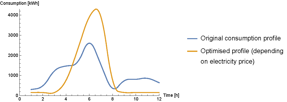
Per heat, using a reservoir model to decide the heating power, hour per hour, could decrease the costs by 8.35% per heat, from €239.11 to €219.15; over a year, this corresponds to more than €15,000 of savings. The main difference in the planned power consumption is that its peak is shifted to exploit the lowest prices during the production period (as shown in Figure 6).

Computationally speaking, this model allows to optimise the required power to a given price scenario in a fraction of a second: a 95% confidence interval is $0.03\pm 0.01$ seconds (with either CPLEX 12.7.1 or Gurobi 7.5.0). Fitting the parameters is also very quick, as the leave-one-out validation phase takes less than two minutes for the available data. The from-scratch implementation in Julia takes 150 lines, but the process could be automatised with a GUI to build the reservoir model. These characteristics are very appealing for energy-sector consultants, who may want to estimate the flexibility potential of an industrial site in very little time: most of the effort can be spent on actual discussions on the flexibility solutions that can be implemented.

6.2 Industrial cooling

Based on industrial data from a polypropylene-film plant, a model similar to that of Section 3.1.1 can be tuned. All the needed physical constants are known and match the data set. The model is then fed with scenarios of water volumes to cool down. In practice, the price scenarios can be estimated in advance, while the heat and water volumes are known with a high precision.

The processes in Figure 2 have to be specified in more details. A linear model is deemed sufficient for our needs, using coefficients of performance, and the functions $f$ and $g$ can be written as:

f\!\left(\mathbf{P}_{\mathrm{CT},t}\right)=\mathrm{cop}_{\mathrm{CT}}\times\mathbf{P}_{\mathrm{CT},t},

(54)

f\!\left(\mathbf{P}_{\mathrm{chiller},t}\right)=\mathrm{cop}_{\mathrm{chiller}}\times\mathbf{P}_{\mathrm{chiller},t}.

(55)

Thus, the two energy budget constraints (14) and (15) become:

	$\displaystyle\mathbf{E}_{\mathrm{CT},t+1}$	$\displaystyle=\mathbf{E}_{\mathrm{CT},t}+C_{\mathrm{water}}\times T_{\mathrm{p},t}\times\mathbf{water_{p\to CT,t}}$
		$\displaystyle-\mathbf{E}_{\mathrm{CT\to B},t}-\mathrm{cop}_{\mathrm{CT}}\times\mathbf{P}_{\mathrm{CT},t}.$

	$\displaystyle\mathbf{E}_{B,t+1}$	$\displaystyle=\mathbf{E}_{B,t}+C_{\mathrm{water}}\times T_{\mathrm{p},t}\times\mathbf{water_{p\to B,t}}+\mathbf{E}_{\mathrm{CT\to B},t}$
		$\displaystyle-C_{\mathrm{water}}\times\mathbf{T}_{\mathrm{B},t}\times\mathbf{water_{B\to p,t}}-\mathrm{cop}_{\mathrm{chiller}}\times\mathbf{P}_{\mathrm{chiller},t}.$

Two other constraints must be added for the cooling processes, as they have a limited maximum power:

\mathbf{P}_{\mathrm{CT},t}\leq P_{\mathrm{CT},\max},

(56)

\mathbf{P}_{\mathrm{chiller},t}\leq P_{\mathrm{chiller},\max}.

(57)

Remark 6

Variable coefficients of performance are not considered in this case in order to keep the model simple. The increased complexity is not justified in a context of approximate models.

In order to compare the impact of flexibility on the cooling behaviour, the temperature bounds are set in two different ways:

•

either $T_{\mathrm{target}}\pm 0.5\text{\textdegree C}$ (low-flexibility scenario), as currently implemented in the studied use case
•

or $T_{\mathrm{target}}\pm 3\text{\textdegree C}$ (high-flexibility scenario), the maximum temperature variation that the production equipment may tolerate, based on a deeper analysis of their data sheets

The model includes three nonlinear constraints: (17), (18), and (19). They are implemented as nonlinear constraints; we also compare this formulation to a finely-discretised linear version. In practice, the nonconvex formulation can be solved to optimality faster than the discretised version with a time horizon of eight hours (Table (4)).

In order to compare these two flexibility scenarios, a rolling-horizon algorithm is implemented. This choice helps keep the running times low: the optimisation program is run for eight hours, then the result for the first time step is used as the initial condition for the next program, whose horizon is shifted by one time step. Even though it is closer to the plant operating conditions, and therefore better estimates the actual flexibility potential, it no more guarantees a global optimality over the complete time horizon.

Table 4: Comparison between the two formulations, for a time horizon of eight hours, with a time step of one hour. Twenty-five discretisation steps are used for the temperature. The programs are solved within a rolling-horizon algorithm; averages are based on its iteration. The mixed-integer linear model could not be solved over the one-week horizon due to memory problems (the formulation is too large). Those tests were run with CPLEX 12.7.1 (MILP formulation), Couenne 0.5.4, and Gurobi 9.0.0 (nonconvex formulation), on a machine with two Intel Xeon E5-2650 (2.2GHz) and 128GB of RAM.

	Mixed-integer linear	Nonconvex
	CPLEX 12.7.1	Couenne 0.5.4	Gurobi 9.0.0
Number of constraints	1120	100
Number of variables	480 (378 integers)	102 (0 integers)
Average number of explored nodes	1,193,050,714	2,210,153	662,159
Average solving time (seconds)	62,742.96	3,694.52	46.95

When using this methodology on a synthetic heat inflow to cool down¹¹ 1 No historical scenario could be shown in article due to the data being proprietary., the energy costs can be lowered by 24% when going from the low- to the high-flexibility scenario (Figure 7): it goes from €123,569 down to €93,909 for one week (with a price scenario corresponding to the first week of January 2016 on the Belgian day-ahead market). Results on historical data are highly similar. What is more, the obtained solution uses the extra flexibility to lower the temperature before an increase in both the electricity price and the heat to eliminate: this is exactly the expected kind of solution.

Similarly to the induction furnace (Section (6.1)), computation times are very encouraging: a complex, real-sized, nonconvex model can be solved quickly to optimality (albeit only using Gurobi 9.0’s new nonconvex functionalities). Model-building times are again reduced to a very low amount: each model corresponds to 100 lines of Julia when implemented from scratch, with very little thought required to build the reservoir model, even for someone who is not a specialist of these processes.

7 Conclusion

The reservoir framework helps build models of actual industrial processes. It does so by following a physically-based approach, around the concept of storage (either material or energy). This principle corresponds to the industrial and physical reality, as these models can correctly approximate the behaviour of processes. Such reservoir models can lend themselves to interpretation about flexibility (as performed in Section 5).

This framework defines a series of blocks that can be used to think about processes. However, it does not specify anything about the actual energy consumption. For now, they are supposed to be easily represented by so-called processes. They may hide different kinds of mathematical expressions, from a constant efficiency to translate fuel consumption into energy (which is probably the best fit for this framework, due to its simplicity) to more complex models.

Simple extensions to the proposed building blocks allows modelling more processes. For example, a crusher can correspond to a reservoir that transforms one product (such as rock) into another one (like gravel), with a conversion rate that depends on the energy consumption. The major problem of this kind of formulation is that linearity is forgone. More work is needed to look into these kinds of generalisations, and the way to produce linear models from slightly different building blocks.

Nevertheless, without needing many alterations, the reservoirs can already be used to study the impact of flexibility on some industrial processes, as done in Section 6. More generally, reservoir-based models share many similarities and are still able to deal with many different processes, while being lightweight.

8 Appendix: mathematical derivation of the induction furnace’s electrical efficiency

The power dissipated by eddy currents can be expressed as a linear function of the electrical current in the coil. Indeed, the dissipation is related to the maximum magnetic field $B_{\mathrm{max}}$ (if it varies sinusoidally in time) (Serway and Jewett 2010):

P_{\mathrm{eddy}}=\frac{\pi^{2}}{6}\,\frac{e^{2}\,B_{\mathrm{max}}^{2}\,f^{2}}{\rho},

(58)

where $e$ is thickness, $f$ current frequency, $\rho$ material resistivity. In an induction furnace, $f$ is fixed, $\rho$ depends on material, the other parameters are a function of the furnace’s geometry. The only variable is thus the maximum magnetic field, which can be given by Ampère’s law, as the coil corresponds to a solenoid with $N$ wire turns and a total wire length of $\ell$ :

B=\mu\,\frac{N}{\ell}\,I.

(59)

$\mu$ is the permeability of the metal to heat and the bucket, and $I$ is the intensity of the electrical current. This formula can be rewritten to exhibit the electrical power $P$ in the coil instead of the current $I$ , using Ohm’s law $P=R\,I^{2}$ :

B=\mu\,\frac{N}{\ell}\,\frac{\sqrt{P}}{R}.

(60)

Finally, the dissipated power in the metal is linked to the injected electrical power by:

	$\displaystyle P_{\mathrm{eddy}}$	$\displaystyle=\frac{\pi^{2}}{6}\,\frac{e^{2}\,f^{2}}{\rho}\,\left(\mu\,\frac{N}{\ell}\,\frac{\sqrt{P}}{R}\right)^{2}$
		$\displaystyle=\frac{\pi^{2}}{6}\,\frac{e^{2}\,f^{2}}{\rho}\,\mu^{2}\,\frac{N^{2}}{\ell^{2}}\,\frac{P}{R^{2}}$
		$\displaystyle=\underbrace{\frac{\pi^{2}\,e^{2}\,f^{2}\,\mu^{2}\,N^{2}}{6\,\rho\,\ell^{2}\,R^{2}}}_{\mathrm{constant}}\,P.$

In other words, the power dissipated in the metal is directly proportional to the electrical power fed into the circuit, with a constant ratio.

Acknowledgements.

We would like to thank Mr. Nicolas Descouvemont (N-SIDE at the time of the collaboration, now with OMP), Dr. Olivier Devolder (N-SIDE), and Pr. Quentin Louveaux (university of Liège) for their help in building and assessing the accuracy of our models. Conflicts of interest The author declare that there is no conflict of interest.

References

Abubakre et al. (2009) Abubakre OK, Muriana RA, Others (2009) Mathematical Model for Optimizing Charge and Heel Levels in Steel Remelting Induction Furnace for Foundry Shop. Journal of Minerals & Materials Characterization & Engineering 425
Alcoa Inc. (2004) Alcoa Inc (2004) Aluminium Smelting. URL https://www.alcoa.com/global/en/about{\%}7B{\_}{\%}7Dalcoa/pdf/Smeltingpaper.pdf
Asadinejad and Tomsovic (2017) Asadinejad A, Tomsovic K (2017) Optimal use of incentive and price based demand response to reduce costs and price volatility. Electric Power Systems Research 144:215–223
BALCO (2013) BALCO (2013) Aluminium Production Technology. URL http://www.balcoindia.com/operation/pdf/aluminium-production-process.pdf
Belotti (2009) Belotti P (2009) Couenne: a user’s manual. URL https://projects.coin-or.org/Couenne/export/914/html/couenne-user-manual.pdf
Bezanson et al. (2017) Bezanson J, Edelman A, Karpinski S, Shah VB (2017) Julia: A Fresh Approach to Numerical Computing. SIAM Review 59(1):65–98
Bonami and Lee (2013) Bonami P, Lee J (2013) BONMIN Users’ Manual. Tech. rep., URL https://www.coin-or.org/Bonmin/
Bosoaga et al. (2009) Bosoaga A, Masek O, Oakey JE (2009) CO2 capture technologies for cement industry. Energy Procedia 1(1):133–140
Crombie (2006) Crombie M (2006) Calculating Heat Loss. URL http://www.process-heating.com/articles/87988-calculating-heat-loss
Dejemeppe et al. (2016) Dejemeppe C, Devolder O, Lecomte V, Schaus P (2016) Forward-Checking Filtering for Nested Cardinality Constraints: Application to an Energy Cost-Aware Production Planning Problem for Tissue Manufacturing. In: Quimper CG (ed) Integration of AI and OR Techniques in Constraint Programming, Springer International Publishing, pp 108–124
Dunning et al. (2017) Dunning I, Huchette J, Lubin M (2017) JuMP: A Modeling Language for Mathematical Optimization. SIAM Review 59(2):295–320
Efron (1982) Efron B (1982) The jackknife, the bootstrap and other resampling plans. SIAM
Geng et al. (2020) Geng Z, Zhang Y, Li C, Han Y, Cui Y, Yu B (2020) Energy optimization and prediction modeling of petrochemical industries: An improved convolutional neural network based on cross-feature. Energy 194:116851
Gurobi Optimization LLC (2020) Gurobi Optimization LLC (2020) Gurobi Optimizer Reference Manual. URL http://www.gurobi.com
Han et al. (2020) Han Y, Zhou R, Geng Z, Bai J, Ma B, Fan J (2020) A novel data envelopment analysis cross-model integrating interpretative structural model and analytic hierarchy process for energy efficiency evaluation and optimization modeling: Application to ethylene industries. Journal of Cleaner Production 246:118965
Hofer (2011) Hofer T (2011) Numerical simulation and optimization of the alumina distribution in an aluminium electrolysis pot. Tech. rep., EPFL
IBM (2020) IBM (2020) IBM ILOG CPLEX 12.10 User’s Manual. URL https://www.ibm.com/analytics/cplex-optimizer
Kusiak et al. (2010) Kusiak A, Li M, Tang F (2010) Modeling and optimization of HVAC energy consumption. Applied Energy 87(10):3092–3102
Lee et al. (2015) Lee YM, Horesh R, Liberti L (2015) Simulation and optimization of energy efficient operation of HVAC system as demand response with distributed energy resources. In: 2015 Winter Simulation Conference (WSC), IEEE, pp 991–999
Liberti (2009) Liberti L (2009) Reformulations in mathematical programming: Definitions and systematics. RAIRO-Operations Research 43(1):55–85
Liberti and Maculan (2009) Liberti L, Maculan N (2009) Reformulation techniques in mathematical programming. Discrete Applied Mathematics 157(6):1165–1166
Molina-Garcia et al. (2011) Molina-Garcia A, Kessler M, Bueso MC, Fuentes JA, Gomez-Lazaro E, Faura F (2011) Modeling Aluminum Smelter Plants Using Sliced Inverse Regression With a View Towards Load Flexibility
Naar and Bay (2013) Naar R, Bay F (2013) Numerical optimisation for induction heat treatment processes. Applied Mathematical Modelling 37(4):2074–2085
Nagarajan et al. (2016) Nagarajan H, Lu M, Yamangil E, Bent R (2016) Tightening McCormick Relaxations for Nonlinear Programs via Dynamic Multivariate Partitioning. In: Rueher M (ed) Principles and Practice of Constraint Programming, Springer International Publishing, Cham, pp 369–387
Peesel et al. (2017) Peesel RH, Schlosser F, Schaumburg C, Meschede H (2017) Prädiktive simulationsgestützte Optimierung von Kältemaschinen im Verbund. Simulation in Produktion und Logistik
Peesel et al. (2019) Peesel RH, Schlosser F, Meschede H, Dunkelberg H, Walmsley TG (2019) Optimization of cooling utility system with continuous self-learning performance models. Energies 12(10):1926
Petracci et al. (1996) Petracci NC, Hoch PM, Eliceche AM (1996) Flexibility analysis of an ethylene plant. Computers & chemical engineering 20:S443—-S448
Serway and Jewett (2010) Serway RA, Jewett JJ (2010) Physics for Scientists and Engineers, 9th edn. Cengage Learning
Short et al. (2019) Short M, Rodriguez S, Charlesworth R, Crosbie T, Dawood N (2019) Optimal Dispatch of Aggregated HVAC Units for Demand Response: An Industry 4.0 Approach. Energies 12(22):4320
Söderman and Ahtila (2010) Söderman J, Ahtila P (2010) Optimisation model for integration of cooling and heating systems in large industrial plants. Applied Thermal Engineering 30(1):15–22
The MathWorks (2020) The MathWorks I (2020) Simulation and Model-Based Design. URL https://www.mathworks.com/products/simulink.html
The New Zealand Institute of Chemistry (2008) The New Zealand Institute of Chemistry (2008) The Production of Aluminium. URL http://nzic.org.nz/ChemProcesses/metals/8D.pdf
Todd et al. (2008) Todd D, Caufield M, Helms B, Starke M, Kirby B, Kueck J (2008) Providing Reliability Services through Demand Response: A Preliminary Evaluation of the Demand Response Capabilities of Alcoa Inc. Tech. rep.
Vielma (2015) Vielma JP (2015) Mixed Integer Linear Programming Formulation Techniques. SIAM Rev 57(1):3–57
Zhao et al. (2020) Zhao QW, Liu CL, Sun Z, Yu JG (2020) Analysing and optimizing the electrolysis efficiency of a lithium cell based on the electrochemical and multiphase model. Royal Society Open Science 7(1):191124