Deep Clustering with Measure Propagation
Abstract
Deep models have improved state-of-the-art for both supervised and unsupervised learning. For example, deep embedded clustering (DEC) has greatly improved the unsupervised clustering performance, by using stacked autoencoders for representation learning. However, one weakness of deep modeling is that the local neighborhood structure in the original space is not necessarily preserved in the latent space. To preserve local geometry, various methods have been proposed in the supervised and semi-supervised learning literature (e.g., spectral clustering and label propagation) using graph Laplacian regularization. In this paper, we combine the strength of deep representation learning with measure propagation (MP), a KL-divergence based graph regularization method originally used in the semi-supervised scenario. The main assumption of MP is that if two data points are close in the original space, they are likely to belong to the same class, measured by KL-divergence of class membership distribution. By taking the same assumption in the unsupervised learning scenario, we propose our Deep Embedded Clustering Aided by Measure Propagation (DECAMP) model. We evaluate DECAMP on short text clustering tasks. On three public datasets, DECAMP performs competitively with other state-of-the-art baselines, including baselines using additional data to generate word embeddings used in the clustering process. As an example, on the Stackoverflow dataset, DECAMP achieved a clustering accuracy of 79%, which is about 5% higher than all existing baselines. These empirical results suggest that DECAMP is a very effective method for unsupervised learning.
Introduction
Our society is generating a lot of short texts everyday. In social media such as Twitter and Facebook, short texts are posted on various aspects of everyday life. In the customer service domain, dialogues between customers and agents are transcribed and analyzed to find pattens in their interactions. More recently, virtual assistants such as Google Home have been responding to short inquiries from family users. The volume of the unlabeled texts is growing so huge that no human has the bandwidth to read through them, let alone label them. Hence it becomes necessary to use automated algorithms to analyze and organize short texts, documents and dialogues. As labeled data is often expensive to obtain, unsupervised learning methods which can cluster short texts in meaningful ways become very important.
In last decade, deep models have improved state-of-the-art for both supervised and unsupervised learning [\citeauthoryearKrizhevsky, Sutskever, and Hinton2012] [\citeauthoryearGoodfellow et al.2014]. For example, deep embedded clustering (DEC) [\citeauthoryearXie, Girshick, and Farhadi2016] has greatly improved unsupervised clustering performance over traditional methods such as K-means. By using stacked autoencoders [\citeauthoryearHinton and Zemel1994] for representation learning, DEC can jointly learn the latent representation and the clustering, which is very attractive for analyzing high dimensional data such as image and text. Many deep clustering algorithms have been proposed since the initial demonstration of DEC. For example in IDEC [\citeauthoryearGuo et al.2017], the autoencoder reconstruction loss is also included in the clustering process, while in the original DEC the decoder is discarded during clustering. In VaDE [\citeauthoryearJiang et al.2016], the autoencoder is replaced by a variational autoencoder (VAE) [\citeauthoryearKingma and Welling2013], and a GMM prior is imposed in the latent space for joint representation learning and clustering.
Consequently, it would be a natural idea to apply DEC to short text clustering. A very recent paper [\citeauthoryearHadifar et al.2019] reported encouraging results in this direction. However, one weakness of deep modeling is that the local neighborhood structure in the original space is not necessarily preserved in the latent space. Two data points in the original space may be mapped far apart through the deep encoders in DEC. Precisely due to this reason, the Laplacian autoencoder [\citeauthoryearJia et al.2015] was proposed in the literature to remedy this issue. As local structure preserving is important for representation learning and clustering, we will focus on improving it in this paper.
To preserve local geometry, various methods have been proposed in the supervised and semi-supervised learning literature (e.g., spectral clustering [\citeauthoryearVon Luxburg2007] and label propagation [\citeauthoryearZhu and Ghahramani2002]) using graph Laplacian regularization [\citeauthoryearBelkin, Niyogi, and Sindhwani2006] [\citeauthoryearBelkin and Niyogi2003]. A sparse graph is first constructed from the input space, so that nearby data points are connected in the graph. Then this graph is applied to the latent space through regularization to preserve the neighborhood structure. Besides graph regularization, another approach [\citeauthoryearKipf and Welling2016] which appeared recently uses the graph itself to generate latent representations through convolution and nonlinear operations. This graph convolutional network has been applied successfully to semi-supervised text classification problems. In the literature, there are some work on combining deep clustering with graph regularization, for example [\citeauthoryearLi, Zhang, and Ouyang2019] [\citeauthoryearTzoreff, Kogan, and Choukroun2018], which we will review in the experiment section.
In this paper, we combine the strength of deep representation learning with measure propagation (MP) [\citeauthoryearSubramanya and Bilmes2011], a KL divergence based graph regularization method originally used in a semi-supervised setting. The main assumption of MP is that if two data points are close in the original space, they are likely to belong to the same class, measured by KL divergence of class membership distribution. By taking the same assumption in the unsupervised learning scenario, we propose our Deep Embedded Clustering Aided by Measure Propagation (DECAMP) model. We evaluate DECAMP on short text clustering tasks. On three public datasets, DECAMP performs competitively with other state-of-the-art baselines, including baselines using additional data to generate word embeddings used in the clustering process. As an example, on the StackOverflow dataset, DECAMP achieves a clustering accuracy of 79%, which is about 5% higher than all existing baselines. These empirical results suggest that DECAMP is a very effective method for unsupervised learning.
Contributions in this work are summarized as follows:
- 1.
We combine the strength of deep clustering with graph regularization to preserve local structure of the data.
- 2.
We extend the application of measure propagation from semi-supervised to unsupervised learning.
- 3.
A special case of our algorithms provides a theoretical justification for the choice of the target distribution in DEC, which previously was considered as an empirical choice.
- 4.
Optimization of DEC with batch gradient algorithms could not be done end-to-end due to a frequency balancing term spanning across the entire data. We redefine this balancing constraint as a regularization term, and propose and new solution that can be fully optimized over a single mini-batch. This makes the DEC training more efficient.
- 5.
We improve the clustering performance of DEC without using additional data or external information, achieving state-of-the-art performance on short text clustering tasks.
Deep Embedded Clustering
Deep learning has improved both supervised and unsupervised learning greatly in the past decade. Recently there is a lot of work to apply deep models to clustering problems [\citeauthoryearMin et al.2018]. Instead of clustering directly in the input space, deep clustering encodes the data and clusters in the latent space simultaneously. Thanks to the superb representation learning ability, deep clustering [\citeauthoryearChen et al.2016] [\citeauthoryearJiang et al.2016] [\citeauthoryearYang et al.2017] can yield substantial improvement over standard clustering methods such as K-means, Gaussian Mixture Models (GMM) and spectral clustering.
One such deep clustering method is Deep Embedded Clustering (DEC) [\citeauthoryearXie, Girshick, and Farhadi2016] which we will focus on for this paper. In DEC, an autoencoder is pretrained on the input data with a Mean-Squared Error (MSE) loss to reconstruct the input. This pretraining step is important, as early work on deep learning [\citeauthoryearHinton and Salakhutdinov2006] [\citeauthoryearHinton2002] has shown that it provides informative embedding and good initialization for further training. Then a clustering layer maps the latent representation to the cluster predictive distribution via the following Student-t likelihood:
| (1) |
Here is the total number of clusters, and the deep network parameter includes both the encoder and the cluster centers . The encoder is initialized from the autoencoder pretraining process mentioned above, and the cluster centers are initialized via K-means clustering in the latent space. If the ground truth labels were available, we could fine-tune the deep network parameter using the KL divergence training loss (equivalent to cross-entropy loss) as follows:
| (2) |
However, for clustering problems, no such ground truth labels are available. In DEC, a self-training approach is taken to generate pseudo labels via the following equation:
| (3) |
This procedure will generate sharpened and balanced pseudo labels, due to the square operator and the normalization over . The DEC workflow can be summarized as follows:
Deep clustering with Graph Regularization
One weakness of DEC is that the local structure in the original space is not necessarily preserved in the latent space. To be more specific, if two points are close in the original space, we would hope that they are mapped to the same cluster in the latent space, which is a common assumption in manifold learning [\citeauthoryearRoweis and Saul2000] [\citeauthoryearTenenbaum, De Silva, and Langford2000]. However, this is not necessarily the case for DEC, as it could map them far apart through the multi-layer deep encoder. To preserve the local neighborhood geometry, we first construct a graph affinity matrix in the original space, where is nonnegative, and it is nonzero only if and are neighbors according to some affinity metric. This sparse matrix provides pair-wise similarity information which could guide the deep clustering process. Hence we propose to optimize the following objective function for deep clustering:
| (4) |
where each is restricted to be a probability distribution over clusters, and is the Shannon entropy. This objective function is inspired by the work of [\citeauthoryearSubramanya and Bilmes2011], but a key difference is that here we are dealing with unsupervised instead of semi-supervised learning. We explain the functionality of each term in detail as follows:
- 1.
The first term is the same as the KL divergence loss (2) in DEC.
- 2.
The second term is a balancing regularization for clustering. We would like the average predictive distribution close to a uniform distribution, so that all clusters can be occupied to avoid degenerate solutions.
- 3.
The third term is the entropy regularization on the pseudo labels, to make the label distribution sharp and unequivocal, as low entropy implies high confidence.
- 4.
The fourth term is the graph regularization to preserve local structure. If the affinity weight is large (i.e., and are close to each other), the objective function will drive small, which means that they are likely to be mapped to the same cluster in the latent space. In this way, the graph affinity information in the original space will guide the deep clustering process.
Optimization via Measure Propagation
We take an alternating minimization [\citeauthoryearCsiszár and Tusnády1984] approach to solve (4). First, given fixed deep network parameter we solve the pseudo labels , and then given the generated pseudo labels we optimize the deep network.
Pseudo Label Generation
As no analytical solution exists for , we make use of the Measure Propagation (MP) method proposed in [\citeauthoryearSubramanya and Bilmes2011]. We first relax (4) to the following form:
| (5) |
Here we introduced auxiliary labels to make the objective function more tractable. It is easy to verify that
| (6) |
which bridges the optimization in (4) and (5). In practice we set a finite value for . More theoretical analysis on measure propagation could be found in [\citeauthoryearSubramanya and Bilmes2011], which could provide justifications for the above relaxation with a finite . By adding self-linking edges to the graph
| (7) |
we could rewrite (6) as
| (8) |
Now we can resort to alternating minimization again to solve and analytically as
| (9) | |||||
| (10) |
where . These two equations are iterated until convergence, which constitutes measure propagation for pseudo label generation. The first equation aggregates evidence from the deep network prediction and the auxiliary labels, and the second equation propagates the pseudo labels through the graph to update the auxiliary labels. Notice that each iteration is done simultaneously for all samples, with a computation complexity of where is the number of nearest neighbors in the sparse graph. Since and , each iteration of measure propagation is of linear complexity with respect to the sample size. More details on constructing the matrix can be found in the experiment section.
Deep Network Optimization
Given the pseudo labels from measure propagation, we would like to optimize the deep network. By focusing only on terms related to in (4), we obtain the following loss function:
| (11) |
which is equivalent to a standard cross-entropy loss plus a balancing regularization to avoid degenerate solutions [\citeauthoryearGhasedi Dizaji et al.2017]. As the regularization requires averaging over the full dataset, which is unavailable during the mini-batch based training, we approximate it within each mini-batch separately, i.e., replacing with . Similar approximation is used in [\citeauthoryearHu et al.2017].
We call our full algorithm Deep Embedded Clustering Aided by Measure Propagation (DECAMP), which is summarized as follows:
- 1.
Initialize the deep network via autoencoder pretraining and K-means clustering.
- 2.
- 3.
Train the deep network with fixed pseudo labels using loss in (11).
- 4.
Repeat the above two steps until convergence. Output predictive distribution in (1).
The reader can compare it with DEC in Section Deep Embedded Clustering, to see the differences in workflow.


Special Case of
An an ablation study and sanity check, when in (4), our algorithm should reduce to one similar to the original DEC, as no graph affinity information is used any more. We make this connection in this section.
When in (4), the pseudo labels can be solved analytically as
| (12) |
Instead of relying on alternating minimization to solve (4), as was done in Section Optimization via Measure Propagation, we can directly replace the above analytical solution back to (4) to eliminate the pesudo labels. The result is an end-to-end loss function for deep clustering:
| (13) |
where is the Rényi entropy [\citeauthoryearPrincipe2010] with parameter . This loss function is related to the maximum mutual information criterion proposed in [\citeauthoryearKrause, Perona, and Gomes2010] [\citeauthoryearHu et al.2017], except that Rényi entropy instead of Shannon entropy appeared in our loss function above. We call this algorithm DECE2E, and would expect that it has similar clustering performance to the original DEC algorithm. However, a key difference is that in DECE2E we have a clear objective function which can be optimized end-to-end, while DEC relies on an empirical pseudo label generation equation in (3) and the algorithm has to be trained in an alternative manner. DECE2E is a by-product we obtained along the way, and we will compare it to the main DECAMP algorithm in the result section.
Experiments
Data Description
We evaluate our DECAMP algorithm on short text clustering tasks. We consider three public datasets: Searchsnippets, Stackoverflow and Biomedical. Searchsnippets is a dataset containing web search snippets in eight different domains. Stackoverflow is a collection of question titles from the Stack Overflow question and answer website. Biomedical is a snapshot of PubMed data provided by BioAsQ. A summary of data statistics can be found in Table 1. More description of the data can be found in [\citeauthoryearXu et al.2017] [\citeauthoryearHadifar et al.2019]. For each dataset, we first remove all stop words, and extract tf-idf features on the 2000 most frequent words. After applying normalization, we obtain the feature input vectors .
| Dataset | C | T | N | V |
|---|---|---|---|---|
| SearchSnippets | 8 | 12.3k | 17.9 | 31k |
| StackOverflow | 20 | 20k | 8.3 | 23k |
| Biomedical | 20 | 20k | 12.9 | 19k |
Experimental Configurations
We set the number of clusters to be the ground truth number found in Table 1. The decision of the number of clusters from the data itself is an important research topic [\citeauthoryearEvanno, Regnaut, and Goudet2005], and we leave it for future study. We use feed-forward layers in the autoencoder, with dimensions for the encoder, and with reverse order for the decoder. From the data preprocessing decription, we have . For Stackoverflow and Biomedical we set , and run 100 epochs for autoencoder pretraining; for Searchsnippets we set , and run 1000 epochs for autoencoder pretraining. For both pretraining and the main clustering process, we use stochastic gradient descent (SGD) with step size 0.1 and momentum 0.9. The above settings are kept the same for both DEC and DECAMP to make the comparison fair.
The hyper-parameters in DECAMP are set as follows for all experiments: . The graph for measure propagation is constructed as follows. First we define the affinity graph as
| (14) |
and we set in our experiments. The metric we use for nearest neighbor search is cosine similarity (i.e., ). Then we add the self-linking edges as in equation (7). Finally we normalize it as according to suggestions in [\citeauthoryearKipf and Welling2016], where contains the row sums of the graph matrix.
Evaluation Metrics
We evaluate the performance of DECAMP using three metrics: accuracy (ACC), normalized mutual information (NMI) and adjusted rand index (ARI). The score values of these metrics all belong to the range of , and the higher the scores are, the better the clustering quality. All three metrics require access to the ground truth labels. Notice that the ground truth labels are not used in the clustering process for all the algorithms. They are only used in this evaluation phase when clustering is finished.
Suppose the ground truth labels are and the predicted labels are . In DEC and DECAMP we have . The accuracy (ACC) measure is defined as
| (15) |
where is an indicator function, and represents the best permutation to match the clustering result to the ground truth labels, through the Hungarian algorithm [\citeauthoryearPapadimitrou and Steiglitz1982]. The normalized mutual information (NMI) is computed by
| (16) |
where is the mutual information between and , and is the Shannon entropy. The adjusted rand index (ARI) is the corrected-for-chance version of rand index, which is a similarity measure between two data clusterings. Detailed computation equations could be found in the literature, and we omit it here to save some space.
Result and Analysis
First we review three baseline algorithms: STC2 [\citeauthoryearXu et al.2017], DEC-SIF[\citeauthoryearHadifar et al.2019] and LapDMM [\citeauthoryearLi, Zhang, and Ouyang2019]. STC2 is an early and important baseline for short text clustering. It uses additional data (generic Wikipedia data, or in-domain abstracts and post contents) to pretrain word embeddings, and use these word embeddings in the convolutional neural network (CNN) for clustering the data. DEC-SIF is a DEC-based clustering algorithm. Instead of using the original tf-idf features, DEC-SIF uses weighted pooling of the pretrained word embeddings as feature input to DEC. LapDMM is a recently proposed model with graph Laplacian regularization on the posterior cluster distribution of a Dirichlet mixture model. There are two realizations of LapDMM: LapDMM-T and LapDMM-W, with the former one relying on the tf-idf feature to construct the graph, and the latter one relying on the word embeddings.
As DECAMP relies only on the input data for graph construction and clustering, it would be unfair to directly compare it with baselines using additional information or word embeddings derived from in-domain data. Nevertheless, we list all baseline models in the results below, to make our comparison more complete. Results on the three public datasets are listed in the tables. The results for GMM, DEC, DECE2E and DECAMP are obtained over 10 independent experimental runs, and results for other baselines are obtained from the corresponding papers. As other papers did not report ARI scores, we only report ARI for the above four algorithms which we run.
| Model | Comment | Searchsnippets | Stackoverflow | Biomedical |
| GMM | Baseline | 31.0 | 50.0 | 33.0 |
| LapDMM-T | Baseline | 76.1 +/- 6.0 | 72.8 +/- 2.0 | - |
| LapDMM-W | Baseline (using add. info) | 79.3 +/- 3.0 | 71.0 +/- 5.0 | - |
| STC2 | Baseline (using add. info) | 77.0 +/- 4.1 | 51.1 +/- 2.9 | 43.0 +/- 1.3 |
| DEC-SIF | Baseline (using add. info) | 77.1 +/- 1.1 | 59.8 +/- 1.9 | 54.8 +/- 1.0 |
| DEC | Baseline | 76.9 +/- 0.9 | 74.7 +/- 2.0 | 41.6 +/- 1.0 |
| DECE2E | Proposed | 77.8 +/- 1.0 | 74.1 +/- 1.8 | 42.5 +/- 1.0 |
| DECAMP | Proposed | 80.6 +/- 0.8 | 79.7 +/- 2.1 | 45.3 +/- 0.9 |
| Model | Comment | Searchsnippets | Stackoverflow | Biomedical |
| GMM | Baseline | - | - | - |
| LapDMM-T | Baseline | 63.4 +/- 4.0 | 64.1 +/- 1.0 | - |
| LapDMM-W | Baseline (using add. info) | 65.3 +/- 1.0 | 64.5 +/- 2.0 | - |
| STC2 | Baseline (using add. info) | 62.9 +/- 1.7 | 49.0 +/- 1.5 | 38.1 +/- 0.5 |
| DEC-SIF | Baseline (using add. info) | 56.7 +/- 1.0 | 54.8 +/- 1.9 | 47.1 +/- 0.8 |
| DEC | Baseline | 64.9 +/- 1.1 | 75.3 +/- 0.6 | 37.7 +/- 0.8 |
| DECE2E | Proposed | 67.0 +/- 1.2 | 75.0 +/- 0.6 | 38.3 +/- 0.8 |
| DECAMP | Proposed | 69.5 +/- 1.0 | 75.6 +/- 0.7 | 40.5 +/- 0.4 |
| Model | Comment | Searchsnippets | Stackoverflow | Biomedical |
| GMM | Baseline | - | - | - |
| DEC | Baseline | 60.3 +/- 1.2 | 42.5 +/- 0.7 | 19.8 +/- 1.0 |
| DECE2E | Proposed | 61.8 +/- 1.5 | 41.1 +/- 0.7 | 21.5 +/- 1.4 |
| DECAMP | Proposed | 66.3 +/- 1.3 | 60.6 +/- 0.9 | 26.2 +/- 0.7 |
We have the following observations from the result tables:
- 1.
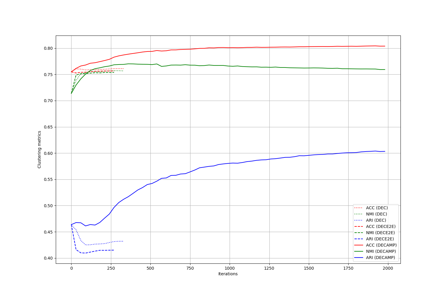
DECAMP performs better than DEC and DECE2E in all three datasets, across all three evaluation metrics. For example, we observed about 4% ACC improvement for DECAMP across all three datasets. We provide detailed metric trajectories along training epochs in Figure ? for one experiment. As can be seen, while DEC and DECE2E’s performance saturate in an early stage, DECAMP continues to improve along iterations till a higher performance level.
- 2.
DEC and DECE2E perform comparably across the datasets. This result was expected in our previous discuss, as neither of them use the graph affinity information in the original space. However, the main advantage of DECE2E is its theoretical elegance and training efficiency, as we can train it end-to-end through a unified loss function.
- 3.
Comparing with other state-of-art methods published on these three datasets, DECAMP is also among the best performers. For example, on Stackoverflow, DECAMP’s ACC is about 5% higher than all existing baselines, including methods using additional information during the clustering process. Notice that on the Biomedical dataset, DECAMP does not compete well with DEC-SIF, and we hypothesize that one reason might be the high-quality word embeddings in DEC-SIF derived from additional in-domain data. For baselines with no access to additional information source (such as DMM-T), we do see a big gain of DECAMP across the board.


Conclusion
In this paper we proposed a new deep clustering method for short text analysis. By combining the strength of deep representation and measure propagation, our DECAMP algorithm uses the neighborhood affinity information to guide the clustering process, and achieves state-of-the-art performance on multiple public datasets. As a by-product, we obtained an end-to-end version of DEC which admits a unified objective function and allows more efficient training. As a future research direction, we will explore the possibility of encoding the measure propagation step as a neural network component, so that DECAMP can become a new kind of graph neural network [\citeauthoryearZhou et al.2018] admitting end-to-end training.
References
- [\citeauthoryearBelkin and Niyogi2003] Belkin, M., and Niyogi, P. 2003. Laplacian eigenmaps for dimensionality reduction and data representation. Neural computation 15(6):1373–1396.
- [\citeauthoryearBelkin, Niyogi, and Sindhwani2006] Belkin, M.; Niyogi, P.; and Sindhwani, V. 2006. Manifold regularization: A geometric framework for learning from labeled and unlabeled examples. Journal of machine learning research 7(Nov):2399–2434.
- [\citeauthoryearChen et al.2016] Chen, X.; Duan, Y.; Houthooft, R.; Schulman, J.; Sutskever, I.; and Abbeel, P. 2016. Infogan: Interpretable representation learning by information maximizing generative adversarial nets. In Advances in neural information processing systems, 2172–2180.
- [\citeauthoryearCsiszár and Tusnády1984] Csiszár, I., and Tusnády, G. 1984. Information geometry and alternating minimization problems. Statistics & Decision, Supplement Issue No 1.
- [\citeauthoryearEvanno, Regnaut, and Goudet2005] Evanno, G.; Regnaut, S.; and Goudet, J. 2005. Detecting the number of clusters of individuals using the software structure: a simulation study. Molecular ecology 14(8):2611–2620.
- [\citeauthoryearGhasedi Dizaji et al.2017] Ghasedi Dizaji, K.; Herandi, A.; Deng, C.; Cai, W.; and Huang, H. 2017. Deep clustering via joint convolutional autoencoder embedding and relative entropy minimization. In Proceedings of the IEEE International Conference on Computer Vision, 5736–5745.
- [\citeauthoryearGoodfellow et al.2014] Goodfellow, I.; Pouget-Abadie, J.; Mirza, M.; Xu, B.; Warde-Farley, D.; Ozair, S.; Courville, A.; and Bengio, Y. 2014. Generative adversarial nets. In Advances in neural information processing systems, 2672–2680.
- [\citeauthoryearGuo et al.2017] Guo, X.; Gao, L.; Liu, X.; and Yin, J. 2017. Improved deep embedded clustering with local structure preservation. In IJCAI, 1753–1759.
- [\citeauthoryearHadifar et al.2019] Hadifar, A.; Sterckx, L.; Demeester, T.; and Develder, C. 2019. A self-training approach for short text clustering. In Repl4NLP, the 4th Workshop on Representation Learning for NLP, 1–6.
- [\citeauthoryearHinton and Salakhutdinov2006] Hinton, G. E., and Salakhutdinov, R. R. 2006. Reducing the dimensionality of data with neural networks. science 313(5786):504–507.
- [\citeauthoryearHinton and Zemel1994] Hinton, G. E., and Zemel, R. S. 1994. Autoencoders, minimum description length and helmholtz free energy. In Advances in neural information processing systems, 3–10.
- [\citeauthoryearHinton2002] Hinton, G. E. 2002. Training products of experts by minimizing contrastive divergence. Neural computation 14(8):1771–1800.
- [\citeauthoryearHu et al.2017] Hu, W.; Miyato, T.; Tokui, S.; Matsumoto, E.; and Sugiyama, M. 2017. Learning discrete representations via information maximizing self-augmented training. In Proceedings of the 34th International Conference on Machine Learning-Volume 70, 1558–1567. JMLR. org.
- [\citeauthoryearJia et al.2015] Jia, K.; Sun, L.; Gao, S.; Song, Z.; and Shi, B. E. 2015. Laplacian auto-encoders: An explicit learning of nonlinear data manifold. Neurocomputing 160:250–260.
- [\citeauthoryearJiang et al.2016] Jiang, Z.; Zheng, Y.; Tan, H.; Tang, B.; and Zhou, H. 2016. Variational deep embedding: An unsupervised and generative approach to clustering. arXiv preprint arXiv:1611.05148.
- [\citeauthoryearKingma and Welling2013] Kingma, D. P., and Welling, M. 2013. Auto-encoding variational bayes. arXiv preprint arXiv:1312.6114.
- [\citeauthoryearKipf and Welling2016] Kipf, T. N., and Welling, M. 2016. Semi-supervised classification with graph convolutional networks. arXiv preprint arXiv:1609.02907.
- [\citeauthoryearKrause, Perona, and Gomes2010] Krause, A.; Perona, P.; and Gomes, R. G. 2010. Discriminative clustering by regularized information maximization. In Advances in neural information processing systems, 775–783.
- [\citeauthoryearKrizhevsky, Sutskever, and Hinton2012] Krizhevsky, A.; Sutskever, I.; and Hinton, G. E. 2012. Imagenet classification with deep convolutional neural networks. In Advances in neural information processing systems, 1097–1105.
- [\citeauthoryearLi, Zhang, and Ouyang2019] Li, X.; Zhang, J.; and Ouyang, J. 2019. Dirichlet multinomial mixture with variational manifold regularization: Topic modeling over short texts. In The AAAI Conference on Artificial Intelligence.
- [\citeauthoryearMin et al.2018] Min, E.; Guo, X.; Liu, Q.; Zhang, G.; Cui, J.; and Long, J. 2018. A survey of clustering with deep learning: From the perspective of network architecture. IEEE Access 6:39501–39514.
- [\citeauthoryearPapadimitrou and Steiglitz1982] Papadimitrou, C. H., and Steiglitz, K. 1982. Combinatorial optimization: algorithms and complexity.
- [\citeauthoryearPrincipe2010] Principe, J. C. 2010. Information theoretic learning: Renyi’s entropy and kernel perspectives. Springer Science & Business Media.
- [\citeauthoryearRoweis and Saul2000] Roweis, S. T., and Saul, L. K. 2000. Nonlinear dimensionality reduction by locally linear embedding. science 290(5500):2323–2326.
- [\citeauthoryearSubramanya and Bilmes2011] Subramanya, A., and Bilmes, J. 2011. Semi-supervised learning with measure propagation. Journal of Machine Learning Research 12(Nov):3311–3370.
- [\citeauthoryearTenenbaum, De Silva, and Langford2000] Tenenbaum, J. B.; De Silva, V.; and Langford, J. C. 2000. A global geometric framework for nonlinear dimensionality reduction. science 290(5500):2319–2323.
- [\citeauthoryearTzoreff, Kogan, and Choukroun2018] Tzoreff, E.; Kogan, O.; and Choukroun, Y. 2018. Deep discriminative latent space for clustering. arXiv preprint arXiv:1805.10795.
- [\citeauthoryearVon Luxburg2007] Von Luxburg, U. 2007. A tutorial on spectral clustering. Statistics and computing 17(4):395–416.
- [\citeauthoryearXie, Girshick, and Farhadi2016] Xie, J.; Girshick, R.; and Farhadi, A. 2016. Unsupervised deep embedding for clustering analysis. In International conference on machine learning, 478–487.
- [\citeauthoryearXu et al.2017] Xu, J.; Xu, B.; Wang, P.; Zheng, S.; Tian, G.; and Zhao, J. 2017. Self-taught convolutional neural networks for short text clustering. Neural Networks 88:22–31.
- [\citeauthoryearYang et al.2017] Yang, B.; Fu, X.; Sidiropoulos, N. D.; and Hong, M. 2017. Towards k-means-friendly spaces: Simultaneous deep learning and clustering. In Proceedings of the 34th International Conference on Machine Learning-Volume 70, 3861–3870. JMLR. org.
- [\citeauthoryearZhou et al.2018] Zhou, J.; Cui, G.; Zhang, Z.; Yang, C.; Liu, Z.; and Sun, M. 2018. Graph neural networks: A review of methods and applications. arXiv preprint arXiv:1812.08434.
- [\citeauthoryearZhu and Ghahramani2002] Zhu, X., and Ghahramani, Z. 2002. Learning from labeled and unlabeled data with label propagation.