Light Curves of Partial Tidal Disruption Events

Many studies indicate that the circularization of the debris is possible due to the general relativistic apsidal precession, which is crucial for the formation of accretion disk (Rees 1988; Hayasaki et al. 2013; Dai et al. 2015; Bonnerot et al. 2015; Bonnerot et al. 2017). Upon each passage of the pericenter, the stream precesses by a small angle $\phi\sim R_{\rm S}/R_{\rm p}$, thus undergoes a succession of self crossings, which dissipates an amount of the specific energy. Consequently, the apocenter of the stream’s new orbit moves closer to the BH, and its eccentricity decreases. The stream crossing is illustrated in Figure 1.

In the $N$-th orbit, the specific energy $\epsilon_{\rm N}$, semi-major axis $a_{\rm N}$, and specific angular momentum $j_{\rm N}$ are related as in: $\epsilon_{\rm N}=GM_{\rm h}/(2a_{\rm N})$, and $j_{\rm N}^{2}=GM_{\rm h}a_{\rm N}(1-e_{\rm N}^{2})$. Under the assumption of completely inelastic collision, the dissipated energy per orbit is (Bonnerot et al. 2017, also see Dai et al. 2015)

assuming the stream’s angular momentum is conserved during the crossings, i.e., $j_{\rm N}=j_{0}$. The dissipated energy during the first crossing is

When the stream is eventually fully circularized, i.e., $e_{N}=0$, then $\epsilon_{\rm N}$ shall take its final value $\epsilon_{\rm c}=GM_{\rm h}/(2R_{\rm c})$, where

is the so-called circularization radius.

We assume that in the circularization phase the energy dissipation mainly comes from the self-collision of the stream. The viscous dissipation is relatively weak during this phase, but it will become important after the circularization (see the discussion in section VIII). Furthermore, we will consider only the part of the stream that is made of the most bound debris, i.e., the “main stream”, since it returns earlier and comprises the major portion of the total stream mass, and neglect the tail of the stream. Due to apsidal precession, this stream crosses and collides with itself in successive orbits, reducing its energy.

Adopting the iterative method in Bonnerot et al. 2017, the specific energy dissipation rate is $\Delta\epsilon_{\rm N}/t_{\rm s,N}$ in the $N$-th orbit, such that the dissipation rate can be estimated by $\Delta M\Delta\epsilon_{\rm N}/t_{\rm s,N}$ during the circularization, where $t_{\rm s,N}$ is the orbital period of $N$-th orbit. Assuming efficient radiative cooling, the luminosity is equal to the dissipation rate, i.e.,

Here we assume the mass of ”main stream” equals to the total fallback mass and neglect the tail of returning stream. The reason is that the main stream contains most of the fallback mass after the first collision, which is approximated to be $\Delta M(1-(4t_{\rm fb}/t_{\rm fb})^{-5/4})\simeq 0.82\ \Delta M$ by assuming $\dot{M}_{\rm fb}\propto(t/t_{\rm fb})^{-9/4}$ (Coughlin & Nixon 2019; Miles et al. 2020).

The mass of the main stream is very sensitive to $\beta$. When $\beta>0.5$ the tidal disruption occurs (Ryu et al. 2020a). In this paper, we calculate three cases of PTDEs with $\beta=0.55,0.6,0.7$, whose total fallback mass are $\Delta M\simeq 0.0048,0.0254,0.1222\ M_{*}$, respectively (Guillochon & Ramirez-Ruiz 2013).

Alternatively, we can write the energy dissipation rate history in a differential form: $\dot{\epsilon}(t)=d\epsilon/dt=\Delta\epsilon_{\rm N}/t_{\rm s,N}$. Substituting the orbital period-energy relation $t_{\rm s,N}\equiv 2\pi GM_{\rm h}/(2\epsilon_{\rm N})^{3/2}$ and Equation (5), we get a differential equation of $\epsilon$:

When $a_{\rm N}\gg R_{\rm c}$, $\epsilon/\epsilon_{\rm c}\ll 1$, the factor $1-\epsilon/\epsilon_{\rm c}$ can be dropped, then one can determine the time-scale of circularization by solving for $\epsilon(t)$ from the above equation. Letting $e_{0}\sim 1$, we obtain the circularization time-scale

for PTDEs. The same formula was obtained in Bonnerot et al. 2017 along a different approach.

For the PTDE with $\beta=0.5$, it needs to spend a duration $\sim 16\ t_{\rm fb}$ to form a circular disk. Other mechanism, e.g. the magneto-rotational instability (MRI), may cause momentum exchange and speed up the circularization process (Bonnerot et al. 2017; Chan et al. 2018). We assume the viscous effects are weak in the circularization stage. We will further explore this issue in section VIII.

Furthermore, from Equation (9) it is straightforward to find that the peak dissipative luminosity per mass is

Then using Equation (2) and (6), we get the peak luminosity

Using the differential form, i.e., Equation (9), we can rewrite the circularization luminosity as $L_{\rm c}(t)\simeq\Delta M\dot{\epsilon}(t)$ and plot it in Figure 2. The result of this differential form is equivalent to that of iterative form (Equation (8)), and it provides a clear relation between the parameters, hence we adopt it in the following calculations.

The luminosity estimate above assumes that photons can diffuse efficiently. However, we should examine the issue of diffusion efficiency more carefully. After the self-collision, the gas is heated, the photon needs some time to diffuse out. The diffusion time-scale determines the observed luminosity and the spectrum. If the diffusion time-scale is much shorter than the orbital period, the radiation mainly emerges from the stream near the collision position. Otherwise, the thermal energy will be accumulated during the circularization process.

The radiative diffusion time-scale after the shock is given by $t_{\rm diff}\simeq\tau h_{\rm s}/c$, where $c$ and $h_{\rm s}$ are the light speed and the height of the stream, respectively. And the optical depth of the stream after the shock is $\tau\simeq\kappa_{\rm es}\rho h_{\rm s}$, where $\kappa_{\rm es}\simeq 0.34\ {\rm cm^{2}\ g^{-1}}$ is the opacity for electron scattering for a typical stellar composition ²² 2 The atoms are ionized after the shock, and the temperature is high, so that the electron scattering dominates the opacity..

Assuming the stream is homogeneous in the interior, the density of the stream after the shock is estimated by

Here $w_{\rm s}$ is the width of the stream. And the perimeter of the orbit is $\sim 4a_{\rm s}$, where $a_{\rm s}$ is the semi-major axis of the orbit. Then the diffusion time-scale after the shock can be written as

where $t_{\rm s}$ is the orbital period of the stream. In order to estimate the evolution of diffusion time-scale during the circularization process, we need to consider the evolution of the apocenter radius and the height-to-width ratio of the stream.

The apocenter radius becomes smaller as the circularization process carries on. The change of height-to-width is complicated, since it evolves under the gravity and pressure force. In Bonnerot et al. 2017, they assume $h_{\rm s}/w_{\rm s}=1$ during the circularization process. We should relax this assumption here, because the SMBH’s gravity will restrict the expansion of stream in the vertical direction, and the width of stream increases slightly due the viscous shear. Therefore, when the stream is cold at later times, the stream will become geometrically thin (Bonnerot et al. 2015), so the height-to-width ratio should be $h_{\rm s}/w_{\rm s}\ll 1$.

We set $h_{\rm s}/w_{\rm s}\simeq 1$ at the beginning of the circularization process, and let $h_{\rm s}/w_{\rm s}\simeq 10^{-2}$ when the circularization process completes, which is consistent with the geometrically thin ring (or disk) (Kato et al. 1998). To account for a smooth transition we adopt the following form for the evolution of the height-to-width ratio

We show the history of $t_{\rm diff}/t_{\rm s}$ in Figure 3. It shows that the radiative diffusion is efficient during the whole circularization process for $\beta\sim 0.5$, but not for $\beta\sim 0.9$.

If the radiative diffusion is efficient, i.e. $t_{\rm diff}\lesssim t_{\rm s}$, then the thermal energy will not be accumulated in each orbit. At the early time when $a_{\rm s}\sim a_{\rm 0}$, the photon can diffuse out efficiently before the next shock for PTDEs. However, for those FTDEs with $\beta\gtrsim\beta_{\rm d}$, the bound mass $\Delta M\sim 0.5\ M_{\odot}$, the diffusion time-scale $t_{\rm diff}\gtrsim t_{\rm s}$ and thus the photon cannot diffuse efficiently.

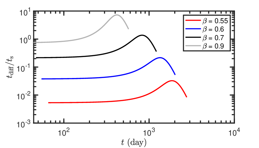
Since we focus on the PTDEs, the assumption of efficient radiative cooling is reasonable. Therefore we do not consider the photon diffusion in the calculations of the luminosity of circularization hereafter.

The energy balance during the viscous evolution is given by $Q^{+}=Q^{-}_{\rm adv}+Q^{-}_{\rm rad}$. Here the viscous heating rate per unit surface area is

The radiative cooling rate is

and the advective term is given by

where $\dot{M}_{\rm acc}=3\pi\nu\Sigma$ is the local accretion rate and $\xi$ is close to unity (Frank et al. 1985). Here $\Sigma$, $\Omega$, $a$, and $T_{\rm c}$ are the local surface density, the local angular velocity, radiation constant, and the mid-plane temperature, respectively.

The total pressure is $P_{\rm tot}=P_{\rm rad}+P_{\rm gas}=aT_{\rm c}^{4}/3+\rho k_{\rm b}T_{\rm c}/(\mu m_{\rm p})$. Here $k_{\rm b}$, $\mu=0.6$, and $m_{\rm p}$ are the Boltzmann constant, mean particle weight, and proton mass, respectively. The local density is $\rho\simeq\Sigma/(2H)$. Here the height-scale is given by the hydrostatic equilibrium, i.e.,

We adopt the $\alpha_{\rm g}$-viscosity (Sakimoto & Coroniti 1981), i.e.,

to calculate the viscous evolution.

The local opacity is $\kappa=\kappa_{\rm es}+\kappa_{\rm R}$, where the electron scattering opacity is dominated by Thompson electron scattering, i.e., $\kappa_{\rm es}=0.2(1+X)\ {\rm cm^{2}g^{-1}}$, and the Kramer’s opacity is given by $\kappa_{\rm R}=4\times 10^{25}Z(1+X)\rho T^{-3.5}\ {\rm cm^{2}g^{-1}}$. The gas composition we adopt in this paper is the solar composition, i.e., $X=0.71$, $Y=0.27$, and $Z=0.02$.

The viscous evolution was considered by Cannizzo et al. 1990, and we summarize it here. We assume the disk is in thermal equilibrium between viscous heating and radiative cooling, i.e., $Q^{+}=Q^{-}_{\rm rad}$. Using these relations we obtain the temperature

The viscous time-scale is given by

It is the function of time and radius, but we can average it with respect to $R$ by letting $R=R_{\rm d}$ and $\Sigma=\Delta M/(2\pi R_{\rm d}^{2})$, where $R_{\rm d}$ is the average radius of the disk (ring). Substituting the average surface density and radius into Equation (21), and using Equations (20) and (22), we obtain

where $M_{\rm d}$ is the total mass of the disk (ring).

At the beginning $R_{\rm d}=R_{\rm c}$ and $M_{\rm d}=\Delta M$, the initial viscous time-scale is

which is the time-scale of the ring-to-disk phase. Notice that the ring-to-disk time-scale does not depend on the initial width of the ring.

In order to estimate the bolometric luminosity, we assume the accretion rate is

and keep the total angular momentum $J_{\rm d}=M_{\rm d}(GM_{\rm h}R_{\rm d})^{1/2}$ constant during the ring-to-disk and disk phase (Kumar et al. 2008), i.e.,

Then Equation (23) becomes $t_{\nu}=t_{0}(M_{\rm d}/\Delta M)^{-16/3}$. Substituting it into Equation (25) and assuming a constant opacity, one obtains the accretion rate

The bolometric luminosity can be written as $L_{\rm disk}=\eta\dot{M}_{\rm acc}c^{2}$. The efficiency is $\eta=1/12$ for Schwarzschild BH. We plot it in Figure 4 with the electron scattering assumption $\kappa=\kappa_{\rm es}$ to compare with the numerical results. According to the results in Figure 4, we can estimate the peak luminosity in viscous evolution by

When $t\gtrsim t_{0}$, the luminosity is $\propto t^{-1.2}$, which is same as the self-similar result in Cannizzo et al. 1990. Notice that the early part ($t<t_{0}$) of the solution is a rough approximation, because at this stage the accretion rate in Equation (27) is not necessarily the mass inflow rate at the inner boundary of the disk (i.e., near the BH’s event horizon) due to a likely viscous diffusion delay. A more rigorous way to explore this early phase is described below.

The viscous evolution is governed by the diffusion equation of the surface density (Frank et al. 1985), i.e.,

We list the assumptions and initial conditions of the numerical model here:

• •

  We assume the ring is axisymmetric with a Gaussian surface density profile centered at the circularization radius $R_{\rm c}$

  $$\Sigma(R)=\zeta\frac{\Delta M}{R_{\rm c}w_{0}}{\rm exp}\left[-\left(\frac{R-R_{\rm c}}{2w_{0}}\right)^{2}\right],$$

  (30)

  where $\zeta\simeq 1/(4\pi^{3/2})$ is a coefficient that satisfies

  $$\int^{\infty}_{R_{\rm in}}\Sigma(R)2\pi R\ dR=\Delta M.$$

  (31)

  We set the initial width of the ring as $w_{0}=0.1R_{\rm c}$.

• •

  We set the inner boundary condition to be $R_{\rm in}=R_{\rm ISCO}=3R_{\rm S}$ corresponding to a Schwarzschild BH. Once the matter arrives the boundary, it is removed.

• •

  For simplicity we adopt the vertically-averaged disk (ring), and neglect the returning stream $\dot{M}_{\rm fb}$ after the circularization, so we only calculate the 1D evolution.

• •

  We consider the form of advective cooling term is Equation (18). However, it is important only if the accretion rate is super-Eddington (Shen & Matzner 2014).

• •

  We use the $\alpha_{\rm g}$-viscosity ansatz, i.e., Equation (20), to avoid the thermal instability (Lightman & Eardley 1974). Moreover, because the fitting results of TDEs in van Velzen et al. 2019 give the high viscosity, i.e., $\alpha>0.1$, we set $\alpha=1$ in the following calculations.

We show the results of the evolution of the surface density in Figure 5. We can see the time-scales of the ring-to-disk phase are consistent with the analytical calculation in section IV.2. Even though the opacity in the numerical calculation is not a constant, the time-scale $t_{0}$, i.e., Equation (24) depends weakly on $\kappa$, so $t_{0}$ is a good approximation of the time-scale of ring-to-disk phase.

The emergent energy flux is given by

where $\sigma$ and $T_{\rm eff}$ are the Stefan-Boltzmann constant and local effective temperature, respectively. The factor $1/2$ comes form the two side of the disk (ring). The bolometric luminosity is given by

and is shown in Figure 4. After the formation of accretion disk, the numerical results approach the self-similar ones. However, the analytical results overestimate the luminosity in the ring-to-disk phase.

For an observer at distance $D$ whose viewing angle is $i$, with the blackbody assumption the flux at wavelength $\lambda$ is given by

where the Planck function $B_{\lambda}$ is

and $h$ is the Planck constant.

The evolution of local effective temperatures and that of the spectrum are shown in Figure 6 and 7, respectively. We use the peak local effective temperature $\max[T_{\rm eff}(R)]$ to represent the observed effective temperature of the whole disk surface, and plot its evolution in Figure 8.

During the circularization process, we assume most of the radiation comes from the shocked region, and the shocked matter-radiation mixture is thermalized. Here we estimate the effective temperature by the single blackbody assumption

and assume the viewing angle is face-on. We determine the radiative area $S$ by considering the diffusion time-scale as below.

When the radiative diffusion is efficient, i.e., $t_{\rm diff}\lesssim t_{\rm s}$, the initial radiative area $S_{0}$ can be written as the product of the width and the length of the radiative region:

Here the length can be estimated by $l_{\rm diff,0}\sim v_{\rm a,0}t_{\rm diff,0}$, and $v_{\rm a,0}\simeq(GM_{\rm h}/a_{0})^{1/2}((1-e_{0})/(1+e_{0}))^{1/2}$ is the stream velocity near the opocenter.

We assume the initial expansion of stream is ballistic after the collision, thus the width is $w_{\rm s,0}\simeq R_{0}+c_{\rm s,0}t_{\rm diff,0}$, where $R_{0}$ is the initial width of the stream near the collision point and the sound speed after the collision is $c_{\rm s,0}\simeq 2/3\Delta\epsilon_{0}^{1/2}$. For PTDEs, the self-gravity is negligible. Before the collision, the stream width is dominated by the tidal shear, thus in this limit $R_{0}\simeq R_{*}(a_{0}/R_{\rm p})$ (Kochanek 1994; Coughlin et al. 2016).

If $c_{\rm s,0}t_{\rm diff,0}\gg R_{0}$, then it is the former that determines $w_{\rm s,0}$. We can estimate the initial radiative area as

where we use Equations (3), (6) and (14) and assume an initial $h_{\rm s}/w_{\rm s}\simeq 1$.

After the collisions, the orbital energy will be redistributed gradually, causing the stream to extend slightly in the radial direction. Furthermore, the viscous shear in the late stage of the circularization grows, further widening the stream. It is difficult to obtain the detailed evolution of the radiative area by an analytical method. Instead, we parametrize the radiative area evolution in a smooth power-law form

where $1.5\ t_{\rm fb}$ is the time when the first collision occurs. The power law index $\gamma$ is determined by the starting condition of the disk viscous evolution (see below).

In order to obtain the whole light curve including the circularization stage and the disk viscous evolution stage, we connect the luminosity curves of the two stages at an intermediate point where these two are equal, as is shown in Figure 9. After this transition time $t_{\rm c}$, the disk viscous evolution dominates the luminosity.

So far we have assumed the emission spectrum is a single blackbody in the circularization stage and a multi-color blackbody in the disk viscous evolution stage. Thus there are some uncertainties in the transition between the two. In fact, if the initial width of the circularized ring at the beginning of the second stage is small, the spectrum is approximate to a single blackbody as well. Therefore, we expect that the effective temperature should vary smoothly during the transition. Therefore, the radiative area evolution index $\gamma$ during the circularization process can be determined by

Here $S_{\rm c}=L_{\rm disk}/(\sigma\max[T_{\rm eff}(R)]^{4})$ is the effective radiative area at the transition time $t_{\rm c}$ when the luminosity of the viscous evolution becomes dominating the luminosity.

With these, the overall evolution of the effective temperature for the entire PTDE can be calculated and is plotted in Figure 10.

The parameter space for PTDEs and FTDEs are $0.5<\beta<\beta_{\rm d}$ and $\beta_{\rm d}<\beta<\beta_{\rm max}$, respectively. The exact value of $\beta$ for the partial disruption onset is $\beta>0.5$ (Ryu et al. 2020a).The upper limit of the penetration factor for disruption $\beta_{\rm max}$ is given by $\beta_{\rm max}\simeq R_{\rm T}/R_{\rm S}$. If $\beta>\beta_{\rm max}$, SMBH will directly swallow the whole star instead of tidally disrupting it (Kesden 2012). Notice that if $\beta_{\rm max}<\beta_{\rm d}$, only PTDEs can occur in that case.

We can estimate the event rate of TDEs by the loss-cone dynamics (Merritt 2013). Occasionally a star will be scattered into a highly eccentric orbit with pericenter radius $R_{\rm p}\lesssim R_{\rm lc}\equiv\max[R_{\rm S},R_{\rm d}]$, and the star will be captured or fully disrupted by the SMBH. Here $R_{\rm d}=R_{\rm T}/\beta_{\rm d}$ is the full disruption radius. The rate of the stars entering $R_{\rm lc}$ (hereafter as $\dot{N}_{\rm lc}$) depends on the realistic stellar density profile in the nucleus of each galaxy. In Stone & Metzger 2016, they use an early-type galaxy sample consisting of 144 galaxies to calculate the TDE rate. Here we use their fitting result (Eq. 27 in Stone & Metzger 2016), i.e.,

with $\dot{N}_{0}=2.9\times 10^{-5}\ \rm{yr^{-1}gal^{-1}}$ and $B=-0.404$, to estimate the stellar loss rate in a galaxy.

Using the loss rate $\dot{N}_{\rm lc}$, the fraction function of SMBHs $\phi(M_{\rm h})$, the fraction function of penetration factor $f_{\rm TDE}$, and the initial mass function (IMF) $\chi_{\rm Kro}$ in Appendix A, one can calculate the differential volumetric event rates of PTDEs and FTDEs with respect to the SMBH mass by

where $m_{*,{\rm min}}$ is the lower limit for TDE, it is given by Eq. (A4).

The volumetric event rates of TDEs with respect to $M_{\rm h}$ is shown in Fig. 15. The structure of polytropic stars with $\gamma=4/3$ are denser than that with $\gamma=5/3$, therefore it needs to be much closer to the SMBH for full disruptions, thus reducing the probability for FTDEs.

The event rates of PTDE and FTDE are similar for the smaller SMBHs $M_{\rm h}\leq 10^{6}\ M_{\odot}$. However, the event rate of PTDEs becomes dominant for the larger SMBHs. There are two reasons: First, the radius for the full disruption become closer to the SMBH as the SMBH mass increases, when $M_{\rm h}>10^{8}\ M_{\odot}$ the stars can not be fully disrupted, then only PTDEs can occur. Second, most of the stars are in the diffusion limit for the lager SMBHs (see Eq. (A5)), which will suppress the FTDEs.

Overall, the chance of PTDEs is very promising. The event rate of PTDEs is greater than that of FTDEs, even for the larger SMBHs. Notice that Ryu et al. 2020a consider the realistic stellar structure by using MESA, and find that for low-mass stars the chance of PTDEs is approximately equal to that of FTDEs, but for high-mass star, the likelihood of PTDEs is 4 times higher than that of FTDEs. However, they consider only the full loss-cone regime and neglect the upper limit of penetration $\beta_{\rm max}$ for FTDEs. Therefore, their estimate of the PTDE fraction is lower than ours.

The fallback mass of PTDE is less than that of FTDE, so PTDE is seemingly dimmer than FTDE. However, as we discuss above, PTDEs prefer heavier SMBHs, thus most of them are bright and detectable. The detection rate depends on the physical processes that contribute to the emission of TDEs (Stone & Metzger 2016). Here we calculate the detection rate of PTDEs using our model.

The limiting detection distance for a PTDE is

where the spectral flux density limit $f_{\nu}$ is given by $m_{\rm R}\simeq-2.5\ \lg(f_{\nu}/3631\rm{J_{y}})$ and the R-band limiting magnitude $m_{R}\simeq 20.5$ for ZTF. The monochromatic luminosity of the source is $L_{\nu}\simeq\pi B_{\nu}(T_{\rm eff})S$, where $B_{\nu}$ is the Planck function. The effective temperature $T_{\rm eff}\sim(L_{\rm p}/(\sigma S_{0}))^{1/4}$ and radiative area $S\sim S_{0}$ are given in the model, i.e., Eq. (12) and (38), thus $d_{\rm lim}$ is the function of $\beta$, $M_{\rm h}$ and $m_{*}$.

The detection rate of PTDEs is

Here $\beta_{\rm lc}\equiv R_{\rm T}/R_{\rm lc}$. The integral upper limit of the SMBH mass is given by $R_{\rm T}/0.5=R_{\rm S}$, i.e., $M_{\rm h,max}=(R_{\odot}c^{2}/(GM_{\odot}^{1/3}))^{3/2}$.

It gives $D_{\rm p}\sim 5\times 10^{2}\ {\rm yr^{-1}}$ for $\gamma=5/3$, and $D_{\rm p}\sim 10^{2}\ {\rm yr^{-1}}$ for $\gamma=4/3$. Taking the field of view of ZTF into consideration ($\sim 0.1$ of the whole sky), the ZTF detection rate of PTDEs is about dozens per year.

In the calculation of the circularization process, we neglect the viscous effects. Here we explore the importance of viscous effects in the circularization stage. There are two main effects of the viscous shear. One is that the viscous shear can heat up the stream and increase the luminosity. Furthermore, the viscous shear can redistribute the angular momentum of the debris stream and cause some parts of the stream to be closer to the SMBH. Then it may further enhance the dissipation caused by the viscous shear and the self-crossing, and speeds up the formation of the disk (elliptical or circular disk).

Svirski et al. 2017 (Bonnerot et al. 2017, also see) calculate the viscous effects induced by the magnetic stress, which originates from the exponential growth of the magneto-rotational instability (MRI) (Balbus & Hawley 1991). In order to be consistent with the prescription of viscosity adopted in the disk stage, we also adopt the $\alpha_{\rm g}$-viscosity (Equation (20)) to parametrize the viscous shear in the circularization stage.

One can find that the prescription of $\alpha_{\rm g}$-viscosity is equivalent to that of magnetic stress used in Svirski et al. 2017 if we let $\alpha\simeq\alpha_{\rm mag}(v_{\rm A}/c_{\rm s})^{2}$. Here $\alpha_{\rm mag}$ and $v_{\rm A}$ are the ratio of the $\hat{n}-\hat{t}$ magnetic stress component to the total magnetic stress and the Alfvén velocity, respectively.

The redistribution of the specific angular momentum caused by the viscous shear can be estimated by $dj/dt\simeq\nu\Omega$. The total change of the specific angular momentum during the circularization process can be written as $\Delta j\simeq\nu\Omega t_{\rm cir}$, thus

where the specific angular momentum is $j\simeq(GM_{\rm h}R_{\rm c})^{1/2}$. For PTDEs with $M_{\rm h}\gtrsim 10^{6}\ M_{\odot}$, the viscous shear has negligible effect on the extension of stream during the circularization process. Therefore the structure of stream will keep thin until its orbit circularizes and settles into a ring.

Another viscous effect is that it can heat up the stream and increase the luminosity. We can estimate the viscous luminosity in the circularization process by assuming the viscous heating rate equals to the radiative cooling rate, i.e., $L_{\rm c,vis}\simeq\int\nu\Omega^{2}\Sigma\ dS$. Most of the viscous heating come from the pericenter where only a small part of the stream mass locates at, thus the viscous luminosity is very small, i.e., $L_{\rm c,vis}\ll(\nu\Omega^{2})_{\rm p}\Delta M\simeq L_{\rm disk,0}$. Here the subscript $p$ denotes the value at the pericenter radius, and $L_{\rm disk,0}$ is the luminosity of the ring after the circularization process.

Therefore, it is reasonable to neglect the viscous effects in the circularization process. In the late time of the circularization, the viscous effects become important and the luminosity is dominated by the viscous shear.

In the transition between the circularization stage and the viscous evolution stage, we artificially connect the light curve of these two stages due to the fact that the luminosity induced by the viscous shear is small in the circularization stage. In fact the transition should be smooth if we take the viscous heating into account in the circularization stage.

We consider that in the circularization stage most of the radiation comes from the shock-heated debris stream. As the material cools down, the ions will recombine. Assuming most of the material is hydrogen, the total recombination energy is $E_{\rm re}\simeq N\times 13.6\ {\rm eV}\simeq 3\times 10^{44}\ (\Delta M/0.01\ M_{\odot})\ {\rm erg}$, where $N$ is the number of hydrogen ions. The recombination luminosity is $L_{\rm re}\simeq E_{\rm re}/t_{\rm fb}\simeq 10^{38}\ {\rm erg/s}$, which is negligible. Recombination will probably promote the chemical reactions in the stream, so that dust clumps form (Kochanek 1994). However, these dust will be evaporated in later shocks.

We calculate the detection rate of PTDEs through loss-cone dynamic. For ZTF, the detection rate is about dozens per year, it is very promising. We encourage the search of them by optical/UV or soft X-ray telescopes. For some PTDEs that might have already been discovered in the past data, our work would be useful to identify them.

Recently, Gomez et al. 2020 report a TDE candidate AT 2018hyz. They use the Modular Open-Source Fitter for Transients (MOSFIT) to model the light curves, and conclude that it is a PTDE. The MOSFIT model assumes a rapid circularization of the stream and that the evolution of luminosity traces the mass fallback rate, which may not be the case for PTDEs, as we have shown. The double peaks in the light curve of AT 2018hyz are consistent with what we predict for a PTDE, which is the feature of a two-stage evolution.

However, the blackbody spectral fitting of AT 2018hyz gives a large photosphere $\sim 10^{15}\ {\rm cm}$, which is not consistent with our model. There are some uncertainty in the spectrum fitting, e.g., the galaxy extinction and prior spectrum assumption. Furthermore, in the circularization process, the spectrum might deviate from the blackbody spectrum we assume here. More details of the radiative dynamical evolution of the circularization need to be understood.

Recently, Frederick et al. 2020 report five transient events found by ZTF from active galactic nucleus (AGNs). One of them, ZTF19aaiqmgl, shows two peaks in the light curve, and only the second peak has X-ray detection. The second peak might correspond to the disk formation. However, in an AGN, the debris from the disrupted star will collide with the pre-existing accretion disk (Chan et al. 2019), and the shocks will heat up the gas. For PTDEs, the lighter streams might directly merge with the disk. The details of PTDEs from AGNs are still unclear.

Furthermore, Payne et al. 2021 report a repeated PTDE candidate ASASSN-14ko, which is located within an AGN. The star will be tidally stripped by the BH during each encounter near the pericenter, if the star is in an elliptical orbit. The pre-existing accretion disk can produce periodic bright flares by accreting these stripped mass. Thus the debris might not experience a long-term circularization and disk formation process, but how the debris interact with the pre-existing disk is unclear.

References

- Balbus & Hawley (1991) Balbus, S. A., & Hawley, J. F. 1991, ApJ, 376, 214, doi: 10.1086/170270
- Bonnerot et al. (2017) Bonnerot, C., Rossi, E. M., & Lodato, G. 2017, MNRAS, 464, 2816, doi: 10.1093/mnras/stw2547
- Bonnerot et al. (2015) Bonnerot, C., Rossi, E. M., Lodato, G., & Price, D. J. 2015, MNRAS, 455, 2253, doi: 10.1093/mnras/stv2411
- Cannizzo et al. (1990) Cannizzo, J. K., Lee, H. M., & Goodman, J. 1990, ApJ, 351, 38, doi: 10.1086/168442
- Chan et al. (2018) Chan, C.-H., Krolik, J. H., & Piran, T. 2018, ApJ, 856, 12, doi: 10.3847/1538-4357/aab15c
- Chan et al. (2019) Chan, C.-H., Piran, T., Krolik, J. H., & Saban, D. 2019, ApJ, 881, 113, doi: 10.3847/1538-4357/ab2b40
- Coughlin et al. (2016) Coughlin, E. R., Nixon, C., Begelman, M. C., & Armitage, P. J. 2016, MNRAS, 459, 3089, doi: 10.1093/mnras/stw770
- Coughlin & Nixon (2019) Coughlin, E. R., & Nixon, C. J. 2019, ApJ, 883, L17, doi: 10.3847/2041-8213/ab412d
- Dai et al. (2015) Dai, L., McKinney, J. C., & Miller, M. C. 2015, ApJ, 812, L39, doi: 10.1088/2041-8205/812/2/l39
- Frank et al. (1985) Frank, J., King, A. R., & Raine, D. J. 1985, Accretion power in astrophysics (Cambridge: University Press). https://ui.adsabs.harvard.edu/abs/1985apa..book.....F
- Frederick et al. (2020) Frederick, S., Gezari, S., Graham, M. J., et al. 2020, arXiv:2010.08554. https://ui.adsabs.harvard.edu/abs/2020arXiv201008554F
- Gezari et al. (2012) Gezari, S., Chornock, R., Rest, A., et al. 2012, Nature, 485, 217, doi: 10.1038/nature10990
- Gomez et al. (2020) Gomez, S., Nicholl, M., Short, P., et al. 2020, MNRAS, 497, 1925, doi: 10.1093/mnras/staa2099
- Guillochon & Ramirez-Ruiz (2013) Guillochon, J., & Ramirez-Ruiz, E. 2013, ApJ, 767, doi: 10.1088/0004-637x/767/1/25
- Hayasaki et al. (2013) Hayasaki, K., Stone, N., & Loeb, A. 2013, MNRAS, 434, 909, doi: 10.1093/mnras/stt871
- Holoien et al. (2014) Holoien, T. W. S., Prieto, J. L., Bersier, D., et al. 2014, MNRAS, 445, 3263, doi: 10.1093/mnras/stu1922
- Holoien et al. (2016) Holoien, T. W. S., Kochanek, C. S., Prieto, J. L., et al. 2016, MNRAS, 455, 2918, doi: 10.1093/mnras/stv2486
- Jiang et al. (2016) Jiang, Y.-F., Guillochon, J., & Loeb, A. 2016, ApJ, 830, 125, doi: 10.3847/0004-637x/830/2/125
- Kato et al. (1998) Kato, S., Fukue, J., & Mineshige, S. 1998, Black-hole accretion disks (Kyoto, Japan: Kyoto University Press). https://ui.adsabs.harvard.edu/abs/1998bhad.conf.....K
- Kesden (2012) Kesden, M. 2012, Physical Review D, 85, 024037, doi: 10.1103/PhysRevD.85.024037
- Kochanek (1994) Kochanek, C. S. 1994, ApJ, 422, 508, doi: 10.1086/173745
- Kochanek (2016) —. 2016, MNRAS, 461, 371, doi: 10.1093/mnras/stw1290
- Kroupa (2001) Kroupa, P. 2001, MNRAS, 322, 231, doi: 10.1046/j.1365-8711.2001.04022.x
- Kumar et al. (2008) Kumar, P., Narayan, R., & Johnson, J. L. 2008, MNRAS, 388, 1729, doi: 10.1111/j.1365-2966.2008.13493.x
- Law-Smith et al. (2020) Law-Smith, J. A. P., Coulter, D. A., Guillochon, J., Mockler, B., & Ramirez-Ruiz, E. 2020, ApJ, 905, 141, doi: 10.3847/1538-4357/abc489
- Lightman & Eardley (1974) Lightman, A. P., & Eardley, D. M. 1974, ApJ, 187, L1, doi: 10.1086/181377
- Liu et al. (2020) Liu, F., Cao, C., Abramowicz, M. A., et al. 2020, arXiv:2012.05552. https://ui.adsabs.harvard.edu/abs/2020arXiv201205552L
- Lodato et al. (2009) Lodato, G., King, A. R., & Pringle, J. E. 2009, MNRAS, 392, 332, doi: 10.1111/j.1365-2966.2008.14049.x
- Lodato & Rossi (2011) Lodato, G., & Rossi, E. M. 2011, MNRAS, 410, 359, doi: 10.1111/j.1365-2966.2010.17448.x
- Lu & Bonnerot (2020) Lu, W., & Bonnerot, C. 2020, MNRAS, 492, 686, doi: 10.1093/mnras/stz3405
- Mainetti et al. (2017) Mainetti, D., Lupi, A., Campana, S., et al. 2017, A&A, 600, doi: 10.1051/0004-6361/201630092
- Manukian et al. (2013) Manukian, H., Guillochon, J., Ramirez-Ruiz, E., & O’Leary, R. M. 2013, ApJ, 771, L28, doi: 10.1088/2041-8205/771/2/l28
- McConnell & Ma (2013) McConnell, N. J., & Ma, C.-P. 2013, ApJ, 764, 184, doi: 10.1088/0004-637x/764/2/184
- Merritt (2013) Merritt, D. 2013, CQGra, 30, 244005, doi: 10.1088/0264-9381/30/24/244005
- Metzger & Stone (2016) Metzger, B. D., & Stone, N. C. 2016, MNRAS, 461, 948, doi: 10.1093/mnras/stw1394
- Miles et al. (2020) Miles, P. R., Coughlin, E. R., & Nixon, C. J. 2020, ApJ, 899, 36, doi: 10.3847/1538-4357/ab9c9f
- Miller et al. (2015) Miller, B. P., Gallo, E., Greene, J. E., et al. 2015, ApJ, 799, 98, doi: 10.1088/0004-637x/799/1/98
- Payne et al. (2021) Payne, A. V., Shappee, B. J., Hinkle, J. T., et al. 2021, ApJ, 910, 125, doi: 10.3847/1538-4357/abe38d
- Phinney (1989) Phinney, E. S. 1989, IAUS, 136, 543. https://ui.adsabs.harvard.edu/abs/1989IAUS..136..543P
- Piran et al. (2015) Piran, T., Svirski, G., Krolik, J., Cheng, R. M., & Shiokawa, H. 2015, ApJ, 806, 164, doi: 10.1088/0004-637x/806/2/164
- Ramirez-Ruiz & Rosswog (2009) Ramirez-Ruiz, E., & Rosswog, S. 2009, ApJ, 697, L77, doi: 10.1088/0004-637x/697/2/l77
- Rees (1988) Rees, M. J. 1988, Nature, 333, 523, doi: 10.1038/333523a0
- Ryu et al. (2020a) Ryu, T., Krolik, J., Piran, T., & Noble, S. C. 2020a, ApJ, 904, 98, doi: 10.3847/1538-4357/abb3cf
- Ryu et al. (2020b) —. 2020b, ApJ, 904, 100, doi: 10.3847/1538-4357/abb3ce
- Sakimoto & Coroniti (1981) Sakimoto, P. J., & Coroniti, F. V. 1981, ApJ, 247, 19, doi: 10.1086/159005
- Schechter (1976) Schechter, P. 1976, ApJ, 203, 297, doi: 10.1086/154079
- Shen & Matzner (2014) Shen, R.-F., & Matzner, C. D. 2014, ApJ, 784, doi: 10.1088/0004-637x/784/2/87
- Shiokawa et al. (2015) Shiokawa, H., Krolik, J. H., Cheng, R. M., Piran, T., & Noble, S. C. 2015, ApJ, 804, 85, doi: 10.1088/0004-637x/804/2/85
- Stone & Metzger (2016) Stone, N. C., & Metzger, B. D. 2016, MNRAS, 455, 859, doi: 10.1093/mnras/stv2281
- Strubbe & Quataert (2009) Strubbe, L. E., & Quataert, E. 2009, MNRAS, 400, 2070, doi: 10.1111/j.1365-2966.2009.15599.x
- Svirski et al. (2017) Svirski, G., Piran, T., & Krolik, J. 2017, MNRAS, 467, 1426, doi: 10.1093/mnras/stx117
- Torres et al. (2010) Torres, G., Andersen, J., & Giménez, A. 2010, A&AR, 18, 67, doi: 10.1007/s00159-009-0025-1
- van Velzen et al. (2019) van Velzen, S., Stone, N. C., Metzger, B. D., et al. 2019, ApJ, 878, 82, doi: 10.3847/1538-4357/ab1844