We take equation (3.16) and solve it by postulating the following solution:

$\displaystyle e^{\imath N\tilde{S}_{+}(P,w)}=\frac{\theta(P>0)e^{-\imath NPw}}{1-e^{\imath N(\varphi_{+}(w)+\imath cP)}},\quad{\rm Im}(w)>0,$

(3.17)

where $\varphi_{\pm}$ are the analytic continuation of $\varphi$ from above or below the real axis, respectively. $\varphi$ has a jump discontinuity at the support of the Bethe roots, so that we have two different analytical continuations through the cut depending on whether one comes from above or below the real axis. In the end we shall take $w$ to be real, so that in the final equations for the matrix elements, $\varphi_{\pm}(w),$ will simply denote $\varphi(w\pm\imath 0^{+}),$ respectively.

Actually what we meant by Eq. (3.17) is that there are two asymptotes:

$\displaystyle e^{\imath N\tilde{S}_{+}(P,w)}=\begin{cases}-e^{-\imath N(\varphi_{+}(w)+(w+\imath c)P)}&0<P<-\frac{1}{c}{\rm Im}(\varphi_{+}(w))\\ e^{-\imath NPw}&0<-\frac{1}{c}{\rm Im}(\varphi_{+}(w))<P\\ \end{cases}.$

(3.18)

Performing the inverse Fourier transform on this object one obtains the following form for ${R}(z,w)$:

$\displaystyle R(z,w)=\frac{e^{\frac{\imath N}{c}(z-w){\rm Im}\varphi_{+}(w)}}{z-w}.$

(3.19)

Here only $P$ values above $-\frac{{\rm Im}(\varphi_{+}(w))}{c}$ were taken into account (the second line on the right hand side of Eq. (3.18)), since values of $P$ lower than $-\frac{{\rm Im}(\varphi_{+}(w))}{c}$ add an exponentially small contribution with respect the former.

Let us we show that the solution given in Eq. (3.18) to Eq. (3.16) is valid. Indeed, plugging Eq. (3.18) into the integral on the left hand side of Eq. (3.16), and computing the integral for $P$ positive, one obtains:

		$\displaystyle\int_{0}^{\infty}e^{\imath N[\tilde{S}_{+}(Q,w)+\imath cQ+\tilde{\varphi}(P-Q)]}dQ=$		(3.20)
		$\displaystyle=e^{-\imath NPw}\left[e^{-\imath N\varphi_{+}(w)}\int_{P}^{P^{\prime}}e^{\imath N[Qw+\tilde{\varphi}(Q)]}dQ+e^{-NPc}\int_{P^{\prime}}^{-\infty}e^{\imath N[Q(w-\imath c)+\tilde{\varphi}(Q)]}dQ\right],$

where

$\displaystyle{\rm Re}(P^{\prime})=P+\frac{{\rm Im}(\varphi_{+}(w))}{c}.$

(3.21)

A change of integration variable $Q\to P-Q$ is performed on the second line . We define now:

$\displaystyle H(z_{1};z_{2})=\varphi(z_{1})-\varphi^{\prime}(z_{1})(z_{1}-z_{2}).$

(3.22)

This function has the property that the saddle point with respect to $z_{1}$ is achieved at the point $z_{2}$ and the value of the saddle point is $\varphi(z_{2})$:

$\displaystyle H(z_{2};z_{2})=\varphi(z_{2}),\quad H^{\prime}(z_{2};z_{2})=0,\quad H^{\prime\prime}(z_{2};z_{2})=-\varphi^{\prime\prime}(z_{2}).$

(3.23)

By changing the integration variable from $Q$ to $z$ where $\varphi^{\prime}(z)=Q$ one obtains:

		$\displaystyle\int_{0}^{\infty}e^{\imath N[\tilde{S}_{+}(Q,w)+\imath cQ+\tilde{\varphi}(P-Q)]}dQ=$		(3.24)
		$\displaystyle=e^{-\imath NPw}\left[e^{-\imath N\varphi_{+}(w)}\int_{z(P)}^{z(P^{\prime})}e^{\imath NH(z,w)}\frac{dz}{z^{\prime}}+e^{-NPc}\int_{z(P^{\prime})}^{z(-\infty)}e^{\imath NH(z,w-\imath c)}\frac{dz}{z^{\prime}}\right],$

where $z^{\prime}$ denotes the following $z$-dependent function $z^{\prime}\equiv\left.\frac{dz(P)}{dP}\right|_{P=P(z)}$ .

Note that when switching from the first integral to the second integral, namely when the following inequality ${\rm Re}\,P(z)={\rm Re}\varphi^{\prime}(z)<{\rm Re}(P^{\prime})$ sets hold, we get:

		$\displaystyle{\rm Re}\left(\imath H(z,w-\imath c)-cP-\imath H(z,w)+\imath\varphi_{+}(w)\right)=c{\rm Re}\varphi_{+}^{\prime}(z)-cP-{\rm Im}(\varphi_{+}(w))$
		$\displaystyle<c{\rm Re}(P^{\prime})-cP-{\rm Im}(\varphi_{+}(w))=0,$		(3.25)

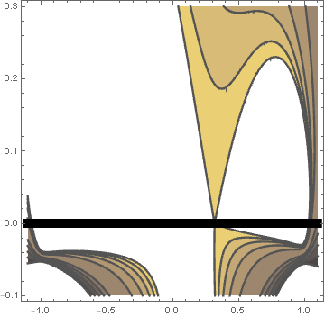
the last equality being a consequence of Eq. (3.21). Thus switching to the second integral at $z(P^{\prime})$ provides a smaller contribution than the result that would be achieved if one continues to integrate over the first integrand. This means that saddle points reached within the second integral are exponentially suppressed. Since the saddle points in the first integrals correspond to $\varphi_{+}$ or $\varphi_{-}$, respectively, the contributions related to $\varphi_{-}$ may be ignored. Fig. 1 shows the landscape on which the steepest descent curves are to be drawn.

The first integral in Eq. (3.20) is just the inverse Fourier transform of $\tilde{\varphi}$, so we obtain the following up to exponentially small terms:

$\displaystyle\int_{z(P)}^{z(P^{\prime})}e^{\imath NH(z,w)}\frac{dz}{z^{\prime}}=e^{\imath N\varphi_{+}(w)}.$

(3.26)

The reason that $\varphi_{+}(w)$ appears on the right hand side and not $\varphi_{-}(w)$ is that the saddle point reached within this integral corresponds to the analytical continuation of $H(z,w)=\varphi(z)-\varphi^{\prime}(z)(z-w)$ from the upper half plane. The saddle point reached from analytically continuing $H(z,w)$ from the lower half plane, is not reached within this integral since the relevant momentum $P(w)=\varphi_{-}^{\prime}(w)$ is too negative. Indeed, we shall show in the next paragraph that:

$\displaystyle\varphi^{\prime}_{-}(w)<P^{\prime}.$

(3.27)

To show inequation (3.27), we combine the definition of $\varphi$ with the Bethe equations, Eqs. (3.3, 2.16), repsectively, to obtain:

$\displaystyle{\rm Re}(\varphi(\theta_{i}-\imath 0^{+}))=-\frac{2\pi}{N}(n_{i}+1)$

(3.28)

where $n_{i}$ is the mode number of the Bethe root $\theta_{i}$. Taking the derivative of this equation and remembering that each mode number is represented twice, namely once for the in-state, and once more for the out-state, one obtains:

$\displaystyle{\rm Re}\varphi^{\prime}(x-\imath 0^{+})=-4\pi\rho(x),$

(3.29)

where $\rho(x)$ is the density of occupied mode numbers on the real axis. Now, as will be shown later in Eq. (3.7), in the small $c$ limit one has,

$\displaystyle\frac{1}{c}{\rm Im}\varphi(x+\imath 0^{+})=-2\pi\rho(x),$

(3.30)

so that by combining Eqs. (3.29, 3.30) and Eq. (3.21) one obtains the inequality, Eq. (3.27), given that $P$ in Eq. (3.27) is positive and in the small $c$ limit. For larger $c$ one may ascertain that the inequality holds for specific choices of $c$.

We have given above, namely in Eqs. (3.18), the solution for $\tilde{S}_{+},$ which leaves us to compute $\tilde{S}_{-}.$ In order to compute the latter, one may return to equation (3.16) and set $P$ negative, which gives the following equation for $e^{\imath N\tilde{S}_{-}}$

$\displaystyle e^{\imath N\tilde{S}_{-}(P,w)}=\int_{0}^{\infty}NdQe^{\imath N[\tilde{S}_{+}(Q,w)+\imath cQ+\tilde{\varphi}(P-Q)]}-e^{-\imath NPw}$

(3.31)

This can be further computed as follows:

		$\displaystyle e^{\imath N\tilde{S}_{-}(P,w)}=$		(3.32)
		$\displaystyle=e^{-\imath NPw}\left[e^{-\imath N\varphi_{+}(w)}\int_{z(P)}^{z(P^{\prime})}e^{\imath NH(z,w)}\frac{dz}{z^{\prime}}+e^{-NPc}\int_{P^{\prime}}^{z(-\infty)}e^{\imath NH(z,w-\imath c)}\frac{dz}{z^{\prime}}-1\right]=$
		$\displaystyle=\frac{e^{\imath N(\tilde{\varphi}(P)-\varphi_{+}(w))}}{z(P)-w}-e^{-\imath NPw}.$

The second integral on the second line is irrelevant due again to the inequality given in Eq. (3.25). The first integral receives contributions from the limits of the integration domain, but no saddle point is reached. This edge contribution gives rise to the first term in the last row of Eq. (3.32).

Taking the Fourier transform of Eq. (3.32) one obtains:

$\displaystyle R(z-\imath 0^{+},w)=\frac{e^{\imath N(\varphi(z)-\varphi_{+}(w))}-1}{z-w}.$

(3.33)

This result is of course also obtained again by the saddle point method. The saddle of integrating $e^{\imath N\tilde{\varphi}(P)+\imath Pz}$ is located of course at $z$. Depending on whether $z$ is in the upper half plane or the lower half plane, one obtains either $\varphi_{+}(z)$ or $\varphi_{-}(z)$ as a result, such that in Eq. (3.33) one may simply write $\varphi(z)$.

We can now use Eq. (3.12) to compute the Slavnov determinant. The object $R_{y}(z,w)$ is simply $R(z,w)$ after one takes $\varphi(z)\to\varphi(z)+\imath y,$ which is valid for $y<-{\rm Im}(\varphi_{+}(w)),$ while for $y>-{\rm Im}(\varphi_{+}(w)),$ the object $R_{y}(z,w)=\frac{1}{z-w}$ to exponential accuracy, but this does not contribute to the integral in Eq. (3.12) . Using then Eqs. (3.19,3.33) one obtains:

		$\displaystyle N+\log\det(\mathds{1}-K)=$		(3.34)
		$\displaystyle=N\int_{0}^{-{\rm Im}\varphi_{+}(w)}dy\int\frac{dz}{2\pi\imath}\oint\frac{dw}{2\pi\imath}\frac{e^{\imath N\left[c^{-1}(\varphi_{+}(w)+\imath y)(z-w)\right]}-e^{\imath N(\varphi(z)-\varphi_{+}(w))}}{(z-w)^{2}}.$

Performing the integral over $y$ and $z$ we obtain:

$\displaystyle N+\log\det(\mathds{1}-K)=N^{2}\int_{\chi_{\rho}}\left[\frac{\varphi_{+}^{2}(w)}{2c}-\varphi_{+}^{\prime}(w)\varphi_{+}(w)+\varphi_{+}(w)\varphi^{\prime}_{-}(w)e^{-\imath N\varphi^{J}(w)}\right]\frac{dw}{2\pi},$

(3.35)

where $\chi_{\rho}$ is the support of $\rho$. The superscript $J$ denotes the jump discontinuity of the function. Namely, for any $f$ we define $f^{J}(w)\equiv f(w+\imath 0^{+})-f(w+\imath 0^{+})$

Eq. (3.35) represents our main result for the computation of the determinants appearing in Eq. (2.22). The function $\varphi$ appearing in the expression can be computed through the thermodynamic by solving the density of roots through the thermodynamic Bethe ansatz for a given value of $c$ and then substituting this in Eq. (3.6). We believe that this result may well be extended to other Bethe ansatz models allowing the computation of Slavnov-type overlaps also there.

To obtain the small $c$ limit of the solution to the Bethe equations, first let us take the logarithm of Eq. (2.16):

$\displaystyle\imath\rho_{0}^{-1}\theta_{i}+\int\log\frac{\theta_{i}-\lambda^{\prime}-\imath c}{\theta_{i}-\lambda^{\prime}+\imath c}\rho(\lambda^{\prime})d\lambda^{\prime}=\frac{\imath\pi}{N}(2(n_{0}+i)+1),$

(4.2)

then, as usual, one takes the difference between $i+1$ and $i$ equations and multiply by

$\displaystyle\frac{-\imath j}{2\pi(\theta_{i+j}-\theta_{i})}=\frac{-\imath N\rho(\theta_{i})}{2\pi},$

(4.3)

an identity valid one assumes to be valid for $j$ small (we use it here mainly for $j=1$). This leads to:

$\displaystyle\frac{\rho_{0}^{-1}}{2\pi}+\int\left[\frac{1}{z^{\prime}-z-\imath c}-\frac{1}{z^{\prime}-z+\imath c}\right]\rho(z^{\prime})\frac{dz^{\prime}}{2\pi\imath}=\rho(z)$

(4.4)

Let us decompose of $\rho$ into function analytic in the upper and lower half planes:

$\displaystyle\rho(z)\equiv\rho_{+}(z)+\rho_{-}(z)$

(4.5)

The Bethe equations (4.4) then can be written as:

$\displaystyle\frac{1}{2\pi\rho_{0}}+\rho_{+}(z+\imath c)+\rho_{-}(z-\imath c)=\rho_{+}(\lambda)+\rho_{-}(\lambda)$

(4.6)

Which to leading order in $c$ reads:

$\displaystyle\rho^{\prime}_{+}(\lambda)-\rho^{\prime}_{-}(\lambda)=\frac{\imath\rho_{0}^{-1}}{2\pi c},$

(4.7)

which is valid on the support of $\rho$. Eqs. (4.7) and (4.5) can be solved given the condition that $\rho$ vanishes outside the support which comprises of two intervals, $[\lambda_{1},\lambda_{2}]\cup[\lambda_{3},\lambda_{4}]$. This proceudure is described now.

Consider then a function $\varphi^{(0)}(z)$ given by:

$\displaystyle\varphi^{(0)}(z)=-\rho_{0}^{-1}z-\imath 4\pi c\begin{cases}\rho^{(0)}_{+}(z)&{\rm Im}(z)>0\\ -\rho^{(0)}_{-}(z)&{\rm Im}(z)<0\\ \end{cases}.$

(4.8)

Denote by $\mathcal{S}=[\lambda_{1},\lambda_{2}]\cup[\lambda_{3},\lambda_{4}]$ the support of $\rho^{(0)}$. Then we have:

		$\displaystyle\varphi^{\prime(0)}_{+}(z)+\varphi^{\prime(0)}_{-}(z)=0,\quad z\in\mathcal{S}$		(4.9)
		$\displaystyle\varphi^{\prime(0)}_{+}(z)-\varphi^{\prime(0)}_{-}(z)=0,\quad z\notin\mathcal{S}$		(4.10)
		$\displaystyle\varphi^{\prime(0)}(z)\sim-\rho_{0}^{-1}+\frac{C}{z^{2}},\quad z\to\infty,$		(4.11)

for some $C$ (this arises from the behavior $\rho^{\prime(0)}_{\pm}(z)\to\frac{C_{\pm}}{z^{2}}$). We may solve these conditions by:

$\displaystyle\varphi^{\prime(0)}(z)=-\rho_{0}^{-1}\frac{z^{2}+a_{1}z+a_{2}}{\sqrt{R_{4}(z)}},$

(4.12)

where $R_{4}(z)=\prod_{i=1}^{4}(z-\lambda_{i}),$ and for a $a_{1}$, $a_{2}$ to be chosen below such that Eq. (4.11) is indeed satisfied.

An alternative way to solve conditions (4.9-4.11) given relation (4.8) is to write:

$\displaystyle\varphi^{(0)}(z)=2\imath c\int\frac{\rho^{(0)}(x)dx}{z-x}-\rho_{0}^{-1}z.$

(4.13)

Then one has:

$\displaystyle-2c\rho_{0}\int\frac{\rho^{(0)}(x)dx}{z-x}-z=\int_{\lambda_{1}}^{z}\frac{z^{\prime 2}+a_{1}z^{\prime}+a_{2}}{\sqrt{R_{4}(z^{\prime})}}dz^{\prime}.$

(4.14)

In order for the right hand side to be a well-defined function on the complex plane cut by the support of $\rho$, which is an obvious property of the left hand side, we must have:

$\displaystyle\int_{\lambda_{1}}^{\lambda_{2}}\frac{z^{2}+a_{1}z+a_{2}}{\sqrt{R_{4}(z)}}dz=\int_{\lambda_{3}}^{\lambda_{4}}\frac{z^{2}+a_{1}z+a_{2}}{\sqrt{R_{4}(z)}}dz=0,$

(4.15)

or in other words, that the $b$-cycles are zero. This condition fixes $a_{1}$ and $a_{2}$. In fact, the sum of both conditions is just the requirement that the pole at infinity of the integrand (considered as a differential) vanishes. This fixes $a_{1}$ to be equal to:

$\displaystyle a_{1}=-\frac{\lambda_{1}+\lambda_{2}+\lambda_{3}+\lambda_{4}}{2},$

(4.16)

while the exprtession for $a_{2}$ involves transcendental (elliptic) functions. The density is simply related to the jump discontinuity of $\varphi^{(0)}$ due to (4.8), so we have:

$\displaystyle\rho^{(0)}(z)=\int_{\lambda_{1,3}}^{z}\frac{z^{\prime 2}+a_{1}z^{\prime}+a_{2}}{\sqrt{R_{4}(z^{\prime})}}\frac{dz^{\prime}}{\imath\rho_{0}2\pi c}\quad z\in[\lambda_{1,3},\lambda_{2,4}],\mbox{ respectively}.$

(4.17)

The expressions above can be recast on the Jacobian by means of the Abel map. Namely, one has the map $z\to u(z)$ from the Riemann surface of the function $R_{4}(z)$ to the torus $\mathds{C}/\mathds{Z}\pi+\mathds{Z}\tau$. The map being given by:

$\displaystyle u(z)=\frac{1}{\omega}\int^{z}_{\lambda_{1}}\frac{dz}{R_{4}(z)},\quad\omega=\frac{2}{\pi}\int^{\lambda_{2}}_{\lambda_{1}}\frac{dz}{R_{4}(z)},$

(4.18)

and $\tau=2\frac{u(\lambda_{3})-u(\lambda_{2})}{\omega}.$

Then we have:

		$\displaystyle\varphi^{(0)}(z(u))=\frac{-1}{\rho_{0}\omega}\int^{u}_{0}(\wp(u-u_{\infty})+\wp(u+u_{\infty})+\alpha)du=$		(4.19)
		$\displaystyle=\frac{1}{\rho_{0}\omega}\left(\zeta(u+u_{\infty})+\zeta(u-u_{\infty})-\alpha u\right),$		(4.20)

where $\zeta$, $\wp$ are the weierstrass $\zeta$ and $\wp$ functions, respectively. Here $\alpha$ is determined by the condition that the $b$ cycles are zeros. Since the $b$ cycles correspond to $u\to u+\pi$, and since $\zeta(u+\pi)=\zeta(u)+2\eta$, where $\eta=\zeta\left(\frac{\pi}{2}\right)$, we have $\alpha=\frac{4\eta}{\pi},$ namely:

$\displaystyle\varphi^{(0)}(z(u))=\frac{1}{\rho_{0}\omega}\left(\zeta(u+u_{\infty})+\zeta(u-u_{\infty})-\frac{4\eta}{\pi}u\right).$

(4.21)

References

- [1] Vladimir E Korepin, Nicholay M Bogoliubov, and Anatoli G Izergin. Quantum inverse scattering method and correlation functions, volume 3. Cambridge university press, 1997.
- [2] Lorenzo Piroli and Pasquale Calabrese. Exact formulas for the form factors of local operators in the Lieb-Liniger model. Journal of Physics A Mathematical General, 48(45):454002, November 2015.
- [3] N. A. Slavnov. Calculation of scalar products of wave functions and form factors in the framework of the alcebraic Bethe ansatz. Theoretical and Mathematical Physics, 79:502–508, 1989.
- [4] E. Bettelheim and I. Kostov. Semi-classical analysis of the inner product of Bethe states. Journal of Physics A Mathematical General, 47(24):245401, 2014.
- [5] G. Gorohovsky and E. Bettelheim. Coherence factors beyond the BCS expressions – a derivation. Journal of Physics A Mathematical General, 47(2):025001, 2014.
- [6] E. Bettelheim. Towards a non-equilibrium Bethe ansatz for the Kondo model. Journal of Physics A Mathematical General, 48(16):165003, 2015.
- [7] J.-S. Caux, P. Calabrese, and N. A. Slavnov. One-particle dynamical correlations in the one-dimensional Bose gas. Journal of Statistical Mechanics: Theory and Experiment, 1:8, 2007.
- [8] Alvise Bastianello, Lorenzo Piroli, and Pasquale Calabrese. Exact Local Correlations and Full Counting Statistics for Arbitrary States of the One-Dimensional Interacting Bose Gas. Physical Review Letters, 120(19):190601, May 2018.
- [9] J. De Nardis and M. Panfil. Density form factors of the 1D Bose gas for finite entropy states. Journal of Statistical Mechanics: Theory and Experiment, 2015(2):02019, February 2015.
- [10] M. Kormos, G. Mussardo, and A. Trombettoni. Expectation Values in the Lieb-Liniger Bose Gas. Phys. Rev. Lett., 103(21):210404, November 2009.
- [11] M. Kormos, G. Mussardo, and A. Trombettoni. One-dimensional Lieb-Liniger Bose gas as nonrelativistic limit of the sinh-Gordon model. Phys. Rev. A, 81(4):043606, April 2010.
- [12] A. Koubek and G. Mussardo. On the operator content of the sinh-Gordon model. Physics Letters B, 311(1-4):193–201, July 1993.
- [13] Eugene D Belokolos. Algebro-geometric approach to nonlinear integrable equations. Springer, 1994.
- [14] Eldad Bettelheim. The Whitham approach to the limit of the Lieb-Liniger model and generalized hydrodynamics. Journal of Physics A Mathematical General, 53(20):205204, May 2020.
- [15] H. Flaschka, M. G. Forest, and D. W. McLaughlin. Multiphase averaging and the inverse spectral solution of KdV. Comm. Pure. Appl. Math., 33:739–784, 1980.
- [16] F. A. Smirnov. Quasi-classical Study of Form Factors in Finite Volume. arXiv:hep-th/9802132, 1998.
- [17] O. Babelon, D. Bernard, and F. A. Smirnov. Null-Vectors in Integrable Field Theory. Communications in Mathematical Physics, 186:601–648, 1997.
- [18] I. Kostov and Y. Matsuo. Inner products of Bethe states as partial domain wall partition functions. Journal of High Energy Physics, 10:168, 2012.
- [19] G. Gorohovsky and E. Bettelheim. Coherence Factors Beyond the BCS Result. Phys. Rev. B. Rapid Communcations, 88:060510, 2013.