Controller Synthesis for Multi-Agent Systems with Intermittent Communication and Metric Temporal Logic Specifications
Abstract
This paper investigates the controller synthesis problem for a multi-agent system (MAS) with intermittent communication. We adopt a relay-explorer scheme, where a mobile relay agent with absolute position sensors switches among a set of explorers with relative position sensors to provide intermittent state information. We model the MAS as a switched system where the explorers’ dynamics can be either fully-actuated or under-actuated. The objective of the explorers is to reach approximate consensus to a predetermined goal region. To guarantee the stability of the switched system and the approximate consensus of the explorers, we derive maximum dwell-time conditions to constrain the length of time each explorer goes without state feedback (from the relay agent). Furthermore, the relay agent needs to satisfy practical constraints such as charging its battery and staying in specific regions of interest. Both the maximum dwell-time conditions and these practical constraints can be expressed by metric temporal logic (MTL) specifications. We iteratively compute the optimal control inputs for the relay agent to satisfy the MTL specifications, while guaranteeing stability and approximate consensus of the explorers. We implement the proposed method on a case study with the CoppeliaSim robot simulator.
I Introduction
Traditionally, coordination strategies for multi-agent systems (MAS) have been designed under the assumption that state feedback is continuously available and each agent can continuously communicate with its neighbors over a network. This assumption is often impractical, especially in mobile robot applications where shadowing and fading in the wireless communication can cause unreliability, and each agent has limited energy resources [1].
Due to these constraints, there is a strong interest in developing MAS coordination methods that rely on intermittent information over a communication network. In [2, 3, 4, 5, 6, 7], the authors develop event-triggered and self-triggered controllers to only utilize sampled data from networked agents when triggered by conditions that ensure desired stability and performance properties. However, these results usually require a network represented by a strongly connected graph to enable agent coordination. In [8], the authors provided a framework where a set of explorers operating with inaccurate position sensors are able to reach consensus at a desired state while a relay agent intermittently provides each explorer with state information. By introducing a relay agent, the explorers are able to perform their tasks without the need to perform additional maneuvers to obtain state information.
Building on the work of [8, 9], we adopt a relay-explorer scheme, where the MAS is modeled as a switched system. As an illustrative example shown in Fig. 1, the three explorers need to reach approximate consensus to the green goal region and one relay agent provides intermittent state information to each explorer. To guarantee stability of the switched system and approximate consensus of the explorers, we derive maximum dwell-time conditions to constrain the intervals between consecutive time instants at which the relay agent should provide state information to the same explorer.
The maximum dwell-time conditions can be encoded by metric temporal logic (MTL) specifications [10]. Such specifications have also been used in robotic applications for time-related specifications [11]. Since the relay agent is typically more energy-consuming due to high-quality communication and mobility equipment, the relay agent is likely required to satisfy additional MTL specifications for practical constraints such as charging its battery and staying in specific regions. In the example shown in Fig. 1, the relay agent needs to satisfy an MTL specification “reach the charging station or in every 6 time units and always stay in the purple region ”.
We design the explorers’ controllers such that the guarantees on the stability of the switched system and approximate consensus of the explorers hold, provided that the maximum dwell-time conditions are satisfied. Then, we synthesize the relay agent’s controller to satisfy the MTL specifications that encode the maximum dwell-time conditions and the additional practical constraints. There is a rich literature on controller synthesis subject to temporal logic specifications [12, 13, 14, 15, 16, 17, 18]. For linear or switched linear systems, the controller synthesis problem can be converted into a mixed-integer linear programming (MILP) problem [14, 15]. Additionally, as the explorers are equipped with relative position sensors, we design an observer to estimate the explorers’ states, which can jump due to the provision of intermittent state feedback via communication. Therefore, we solve the MILP problem iteratively to account for such abrupt changes.
This paper provides additional insights and generalizes our previous work in [19]. (a) The proposed approach in [19] only applies to fully-actuated or over-actuated dynamics for the explorers, while we extend the approach to under-actuated dynamics (e.g., unicycle dynamics) for the explorers in this paper. (b) We used both maximum and minimum dwell-time conditions to achieve stability and approximate consensus for the explorers in [19], while in this paper we only rely on the maximum dwell-time conditions, i.e., the minimum dwell-time conditions are not necessary to enable the result. (c) This paper provides additional evidence of the approach through CoppeliaSim robot simulators with multiple MTL specifications in the case studies.
We implemented the proposed method on a simulation case study with three mobile robots as the explorers and one quadrotor as the relay agent. The results in two different scenarios show that the synthesized controller can lead to satisfaction of the MTL specifications, while ensuring the stability of the switched system and achieving the approximate consensus objective.

II Problem Formulation
II-A Agent Dynamics
Consider a multi-agent system (MAS) consisting of explorers () indexed by and a relay agent indexed by . Let the time set be . Let denote the position of the relay agent and explorer , respectively. Let and denote the state of the relay agent and explorer , respectively. The known linear time-invariant dynamics of the relay agent and explorer are
| (1) | ||||
where , , , and . Here, denote the control inputs of the relay agent and explorer , respectively, and denotes an exogenous disturbance that is continuous and bounded, i.e., for all ( is a known constant)11 1 denotes the 2-norm.. We assume that the pair is stabilizable.
II-B Communication
Each explorer is equipped with a relative position sensor and hardware to enable communication with other agents, e.g., the relay agent and a goal region. Since the explorers lack absolute position sensors, they are not able to localize themselves within the global coordinate system. Nevertheless, the explorers can use their relative position sensors to enable self-localization relative to their initially known locations. However, relative position sensors, like encoders and inertial measurement units (IMUs), can produce unreliable position information since wheels of mobile robots may slip and IMUs may generate noisy data. Hence, the term in (1) models the inaccurate position measurements from the relative position sensor of explorer as well as any external influences from the environment. Navigation through the use of a relative position sensor results in dead-reckoning, which becomes increasingly inaccurate with time if not corrected. On the other hand, the relay agent is equipped with an absolute position sensor and hardware to enable communication with each explorer. Unlike a relative position sensor, an absolute position sensor allows localization of the agent within the global coordinate system.
Let be a predetermined state defined by the user. A goal region (see Fig. 1) centered at the position with radius is capable of providing state information to each explorer once .
Let denote the communication radius of the relay agent and each explorer. Within this work, the relay agent has full knowledge of its own state for all and the initial state for all . The relay agent provides state information to explorer (i.e., services explorer ) if and only if and the communication channel of explorer is on. We define the communication switching signal for explorer as if the communication channel is on for explorer , and if the communication channel is off for explorer . We use to indicate the servicing instance for explorer . The servicing instance for explorer is defined as22 2 For is the initial time. For simplicity, we take
where denotes the conjunction logical connective.
II-C Approximate Consensus
Given a goal region centered at with radius , one objective is to design distributed controllers for all explorers that achieve approximate consensus within the goal region. This objective is decomposed into two tasks, where it is the task of the explorers to dead-reckon towards , and it is the task of the relay agent to intermittently service each explorer.
Since a single relay agent must intermittently service explorers, the MAS can be modeled as a switched system, where the relay agent has modes of operation, i.e., the relay agent can service no, a single, multiple, or all explorers at an instance depending on the configuration of the explorers. Let be a piece-wise constant switching signal that determines the mode of operation for the relay agent, where denotes the power set of . The switching signal also determines the servicing times for all explorers, i.e., . To quantify the objective, let the tracking error of explorer be defined as
| (2) |
To facilitate the analysis, let the state estimation error be defined as
| (3) |
where denotes the state estimate of explorer . For each , the state estimate of explorer is synchronized between explorer and the relay agent. Let the estimated tracking error be defined as
| (4) |
Using (3) and (4), (2) can be alternatively expressed as
| (5) |
Given the tracking error in (2), approximate consensus is achieved within the goal region whenever
where denotes the maximum singular value of .
II-D State Observer and Controller Development
The state estimate of explorer is generated by the following model-based observer
| (6) | ||||
where the position estimate of explorer is defined as
| (7) | ||||
The state estimate is initialized as for all . Note that at each servicing instance , the state estimate of explorer is reset to as outlined in (6). The controller of explorer is defined as
| (8) |
where is the positive definite solution to the Algebraic Riccati Equation (ARE) given by
| (9) |
such that is a user-defined parameter, denotes the identity matrix, and denotes the zero matrix. Substituting (1) and (6) into the time derivative of (3) yields
| (10) | ||||
where denotes the -dimensional zero vector. Substituting (6) and (8) into the time derivative of (4) yields
| (11) | ||||
Substituting (1), (5), and (8) into the time derivative of (2) yields
| (12) | ||||
The state is continuous given the motion model in (1). Hence, (2) implies is continuous. From (3) and (6), is piece-wise continuous. Since the disturbance acting on explorer is continuous, is continuous, and is piece-wise continuous, the RHS of (12) is piece-wise continuous. Hence, is piece-wise continuously differentiable, and therefore, locally Lipschitz.
II-E Metric Temporal Logic (MTL)
To achieve stability of the switched system and approximate consensus of the explorers while satisfying the practical constraints of the relay agent, the requirements of the MAS can be specified in MTL specifications (see details in Section IV). In this subsection, we briefly review MTL interpreted over discrete-time trajectories [20]. The domain of the position of a certain agent is denoted by . The Boolean domain is , and the time index set is . With slight abuse of notation, we use to denote the discrete-time trajectory as a function from to . A set is a set of atomic propositions, each of which maps to . The syntax of MTL is defined recursively as
where stands for the Boolean constant True, is an atomic proposition, (negation), (conjunction), (disjunction) are standard Boolean connectives, is a temporal operator representing “until” and is a time interval of the form (, ). We can also derive two useful temporal operators from “until” (), which are “eventually” and “always” . We define the set of states that satisfy the atomic proposition as .
Next, we introduce the Boolean semantics of MTL for trajectories of finite length in the strong and the weak view, which are modified from the literature of temporal logic model checking and monitoring [21, 22, 23]. We use to denote the time instant at time index and to denote the value of at time . In the following, (resp. ) means the trajectory strongly (resp. weakly) satisfies at time index , (resp. ) means fails to strongly (resp. weakly) satisfy at time index .
Definition 1.
The Boolean semantics of MTL for trajectories of finite length in the strong view is defined recursively as follows [16]:
Definition 2.
The Boolean semantics of MTL for trajectories of finite length in the weak view is defined recursively as follows [16]:
Intuitively, if a trajectory of finite length can be extended to infinite length, then the strong view indicates that the truth value of the formula on the infinite-length trajectory is already “determined” on the trajectory of finite length, while the weak view indicates that it may not be “determined” yet [23]. As an example, a trajectory is not possible to strongly satisfy at time 0, but is possible to strongly violate at time 0, i.e., is possible.
For an MTL formula , the necessary length is defined recursively as follows [24]:
II-F Problem Statement
We now present the problem formulation for the control of the MAS with intermittent communication and MTL specifications.
Problem 1.
Design the control inputs for the relay agent ( denotes the control input at time index ) such that the following characteristics are satisfied while minimizing the control effort :
Correctness: A given MTL specification is weakly satisfied by the trajectory of the relay agent.
Stability: The error signal is uniformly bounded for each .
Approximate Consensus: The states of the explorers reach approximate consensus within the goal region centered at with radius .
III Stability and Consensus Analysis
In this section, we provide conditions that generate a stable switched system and enable approximate consensus for the explorers.
To facilitate the stability analysis, we define the following objects. Let and denote the maximum and minimum eigenvalue of the symmetric matrix , respectively. Let , where is a bounding constant such that . Recall that is an upper bound for the disturbance acting of explorer . Let be an essentially bounded measurable function. Then, if and only if . Let be a user-defined parameter that quantifies the maximum tolerable state estimation error, i.e., it is desirable to ensure for all and . We now derive a maximum dwell-time condition that ensures for all , where continuous satisfaction of the maximum dwell-time condition by the relay agent ensures for all .
Theorem 1.
If and the relay agent satisfies the maximum dwell-time condition given by
| (13) |
then for all .
Proof.
Let , and suppose .33 3 because the relay agent serviced explorer at time . Consider the common Lyapunov-like functional candidate defined as . Given (1) and (6), (3) is continuously differentiable over Substituting (10) into the time derivative of yields which can be upper bounded by
| (14) |
Using the definition of , (14) can be upper bounded by . Using the Comparison Lemma [25, Lemma 3.4] over ,
| (15) |
Substituting the definition of into (15) yields . Define as
| (16) |
Since for all and , where and we see that for all If then for all Moreover, yields the dwell-time condition in (13). Hence, for all provided and (13) hold. ∎
Next, we show that the observer in (6) ensures the estimated tracking error in (4) is exponentially regulated for all and each servicing instance .
Theorem 2.
Proof.
Consider the common Lyapunov functional defined as . By the Rayleigh quotient, it follows that
| (18) |
By (6), (4) is continuously differentiable over . Substituting (11) into the time derivative of yields
| (19) |
Using the ARE in (9), it follows that (19) is equivalent to . Using (18), we then see that
| (20) |
Invoking the Comparison Lemma in [25, Lemma 3.4] on (20) over yields
| (21) |
where substituting the definition of and (18) into (21) yields (17). ∎
We now show the tracking error in (2) is uniformly ultimately bounded (UUB).
Theorem 3.
Proof.
Suppose the relay agent satisfies the maximum dwell-time condition in (13) for each and . Consider the common Lyapunov functional defined by . Recall that is continuous, and is piece-wise continuous, where the discontinuities occur at each servicing instance. Hence, the set of discontinuities is countable. By the Rayleigh quotient, it follows that
| (23) |
Substituting (12) into the time derivative of yields
| (24) | ||||
Using the ARE in (9), it follows that (24) can be upper bounded as
| (25) | ||||
Since the relay agent satisfies the maximum dwell-time condition in (13) for each , for all by Theorem 1. Recall that and that . Hence, (25) can be upper bounded as
| (26) |
where the auxiliary constant is defined in Theorem 3. Substituting (23) into (26) and integrating both sides of the resulting inequality over yields (22). Observe that (22) implies . Since and given the relay agent satisfies the maximum dwell-time condition in (13) for each , (5) implies . Hence, given (8) and . ∎
Remark 1.
From (22), we see that
where can be made small by making small, i.e., selecting a small and setting the desired state as the origin. A change of coordinate transformation can be used to make the desired state the origin.
Remark 2.
Note that . If the radius of the goal region is selected such that , then provided . Since within the goal region, can be reduced to , where .
IV Controller Synthesis with Intermittent Communication and MTL Specifications
In this section, we provide the framework and algorithms for controller synthesis of the relay agent to satisfy the maximum dwell-time conditions and the practical constraints. The controller synthesis for the relay agent is conducted iteratively as the state estimates for the explorers are reset to the true state values whenever they are serviced by the relay agent, and thus the control inputs need to be recomputed with the reset values.
We define the discrete time set , where for , and is the sampling period. The maximum dwell-time in (13) for explorer is in the interval for some non-negative integer . We use the following MTL specifications for encoding the maximum dwell-time condition ( is a user-defined parameter):
| (27) | ||||
where means “for any explorer , the relay agent needs to be within distance from the estimated position of explorer at least once in any time periods”.
The relay agent also needs to satisfy an MTL specification for the practical constraints. One example of is as follows.
| (28) |
which means “the relay agent needs to reach the charging station or at least once in any time periods, and it should always remain in the region ” ( is a positive integer).
Combining and , the MTL specification for the relay agent is . We use to denote the formula modified from the MTL formula when is evaluated at time index and the current time index is . can be calculated recursively as follows (we use to denote the atomic predicate evaluated at time index ):
| (29) | ||||
where stands for the Boolean constant False. If the MTL formula is evaluated at the initial time index (which is the usual case when the task starts at the initial time), then the modified formula is .
Algorithm 1 shows the controller synthesis approach with intermittent communication and MTL specifications. The controller synthesis problem can be formulated as a sequence of mixed integer linear programming (MILP) problems, denoted as MILP-sol in Line 3, and expressed as follows:
| (30) |
| subject to: | ||||
| (31) | ||||
| (32) | ||||
| (33) | ||||
| (34) |
where the time index is initially set as 0, is the number of time instants in the control horizon, , is the control inputs of the relay agent, the input values are constrained to , , , , , and are converted from , , , , and respectively for the discrete-time state-space representation, and are control inputs of explorer from (8). Note that we only require the trajectory to weakly satisfy as may be less than the necessary length .
At each time index , we check if there exists any explorer that is being serviced (Line 5). If there are such explorers, we update the state estimates of those explorers with their true state values (Line 7). Then, we modify the MTL formula as in (29). The MILP is solved for time index with the updated state values and the modified MTL formula (Line 8). The previously computed relay agent control inputs are replaced by the newly computed control inputs from time index to (Line 9).
We use to denote the time that holds in the discrete time set for explorer 44 4 For is the initial time, i.e., , i.e.,
We design the communication switching signal as follows:
| (35) |
Finally, we present Theorem 4, which provides theoretical guarantees for achieving correctness, stability and approximate consensus (in Problem 1).
Theorem 4.
With the observers in (6), the controllers for the explorers in (8), communication switching signal in (35), if each optimization is feasible in Algorithm 1, , , and , then Algorithm 1 terminates within finite time, the MTL specification is weakly satisfied and the explorers reach approximate consensus within the goal region in the sense that , where .
Proof.
We first use induction to prove that for each and . For each , if , then . Now fix and assume that for some . We now show that . If each optimization is feasible in Algorithm 1, then . Then, following the analysis in the proof of Theorem 1, . Thus, we have . Therefore, if , then . According to the communication switching signals in (35), . Thus, from the definition of in Section II-B, holds. Therefore, for each and by mathematical induction.
If each optimization is feasible in Algorithm 1, then the MTL specification is weakly satisfied. With , the maximum dwell-time condition in (13) is satisfied for all and . From Theorem 3 and Remarks 1 and 2, if holds, then, for each , there exists a time such that explorer will be inside the goal region for . Thus, at time , holds for any , i.e., Algorithm 1 is guaranteed to terminate within finite time. Finally, if , then according to Theorem 3 and Remark 2, we have . ∎
V Implementation
We now demonstrate the controller synthesis approach on the example in Fig. 1 (in Section I). The relay agent is a quadrotor modeled as a 3-D six degrees of freedom (6-DOF) rigid body [16]. We denote the system state as , where and are the position and velocity vectors of the quadrotor. The vector includes the roll, pitch and yaw Euler angles of the quadrotor. The vector includes the angular velocities rotating around its body frame axes. The general nonlinear dynamic model of such a quadrotor is given by
| (36) | ||||
where is the mass, is the gravitational acceleration, is the inertia matrix, is the rotation matrix representing the body frame with respect to the inertia frame (which is a function of the Euler angles), is the nonlinear mapping matrix that projects the angular velocity to the Euler angle rate , , is the thrust of the quadrotor, and is the torque on the three axes. The control input is , where is the vertical velocity command, and are the angular velocity commands around its three body axes. By adopting the small-angle assumption and then linearizing the dynamic model around the hover state, a linear kinematic model can be obtained as
| (37) |
where is the state of the kinematic model of the quadrotor (relay agent), , and . For the 3-D position representation, .
The dynamics of the differential drive of explorer can be feedback linearized into the following equations (see Section V of [16]):
| (38) |
where and are the inputs in the 2-D plane.
For the state space representation, , , and . The initial 3-D positions of the three explorers are , and , respectively. The vertical positions of the explorers are all zero. The initial 3-D position of the relay agent is . The consensus state is set as . The random disturbance is a vector whose elements are drawn at each time step from a standard uniform distribution centered about the origin spanning for all , where , and .
For approximate consensus, we consider the controller of the explorers in (8), where is as follows (computed from (9) with ).
| (39) |
We consider two different scenarios as follows.
| MTL specification |
| ||
|---|---|---|---|
|
|
70,943.32 | ||
|
|
101,079.03 | ||
|
|
165,224.55 |
| MTL specification |
| ||
|---|---|---|---|
|
|
644,670.20 | ||
|
|
165,984.72 | ||
|
|
165,241.50 |
Scenario 1: We consider three MTL specifications for as shown in Table I. The relay agent needs to reach the charging station or at least once in any time, and it should always remain in region , where the two charging stations and are rectangular cuboids with length, width and height being 10, 10 and 5, centered at and , respectively. The region is a rectangular cuboid centered at with length, width and height being 300, 300 and 6, respectively (see Fig. 1).
Scenario 2: We consider three MTL specifications for as shown in Table II. The relay agent needs to reach the charging station or at least once in any time, always remain in region (same as in Scenario 1), and never stay in region for over time, where the region is a rectangular cuboid centered at with length, width and height being 75, 75 and 4, respectively.
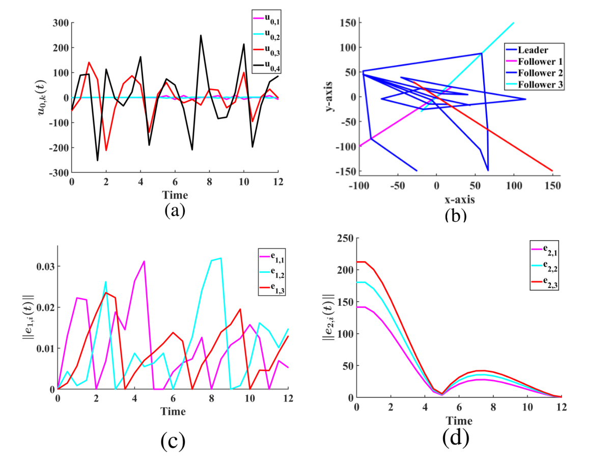
We set , , , and . Fig. 2 shows the simulation results in Scenario 1. We observe that the obtained control inputs of the relay agent gradually decrease as the explorers approach the goal region, is uniformly bounded by , and gradually decreases and then oscillates when the explorers approach approximate consensus to the goal region. We measure the cumulative control effort as , where denotes the minimal time index such that for all . The results as shown in Table I also show that the cumulative control effort for satisfying is more than that for satisfying , which is still more than that for satisfying . This is consistent with the fact that implies , and implies both and .
Fig. 3 shows the simulation results in Scenario 2. We observe that is uniformly bounded by and gradually decreases and then oscillates when the explorers approach approximate consensus to the goal region. The results as shown in Table II also show that the cumulative control effort for satisfying is more than that for satisfying , which is still more than that for satisfying . This is consistent with the fact that implies , and implies both and . We also observe that more cumulative control effort is needed in Scenario 2 to satisfy the MTL specifications after the explorers arrive in region as the relay agent needs to get away from after each service to the explorers. Videos of the simulations in both scenarios are available in the CoppeliaSim environment55 5 CoppeliaSim videos can be found at https://tinyurl.com/y32xgmtx..

VI Conclusion
We present a metric temporal logic approach for the controller synthesis of a multi-agent system with intermittent communication. We iteratively solve a sequence of mixed-interger linear programming problems for provably achieving correctness, stability of the switched system and approximate consensus of the explorers. Since the explorers are specified to reach approximate consensus in this paper, we will investigate scenarios where controller synthesis can be also conducted for the explorers with more complex specifications.
References
- [1] A. Goldsmith, Wireless communications. Cambridge university press, 2005.
- [2] X. Wang and M. Lemmon, “Self-triggered feedback control systems with finite-gain stability,” IEEE Trans. Autom. Control, vol. 54, pp. 452–467, Mar. 2009.
- [3] X. Meng and T. Chen, “Event based agreement protocols for multi-agent networks,” Automatica, vol. 49, pp. 2125–2132, Jul. 2013.
- [4] T. H. Cheng, Z. Kan, J. R. Klotz, J. M. Shea, and W. E. Dixon, “Event-triggered control of multi-agent systems for fixed and time-varying network topologies,” IEEE Trans. Autom. Control, vol. 62, no. 10, pp. 5365–5371, 2017.
- [5] H. Li, X. Liao, T. Huang, and W. Zhu, “Event-triggering sampling based leader-following consensus in second-order multi-agent systems,” IEEE Trans. Autom. Control, vol. 60, no. 7, pp. 1998–2003, Jul. 2015.
- [6] W. Heemels and M. Donkers, “Model-based periodic event-triggered control for linear systems,” Automatica, vol. 49, no. 3, pp. 698–711, 2013.
- [7] P. Tabuada, “Event-triggered real-time scheduling of stabilizing control tasks,” IEEE Trans. Autom. Control, vol. 52, no. 9, pp. 1680–1685, 2007.
- [8] F. Zegers, H.-Y. Chen, P. Deptula, and W. E. Dixon, “A switched systems approach to consensus of a distributed multi-agent system with intermittent communication,” in Proc. IEEE Amer. Control Conf., 2019.
- [9] H. Chen, Z. I. Bell, P. Deptula, and W. E. Dixon, “A switched systems approach to path following with intermittent state feedback,” IEEE Transactions on Robotics, vol. 35, no. 3, pp. 725–733, June 2019.
- [10] J. Ouaknine and J. Worrell, “On the decidability of metric temporal logic,” in Proc. Annual IEEE Symposium on Logic in Computer Science, ser. LICS’05. Washington, DC, USA: IEEE Computer Society, 2005, pp. 188–197. [Online]. Available: https://doi.org/10.1109/LICS.2005.33
- [11] Z. Xu and U. Topcu, “Transfer of temporal logic formulas in reinforcement learning,” in IJCAI-19. International Joint Conferences on Artificial Intelligence Organization, 7 2019, pp. 4010–4018.
- [12] H. Kress-Gazit, G. Fainekos, and G. Pappas, “Temporal-logic-based reactive mission and motion planning,” IEEE Trans. Robot., vol. 25, no. 6, pp. 1370–1381, Dec. 2009.
- [13] T. Wongpiromsarn, U. Topcu, and R. M. Murray, “Receding horizon temporal logic planning,” IEEE Trans. Autom. Control, vol. 57, no. 11, pp. 2817–2830, Nov 2012.
- [14] A. Donzé and V. Raman, “BluSTL: Controller synthesis from signal temporal logic specifications,” in Proc. 1st and 2nd Int. Workshop Applied Verification for Continuous and Hybrid Syst., G. Frehse and M. Althoff, Eds., vol. 34. EasyChair, 2015, pp. 160–168.
- [15] S. Saha and A. A. Julius, “An MILP approach for real-time optimal controller synthesis with metric temporal logic specifications,” in Proc. IEEE Amer. Control Conf., July 2016, pp. 1105–1110.
- [16] Z. Xu, S. Saha, B. Hu, S. Mishra, and A. A. Julius, “Advisory temporal logic inference and controller design for semiautonomous robots,” IEEE Trans. Autom. Sci. Eng., pp. 1–19, 2018.
- [17] Z. Xu, A. Julius, and J. H. Chow, “Energy storage controller synthesis for power systems with temporal logic specifications,” IEEE Systems Journal, vol. 13, no. 1, pp. 748–759, 2019.
- [18] Z. Liu, B. Wu, J. Dai, and H. Lin, “Distributed communication-aware motion planning for networked mobile robots under formal specifications,” IEEE Trans. Control. Netw. Syst., 2020.
- [19] Z. Xu, F. M. Zegers, B. Wu, W. E. Dixon, and U. Topcu, “Controller synthesis for multi-agent systems with intermittent communication: A metric temporal logic approach,” 57th Annual Allerton Conference on Communication, Control, and Computing, pp. 1015–1022, 2019.
- [20] G. E. Fainekos and G. J. Pappas, “Robustness of temporal logic specifications,” in Formal Approaches to Testing and Runtime Verification, in: LNCS, vol. 4262, Springer, 2006.
- [21] C. Eisner, D. Fisman, J. Havlicek, Y. Lustig, A. McIsaac, and D. Van Campenhout, Reasoning with Temporal Logic on Truncated Paths. Berlin, Heidelberg: Springer Berlin Heidelberg, 2003, pp. 27–39.
- [22] O. Kupferman and M. Y. Vardi, “Model checking of safety properties,” Form. Methods Syst. Des., vol. 19, no. 3, pp. 291–314, Oct. 2001. [Online]. Available: https://doi.org/10.1023/A:1011254632723
- [23] H.-M. Ho, J. Ouaknine, and J. Worrell, “Online monitoring of metric temporal logic,” in Proc. Int. Conf. Runtime Verification, B. Bonakdarpour and S. A. Smolka, Eds. Cham: Springer Int. Publishing, 2014, pp. 178–192.
- [24] O. Maler and D. Nickovic, Monitoring Temporal Properties of Continuous Signals. Berlin, Heidelberg: Springer Berlin Heidelberg, 2004, pp. 152–166. [Online]. Available: http://dx.doi.org/10.1007/978-3-540-30206-3_12
- [25] H. K. Khalil, Nonlinear Systems, 3rd ed. Upper Saddle River, NJ, USA: Prentice Hall, 1996.