∎
An Empirical Study of Graph-Based Approaches for Semi-Supervised Time Series Classification
Abstract
Time series data play an important role in many applications and their analysis reveals crucial information for understanding the underlying processes. Among the many time series learning tasks of great importance, we here focus on semi-supervised learning based on a graph representation of the data. Two main aspects are involved in this task. A suitable distance measure to evaluate the similarities between time series, and a learning method to make predictions based on these distances. However, the relationship between the two aspects has never been studied systematically in the context of graph-based learning. We describe four different distance measures, including (Soft) DTW and MPDist, a distance measure based on the Matrix Profile, as well as four successful semi-supervised learning methods, including the graph Allen–Cahn method and a Graph Convolutional Neural Network. We then compare the performance of the algorithms on binary classification data sets. In our findings we compare the chosen graph-based methods using all distance measures and observe that the results vary strongly with respect to the accuracy. As predicted by the “no free lunch” theorem, no clear best combination to employ in all cases is found. Our study provides a reproducible framework for future work in the direction of semi-supervised learning for time series with a focus on graph representations.
Keywords:
Semi-supervised learning time series graph Laplacian Allen–Cahn equation graph convolutions network1 Introduction
Data are available more abundant than ever before and many of the observed processes produce data that are time-dependent. As a result the study of time series data is a subject of great importance Fu 2011; Bello-Orgaz et al. 2016; Chen et al. 2015 and many different tasks are of interest depending on the particular application. The case of time series is interesting for tasks such as anomaly detection Laptev et al. 2015, motif computation Chiu et al. 2003 or time series forecasting De & Hyndman 2006. We refer to Wei 2006; Chatfield & Xing 2019; Fawaz et al. 2019; Abanda et al. 2019 for more general introductions.
We here focus on the task of classification of time series Wei & Keogh 2006; Liao 2005; Aghabozorgi et al. 2015 in the context of semi-supervised learning Zhu & Goldberg 2009; Chapelle et al. 2009 where we want to label all data points based on the fact that only a small portion of the data is already pre-labeled.
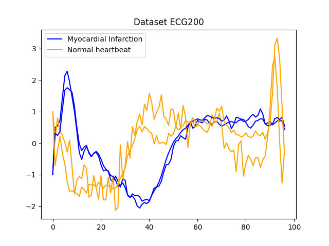
An example is given in Fig. 1 where we see some time series reflecting ECG data and the classification into normal heartbeats on the one hand and myocardial infarction on the other hand. In our applications, we assume that only for some of the time series the corresponding class is known a priori. Our focus is on the case when the data are incorporated into a graph. Each time series becomes a node within a weighted undirected graph and the edge-weight is proportional to the similarity between different time series. Graph-based approaches have become a standard tool in many learning tasks (cf. Stoll 2020; Mercado et al. 2019; Kipf & Welling 2016; Bertozzi et al. 2018; Luxburg 2007; Bruna et al. 2013 and the references mentioned therein). The matrix representation of the graph via its Laplacian Chung & Graham 1997 leads to studying the network using matrix properties. An important ingredient in the construction of the Laplacian is the choice of the appropriate weight function. In many applications, the computation of the distance between time series or sub-sequences becomes a crucial task and this will be reflected in our choice of weight function. We consider several distance measures such as DTW Müller 2007, soft DTW Cuturi & Blondel 2017, and matrix profile Gharghabi et al. 2020.
We will embed these measures via the graph Laplacian into two different recently proposed semi-supervised learning frameworks. Namely, a diffuse interface approach that originates from material science Bertozzi & Flenner 2012 via the graph Allen-Cahn equation as well as a method based on graph convolutional networks Kipf & Welling 2016. Since these methods have originally been introduced outside of the field of time series learning, their relationship with time series distance measures has never been studied. Our goal is furthermore to compare these approaches with the well-known 1NN approach Wei & Keogh 2006 and a simple optimization formulation solved relying on a linear system of equations. Our motivation follows that of Bagnall et al. 2017, where many methods for supervised learning in the context of time series were compared, namely that we aim to provide a wide-ranging overview of recent methods based on a graph representation of the data and combined with several distance measures.
We structure the paper as follows. In Section 2 we introduce some basic notations and make the case for transforming the data to graph form based on a motivation from unsupervised learning. In Section 3 we discuss several distance measures with a focus on the well-known DTW measure as well as two recently emerged alternatives, i.e. Soft DTW and the MP distance. We use Section 4 to introduce the two semi-supervised learning methods in more detail, followed by a shorter description of their well-known competitors. Section 5 will allow us to compare the methods and study the hyperparameter selection.
2 Basics
We consider discrete time series given as a vector of real numbers of length . In general, we allow for the time series to be of different dimensionality; later we often consider all . We assume that we are given time series . The goal of a classification task is to group the time series into a number of different clusters with . In this paper we focus on the task of semi-supervised learning Zhu & Goldberg 2009 where only some of the data are already labeled but we want to classify all available data simultaneously. Nevertheless, we review some techniques for unsupervised learning first as they deliver useful terminology. As such the k-means algorithm is a prototype-based clustering algorithm that divides the given data into a predefined number of clusters MacQueen 1967. The idea behind -means is rather simple as the cluster centroids are repeatedly updated and the data points are assigned to the nearest centroid until the centroids and data points have converged. Often the termination condition is not handled that strictly. For example, the method can be terminated when only 1% of the points change clusters. The starting classes are often chosen at random but can also be assigned in a more systematic way by calculating the centers first and then assign the points to the nearest center. While -means remains very popular it also has certain weaknesses coming from its minimization of the sum of squared errors loss function MacKay & Mac 2003. We discuss this method in some detail here to point out the main mechanism and this is the measuring of all distances in the Euclidean norm, which would also be done when -means is applied to time series. A simple two-dimensional example is shown in Fig. 2 where it is clear to see that -means fails to capture the data manifold. In comparison, the alternative method shown, i.e., a spectral clustering technique, performs much better. We briefly discuss this method next as it forms the basis of the main techniques introduced in this paper.


2.1 Graph Laplacian and spectral clustering
As we illustrated in Fig. 2 the separation of the data into two-classes is rather difficult for -means as the centroids are based on a -norm minimization. One alternative to -means is based on interpreting the data points as nodes in a graph. For this, we assume that we are given data points and some measure of similarity Luxburg 2007. We define the weighted undirected similarity graph with the vertex or node set and the edge set . We view the data points as vertices, , and if two nodes have a positive similarity function value, they are connected by an edge with weight equal to that similarity. With this reformulation of the data we turn the clustering problem into a graph partitioning problem where we want to cut the graph into two or possibly more classes. This is usually done in such a way that the weight of the edges across the partition is minimal.
We collect all edge weights in the adjacency matrix . The degree of a vertex is defined as and the degree matrix is the diagonal matrix holding all node degrees. In our case we use a fully connected graph with the Gaussian similarity function
| (1) |
where is a scaling parameter and is a particular distance function, such as the Euclidean distance . Note that for similar nodes, the distance function is small while the similarity function is relatively large.
We now use both the degree and weight matrix to define the graph Laplacian as . Often the symmetrically normalized Laplacian defined via
| (2) |
provides better clustering information Luxburg 2007. It has some very useful properties that we will exploit here. For example, given a non-zero vector we obtain the energy term
| (3) |
Using this it is easy to see that is positive semi-definite with non-negative eigenvalues . The main advantage of the graph Laplacian is that based on its spectral information one can usually rely on transforming the data into a space where they are easier to separate Chung & Graham 1997; Luxburg 2007; Belkin & Niyogi 2001. As a result one typically requires the spectral information corresponding to the smallest eigenvalues of The most famed eigenvector is the Fiedler vector, i.e., the eigenvector corresponding to the first non-zero eigenvalue, which is bound to have a sign change and as a result can be used for binary classification. The weight function (1) is also found in kernel methods Shawe-Taylor & Cristianini 2004; Hofmann et al. 2008 when the radial basis kernel is applied.
2.2 Self-tuning
In order to improve the performance of the methods based on the graph Laplacian, tuning the parameter is crucial. While hyperparameter tuning based on a grid search or cross validation is certainly possible we also consider a that adapts to the given data. For spectral clustering, such a procedure was introduced in Zelnik-Manor & Perona 2005. Here we use this technique to learning with time series data. For each time series we assume a local scaling parameter . As a result, we have the generalized square distance as
| (4) |
and this gives the following adjacency matrix
| (5) |
The authors in Zelnik-Manor & Perona 2005 choose as the distance to the -th nearest neighbor of where is a fixed parameter, e.g., is used in Bertozzi & Flenner 2012.
In Section 5 we will explore several different values for and their influence on the classification behavior.
3 Distance measures
We have seen so far that the Laplacian as well as typical kernel methods will rely on the choice of the distance measure . If all time series are of the same length then the easiest distance measure would be a Euclidean distance, which especially for large is fast to compute. This makes the Euclidean distance incredibly popular but it suffers from being sensitive to small shifts in the time series. As a result we discuss several popular and efficient methods for different distance measures. Our focus is to illustrate in an empirical study how the choice of distance measure impacts the performance of graph-based learning and it is clear that very likely there will be no clear winner in this competition but rather further insights for future research (cf. Keogh & Kasetty 2003).
3.1 Dynamic Time Warping
We first discuss the distance measure of Dynamic Time Warping (DTW, Müller 2007). By construction, DTW is an algorithm to find an optimal alignment between time series.
In the following, we adapt the notation of Müller 2007 to our case. Consider two time series and of lengths and , respectively, with entries for and . We obtain the local cost matrix by assembling the local differences for each pair of elements, i.e., .
The DTW distance is defined via -warping paths, which are sequences of index tuples with boundary, monotonicity, and step size conditions
The total cost of such a path with respect to is defined as
The DTW distance is then defined as the minimum cost of any warping path:
| (6) |
Both the warping and the warping path are illustrated in Fig. 3.


Computing the optimal warping path directly quickly becomes infeasible. However, we can use dynamic programming to evaluate the accumulated cost matrix recursively via
| (7) |
The actual DTW distance is finally obtained as
| (8) |
The DTW method is a heavily used distance measure for capturing the sometimes subtle similarities between time series. In the literature it is often stated that the computational cost of DTW are often described as too high. As a result one is interested in accelerating the DTW algorithm itself. One possibility arises from imposing additional constraints (cf. Müller 2007; Salvador & Chan 2004) such as the Sakoe-Chiba Band and the Itakura parallelogram. While these are appealing concepts the authors in Wu & Keogh 2020 observe that the well-known FastDTW algorithm is in fact slower than DTW. As such, we rely on the implementation of DTW provided via https://github.com/wannesm/dtaidistance. We observe that for this implementation of DTW indeed FastDTW is outperformed frequently.
3.2 Soft Dynamic Time Warping
Based on a slight reformulation of the above DTW scheme, we want to look at another time series distance measure, the Soft Dynamic Time Warping (Soft DTW). It is an extension of DTW designed to allow differentiable introduced in Blondel et al. 2020; Cuturi & Blondel 2017. We again start from the cost matrix with for time series and . Each warping path can equivalently be described by a matrix with the following condition: The ones in form a path starting in going to , only using steps downwards, to the right and diagonal downwards. is called monotonic alignment matrix and we denote the set containing all these alignment matrices with . The Frobenius inner product is then the sum of costs along the alignment . Solving the following minimization problem leads us to a reformulation of the dynamic time warping introduced above as
| (9) |
With Soft DTW we involve all alignments possible in by replacing the minimization with a soft minimum:
| (10) |
This function approximates the minimum of and is differentiable. The parameter controls the tuning between smoothness and approximation of the minimum. Using the DTW-function (9) within (10) yields the expression for Soft Dynamic Time Warping written as
| (11) |
This is now a differentiable alternative to DTW, which involves all alignments in our cost matrix.
Due to entropic bias, Soft DTW can generate negative values, which would cause issues for our use in time series classification. We apply the following remedy to overcome this drawback:
| (12) |
This measure is called Soft DTW divergence Blondel et al. 2020 and will be employed in our experiments.
3.3 Matrix Profile Distance
Another alternative time series measure that has recently been introduced is the Matrix Profile Distance (MP distance, Gharghabi et al. 2020). This measure is designed for fast computation and finding similarities between time series.
We will again introduce the concept of the matrix profile of two time series and . The matrix profile is based on the subsequences of these two time series. For a fixed window length , the subsequence of a time series is defined as a contiguous -element subset of via . The all-subsequences set of contains all possible subsequences of with length , , where is again the length of .
For the matrix profile, we need the all-subsequences sets and of both time series and . The matrix profile is the set consisting of the closest Euclidean distances from each subsequence in to any subsequence in and vice versa:
With the matrix profile, we can finally define the MP distance based on the idea that two time series are similar if they have many similar subsequences. We do not consider the smallest or the largest value of because then the MP distance could be too rough or too detailed. For example, if we would have two rather similar time series, but either one has a noisy spike or some missing values, then the largest value of the matrix profile could give a wrong impression about the similarity of these two time series. Instead, the distance is defined as
where the parameter is typically set to of Gharghabi et al. 2020.
We now illustrate the MP distance using an example as illustrated in Fig. 4(a), where we display three time series of length Our goal is to compare these time series using the MP distance. We observe that and have quite similar oscillations. The third time series does not share any obvious features with the first two sequences.


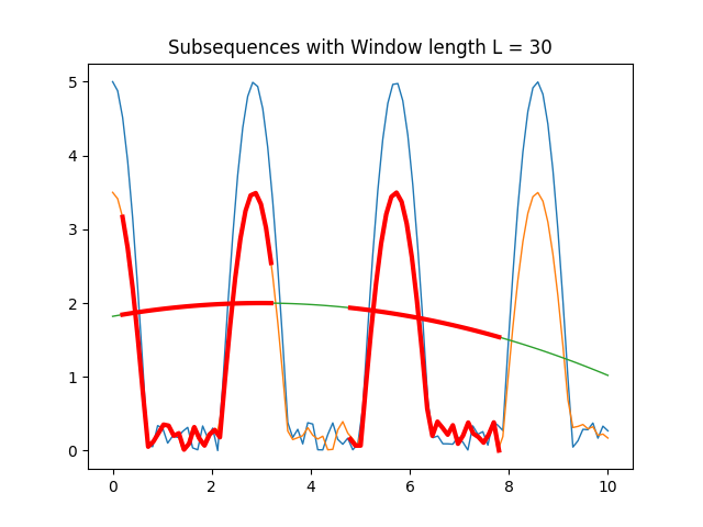
The MP distance compares the subsequences of the time series, depending on the window length . Choosing the window length to be , we get the following distances:
As we can see, the MP distance identified the similarity between and show the difference between the series and . We also want to show that the MP Distance depends on the window length . Let us look at the MP distance between the lower oscillation time series and , which is varying a lot for different values of as indicated in Table 1. Choosing there is not a large portion of both time series to compare with and as a result we observe a small value for the MP distance, which does not describe the dissimilarity of and in a proper way. If we look at , there is a larger part of the time series structure to compare the two series. If there is a special recurring pattern in the time series, the length should be large enough to cover one recurrence. We illustrate the comparison based on different window lengths in Fig. 4(b) and 4(c).
| L | 10 | 20 | 30 | 40 |
|---|---|---|---|---|
| 0.270 | 2,034 | 3,955 | 5,404 |
For the tests all data sets consist of time series with a certain length, varying for each data set. Thus we have to decide which window length should be chosen automatically in the classifier. An empirical study showed that choosing gives good classification results.
We briefly illustrate the computing times of the different distance measures when applied to time series of increasing length shown in Fig. 5. It can be seen that DTW is faster than fastDTW. Obviously, the Euclidean distance shows the best scalability. We also observe that the computation of the SDTW is scaling worse than the competing approaches when applied to longer time series.
4 Semi-supervised learning based on graph Laplacians
In this section we propose the use of two methods that have recently gained wide attention. This first method is inspired by a partial differential equation model originating from material science and the second approach is based on neural networks that incorporate the graph structure of the labeled and unlabeled data.
4.1 Semi-supervised learning with phase field methods: Allen–Cahn model
Within the material science community phase field methods have been developed to model the phase separation of a multicomponent alloy system (cf. Taylor & Cahn 1994; Allen & Cahn 1979). The evolution of the phases over time is described by a partial differential equation (PDE) model, such as the Allen-Cahn Allen & Cahn 1979 or Cahn-Hilliard equation Cahn & Hilliard 1958 both non-linear reaction-diffusion equations of second and fourth order, respectively. These equations can be obtained as gradient flows of the Ginzburg–Landau energy functional
where is the order parameter and a parameter reflecting the width of the interface between the pure phases. The polynomial is chosen to have minima at the pure phases, namely and , to enforce that a minimization of the Ginzburg–Landau energy will lead to phase separation. The Dirichlet energy term corresponds to minimization of the interfacial length. The minimization is then performed using a gradient flow, which leads to the Allen-Cahn equation
| (13) |
equipped with appropriate boundary and initial conditions. A modified Allen–Cahn equation was used for image inpainting, i.e. restoring damage parts in an image, where a misfit term is added to Eq. 13 (cf. Bosch et al. 2014; Bertozzi et al. 2007). Here, is a penalty parameter and is a function equal to the undamaged image parts or later training data. In Bertozzi & Flenner 2012, Bertozzi and Flenner extended this idea to the case of semi-supervised learning where the training data correspond to the undamaged image parts, i.e, the function . Their idea is to consider the modified energy of the following form
| (14) |
where holds the already assigned labels. Here, the first term in (14) reflects the RatioCut based on the graph Laplacian, the second term enforces the pure phases, and the third term corresponds to incorporating the training data. Numerically, this system is solved using a convexity splitting approach Bertozzi & Flenner 2012 where we write
with
and
where the positive parameter ensures convexity of both energies. In order to compute the minimizer of the above energy we use a gradient scheme where
where the indices indicate the current and next time step, respectively. The variable is a hyperparameter but can be interpreted as a pseudo time-step. In more detail following the notation of Mercado et al. 2019, this leads to
with
Expanding the order parameter in a number of the small eigenvectors of via where is a coefficient vector and This lets us arrive at
using
In Garcia-Cardona et al. 2014 the authors extend this to the case of multiple classes where again the spectral information of the graph Laplacian are crucial as the energy term includes with , being the number of classes for segmentation. Details of the definition of the potential and the fidelity term incorporating the training data are found in Garcia-Cardona et al. 2014. Further extensions of this approach have been suggested in Mercado et al. 2019; Bosch et al. 2018; Bergermann et al. 2021; Budd & Gennip 2019; Budd et al. 2020; Calatroni et al. 2017; Bertozzi et al. 2018.
4.2 Semi-supervised learning based on graph convolutional networks
Artificial neural networks and in particular deep neural networks have shown outstanding performance in many learning tasks Goodfellow et al. 2016; LeCun et al. 2015. The incorporation of additional structural information via a graph structure has received wide attention Bruna et al. 2013 with particular success within the semi-supervised learning formulation Kipf & Welling 2016.
Let denote the hidden feature vector of the -th node in the -th layer. The feature mapping of a simple multilayer perceptron (MLP) computes the new features by multiplying with a weight matrix and adding a bias vector , then applying a (potentially layer-dependent) ReLU activation function in all layers except the last. This layer operation can be written as .
In Graph Neural Networks, the features are additionally propagated along the edges of the graph. This is achieved by forming weighted sums over the local neighborhood of each node, leading to
| (15) |
Here, denotes the set of neighbors of node , the denote the entries of the adjacency matrix with added self loops, , and the denote the row sums of that matrix. By adding the self loops, it is ensured that the original features of that node are maintained in the weighted sum.
To obtain a matrix formulation, we can accumulate state matrices whose rows are the feature vectors for . The propagation scheme of a simple two-layer graph convolutional network can then be written as
| (16) | ||||
where is the diagonal matrix holding the .
Multiplication with can also be understood in a spectral sense as performing graph convolution with the spectral filter function . This means that the eigenvalues of the graph Laplacian operator (formed in this case after adding the self loops) are transformed via to obtain damping coefficients for the corresponding eigenvectors.
It has been noted, e.g., in Alfke & Stoll 2021 that traditional graph neural networks including GCN are mostly targeted at the case of sparse graphs, where each node is only connected to a small number of neighbors. The fully connected graphs that we utilize in this work present challenges for GCN through their spectral properties. Most notably, these dense graphs typically have large eigengaps, i.e., the gap between the smallest eigenvalue and the second eigenvalue may be close to 1. Hence the GCN filter acts almost like a projection onto the undesirable eigenvector . However, it has been observed in the same work that in some applications, GCNs applied to sparsified graphs yield comparable results to dedicated dense methods. Our experiments justified only using Standard GCN on a -nearest neighbor subgraph.
4.3 Other semi-supervised learning methods
In the context of graph-based semi-supervised learning a rather straightforward approach follows from minimizing the following objective
| (17) |
where holds the values , , and according to the labeled and unlabeled data. Calculating the derivative shows that in order to obtain , we need to solve the following linear system of equations
where is the identity matrix of the appropriate dimensionality.
Furthermore, we compare our previously introduced approaches to the well known one-nearest neighbor (1NN) method. In the context of time series classification this method was proposed in Wei & Keogh 2006. In each iteration, we identify the indices with the shortest distance between the labeled sample and the unlabeled sample . The label of is then copied to . This process is repeated until no unlabeled data remain.
In Xu & Funaya 2015 the authors construct several graph Laplacians and then perform the semi-supervised learning based on a weighted sum of the Laplacian matrices.
5 Numerical experiments
In this section we illustrate how the algorithms discussed in this paper perform when applied to multiple time series data sets. We here focus on binary classification and use time series taken from the UCR time series classification archive 00footnotetext: We focussed on all binary classfication series listed in TwoClassProblems.csv within http://www.timeseriesclassification.com/Downloads/Archives/Univariate2018_arff.zip. Dau et al. 2019. All our codes are to be found at https://github.com/dominikalfke/TimeSeriesSSL. The distance measure we use here are the previously introduced DTW, Soft DTW divergence, MP, and Euclidean distances. For completeness, we list the default parameters for all methods in Table 2.
| Method | Parameters and default values |
|---|---|
| Allen–Cahn | , , |
| GCN | 10-NN sparsification, , dropout , Adam optimization Kingma & Ba 2015, learning rate 0.01, weight decay 0.0005, 500 epochs |
| Linear System | , |
| 1NN | — |
We split the presentation of the numerical results in the following way. We start by exploring the dependence of our schemes on some of the hyperparameters inherent in their derivation. We start by investigating the self-tuning parameters, namely the value of the chosen neighbor to compute the local scaling. We then study the performance of the Allen–Cahn model depending on the number of eigenpairs used for the approximation of the graph Laplacian. For our main study, we pair up all distance measures with all learning methods and report the results on all datasets. Furthermore, we investigate how the method’s performance depends on the number of available training data using random training splits.
5.1 Self-tuning values
In Section 2 we proposed the use of the self-tuning approach for the Gaussian function within the weight matrix. The crucial hyperparameter we want to explore now is the choice of neighbor for the construction of with the -th nearest neighbor of the data point . We can see from Table 3 that the small values perform quite well in comparison to the larger self-tuning parameters. As a result we will use these smaller values in all further computations.
| ECG200 | ||||||
|---|---|---|---|---|---|---|
| MPDist | GCN | 83,58 % | 81,74 % | 81,90 % | 81,74 % | 82,54 % |
| Allen-Cahn | 81,00 % | 79,00 % | 80,00 % | 79,00 % | 80,00 % | |
| SDTW | GCN | 91,95 % | 91,34 % | 90,70 % | 91,43 % | 90,55 % |
| Allen-Cahn | 92,00 % | 90,00 % | 91,00 % | 90,00 % | 91,00 % | |
| DTW | GCN | 88,92 % | 86,76 % | 87,43 % | 86,76 % | 88,97 % |
| Allen-Cahn | 82,00 % | 82,00 % | 83,00 % | 82,00 % | 82,00 % | |
| SonyAIBORobotSurface1 | ||||||
| MPDist | GCN | 95,45 % | 88,74 % | 93,08 % | 78,10 % | 89,62 % |
| Allen-Cahn | 75,54 % | 72,88 % | 73,04 % | 75,37 % | 73,71 % | |
| SDTW | GCN | 90,32 % | 91,46 % | 92,48 % | 87,34 % | 92,85 % |
| Allen-Cahn | 93,68 % | 85,19 % | 82,36 % | 81,36 % | 82,36 % | |
| DTW | GCN | 97,59 % | 97,58 % | 97,48 % | 96,49 % | 97,35 % |
| Allen-Cahn | 84,03 % | 86,85 % | 87,69 % | 87,19 % | 88,19 % | |
| ECGFiveDays | ||||||
| MPDist | GCN | 99,70 % | 99,77 % | 99,51 % | 99,66 % | 99,15 % |
| Allen-Cahn | 89,89 % | 90,71 % | 95,35 % | 95,82 % | 96,40 % | |
| SDTW | GCN | 97,30 % | 97,11 % | 97,31 % | 96,49 % | 97,06 % |
| Allen-Cahn | 82,00 % | 86,99 % | 85,48 % | 86,76 % | 87,57 % | |
| DTW | GCN | 97,22 % | 97,19 % | 97,39 % | 97,20 % | 97,35 % |
| Allen-Cahn | 77,35 % | 76,31 % | 75,72 % | 73,17 % | 74,68 % | |
| TwoLeadECG | ||||||
| MPDist | GCN | 99,81 % | 99,78 % | 99,81 % | 99,62 % | 99,74 % |
| Allen-Cahn | 99,12 % | 97,10 % | 96,49 % | 97,72 % | 96,57 % | |
| SDTW | GCN | 92,10 % | 90,74 % | 90,53 % | 89,98 % | 90,72 % |
| Allen-Cahn | 97,19 % | 93,24 % | 91,04 % | 87,27 % | 87,71 % | |
| DTW | GCN | 92,94 % | 94,04 % | 94,98 % | 93,97 % | 96,49 % |
| Allen-Cahn | 93,85 % | 92,36 % | 92,10 % | 94,12 % | 93,50 % | |
5.2 Spectral approximation
As described in Section 4 the Allen–Cahn equation is projected to a lower-dimensional space using the insightful information provided by the eigenvectors to the smallest eigenvalues of the graph Laplacian. We now investigate how the number of used eigenvectors impacts the accuracy. In the following we vary the number of eigenvalues from to and compare the performance of the Allen–Cahn method on three different datasets. The results are shown in Table 4 and it becomes clear that a vast number of eigenvectors does not lead to better classification accuracy. As a result we require a smaller number of eigenpair computations and also fewer computations within the Allen–Cahn scheme itself. The comparison was done for the self-tuning parameter .
| Dataset ECG200 | |||||
|---|---|---|---|---|---|
| Number of eigenvalues | 10 | 20 | 30 | 150 | 190 |
| MPDist | 82.00 % | 81.00 % | 86.00 % | 62.00 % | 56.00 % |
| SDTW | 78.00 % | 92.00 % | 92.00 % | 68.00 % | 66.00 % |
| DTW | 78.00 % | 82.00 % | 87.00 % | 69.00 % | 54.00 % |
| SonyAIBORobotSurface1 | |||||
| Number of eigenvalues | 10 | 20 | 30 | 500 | 600 |
| MPDist | 85.36 % | 75.54 % | 73.04 % | 51.58 % | 51.08 % |
| SDTW | 96.17 % | 93.68 % | 83.19 % | 52.08 % | 49.92 % |
| DTW | 90.01 % | 84.03 % | 72.71 % | 52.41 % | 48.58 % |
| ECGFiveDays | |||||
| Number of eigenvalues | 10 | 20 | 30 | 700 | 800 |
| MPDist | 87.19 % | 89.89 % | 85.95 % | 50.29 % | 51.22 % |
| SDTW | 91.52 % | 82.00 % | 84.20 % | 54.00 % | 52.38 % |
| DTW | 68.87 % | 77.35 % | 77.00 % | 49.82 % | 50.29 % |
5.3 Full method comparison
We now compare the Allen-Cahn approach, the GCN scheme, the linear systems based method, and the 1NN algorithm, each paired up with each of the distance measures introduced in Section 3. Full results are listed in Fig. 6 and Fig. 7. We show the comparison for all datasets.
As can be seen there are several datasets where the performance of all methods is fairly similar even when the distance measure is varied. Here, we name Chinatown, Earthquakes, GunPoint, ItalyPowerDemand, MoteStrain, Wafer. There are several examples where the methods do not seem to perform well, with GCN and 1NN relatively similar outperforming the Linear System and Allen–Cahn approach. Such examples are DodgerLoopGame, DodgerLoopWeekend. The GCN method clearly does not perform well with the GunPoint datasets where the other methods clearly perform well. It is surprising to note that the Euclidean distance, given its computational speed and simplicity, does not come out as underperforming with respect to the accuracy across the different methods. There are very few datasets where one distance clearly outperforms the other choice. We name ShapeletSim, ToeSegementation1 here.
5.4 Varying training splits
In Fig. 8-12 we vary the size of the training set from to of the available data. All reported numbers are averages over random splits. The numbers we observe mirror the performance of the full training size. We see that the methods show reduced performance when only % of the training data are used but often reach an accuracy plateau when 5 to 10 % of the training data are used.
6 Conclusion
In this paper we took to the task of classifying time series data in a semi-supervised learning setting. For this we proposed to represent the data as a fully-connected graph where the edge weights are created based on a Gaussian similarity measure. The heart of this function is the difference measure between the time series, for which we used the (Soft) Dynamic Time Warping and Matrix Profile based distance measures as well as the Euclidean distance. We then investigated several learning algorithms, namely, the Allen–Cahn-based method, the Graph Convolutional Network scheme, and a linear system approach, all reliant on the graph Laplacian, as well as the Nearest Neighbor method. We then illustrated the performance of all pairs of distance measure and learning methods. In this empirical study we observed that the methods tend to show an increased performance adding more training data. Studying all binary time-series with the timeseriesclassification.com repository gives results that in accordance with the no free lunch theorem show no clear winner. On the positive side the methods often perform quite well and there are only a few datasets with decreased performance. The comparison of the distance measures indicates there are certain cases where they outperform their competitors but also there is no clear winner with regards to accuracy. We believe that this empirical, reproducible study will encourage further research in this direction.
Acknowledgments
All authors would like to acknowledge the hard work and dedication by the team maintaining www.timeseriesclassification.com/. M. Stoll and L. Peroche both acknowledge the funding of the BMBF grant 01—S20053A. D. Alfke was partially supported by KINTUC project (Sächsische Aufbaubank–Förderbank–(SAB) 100378180)
References
- Abanda et al. (2019) Amaia Abanda, Usue Mori and Jose Lozano “A review on distance based time series classification” In Data Mining and Knowledge Discovery 33.2 Springer, 2019, pp. 378–412
- Aghabozorgi et al. (2015) Saeed Aghabozorgi, Ali Shirkhorshidi and Teh Wah “Time-series clustering – a decade review” In Information Systems 53 Elsevier, 2015, pp. 16–38
- Alfke & Stoll (2021) Dominik Alfke and Martin Stoll “Pseudoinverse Graph Convolutional Networks: Fast Filters Tailored for Large Eigengaps of Dense Graphs and Hypergraphs” In Data Mining and Knowledge Discovery, accepted, 2021
- Allen & Cahn (1979) S.M. Allen and J.W. Cahn “A microscopic theory for antiphase boundary motion and its application to antiphase domain coarsening” In Acta Metallurgica 27.6 Elsevier, 1979, pp. 1085–1095
- Bagnall et al. (2017) Anthony Bagnall et al. “The great time series classification bake off: a review and experimental evaluation of recent algorithmic advances” In Data mining and knowledge discovery 31.3 Springer, 2017, pp. 606–660
- Belkin & Niyogi (2001) Mikhail Belkin and Partha Niyogi “Laplacian eigenmaps and spectral techniques for embedding and clustering” In Advances in neural information processing systems 14, 2001, pp. 585–591
- Bello-Orgaz et al. (2016) Gema Bello-Orgaz, Jason Jung and David Camacho “Social big data: Recent achievements and new challenges” In Information Fusion 28 Elsevier, 2016, pp. 45–59
- Bergermann et al. (2021) Kai Bergermann, Martin Stoll and Toni Volkmer “Semi-supervised Learning for Multilayer Graphs Using Diffuse Interface Methods and Fast Matrix Vector Products” In SIAM Journal on Mathematics of Data Science, accepted, 2021
- Bertozzi et al. (2007) A.L. Bertozzi, S. Esedoglu and A. Gillette “Inpainting of binary images using the Cahn-Hilliard equation” In Image Processing, IEEE Transactions on 16.1 IEEE, 2007, pp. 285–291
- Bertozzi & Flenner (2012) Andrea Bertozzi and Arjuna Flenner “Diffuse interface models on graphs for classification of high dimensional data” In Multiscale Modeling & Simulation 10.3 SIAM, 2012, pp. 1090–1118
- Bertozzi et al. (2018) Andrea Bertozzi, Xiyang Luo, Andrew Stuart and Konstantinos Zygalakis “Uncertainty quantification in graph-based classification of high dimensional data” In SIAM/ASA Journal on Uncertainty Quantification 6.2 SIAM, 2018, pp. 568–595
- Blondel et al. (2020) Mathieu Blondel, Arthur Mensch and Jean-Philippe Vert “Differentiable Divergences Between Time Series” In arXiv preprint arXiv:2010.08354, 2020
- Bosch et al. (2018) Jessica Bosch, Steffen Klamt and Martin Stoll “Generalizing diffuse interface methods on graphs: nonsmooth potentials and hypergraphs” In SIAM Journal on Applied Mathematics 78.3 SIAM, 2018, pp. 1350–1377
- Bosch et al. (2014) Jessica Bosch, David Kay, Martin Stoll and Andy Wathen “Fast Solvers for Cahn-Hilliard Inpainting” In SIAM Journal on Imaging Sciences 7, 2014, pp. 67–97
- Bruna et al. (2013) Joan Bruna, Wojciech Zaremba, Arthur Szlam and Yann LeCun “Spectral networks and locally connected networks on graphs” In arXiv preprint arXiv:1312.6203, 2013
- Budd & Gennip (2019) Jeremy Budd and Yves van Gennip “Graph MBO as a semi-discrete implicit Euler scheme for graph Allen-Cahn” In arXiv preprint arXiv:1907.10774, 2019
- Budd et al. (2020) Jeremy Budd, Yves van Gennip and Jonas Latz “Classification and image processing with a semi-discrete scheme for fidelity forced Allen-Cahn on graphs” In arXiv preprint arXiv:2010.14556, 2020
- Cahn & Hilliard (1958) John Cahn and John Hilliard “Free energy of a nonuniform system. I. Interfacial free energy” In The Journal of chemical physics 28.2 American Institute of Physics, 1958, pp. 258–267
- Calatroni et al. (2017) Luca Calatroni et al. “Graph clustering, variational image segmentation methods and Hough transform scale detection for object measurement in images” In Journal of Mathematical Imaging and Vision 57.2 Springer, 2017, pp. 269–291
- Chapelle et al. (2009) Olivier Chapelle, Bernhard Schölkopf and Alexander Zien “Semi-supervised learning” In IEEE Transactions on Neural Networks 20.3 IEEE, 2009, pp. 542–542
- Chatfield & Xing (2019) Chris Chatfield and Haipeng Xing “The analysis of time series: an introduction with R” CRC press, 2019
- Chen et al. (2015) Feng Chen et al. “Data mining for the internet of things: literature review and challenges” In International Journal of Distributed Sensor Networks 11.8 SAGE Publications Sage UK: London, England, 2015, pp. 431047
- Chiu et al. (2003) Bill Chiu, Eamonn Keogh and Stefano Lonardi “Probabilistic discovery of time series motifs” In Proceedings of the ninth ACM SIGKDD international conference on Knowledge discovery and data mining, 2003, pp. 493–498
- Chung & Graham (1997) Fan Chung and Fan Graham “Spectral graph theory” American Mathematical Soc., 1997
- Cuturi & Blondel (2017) Marco Cuturi and Mathieu Blondel “Soft-DTW: a differentiable loss function for time-series” In International Conference on Machine Learning, 2017, pp. 894–903 PMLR
- Dau et al. (2019) Hoang Dau et al. “The UCR time series archive” In IEEE/CAA Journal of Automatica Sinica 6.6 IEEE, 2019, pp. 1293–1305
- De & Hyndman (2006) Jan De and Rob Hyndman “25 years of time series forecasting” In International journal of forecasting 22.3 Elsevier, 2006, pp. 443–473
- Fawaz et al. (2019) Hassan Fawaz et al. “Deep learning for time series classification: a review” In Data Mining and Knowledge Discovery 33.4 Springer, 2019, pp. 917–963
- Fu (2011) Tak-chung Fu “A review on time series data mining” In Engineering Applications of Artificial Intelligence 24.1 Elsevier, 2011, pp. 164–181
- Garcia-Cardona et al. (2014) Cristina Garcia-Cardona et al. “Multiclass data segmentation using diffuse interface methods on graphs” In IEEE transactions on pattern analysis and machine intelligence 36.8 IEEE, 2014, pp. 1600–1613
- Gharghabi et al. (2020) Shaghayegh Gharghabi et al. “An ultra-fast time series distance measure to allow data mining in more complex real-world deployments” In Data Mining and Knowledge Discovery 34 Springer, 2020, pp. 1104–1135
- Goodfellow et al. (2016) Ian Goodfellow, Yoshua Bengio, Aaron Courville and Yoshua Bengio “Deep learning” MIT press Cambridge, 2016
- Hofmann et al. (2008) Thomas Hofmann, Bernhard Schölkopf and Alexander Smola “Kernel methods in machine learning” In The annals of statistics JSTOR, 2008, pp. 1171–1220
- Keogh & Kasetty (2003) Eamonn Keogh and Shruti Kasetty “On the need for time series data mining benchmarks: a survey and empirical demonstration” In Data Mining and knowledge discovery 7.4 Springer, 2003, pp. 349–371
- Kingma & Ba (2015) Diederik Kingma and Jimmy Ba “Adam: A Method for Stochastic Optimization” In Proc Int Conf Learn Represent, ICLR ’15, 2015
- Kipf & Welling (2016) Thomas Kipf and Max Welling “Semi-supervised classification with graph convolutional networks” In arXiv preprint arXiv:1609.02907, 2016
- Laptev et al. (2015) Nikolay Laptev, Saeed Amizadeh and Ian Flint “Generic and scalable framework for automated time-series anomaly detection” In Proceedings of the 21th ACM SIGKDD international conference on knowledge discovery and data mining, 2015, pp. 1939–1947
- LeCun et al. (2015) Yann LeCun, Yoshua Bengio and Geoffrey Hinton “Deep learning” In nature 521.7553 Nature Publishing Group, 2015, pp. 436–444
- Liao (2005) T Liao “Clustering of time series data – a survey” In Pattern recognition 38.11 Elsevier, 2005, pp. 1857–1874
- Luxburg (2007) Ulrike von Luxburg “A tutorial on Spectral Clustering” In Statistics and Computing 17 (4), 2007, pp. 395–416
- MacKay & Mac (2003) David MacKay and David Mac “Information theory, inference and learning algorithms” Cambridge university press, 2003
- MacQueen (1967) James MacQueen “Some methods for classification and analysis of multivariate observations” In Proceedings of the fifth Berkeley symposium on mathematical statistics and probability 1.14, 1967, pp. 281–297 Oakland, CA, USA
- Mercado et al. (2019) Pedro Mercado, Jessica Bosch and Martin Stoll “Node Classification for Signed Social Networks Using Diffuse Interface Methods” In ECMLPKDD, 2019
- Müller (2007) Meinard Müller “Information retrieval for music and motion” Springer, 2007
- Salvador & Chan (2004) Stan Salvador and Philip. Chan “Toward Accurate Dynamic Time Warping in Linear Time and Space” In Intelligent Data Analysis 11(5), 2004, pp. 70–80
- Shawe-Taylor & Cristianini (2004) John Shawe-Taylor and Nello Cristianini “Kernel methods for pattern analysis” Cambridge university press, 2004
- Stoll (2020) Martin Stoll “A literature survey of matrix methods for data science” In GAMM-Mitt. 43.3, 2020, pp. e2020000134
- Taylor & Cahn (1994) Jean. Taylor and John. Cahn “Linking anisotropic sharp and diffuse surface motion laws via gradient flows” In J. Statist. Phys. 77.1-2, 1994, pp. 183–197
- Wei & Keogh (2006) Li Wei and Eamonn Keogh “Semi-supervised time series classification” In Proceedings of the 12th ACM SIGKDD international conference on Knowledge discovery and data mining, 2006, pp. 748–753
- Wei (2006) William Wei “Time series analysis” In The Oxford Handbook of Quantitative Methods in Psychology: Vol. 2, 2006
- Wu & Keogh (2020) Renjie Wu and Eamonn Keogh “FastDTW is approximate and Generally Slower than the Algorithm it Approximates” In IEEE Transactions on Knowledge and Data Engineering IEEE, 2020
- Xu & Funaya (2015) Zhao Xu and Koichi Funaya “Time series analysis with graph-based semi-supervised learning” In 2015 IEEE International Conference on Data Science and Advanced Analytics (DSAA), 2015, pp. 1–6 IEEE
- Zelnik-Manor & Perona (2005) Lihi Zelnik-Manor and Pietro Perona “Self-tuning spectral clustering” In Advances in neural information processing systems, 2005, pp. 1601–1608
- Zhu & Goldberg (2009) Xiaojin Zhu and Andrew Goldberg “Introduction to semi-supervised learning” Morgan & Claypool Publishers, 2009