Minimal microscopic model for liquid polyamorphism and water-like anomalies
Abstract
Liquid polyamorphism is the intriguing possibility for a single component substance to exist in multiple liquid phases. We propose a minimal model for this phenomenon. Starting with a binary lattice model with critical azeotropy and liquid-liquid demixing, we allow interconversion of the two species, turning the system into a single-component fluid with two states differing in energy and entropy. Unveiling the phase diagram of the non-interconverting binary mixture gives unprecedented insight on the phase behaviors accessible to the interconverting fluid, such as a liquid-liquid transition with a critical point, or a singularity-free scenario, exhibiting thermodynamic anomalies without polyamorphism. The model provides a unified theoretical framework to describe supercooled water and a variety of polyamorphic liquids with water-like anomalies.
I Introduction
The Ising model and the lattice-gas model are landmarks in the history of science. They have provided an explanation of phase transitions based on statistical physics and paved the way to the understanding of universality in critical phenomena, one of the greatest achievements in twentieth century physics. The lattice-gas model, although minimal, with sites on a lattice either occupied or empty, captures the essential physics of all fluids near their liquid-vapor critical point. Here we propose a minimal, two-state model for single-component fluids with water-like anomalies.
Water is an everyday liquid, but, for the scientist, it is a puzzling material, which concentrates the largest number of anomalies compared to the “ordinary” liquid Gallo et al. 2016. One intriguing theoretical explanation of these anomalies is “liquid polyamorphism” (LP) Stanley 2013, which posits that water may exist under two distinct liquid phases at low temperature. Observing this liquid-liquid transition (LLT) is challenging, because at the required conditions ice is the stable phase, and the liquid phase has a very short lifetime. Nevertheless, a recent study has reported observation of the two liquid phases of water Kim et al. 2020. In addition to the quantum case of superfluidity in helium isotopes, LP has also been reported in experiments on phosphorus Katayama 2004, hydrogen Knudson et al. 2015, and recently sulfur Henry et al. 2020. Notwithstanding, LP, in contrast to well-known crystal polymorphism, is still viewed as an exotic and controversial phenomenon. Some atomistic models with a soft repulsion potential demonstrate the possibility of LLT in a pure substance Xu et al. 2005; Vilaseca and Franzese 2011; Pinheiro et al. 2017. A generic, but more phenomenological approach attributes this phenomenon to equilibrium interconversion of two alternative molecular or supramolecular structures Anisimov et al. 2018. Conceptually, this approach resonates with the idea of two competing local structures in cold and supercooled water Tanaka 2000.

An equation of state (EoS) based on interconversion of alternative states incorporating a LLT was successfully used to describe the phase behavior and thermodynamic anomalies in two simulated atomistic models of water, ST2 Holten et al. 2014 and TIP4P/2005 Singh et al. 2016; Biddle et al. 2017 or its charge-scaled versions Horstmann and Vogel 2021. A similar EoS was also used to correlate the experimental thermodynamic properties of supercooled water Caupin and Anisimov 2019; Duška 2020 and hydrogen Cheng et al. 2020. Another two-state EoS without a LLT was able to reproduce simulation results for a monatomic water model which does not show LP Holten et al. 2013. However, two-state phenomenology still lacks a clear connection with the microscopic nature of underlying inter-molecular interactions. In this work, we mend this gap with a minimalistic lattice model. Previous lattice models Sastry et al. 1996; Hrubỳ and Holten 2004; Ciach et al. 2008; Stokely et al. 2010; Cerdeiriña et al. 2019 were able to produce water-like anomalies, but they were focused on the one-component fluid. Simulations can explore families of model interaction potentials with water-like anomalies by varying a parameter Gibson and Wilding 2006; Smallenburg and Sciortino 2015; Dhabal et al. 2016; Russo et al. 2018; Horstmann and Vogel 2021, but they are intrinsically confined to the one-component fluid. Here, we go one step back to first display the case when interconversion is absent, making the system a binary fluid. This gives a phase diagram in three dimensions: temperature , pressure , and fraction of one of the components. Then, we turn interconversion on, which makes a function of and , dictated by interconversion equilibrium conditions. The system becomes a one-component fluid, whose phase diagram can be thought as a 2D-manifold immersed in the underlying 3D binary phase diagram. This gives unprecedented insight on the way liquid-liquid polyamorphism may emerge, and provides a general theoretical framework for understanding the variety of possible cases, e.g. with or without LLT, and with opposite signs of the LLT slopes, such as water and sulfur.
II Binary mixture without interconversion of species

In order to understand the various scenarios that can be obtained for the interconverting fluid, a prerequisite is the knowledge of the underlying phase diagram for the non-interconverting, binary mixture. We use the classic compressible binary mixture on a lattice Trappeniers et al. 1970; Schouten et al. 1974; Furman et al. 1977 (see Appendix for details). Consider a lattice whose sites can be either empty or occupied by only one particle of two species 1 and 2. The empty sites do not interact with the rest, whereas particles interact with their nearest-neighbors, with an interaction energy , , and , for , , and pairs, respectively. Figure 1 shows the phase diagram for a generic case, with , , and . At low temperature, liquid-liquid demixing occurs, with a liquid-liquid critical line (LLcl). This diagram belongs to an unusual case of Type II critical behavior in the classification of Konynenburg and Scott van Konynenburg and Scott 1980, with in addition a re-entrant cusp in the projection of the critical line, making this case special Van Pelt 1992. , and projections, where is the density, are displayed in Fig. A1, together with those for the symmetric (, ) and tricritical (, , ) cases. Fig. A2 shows the phase diagram of the latter.
III One-component system with interconversion between states
To introduce LP, we allow the two species 1 and 2 to interconvert. In a binary system, the two chemical potentials for each pure species are independent, which means that adding a constant to one of them does not change the phase diagram nor thermodynamic properties. In contrast, with interconversion, the difference between the chemical potentials is restricted by the reaction equilibrium condition that depends on and . We introduce this through the changes in energy, , and in entropy , when a particle changes state from 1 to 2 (see Appendix for details). This could for instance correspond to internal degrees of freedom which are frozen in state 1, but become accessible in state 2, which causes the number of internal configurations and hence the entropy in 2 to be higher than in 1. In the case of water, the model can be thought as a coarse grain model where a “particle” is a group of water molecules, who could be tetrahedrally arranged (state 1 with a lower energy and entropy) or more disordered (state 2 with a higher energy and entropy). This is reminiscent of the A and B states Anisimov et al. 2018 or and structures Tanaka 2020 in phenomenological models proposed for water. We note that as we do not need to specify the origin of the energy and entropy differences, our model is generic and can be applied to any type of polyamorphic fluid.
With interconversion, the system effectively becomes a single-component one, which follows specific paths. Two examples are given in Fig. 1. The first path shows liquid-vapor equilibrium in the interconverting fluid. The fraction decreases with increasing temperature, until a single liquid-vapor critical point is reached; it is located on the liquid-vapor critical line of the underlying binary phase diagram. The second path in Fig. 1 shows how the fraction changes with temperature in the interconverting fluid, along an isobar in the liquid region. For that particular choice (), the path passes very close to the LLcl of the underlying binary phase diagram, but without crossing the liquid-liquid equilibrium surface. By tuning the model parameters, this crossing can be obtained for a range of pressures or avoided, either generating LP (e.g. a LLT with a liquid-liquid critical point (LLCP)) in the interconverting fluid, or not.


Figure 2 shows the various possible scenarios obtained by varying the non-ideal mixing parameter , while keeping all other parameters constant (, , and ). For , there is only one liquid, with a liquid-vapor transition. The absence of a LLT is rigorously proven by studying the spinodal curves, whose temperature admits an analytic expression as a function of (see Appendix for details). The spinodals are physically acceptable only if they are located at densities below 1, the maximum possible value for the model when all sites are occupied. For , only the liquid-vapor spinodals are acceptable. This case, with no LLT, corresponds to the singularity-free (SF) scenario Sastry et al. 1996. Figure 2 (top) illustrates this case for : along the liquid-vapor equilibrium, the pressure is monotonic, whereas the density is not. This is the most prominent water-like anomaly, which is found for all cases shown in Fig. 2. When is lowered below 1.15, a LLT appears, terminating in a LLCP. Three distinct cases are found. For , the LLCP is at relatively high pressure, and the liquid-vapor spinodal pressure is a monotonically increasing function of temperature; this corresponds to the “second critical point scenario” Poole et al. 1992. For , there is still a first-order LLT terminating in a LLCP, but the liquid-vapor spinodal pressure exhibits a maximum and a minimum as a function of temperature; this is a possibility that, to our knowledge, had not been proposed yet. Finally, for , there is a LLT, but the LLCP disappears because it lies beyond the spinodal; this corresponds to the critical point free scenario Poole et al. 1994; Angell 2008. In this last case, there is a triple point where two liquids and vapor coexist. Figure 3 shows how the metastable continuations of the LLT and the two liquid-vapor transitions each end when they touch the corresponding spinodal. The metastable equilibrium ceases because one of the phase becomes unstable. Our microscopic model thus confirms the findings of Ref. Chitnelawong et al. 2019, based on a phenomenological EoS, that a spinodal does not necessarily intersect a binodal at a critical point, but may terminate it at a so-called “Speedy point”. This settles a 20-years old controversy Debenedetti 2003; Speedy 2004; Debenedetti 2004 and demonstrates the viability of the critical-point free scenario.
IV Lines of extrema of thermodynamic properties
The vast majority of liquids shows a monotonic increase of molar volume, isothermal compressibility , and isobaric heat capacity when temperature increases along isobars. A liquid is anomalous when it exhibits extrema in these quantities, and water is considered to be the most anomalous liquid Gallo et al. 2016: along isobars, stable water shows maxima of and minima of , and maxima of have been reported in metastable water Holten et al. 2017; Kim et al. 2017. Our model captures such anomalies in the interconverting fluid, and Fig. 4 shows their loci for each of the four cases displayed in Fig. 2. The behaviour of , and in the four cases along the same isobar at is given in Fig. A3. The extrema lines follow a familiar pattern, obeying thermodynamic rules: when the lines of and extrema along isobars intersect, the former reaches an extremum temperature Sastry et al. 1996, and when the lines of extrema along isobars and extrema along isotherms intersect, the former reaches an extremum pressure Poole et al. 2005. As shown in Fig. 1, the anomalies observed in the interconverting fluid are related to the liquid-liquid equilibrium and critical line in the underlying binary fluid, whose distances to the path followed with interconversion varies with and . The cases and are similar, with the loci of extrema avoiding the liquid-vapor spinodal which thus keeps a monotonic pressure Speedy 1982. For , Fig. A4 shows a close-up near the spinodal, and Fig. A5 provides an enlarged view emphasizing the similarity with the lines of anomalies for real water. In the cases with a LLCP, and , lines of maxima along isobars and of maxima along isotherms emanate from the LLCP. In the case , the extrema in , and eventually intersect the liquid-vapor spinodal, causing it to go through extremum pressures Speedy 1982 (see Fig. A6 for a close-up near the maximum spinodal pressure). In the case , the LLCP is pushed away in the unstable region. The line of maxima in along isobars has disappeared; instead, in the liquid metastable below the LLT diverges at the low temperature liquid-liquid spinodal. Figure 3 shows how the lines of minima in along isobars and in along isotherms extend into the metastable low-density liquid region, until simultaneously reaching its maximum temperature. There is now a continuous line of instability bounding the high-density liquid region at low pressure and at low temperature (Fig. 4), just as hypothesized by Speedy in 1982 Speedy 1982.
V Discussion
Thermodynamics of LP has been mostly treated at the phenomenological level, based on an ad-hoc free energy specified with a modified van der Waals EoS Poole et al. 1994; Chitnelawong et al. 2019 or with mixing terms (two-state models) Tanaka 2000; Anisimov et al. 2018. Attempts based on statistical mechanics to derive the free energy from a microscopic cell model exist Sastry et al. 1996; Franzese et al. 2003; Hrubỳ and Holten 2004; Ciach et al. 2008; Stokely et al. 2010; Cerdeiriña et al. 2019. However, to generate the density maximum of water, they all introduce “by hand” a “local” density difference between the two states. Each cell changed occupancy Ciach et al. 2008 or volume Sastry et al. 1996; Stokely et al. 2010; Cerdeiriña et al. 2019 according to its actual state. Similarly, statistical mechanics and simulation approaches introduce two length scales Truskett et al. 1999; Xu et al. 2005; Gibson and Wilding 2006; de Oliveira et al. 2009; Vilaseca and Franzese 2011; Pinheiro et al. 2017; Urbic 2019; Bartók et al. 2021 to describe water-like anomalies and LP, suggesting that the presence of two length scales is an ubiquitous ingredient for such phenomena.
These aspects have been a long-standing source of criticism against the application of two-state models to water, because the supposed large density contrast between the two states (e.g. 24% Ciach et al. 2008 or 38% Cerdeiriña et al. 2019) would be easily detected in x-ray or neutron scattering experiments Clark et al. 2010. Our microscopic two-state model settles this debate. While generating the density anomaly and the possibility of LP, it does not require two different length scales: it is a fixed lattice in which each site can be occupied by only one particle without an explicit length or volume difference. We found that even in the perfectly symmetric case , for which the pure fluids under the same conditions would have exactly the same density, appropriate choices of and lead to water-like anomalies in the interconverting fluid. This underlines that non-ideality in the mixture is the primary ingredient for anomalous behaviour. This can be understood with Fig. A1 (top row): for instance, the path followed by as a function of temperature in the interconverting fluid can be tuned to cross the LLcl at a given pressure, thus generating the second critical point scenario and the associated anomalies. Even in the SF scenario without a LLT, the path followed by along liquid-vapor equilibrium can be tuned to pass close to the azeotrope a, before reaching the liquid-vapor critical line at higher temperature and higher density, which generates a non-monotonic density. In the more general case where (Fig. A1, middle row), the hypothetical pure fluids 1 and 2 have different densities under the same conditions of temperature and pressure; this further contributes to the density anomaly. This connects to purely two-state models such as in Ref. Anisimov et al. 2018 which specify differences between the hypothetical pure fluids 1 or 2, but do not imply a local density contrast in the interconverting fluid, i.e. bimodality of the distribution of local particle volumes. This resolves the controversy around the interpretation of two-state models: for instance, the “locally favored structure” of Ref. Tanaka 2000 which has “more specific volume than the normal-liquid structure” should be understood as the average structure of the hypothetical pure component, rather than a local low-density structure in the interconverting fluid.
In the case of water, it has been argued that the SF scenario could be obtained only in “the artificial limit in which a molecule’s hydrogen-bonding connectivity is completely uncorrelated” Kim et al. 2017. This is indeed the case for a cell model studied by Stokely et al. Stokely et al. 2010 (where the SF scenario is obtained only for zero cooperativity between molecules forming hydrogen bonds), or in the phenomenological model of Ref. Anisimov et al. 2018 (where the SF scenario requires ideal mixing between the two states, ). Here, we find that, even with significant nonideality in the interactions between the interconverting species, there could be a case with no LLT, corresponding to the SF scenario. Indeed, the LLT exists for large enough , but as is lowered (i.e. increased), the LLCP, while staying at finite temperature, moves to higher density, until it reaches inaccessible states with density above 1 (Fig. 2). More generally, depending on the details of the system, it is possible, with physically acceptable parameters and the presence of thermodynamic anomalies, that the LLT occurs in inaccessible regions of the phase diagram (e.g. in the non-thermodynamic habitat Kiselev and Ely 2002 at which the metastable liquid has not enough time to equilibrate before crystallization occurs); such a case would be equivalent to the SF scenario. This might also solve the controversy about the existence of a LLT for the TIP4P/2005 water potential. Versions with reduced partial charges clearly show a LLT with LLCP Horstmann and Vogel 2021. Simulations with the original TIP4P/2005 show critical-like behavior (at temperature above the putative LLCP) consistent with 3D Ising universality class Debenedetti et al. 2020, while advanced sampling techniques below the predicted LLCP temperature find an energy landscape with only one liquid phase Jedrecy et al. 2021. This could correspond to the interconverting fluid approaching closely the LLcl without crossing it. Importantly, we show that, for a given fluid, neither the shape of the line of density maxima, nor that of the liquid spinodal limit, nor the existence of or maxima, is sufficient to identify which scenario is valid: a turning point in the line of density maxima, a monotonic liquid spinodal, or a line of maxima along isobars, are found in cases with a LLT, as well as in cases without it.
The simplest case we considered, with fixed energy and entropy of interconversion, and , already captures all scenarios proposed for water. Other fluids may exhibit different behaviors, such as a LLT with a positive slope as found for sulfur Henry et al. 2020, or terminated by two (lower and upper) LLCPs; this could be addressed using appropriate functions for and . The interconverting lattice fluid thus provides a versatile tool to unify all types of anomalous fluids, with or without liquid polyamorphism.
Acknowledgments
M.A.A. acknowledges the financial support of the National Science Foundation, award number 1856479, and F.C. that of Agence Nationale de la Recherche, grant number ANR-19-CE30-0035. We dedicate this work to the memory of late C. Austen Angell, our friend and mentor.
Appendix
.1 Compressible binary mixture in the canonical ensemble
In the 1970’s, Trappeniers et al. introduced a variant of the lattice-gas model to describe a compressible binary mixture Trappeniers et al. 1970; Schouten et al. 1974. This two-component lattice-gas model was developped to account for the surprising finding of demixing in the gas phase or gas-gas equilibrium, observed in neon-krypton mixtures Trappeniers and Schouten 1968.
The system consists in a mixture of particles of type 1 and particles of type 2 placed among the sites of a rigid lattice with volume , in contact with a thermostat at temperature . Each site can be either empty or occupied by only one particle. The volume per lattice site is , which we will set to in the following. The number density is thus . The fraction of particles 1 in the mixture is . A particle on a site interacts only with its nearest neighbors. There is no interaction with empty sites, and the interaction energy is , , and for interactions between two particles of type 1, two particles of type 2, or between particles 1 and 2, respectively.


In the following, we use the mean-field Bragg-Williams approach. Mean-field approximation is reasonably accurate, except for the immediate neighborhood of a critical point. Indeed, it is known that the physical properties, including the shape of phase boundaries in temperature-density coordinates, in the critical region of fluids, cannot be accurately described within the mean-field approximation. In particular, the exact values of the critical exponents differ from the mean-field values. The critical exponents are universal, being insensitive to the details of molecular interactions, since they arise from the long-range (mesoscopic) fluctuations of density and concentration. However, our work emphasizes the possibility of existence or absence of phase transitions. The shape of phase transition lines in pressure-temperature coordinates and the topology of the critical lines (in any variables) is determined by the short-range (microscopic) molecular interactions. This is why all the essential features of phase behavior of fluids and fluid mixtures can be realistically represented by mean-field approximation that remains to be the major tool for predicting or rejecting the existence of different phases.
The Helmholtz free energy per site can be written as
| (1) |
where the first term is energetic and the second entropic. Here, is the free energy minus a temperature dependent function originating from the ideal-gas heat capacity; this function does not affect the phase equilibrium but is needed to calculate the heat capacity. In the following we will set . Introducing , , and , can be rewritten as
| (2) |
Following Schouten et al. Schouten et al. 1974, we introduce . It is easier to work with the variables and , which are the number densities of particles 1 and 2 in the system, respectively. The total number density and fraction are then given by and . With the new variables, we obtain
| (3) |
The chemical potentials are then given by
| (4) | ||||
| (5) | ||||
and the pressure by
| (6) |
where is the volume per lattice site, which we will set to in the following.
The system may exhibit several phases in equilibrium: liquid-vapor, liquid-liquid, or liquid-liquid-vapor coexistence. The set of equations for equilibrium between two phases A and B is
| (7) |
When three phases coexist, chemical potentials and pressure must be equal in all three phases, A, B, and C.
Introducing the notation , we write the equation for the spinodal curve:
| (8) |
Critical points fulfill an additional equation:
| (9) | ||||
The liquid-liquid critical line tends to a maximum temperature when the density tends to , the fraction to , and the pressure to .
The above equations enable finding the phase diagram for the binary mixture. Different phase diagrams are possible depending on the values of , and . The master phase diagram in this parameter space is given by Furman et al. Furman et al. 1977. We discuss two particular cases below.
.2 Symmetric case
The symmetric case corresponds to . The free energy and the phase diagram become symmetric when exchanging and , or and . In particular, two liquid phases and in equilibrium will have fractions of particles 1 adding up to 1, i.e. and , and the same density . Consequently, the equation for the binodal reduces to the equation:
| (10) |
because the solutions automatically fulfill the conditions and . The binodal equation simplifies to
| (11) |
With variables and , this gives an analytic equation for the liquid-liquid binodal surface:
| (12) |
The pressure on the liquid-liquid binodal surface follows from Eq. 6 as
| (13) |
Along the liquid-liquid critical line, , , and the pressure varies as
| (14) |
At low (negative) pressure, the liquid-liquid binodal intersects the spinodal and the fluid becomes unstable. This happens where the liquid-liquid binodal along an isotherm reaches a minimum pressure. Because the pressure along the binodal is an analytic function of and , finding its minimum along an isotherm gives a closed formula which allows expressing , , and as simple functions of along the curve defined by the intersection of the spinodal and the binodal surfaces. When , this curve reaches a maximum temperature . At low (negative) pressure, the liquid-liquid binodal intersects the spinodal and the fluid becomes unstable. This happens where the liquid-liquid binodal along an isotherm reaches a minimum pressure. Because the pressure along the binodal is an analytic function of and , finding its minimum along an isotherm gives a closed formula which allows expressing , , and as simple functions of along the curve defined by the intersection of the spinodal and the binodal surfaces. When , this curve reaches a maximum temperature . The , and projections are displayed in Fig. A1 (top row). According to the classification of Konynenburg and Scott van Konynenburg and Scott 1980, the diagram belongs to Type II critical behavior: the vapor-liquid critical line is continuous, while the liquid-liquid critical line ends at the liquid-liquid-vapor triple line. However, since both components are equivalent in the individual states (), their liquid-vapor critical points coincide. The critical line turns back at the critical azeotrope where the composition of the mixture is . The liquid-liquid coexistence is symmetric with the liquid-liquid critical composition .
.3 Tricritical case
When , , and , and there is “asymmetric tricritical point” Rowlinson and Swinton 1982, as shown in Figs. A2 and A1 (bottom row), with two liquids and one vapor phase merging into the critical state. This is a limiting case of Type V critical behavior. In Type V the liquid-vapor critical line is separated by the liquid-liquid coexistence at two liquid-vapor critical end points. However, if the critical end points could merge into a single point, three coexisting phases become identical. Tricritical behavior is found in a number of three and four-component fluids Rowlinson and Swinton 1982, however, it has not yet been reported for binary systems since the tricriticality requires a very specific, if not unique, combination of the interaction parameters. As demonstrated in Fig. A1, the phase diagram radically changed to the tricritical case upon only a slight decrease of the interaction parameter from 1.04 to 1.
.4 Case with interconversion
Formalism for interconversion
We now introduce interconversion of the components in the general case. The fluid becomes a single component system with two accessible states. We impose a constant energy excess and a constant entropy excess for the state associated with type 2 particles, compared to the state associated with type 1 particles ( and ). The Helmholtz free energy per lattice site, formerly Eq. 2, is replaced by
| (15) |
Equivalently, Eq. 3 is replaced by
| (16) |
The equilibrium fraction is obtained by minimizing :
| (17) |
Interestingly, Eq. 17 gives the equilibrium density as a simple function of and :
| (18) |
A peculiar case is obtained when the numerator and denominator both vanish, leading to an undeterminate . This causes the crossing of all curves projected in the plane at
| (19) | ||||
| (20) |
Differentiating Eq. 17, one gets
| (21) |
The sign of this quantity is not trivial. However, at high enough temperature, , the denominator is always negative, so that the sign is negative (resp. positive) when is below (resp. above) , and the fraction decreases (resp. increases) with increasing density.
The chemical potential is
| (22) |
The pressure follows from Eqs. 15 and 22:
| (23) |
Phase equilibrium is found by solving conditions of equal pressure and equal chemical potential.
The critical points also satisfy and , which gives
| (24) |
and
| (25) |
Connection with phenomenological two-state models
Instead of the Helmholtz free energy , phenomenological two-state models Anisimov et al. 2018 usually work with the Gibbs free energy per molecule , which is equal to in Eq. 22. They introduce , the difference between the Gibbs free energies per molecule of entities 1 and 2, to write
| (26) |
where is the parameter of non-ideality of mixing. It is useful to translate the parameters of the present model in the language of phenomenological two-state models. We have the following correspondence:
| (27) | ||||
| (28) | ||||
| (29) |
where is the equilibrium constant for interconversion Anisimov et al. 2018. Note that, to find the equilibrium fraction of interconversion , in Eq. 26 must be minizimed at constant temperature and pressure. After some algebra involving Eq. 23, this leads to Eq. 18.
Thermodynamic properties and their extrema


The density as a function of variables and is given by Eq. 18. To find the density extrema along isobars, we write and search for roots of
| (30) |
which can be written as a function of variables and only using Eqs. 18, 22, and 23. To obtain the last equality in Eq. 30, use was made of the triple product relation:
| (31) |
To find extrema of isobaric heat capacity along isobars, we use the Maxwell relation:
| (32) |
The term is given by Eq. 30, and the term is obtained by differentiating Eq. 30 and using Eq. 31.



The isothermal compressibility is obtained as
| (33) |
where the derivative is calculated using Eqs. 21 and 22. To find extrema of along isobars, the same reasoning as for Eq. 30 is used with instead of .
Figure A3 displays the behaviour of , and along the isobar for each of the four cases displayed in Figs. 2 and 4.
The fraction always decreases with increasing temperature, as in Fig. 1, faster for smaller . For the curves corresponding to the lowest value , the isobar crosses the liquid-liquid equilibrium surface of the binary phase diagram, which causes a discontinuity in , , and (first-order LLT). Anomalies in thermodynamic functions are found along the isobar, with minima and maxima in and , except for for which the LLT occurs before a maximum in is reached.
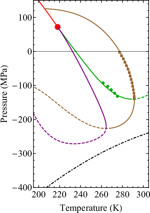
For , Fig. A4 shows a close-up of the lines of anomalies near the spinodal, and Fig. A5 (left) an enlarged view. We see that the model with gives a pattern of lines qualitatively similar to that for a model of real water Caupin and Anisimov 2019 (Fig. A5, right). For , Fig. A6 shows a close-up of the lines of anomalies near the spinodal, with a peculiar feature for : in a narrow pressure range (dashed portion of the green curve), along isobars exhibits successively a maximum, a minimum, and a maximum, as shown in Fig. A7.
References
- Gallo et al. (2016) P. Gallo, K. Amann-Winkel, C. A. Angell, M. A. Anisimov, F. Caupin, C. Chakravarty, E. Lascaris, T. Loerting, A. Z. Panagiotopoulos, J. Russo, J. A. Sellberg, H. E. Stanley, H. Tanaka, C. Vega, L. Xu, and L. G. M. Pettersson, Water: A Tale of Two Liquids, Chem. Rev. 116, 7463 (2016).
- Stanley (2013) H. E. Stanley, Liquid Polymorphism (John Wiley & Sons, 2013).
- Kim et al. (2020) K. H. Kim, K. Amann-Winkel, N. Giovambattista, A. Späh, F. Perakis, H. Pathak, M. L. Parada, C. Yang, D. Mariedahl, T. Eklund, T. J. Lane, S. You, S. Jeong, M. Weston, J. H. Lee, I. Eom, M. Kim, J. Park, S. H. Chun, P. H. Poole, and A. Nilsson, Experimental observation of the liquid-liquid transition in bulk supercooled water under pressure, Science 370, 978 (2020).
- Katayama (2004) Y. Katayama, Macroscopic Separation of Dense Fluid Phase and Liquid Phase of Phosphorus, Science 306, 848 (2004).
- Knudson et al. (2015) M. D. Knudson, M. P. Desjarlais, A. Becker, R. W. Lemke, K. R. Cochrane, M. E. Savage, D. E. Bliss, T. R. Mattsson, and R. Redmer, Direct observation of an abrupt insulator-to-metal transition in dense liquid deuterium, Science 348, 1455 (2015).
- Henry et al. (2020) L. Henry, M. Mezouar, G. Garbarino, D. Sifré, G. Weck, and F. Datchi, Liquid-liquid transition and critical point in sulfur, Nature 584, 382 (2020).
- Xu et al. (2005) L. Xu, P. Kumar, S. V. Buldyrev, S. H. Chen, P. H. Poole, F. Sciortino, and H. E. Stanley, Relation between the Widom line and the dynamic crossover in systems with a liquid–liquid phase transition, Proc. Natl. Acad. Sci. U.S.A. 102, 16558–16562 (2005).
- Vilaseca and Franzese (2011) P. Vilaseca and G. Franzese, Isotropic soft-core potentials with two characteristic length scales and anomalous behaviour, J. Non-Cryst. Solids 357, 419 (2011).
- Pinheiro et al. (2017) L. Pinheiro, A. Furlan, L. Krott, A. Diehl, and M. Barbosa, Critical points, phase transitions and water-like anomalies for an isotropic two length scale potential with increasing attractive well, Physica A 468, 866 (2017).
- Anisimov et al. (2018) M. A. Anisimov, M. Duška, F. Caupin, L. E. Amrhein, A. Rosenbaum, and R. J. Sadus, Thermodynamics of Fluid Polyamorphism, Phys. Rev. X 8, 011004 (2018).
- Tanaka (2000) H. Tanaka, Simple physical model of liquid water, J. Chem. Phys. 112, 799 (2000).
- Holten et al. (2014) V. Holten, J. C. Palmer, P. H. Poole, P. G. Debenedetti, and M. A. Anisimov, Two-state thermodynamics of the ST2 model for supercooled water, J. Chem. Phys. 140, 104502 (2014).
- Singh et al. (2016) R. S. Singh, J. W. Biddle, P. G. Debenedetti, and M. A. Anisimov, Two-state thermodynamics and the possibility of a liquid-liquid phase transition in supercooled TIP4P/2005 water, J. Chem. Phys. 144, 144504 (2016).
- Biddle et al. (2017) J. W. Biddle, R. S. Singh, E. M. Sparano, F. Ricci, M. A. González, C. Valeriani, J. L. F. Abascal, P. G. Debenedetti, M. A. Anisimov, and F. Caupin, Two-structure thermodynamics for the TIP4P/2005 model of water covering supercooled and deeply stretched regions, J. Chem. Phys. 146, 034502 (2017).
- Horstmann and Vogel (2021) R. Horstmann and M. Vogel, Relations between thermodynamics, structures, and dynamics for modified water models in their supercooled regimes, J. Chem. Phys. 154, 054502 (2021).
- Caupin and Anisimov (2019) F. Caupin and M. A. Anisimov, Thermodynamics of supercooled and stretched water: Unifying two-structure description and liquid-vapor spinodal, J. Chem. Phys. 151, 034503 (2019).
- Duška (2020) M. Duška, Water above the spinodal, J. Chem. Phys. 152, 174501 (2020).
- Cheng et al. (2020) B. Cheng, G. Mazzola, C. J. Pickard, and M. Ceriotti, Evidence for supercritical behaviour of high-pressure liquid hydrogen, Nature 585, 217 (2020).
- Holten et al. (2013) V. Holten, D. T. Limmer, V. Molinero, and M. A. Anisimov, Nature of the anomalies in the supercooled liquid state of the mW model of water, J. Chem. Phys. 138, 174501 (2013).
- Sastry et al. (1996) S. Sastry, P. G. Debenedetti, F. Sciortino, and H. E. Stanley, Singularity-free interpretation of the thermodynamics of supercooled water, Phys. Rev. E 53, 6144 (1996).
- Hrubỳ and Holten (2004) J. Hrubỳ and V. Holten, A two-structure model of thermodynamic properties and surface tension of supercooled water, in Proceedings of the 14th International Conference on the Properties of Water and Steam, Kyoto, Japan, Vol. 29 (2004) pp. 241–246.
- Ciach et al. (2008) A. Ciach, W. Góźdź, and A. Perera, Simple three-state lattice model for liquid water, Phys. Rev. E 78, 021203 (2008).
- Stokely et al. (2010) K. Stokely, M. G. Mazza, H. E. Stanley, and G. Franzese, Effect of hydrogen bond cooperativity on the behavior of water, Proc. Natl. Acad. Sci. 107, 1301 (2010).
- Cerdeiriña et al. (2019) C. A. Cerdeiriña, J. Troncoso, D. González-Salgado, P. G. Debenedetti, and H. E. Stanley, Water’s two-critical-point scenario in the Ising paradigm, J. Chem. Phys. 150, 244509 (2019).
- Gibson and Wilding (2006) H. M. Gibson and N. B. Wilding, Metastable liquid-liquid coexistence and density anomalies in a core-softened fluid, Phys. Rev. E 73, 061507 (2006).
- Smallenburg and Sciortino (2015) F. Smallenburg and F. Sciortino, Tuning the Liquid-Liquid Transition by Modulating the Hydrogen-Bond Angular Flexibility in a Model for Water, Phys. Rev. Lett. 115, 015701 (2015).
- Dhabal et al. (2016) D. Dhabal, C. Chakravarty, V. Molinero, and H. K. Kashyap, Comparison of liquid-state anomalies in Stillinger-Weber models of water, silicon, and germanium, J. Chem. Phys. 145, 214502 (2016).
- Russo et al. (2018) J. Russo, K. Akahane, and H. Tanaka, Water-like anomalies as a function of tetrahedrality, PNAS 115, E3333 (2018).
- Trappeniers et al. (1970) N. Trappeniers, J. Schouten, and C. Ten Seldam, Gas-gas equilibrium and the two-component lattice-gas model, Chem. Phys. Lett. 5, 541 (1970).
- Schouten et al. (1974) J. Schouten, C. Ten Seldam, and N. Trappeniers, The two-component lattice-gas model, Physica 73, 556 (1974).
- Furman et al. (1977) D. Furman, S. Dattagupta, and R. B. Griffiths, Global phase diagram for a three-component model, Phys. Rev. B 15, 441 (1977).
- van Konynenburg and Scott (1980) P. H. van Konynenburg and R. L. Scott, Critical lines and phase equilibria in binary van der Waals mixtures, Philos. Trans. R. Soc. A 298, 495 (1980).
- Van Pelt (1992) A. Van Pelt, Critical Phenomena in Binary Fluid Mixtures: Classification of Phase Equilibria with the Simplified-Perturbed-Hard-Chain Theory, Ph.D. thesis, TU Delft, Delft, The Netherlands (1992).
- Tanaka (2020) H. Tanaka, Liquid-liquid transition and polyamorphism, J. Chem. Phys. 153, 130901 (2020).
- Poole et al. (1992) P. H. Poole, F. Sciortino, U. Essmann, and H. E. Stanley, Phase behaviour of metastable water, Nature 360, 324 (1992).
- Poole et al. (1994) P. H. Poole, F. Sciortino, T. Grande, H. E. Stanley, and C. A. Angell, Effect of Hydrogen Bonds on the Thermodynamic Behavior of Liquid Water, Phys. Rev. Lett. 73, 1632 (1994).
- Angell (2008) C. A. Angell, Insights into Phases of Liquid Water from Study of Its Unusual Glass-Forming Properties, Science 319, 582 (2008).
- Chitnelawong et al. (2019) P. Chitnelawong, F. Sciortino, and P. H. Poole, The stability-limit conjecture revisited, J. Chem. Phys. 150, 234502 (2019).
- Debenedetti (2003) P. G. Debenedetti, Supercooled and glassy water, J. Phys. Condens. Matter 15, R1669 (2003).
- Speedy (2004) R. J. Speedy, Comment on “Supercooled and glassy water”, J. Phys. Condens. Matter 16, 6811 (2004).
- Debenedetti (2004) P. G. Debenedetti, Reply to Comment on “Supercooled and glassy water”, J. Phys. Condens. Matter 16, 6815 (2004).
- Holten et al. (2017) V. Holten, C. Qiu, E. Guillerm, M. Wilke, J. Rička, M. Frenz, and F. Caupin, Compressibility Anomalies in Stretched Water and Their Interplay with Density Anomalies, J. Phys. Chem. Lett. 8, 5519 (2017).
- Kim et al. (2017) K. H. Kim, A. Späh, H. Pathak, F. Perakis, D. Mariedahl, K. Amann-Winkel, J. A. Sellberg, J. H. Lee, S. Kim, J. Park, K. H. Nam, T. Katayama, and A. Nilsson, Maxima in the thermodynamic response and correlation functions of deeply supercooled water, Science 358, 1589 (2017).
- Poole et al. (2005) P. H. Poole, I. Saika-Voivod, and F. Sciortino, Density minimum and liquid–liquid phase transition, J. Phys. Condens. Matter 17, L431 (2005).
- Speedy (1982) R. J. Speedy, Stability-limit conjecture. An interpretation of the properties of water, J. Phys. Chem. 86, 982 (1982).
- Franzese et al. (2003) G. Franzese, M. I. Marqués, and H. E. Stanley, Intramolecular coupling as a mechanism for a liquid-liquid phase transition, Phys. Rev. E 67, 011103 (2003).
- Truskett et al. (1999) T. M. Truskett, P. G. Debenedetti, S. Sastry, and S. Torquato, A single-bond approach to orientation-dependent interactions and its implications for liquid water, J. Chem. Phys. 111, 2647 (1999).
- de Oliveira et al. (2009) A. B. de Oliveira, P. A. Netz, and M. C. Barbosa, An ubiquitous mechanism for water-like anomalies, Europhys. Lett. 85, 36001 (2009).
- Urbic (2019) T. Urbic, Modelling water with simple Mercedes-Benz models, Molecular Simulation 45, 279 (2019).
- Bartók et al. (2021) A. P. Bartók, G. Hantal, and L. B. Pártay, Insight into Liquid Polymorphism from the Complex Phase Behavior of a Simple Model, Phys. Rev. Lett. 127, 015701 (2021).
- Clark et al. (2010) G. N. I. Clark, G. L. Hura, J. Teixeira, A. K. Soper, and T. Head-Gordon, Small-angle scattering and the structure of ambient liquid water, Proc. Natl. Acad. Sci. USA 107, 14003 (2010).
- Kiselev and Ely (2002) S. B. Kiselev and J. F. Ely, Parametric crossover model and physical limit of stability in supercooled water, J. Chem. Phys. 116, 5657 (2002).
- Debenedetti et al. (2020) P. G. Debenedetti, F. Sciortino, and G. H. Zerze, Second critical point in two realistic models of water, Science 369, 289 (2020).
- Jedrecy et al. (2021) A. Jedrecy, A. M. Saitta, and F. Pietrucci, Free energy calculations and unbiased dynamics reveal a continuous liquid-liquid transition in water no man’s land, ArXiv210608263 Cond-Mat (2021), arXiv:2106.08263 [cond-mat] .
- Trappeniers and Schouten (1968) N. Trappeniers and J. Schouten, Gas-gas equilibrium in the system neon-krypton, Physics Letters A 27, 340 (1968).
- Rowlinson and Swinton (1982) J. S. Rowlinson and F. L. Swinton, Liquids and Liquid Mixtures (Third Edition), in Liquids and Liquid Mixtures (Third Edition) (Butterworth-Heinemann, 1982).