Destabilization of black holes and stars by generalized Proca fields
Abstract
We demonstrate that black holes and stars in general relativity can be destabilized by perturbations of non-minimally coupled vector fields. Focusing on static and spherically symmetric backgrounds, our analysis shows that black holes with sufficiently small mass and stars with sufficiently high densities are subject to ghost- or gradient-type instabilities. This holds for a large class of Einstein-Proca theories with non-minimal couplings, including generalized Proca models that have sparked attention for their potential role in cosmology and astrophysics. The stability criteria translate into bounds of relevance for low-scale theories of dark energy and for ultra-light dark matter scenarios.
Introduction.—Compact astrophysical objects afford a unique opportunity to probe the existence of new light particles whose couplings to ordinary matter are too weak for direct detection. Observational signatures, including potentially dramatic effects Press 1971; Zel’Dovich 1971; Press and Teukolsky 1972; Damour et al. 1976; Zouros and Eardley 1979; Detweiler 1980; Yoshino and Kodama 2012; Brito et al. 2015, bear the potential to reveal otherwise hidden gravitationally-induced bosonic condensates. Black holes and compact stars thus constitute precious targets for testing particle physics and cosmology via strong-field gravity and multi-messenger astronomy Berti et al. 2015; Cardoso and Pani 2019.
Theory needs to inform experiment by mapping out the “phase diagram” of black holes and compact stars. In a first step, an ambitious research programme drives the development of theoretically consistent bosonic field theories and their interaction with gravity Deffayet and Steer 2013; Langlois 2019; Kobayashi 2019. In a second step, astrophysically relevant solutions are analyzed, asking (i) whether they can account for the observed compact objects and (ii) whether potential instabilities can occur.
Here, we advance the second step and focus on vector bosons Galison and Manohar 1984; Holdom 1986. These are predicted by a number of scenarios beyond the Standard Model Abel et al. 2008; Goodsell et al. 2009 and serve as viable candidates for dark matter Arkani-Hamed and Weiner 2008; Nelson and Scholtz 2011; Arias et al. 2012 and dark energy De Felice et al. 2016a; De Felice et al. 2016b; Beltran Jimenez et al. 2017; de Felice et al. 2017; Heisenberg and Villarrubia-Rojo 2021; Nicosia et al. 2021. If such a light vector particle was to arise from a hidden sector and its dominant interaction with visible matter is mediated by gravity, one is lead to consider Einstein-Proca theory of a massive vector field coupled to gravity. While astrophysical solutions in the minimal version of the theory are constrained by the no-hair theorem Bekenstein 1972a; Bekenstein 1972b, this does not necessarily apply when including non-minimal couplings, i.e., couplings beyond a covariantization of the kinetic term.
The general class of Einstein-Proca theories thus accommodates exotic solutions, including hairy black holes Chagoya et al. 2016; Minamitsuji 2016; Babichev et al. 2017; Heisenberg et al. 2017a; Heisenberg et al. 2017b; Kase et al. 2018a; Kase et al. 2018b, boson stars Minamitsuji 2017 and vectorized stars Nakamura et al. 2017; Kase et al. 2018c; Kase et al. 2020. These may be constrained by current and future observations through the beyond-GR effects of Einstein-Proca theories studied, e.g., in Pani et al. 2012; Witek et al. 2013; Brito et al. 2016; Herdeiro et al. 2016; Sanchis-Gual et al. 2017; Cardoso et al. 2018; Minamitsuji 2018; Sanchis-Gual et al. 2019; Santos et al. 2020; Bustillo et al. 2021; Caputo et al. 2021; Barton et al. 2021.
Nevertheless, all Einstein-Proca theories which admit the same solutions as General Relativity (GR) (supplemented with a vanishing vector-field background) remain unconstrained. In this situation, the crucial phenomenological question thus concerns the stability of GR solutions.
In this letter, we show that Schwarzschild black holes (and stars) destabilize if their mass (inverse density) drops below a threshold value, related to the non-minimal Einstein-Proca couplings. This allows us to either directly constrain the theory or conclude that GR solutions evolve into non-GR solutions with non-vanishing vector field.
Although, in the linearized approximation, it is only the vector field and not the metric which suffers from an instability, the backreaction of the vector beyond linear order is expected to render the whole system unstable. Crucially, the uncovered destabilization differs from what is known as “vectorization” Ramazanoğlu 2017; Ramazanoğlu 2018; Annulli et al. 2019; Minamitsuji 2020a. In analogy to scalarization Damour and Esposito-Farese 1993, vectorization occurs due to tachyonic modes, i.e., wrong-sign mass terms. Here, we find that destabilization is always driven by a ghost or gradient mode, i.e., a wrong-sign kinetic or gradient operator. The latter instability is expected to be far more dramatic than the tachyonic one, with potentially unique astrophysical observables. This calls for numerical-relativity investigations (cf. East and Pretorius 2017; East 2018 for linear Proca fields and Sanchis-Gual et al. 2016; Bosch et al. 2016; Herdeiro et al. 2018; Ripley and Pretorius 2020a; Ripley and Pretorius 2020b; Okounkova 2020; East and Ripley 2021; Silva et al. 2020; Held and Lim 2021 for related numerical studies in other beyond-GR theories), as one may in principle expect a significant signal in gravitational waves sourced by the exponentially growing vector modes beyond linear order.
This novel destabilization channel and the related astrophysical bounds apply to all Einstein-Proca theories with non-minimal couplings that contribute to the linearized dynamics. This includes Generalized Proca (GP) theory Tasinato 2014; Heisenberg 2014; Hull et al. 2016 which has received much attention recently in studies of dark matter and dark energy, as well as on the potential role of new light particles in astrophysical phenomena. We find that destabilization of stellar-mass Schwarzschild black holes constrains cosmological models in which the associated non-minimal coupling is set by the energy scale , where is the Planck scale and is the Hubble constant. Moreover, if stellar mass black holes acquire transient charges Wald 1974; Levin et al. 2018, destabilization could also constrain fuzzy dark-matter models Hu et al. 2000.
General quadratic Lagrangian.—We consider a metric tensor and vector field with an action
| (1) |
Here and are the two constant parameters that define the model, is the Planck mass and is the mass of the vector field (we assume ). For instance, Eq. (Destabilization of black holes and stars by generalized Proca fields) follows from expanding the complete GP theory to quadratic order in the vector field about on an arbitrary curved background (see Supplemental Material A).
GP is the complete generalization of the standard Proca theory, i.e., its interactions preserve the existence of a (local) frame in which the component is non-dynamical. Although sufficient, this is not necessary for consistency with respect to the number of degrees of freedom Errasti Díez et al. 2020a; Errasti Díez et al. 2020b, see Heisenberg et al. 2016; Kimura et al. 2017; de Rham and Pozsgay 2020 for alternative extensions. Nevertheless, eq. (Destabilization of black holes and stars by generalized Proca fields) is the most general vector-tensor model that is (i) quadratic in the vector field, (ii) a function of the vector field and its first derivative only, (iii) at most linear in the undifferentiated curvature.
Condition (i) follows because we are investigating the linear stability of GR solutions without vector condensate. Condition (ii) is a sufficient condition to avoid extra degrees of freedom as in GP theory. Condition (iii) is motivated by our focus on astrophysical GR backgrounds with subleading higher-derivative terms.
Stability and quasi-normal modes of a minimally-coupled Proca field on black-hole spacetimes are studied in Konoplya 2006; Rosa and Dolan 2012; Baumann et al. 2019; Percival and Dolan 2020. The coupling proportional to the Einstein tensor was considered previously e.g. in Chagoya et al. 2016; Minamitsuji 2016; Babichev et al. 2017, although restricted to unperturbed backgrounds. The interaction terms involving the field strength, which are reminiscent of the Drummond-Hathrell effective action Drummond and Hathrell 1980, were studied in Beltran Jimenez et al. 2013. We confirm their results on the stability of GR black holes as a special case of our more general setup.
Stability conditions.—We focus on static and spherically symmetric backgrounds, for which the metric can be chosen as
| (2) |
Perturbations of the metric about GR backgrounds with vanishing vector field decouple and can be ignored. The vector field can be decomposed in vector spherical harmonics (see e.g. Nollert 1999),
| (3) |
Explicit expressions for are given in Supplemental Material B. The mode functions with correspond to perturbations with polar parity while corresponds to an axial-parity mode. Parity is a “good quantum number”. Hence, polar and axial perturbations decouple at linear order.
The stability of localized perturbations—with physical size much smaller than all the length scales of the background—is dictated by the structure of the causal cones (see de Rham and Melville 2017; Babichev et al. 2018; de Rham and Zhang 2019; de Rham et al. 2020 for related discussions). In other words, to address the question of local stability one may neglect background variations and evaluate all metric functions at fixed radius . The propagator matrix for the mode functions is defined in Fourier space. Gradient and tachyonic instabilities can be determined by the dispersion relations, defined by the poles of the inverse propagator matrix. The presence of ghosts follows from the matrix of residues. See Supplemental Material C for details. Henceforth, we drop the subscript on the fixed radius .
The axial sector has a single degree of freedom. Its dispersion relation follows from the decomposed action,
| (4) |
where and are the comoving (as opposed to proper) frequency and radial wave number, and
| (5) | ||||
Here, a prime denotes differentiation with respect to . The curvature terms and are known in terms of and .
For , only two combinations of the three polar mode functions are dynamical. Integrating out the non-dynamical mode, see Supplemental Material B, we can infer the 2-by-2 (inverse) propagator matrix . Its components read
| (6) | ||||
Here , and
| (7) | ||||
The dispersion relations are defined by the roots of the equation .
Monopole perturbations with are special in that only is present in the polar sector. Its dispersion relation reads
| (8) |
Notice that the dispersion relations of the polar and axial sector involve the same functions , and . A priori these functions need not be in any way related—in fact they are not for the monopole modes. This coincidence has important consequences for the stability conditions.
The stability of axial perturbations under ghosts and radial gradients dictates that and for all physical radii. Stability of these modes under angular gradients, which means that must be positive in the limit , requires . Similarly, stability of the polar monopole mode implies that and . Given these conditions, it then follows that all polar modes with are stable under ghosts and radial gradients, see Supplemental Material C. Further, the stability of these modes under angular gradients gives independent constraints, namely and . In turn, these last two conditions imply the absence of tachyonic instabilities for all the perturbations.
An important outcome is that tachyon-like instabilities are absent—for if such modes are excited, they are necessarily accompanied by ghosts and/or gradient-unstable modes with a much faster growth rate. Hence, vector condensates cannot form as a result of a standard vectorization mechanism—which by definition follows from a tachyon- or Jeans-type destabilization—starting from any static spherically symmetric GR state and for any Einstein-Proca theory that reduces to eq. (Destabilization of black holes and stars by generalized Proca fields) at linear order.
Black holes.—For the Schwarzschild black hole (BH) of mass , i.e., for with , the stability conditions simplify. Whenever holds, and and the propagator matrix in eq. (6) is diagonal. Moreover, for vacuum GR solutions, the dependence on drops out; cf. eq. (Destabilization of black holes and stars by generalized Proca fields). For the Schwarzschild spacetime, one finds that are automatically positive, while and . Positivity of these functions for all requires
| (9) |
in order for Schwarzschild BHs to be stable. This bound is in agreement with the results of Beltran Jimenez et al. 2013. It implies that small enough BHs are always unstable whenever is non-zero.
Order-of-magnitude estimates (assuming validity of the vector theory on all involved scales) reveal that the stability bound in eq. (9) could be of relevance both in late-time cosmology as well as for primordial BHs. In the cosmological setting, non-linear operators are typically controlled by an energy scale , where is the Hubble constant Nicolis and Rattazzi 2004; Nicolis et al. 2009.11 1 This estimate is based on scalar-tensor theories and implicitly assumes the existence of a decoupling limit in which the vector-tensor models we consider can be approximated by scalar-tensor interactions. Taking, for example, , this yields , implying the destabilization of stellar-mass BHs while supermassive BHs remain stable. For smaller values of , stellar-mass BHs remain stable while primordial BHs in the experimentally preferred range Carr et al. 2020 would still be subject to the instability.
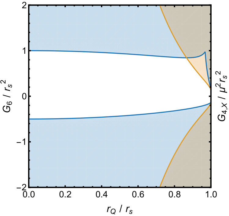
Constraining the parameter requires to look at non-Ricci-flat GR solutions. We consider the Reissner-Nordström (RN) metric as a first example. Although astrophysical BHs are unlikely to exhibit significant electric (or magnetic) charge, small and transient charges remain viable. For instance, stellar-mass BHs could accrete charges up to of order , in units of the BH mass Levin et al. 2018, through the Wald mechanism Wald 1974 in a merger with a strongly magnetized neutron star.22 2 In Wald 1974; Levin et al. 2018, the charging effect requires a spinning BH, however, a more recent study Chen and Dai 2021 has shown that rotation is not needed and that the relative motion between the coalescing BH and neutron star can generate charges of comparable magnitude.
The RN metric is defined by . Here, in terms of the hole’s electric charge and we recall the extremality bound . The stability conditions now depend on the scale , cf. fig. 1, and Supplemental Material D for the analytic expressions. For , we observe a non-trivial dependence of the stability bounds on the charge, cf. Beltran Jimenez et al. 2013; in particular, they are most restrictive for an extremal BH, for which .
More interestingly, we find a novel bound on ,
| (10) |
Remarkably, for any fixed , , and , this bound implies a lower limit on the vector-boson mass . As a concrete example, for , as typically considered in the literature, stability of a stellar-mass BH with that acquires the aforementioned estimate implies as the critical vector-boson mass. Comparison with the typical mass range for fuzzy dark matter Hu et al. 2000 exemplifies the significance of eq. (10) for the study of ultra-light particles. We note that may not be independent of : if the operators that break gauge invariance were to arise from a Higgs-type mechanism, we would expect de Rham et al. 2019 and our stability criteria would not directly constrain the mass but rather the scale of symmetry breaking.
Stars.—We have analyzed the stability conditions for static perfect fluid stars governed by the TOV equations. Although for generic equations of state (EoS)—relating the pressure to the density —the metric cannot be determined in analytic form, critical values for the parameters and can still be obtained if one assumes that the functions that determine the stability are minimized at the center of the star. We have checked analytically that this assumption is correct for a uniform-density star, and also numerically for a polytropic star with EoS , see Supplemental Material D. It is plausible that the assumption is true for all realistic EoS, including ones for imperfect fluids, and we plan to come back to this question in a dedicated work.
Under this premise, we can infer the following bounds on the GP coupling constants:
| (11) |
where and are the pressure and density at the center. Fig. 2 shows the critical values of and for stellar models with uniform-density and polytropic EoS, plotted as functions of the normalized star’s radius. We observe an interesting dependence on the EoS, with the bounds for a polytrope being up to three orders of magnitude stronger than for a uniform-density star with the same central pressure and density.
The stability window for both coupling parameters shrinks to zero as the star’s central pressure and density increase. For a neutron star with one has if we take . This bound on may seem mild but again could be violated in very low-scale models like the ones envisioned in cosmology and in the context of ultra-light dark matter.
Discussion.—We identify a novel destabilization channel for static and spherically-symmetric GR backgrounds triggered by non-minimally coupled vector perturbations. Any non-vanishing non-minimal coupling destabilizes small enough BHs and dense enough stars. The implied astrophysical constraints ultimately depend on the scales at hand. We find relevant constraints for theories of dark energy and ultra-light dark matter. The non-minimal couplings that source destabilization, cf. eq. (Destabilization of black holes and stars by generalized Proca fields), naturally appear in all of these scenarios, unless the model is fine-tuned to avoid them.
More specifically, avoiding instabilities of stellar-mass BHs and/or neutron stars constrains the respective non-minimal coupling at cosmologically relevant scales set by , with the Planck scale and the Hubble constant. In turn, transient charges, potentially induced by nearby strongly magnetized neutron stars, imply further destabilization constraints involving the Proca mass and are of relevance for ultra-light vector dark-matter models.
Notably, destabilization differs from vectorization. The latter describes a transition between GR and non-GR solutions via a tachyonic growth mode. Here, we find that a potential tachyonic instability is always accompanied by a dominant ghost or gradient instability. Hence, destabilization is controlled by the highest growth rates in the problem. The timescale and fate of the instability thus remain uncertain.
We emphasize that the destabilization channel concerns only GR solutions and does not constrain solutions with non-trivial vector hair. Formally, we have only shown a linear instability in the vector field, and not in the metric. However, as one may expect for ghost/gradient modes, interactions beyond linear order will generically destabilize the full system. Future non-linear studies are necessary to strictly discard the possibility that the vector field may settle into a condensed state with the GR metric being kept intact, as it occurs with so-called “stealth” solutions Babichev and Charmousis 2014; Chagoya and Tasinato 2018; Minamitsuji and Motohashi 2018; Minamitsuji 2020b.
From the perspective of radiative corrections, the inclusion of higher-derivative operators may quench the instability, similarly to the phenomenon of ghost condensation Arkani-Hamed et al. 2004. This possibility calls for a detailed study to determine the role of higher-order operators. Assuming the transition can be made sense of in a controlled theoretical framework, our analysis makes a strong case for simulating Einstein-Proca theories in numerical relativity.
There are also several avenues for future work within the present set-up of linear perturbations about GR backgrounds. This includes (i) studying a broader set of stellar models in order to verify the robustness of our bounds in eq. (11); (ii) effects of a cosmological constant, potentially related to extended vector fields in holographic models (see e.g. Jing and Chen 2010; Jing et al. 2011; Zhao et al. 2013); and, of course, (iii) an extension to non-static systems, in particular rotating BHs and stars.
Acknowledgments.—We would like to thank Claudia de Rham, Lavinia Heisenberg, Shinji Mukohyama and an anonymous referee for useful comments. SGS and JZ are supported by the European Union’s Horizon 2020 Research Council grant 724659 MassiveCosmo ERC-2016-COG. AH is supported by a Royal Society Newton International fellowship [NIF\R1\191008].
Appendix A Generalized Proca Lagrangian
The Lagrangian of Generalized Proca (GP) theory in four dimensions is defined as Tasinato 2014; Heisenberg 2014
| (12) | ||||
where
| (13) | ||||
with the definitions
| (14) |
The expression means the derivative of the function with respect to its argument, and similarly for and . Note that in (12) we have written explicitly the Einstein-Hilbert and Proca Lagrangians so that we may take . Observe also that and multiply total derivatives and may be ignored in a perturbative expansion in powers of the vector field.
Expanding the full action to quadratic order in and its derivative gives eq. (Destabilization of black holes and stars by generalized Proca fields) in the main text after one notices that
| (15) |
(“t.d.” means total derivative) and
| (16) | ||||
The conclusion is that the GP Lagrangian reduces, when truncated to quadratic order in the vector field, to the standard Proca theory plus a sum of non-minimal couplings involving , and the curvature tensor. These non-minimal coupling terms must appear in specific combinations—proportional to the Einstein tensor and the dual Riemann tensor—in order to avoid additional degrees of freedom.
We mentioned in the main text that other extensions of the linear Proca theory will not give additional operators within the framework specified by our assumptions. This is clear for the models proposed in Heisenberg et al. 2016; Kimura et al. 2017 which modify GP theory with terms that do not contribute at quadratic order. On the other hand, the model of de Rham and Pozsgay 2020 is genuinely independent from GP (in the sense that the Lagrangians cannot be matched by any choice of parameters); nevertheless, when expanded to quadratic order the two models are not inequivalent and hence the proposal of de Rham and Pozsgay 2020 does fall within our class once complemented with appropriate non-minimal curvature couplings.
Appendix B Expansion of the action in spherical harmonics
B.1 Vector spherical harmonics
The decomposition of the Proca field in vector spherical harmonics is given in eq. (3) in the main text. In our conventions the vector harmonic functions are given by
| (17) | ||||
with denoting the standard spherical harmonic functions which solve the Laplace equation on the sphere,
| (18) |
The three functions have polar or even parity, i.e. they acquire a factor under space inversions , while has axial or odd parity, acquiring a factor under inversions.
We recall the basic orthogonality property of the spherical harmonics,
| (19) |
and also that . It then follows that the 4-vector spherical harmonics, with the normalization given above, satisfy
| (20) |
the inner product being defined by the matrix . The vector spherical harmonics also inherit the conjugation property,
| (21) |
The reality of the field then implies that .
B.2 Axial perturbations
Expanding the complete Lagrangian in terms of the mode functions we obtain the following result for the axial sector:
| (22) | ||||
with the functions , , and as defined in the main text.
B.3 Polar perturbations
The Lagrangian for the polar perturbations , and is given by
| (23) | ||||
and the functions , and can be found in the Letter.
This Lagrangian is degenerate in the sense that not all among the three mode functions are dynamical and, as explained in the text, it is useful to integrate out the non-dynamical mode. The monopole sector with is preculiar because , so we start by treating this case separately. The trick is to introduce the auxiliary field
| (24) |
with . This can then be incorporated in the Lagrangian as
| (25) | ||||
with . Variation with respect to gives (24), which may be substituted back to recover the original action, proving that the two are indeed equivalent. Alternatively, from the latter form of the action we can integrate out and since now their eqs. of motion are algebraic:
| (26) | ||||
and we obtain
| (27) | ||||
for the Lagrangian describing the dynamics of the monopole polar mode.
For generic higher multipoles we can carry out the same procedure in order to remove the non-dynamical mode. We define
| (28) |
and solving for and from their eqs. of motion now yields
| (29) | ||||
Substituting back in the action we eventually find
| (30) | ||||
which as claimed contains two dynamical modes for each .
Appendix C Stability conditions and matrix of propagators
Consider a fully generic two-derivative quadratic Lagrangian,
| (31) |
The fields are not necessarily scalars, i.e. they may be components of a set of tensor fields. The coordinates are not necessarily Cartesian, although we are primarily interested in the situation where is timelike and is spacelike. In principle the tensor may be a function of the coordinates, but for the purpose of determining the presence of ghost and gradient-type instabilities it suffices to assume it is a constant as we explained in the main text.
The inverse Fourier-space propagator is
| (32) |
Inverting gives the propagator , more precisely the matrix of propagators. The poles of correspond to the physical particles. By “poles” of a matrix we mean the values of for which the inverse determinant vanishes. Thus the dispersion relations, which determine the particle spectrum and the causal cone structure, are given by the solutions of
| (33) |
Gradient instabilities can be determined unambiguously from the dispersion relations. Ghost instabilities, on the other hand, are ambiguous in that they make reference to the orientation of the causal cones relative to another reference particle sector, which is by assumption “healthy”. If we take this reference sector to be an ordinary scalar field (but any garden-variety field would do),
| (34) |
its propagator, as defined above, is obviously . The dispersion relation is given by the pole, , and there is of course no gradient instability.
Upon quantization, the norms of the physical modes are inferred from the residues of the propagator at the particles’ poles. The signs of the norms are conventional—only the relative signs are important. We choose to define our reference field to have unit norm, and therefore the residue matrix from which the norms are inferred must be given by
| (35) |
where is the -th pole of the propagator.
For our reference field we then clearly have , as desired. Because this field is by definition “healthy”, any other dynamical mode having a negative residue (more precisely, a residue matrix with one or more negative eigenvalues) is by definition a ghost.
Let us apply this to the following 2D toy model:
| (36) |
For generic parameters, this Lagrangian cannot be diagonalized via a local field redefinition (in particular, such a redefinition does not exist whenever ). But as we have explained, the particle spectrum and its stability can be determined from the propagator alone. Comparing (36) and (30) we see that this actually serves as a proxy model for the polar Lagrangian that we sought to analyze.
In the field basis we have
| (37) |
so that
| (38) |
with determinant
| (39) | ||||
and for the roots we find
| (40) |
Absence of gradient-unstable modes means that these solutions must be positive (a solution with would signal a degeneracy; we ignore this possibility as it would require a separate analysis). This restricts the parameters by the inequalities
| (41) |
Next we define the residue matrices,
| (42) | ||||
By construction these matrices have zero determinant, meaning that each has a single non-zero eigenvalue and so there are two non-zero norms, as expected. We find these to be
| (43) |
Clearly the stable-gradients condition ensures that , but the condition gives an independent constraint,
| (44) | ||||
This is automatically satisfied if , but is otherwise non-trivial. Note also that this inequality implies the second one in (41) but is more restrictive than it.
Appendix D Analysis of stability conditions
As explained in the Letter, the stability of the system under consideration hinges on the signs of the functions , , , , , and defined in eqs. (5) and (7). According to our stability criteria, these functions must all be positive definite in the domain of interest, translating into bounds on and . We next provide these bounds for the RN and TOV metrics that we focused on in the Letter.
D.1 Reissner-Nordström metric
For the RN spacetime the domain of interest is , with the location of the event horizon being given by . Table 1 displays the conditions for the functions determining the stability criteria to be positive definite (recall that and for the RN metric).
| Function | Condition for positive definiteness |
|---|---|
D.2 TOV metric
The TOV metric components are given by
| (45) |
where here and below all tilde variables correspond to quantities normalized by an arbitrary mass scale and associated distance scale ; this is of course not necessary but is convenient in order to only deal with dimensionless variables in numerical computations.
The functions and , along with the pressure , are determined by the TOV equations
| (46) | ||||
Assuming regularity at the star’s center, , one can solve these equations in power series to find
| (47) | ||||
where and are to be obtained from the equation of state . It is then straightforward to evaluate the stability criteria at in order to derive the bounds quoted in the main text.
References
- Press (1971) W. H. Press, Astrophys. J. Lett. 170, L105 (1971).
- Zel’Dovich (1971) Y. B. Zel’Dovich, Soviet Journal of Experimental and Theoretical Physics Letters 14, 180 (1971).
- Press and Teukolsky (1972) W. H. Press and S. A. Teukolsky, Nature 238, 211 (1972).
- Damour et al. (1976) T. Damour, N. Deruelle, and R. Ruffini, Lett. Nuovo Cim. 15, 257 (1976).
- Zouros and Eardley (1979) T. J. M. Zouros and D. M. Eardley, Annals Phys. 118, 139 (1979).
- Detweiler (1980) S. L. Detweiler, Phys. Rev. D 22, 2323 (1980).
- Yoshino and Kodama (2012) H. Yoshino and H. Kodama, Prog. Theor. Phys. 128, 153 (2012), arXiv:1203.5070 [gr-qc] .
- Brito et al. (2015) R. Brito, V. Cardoso, and P. Pani, Lect. Notes Phys. 906, pp.1 (2015), arXiv:1501.06570 [gr-qc] .
- Berti et al. (2015) E. Berti et al., Class. Quant. Grav. 32, 243001 (2015), arXiv:1501.07274 [gr-qc] .
- Cardoso and Pani (2019) V. Cardoso and P. Pani, Living Rev. Rel. 22, 4 (2019), arXiv:1904.05363 [gr-qc] .
- Deffayet and Steer (2013) C. Deffayet and D. A. Steer, Class. Quant. Grav. 30, 214006 (2013), arXiv:1307.2450 [hep-th] .
- Langlois (2019) D. Langlois, Int. J. Mod. Phys. D 28, 1942006 (2019), arXiv:1811.06271 [gr-qc] .
- Kobayashi (2019) T. Kobayashi, Rept. Prog. Phys. 82, 086901 (2019), arXiv:1901.07183 [gr-qc] .
- Galison and Manohar (1984) P. Galison and A. Manohar, Phys. Lett. B 136, 279 (1984).
- Holdom (1986) B. Holdom, Phys. Lett. B 166, 196 (1986).
- Abel et al. (2008) S. A. Abel, M. D. Goodsell, J. Jaeckel, V. V. Khoze, and A. Ringwald, JHEP 07, 124 (2008), arXiv:0803.1449 [hep-ph] .
- Goodsell et al. (2009) M. Goodsell, J. Jaeckel, J. Redondo, and A. Ringwald, JHEP 11, 027 (2009), arXiv:0909.0515 [hep-ph] .
- Arkani-Hamed and Weiner (2008) N. Arkani-Hamed and N. Weiner, JHEP 12, 104 (2008), arXiv:0810.0714 [hep-ph] .
- Nelson and Scholtz (2011) A. E. Nelson and J. Scholtz, Phys. Rev. D 84, 103501 (2011), arXiv:1105.2812 [hep-ph] .
- Arias et al. (2012) P. Arias, D. Cadamuro, M. Goodsell, J. Jaeckel, J. Redondo, and A. Ringwald, JCAP 06, 013 (2012), arXiv:1201.5902 [hep-ph] .
- De Felice et al. (2016a) A. De Felice, L. Heisenberg, R. Kase, S. Mukohyama, S. Tsujikawa, and Y.-l. Zhang, JCAP 06, 048 (2016a), arXiv:1603.05806 [gr-qc] .
- De Felice et al. (2016b) A. De Felice, L. Heisenberg, R. Kase, S. Mukohyama, S. Tsujikawa, and Y.-l. Zhang, Phys. Rev. D 94, 044024 (2016b), arXiv:1605.05066 [gr-qc] .
- Beltran Jimenez et al. (2017) J. Beltran Jimenez, L. Heisenberg, R. Kase, R. Namba, and S. Tsujikawa, Phys. Rev. D 95, 063533 (2017), arXiv:1702.01193 [hep-th] .
- de Felice et al. (2017) A. de Felice, L. Heisenberg, and S. Tsujikawa, Phys. Rev. D 95, 123540 (2017), arXiv:1703.09573 [astro-ph.CO] .
- Heisenberg and Villarrubia-Rojo (2021) L. Heisenberg and H. Villarrubia-Rojo, JCAP 03, 032 (2021), arXiv:2010.00513 [astro-ph.CO] .
- Nicosia et al. (2021) G.-P. Nicosia, J. Levi Said, and V. Gakis, Eur. Phys. J. Plus 136, 191 (2021), arXiv:2012.11959 [gr-qc] .
- Bekenstein (1972a) J. D. Bekenstein, Phys. Rev. D 5, 1239 (1972a).
- Bekenstein (1972b) J. D. Bekenstein, Phys. Rev. Lett. 28, 452 (1972b).
- Chagoya et al. (2016) J. Chagoya, G. Niz, and G. Tasinato, Class. Quant. Grav. 33, 175007 (2016), arXiv:1602.08697 [hep-th] .
- Minamitsuji (2016) M. Minamitsuji, Phys. Rev. D 94, 084039 (2016), arXiv:1607.06278 [gr-qc] .
- Babichev et al. (2017) E. Babichev, C. Charmousis, and M. Hassaine, JHEP 05, 114 (2017), arXiv:1703.07676 [gr-qc] .
- Heisenberg et al. (2017a) L. Heisenberg, R. Kase, M. Minamitsuji, and S. Tsujikawa, Phys. Rev. D 96, 084049 (2017a), arXiv:1705.09662 [gr-qc] .
- Heisenberg et al. (2017b) L. Heisenberg, R. Kase, M. Minamitsuji, and S. Tsujikawa, JCAP 08, 024 (2017b), arXiv:1706.05115 [gr-qc] .
- Kase et al. (2018a) R. Kase, M. Minamitsuji, S. Tsujikawa, and Y.-L. Zhang, JCAP 02, 048 (2018a), arXiv:1801.01787 [gr-qc] .
- Kase et al. (2018b) R. Kase, M. Minamitsuji, and S. Tsujikawa, Phys. Lett. B 782, 541 (2018b), arXiv:1803.06335 [gr-qc] .
- Minamitsuji (2017) M. Minamitsuji, Phys. Rev. D 96, 044017 (2017), arXiv:1708.05358 [gr-qc] .
- Nakamura et al. (2017) S. Nakamura, R. Kase, and S. Tsujikawa, Phys. Rev. D 96, 084005 (2017), arXiv:1707.09194 [gr-qc] .
- Kase et al. (2018c) R. Kase, M. Minamitsuji, and S. Tsujikawa, Phys. Rev. D 97, 084009 (2018c), arXiv:1711.08713 [gr-qc] .
- Kase et al. (2020) R. Kase, M. Minamitsuji, and S. Tsujikawa, Phys. Rev. D 102, 024067 (2020), arXiv:2001.10701 [gr-qc] .
- Pani et al. (2012) P. Pani, V. Cardoso, L. Gualtieri, E. Berti, and A. Ishibashi, Phys. Rev. Lett. 109, 131102 (2012), arXiv:1209.0465 [gr-qc] .
- Witek et al. (2013) H. Witek, V. Cardoso, A. Ishibashi, and U. Sperhake, Phys. Rev. D 87, 043513 (2013), arXiv:1212.0551 [gr-qc] .
- Brito et al. (2016) R. Brito, V. Cardoso, C. A. R. Herdeiro, and E. Radu, Phys. Lett. B 752, 291 (2016), arXiv:1508.05395 [gr-qc] .
- Herdeiro et al. (2016) C. Herdeiro, E. Radu, and H. Rúnarsson, Class. Quant. Grav. 33, 154001 (2016), arXiv:1603.02687 [gr-qc] .
- Sanchis-Gual et al. (2017) N. Sanchis-Gual, C. Herdeiro, E. Radu, J. C. Degollado, and J. A. Font, Phys. Rev. D 95, 104028 (2017), arXiv:1702.04532 [gr-qc] .
- Cardoso et al. (2018) V. Cardoso, O. J. C. Dias, G. S. Hartnett, M. Middleton, P. Pani, and J. E. Santos, JCAP 03, 043 (2018), arXiv:1801.01420 [gr-qc] .
- Minamitsuji (2018) M. Minamitsuji, Phys. Rev. D 97, 104023 (2018), arXiv:1805.09867 [gr-qc] .
- Sanchis-Gual et al. (2019) N. Sanchis-Gual, C. Herdeiro, J. A. Font, E. Radu, and F. Di Giovanni, Phys. Rev. D 99, 024017 (2019), arXiv:1806.07779 [gr-qc] .
- Santos et al. (2020) N. M. Santos, C. L. Benone, L. C. B. Crispino, C. A. R. Herdeiro, and E. Radu, JHEP 07, 010 (2020), arXiv:2004.09536 [gr-qc] .
- Bustillo et al. (2021) J. C. Bustillo, N. Sanchis-Gual, A. Torres-Forné, J. A. Font, A. Vajpeyi, R. Smith, C. Herdeiro, E. Radu, and S. H. W. Leong, Phys. Rev. Lett. 126, 081101 (2021), arXiv:2009.05376 [gr-qc] .
- Caputo et al. (2021) A. Caputo, S. J. Witte, D. Blas, and P. Pani, (2021), arXiv:2102.11280 [hep-ph] .
- Barton et al. (2021) S. Barton, B. Hartmann, B. Kleinhaus, and J. Kunz, (2021), arXiv:2103.01651 [gr-qc] .
- Ramazanoğlu (2017) F. M. Ramazanoğlu, Phys. Rev. D 96, 064009 (2017), arXiv:1706.01056 [gr-qc] .
- Ramazanoğlu (2018) F. M. Ramazanoğlu, Phys. Rev. D 98, 044013 (2018), arXiv:1804.03158 [gr-qc] .
- Annulli et al. (2019) L. Annulli, V. Cardoso, and L. Gualtieri, Phys. Rev. D 99, 044038 (2019), arXiv:1901.02461 [gr-qc] .
- Minamitsuji (2020a) M. Minamitsuji, Phys. Rev. D 101, 104044 (2020a), arXiv:2003.11885 [gr-qc] .
- Damour and Esposito-Farese (1993) T. Damour and G. Esposito-Farese, Phys. Rev. Lett. 70, 2220 (1993).
- East and Pretorius (2017) W. E. East and F. Pretorius, Phys. Rev. Lett. 119, 041101 (2017), arXiv:1704.04791 [gr-qc] .
- East (2018) W. E. East, Phys. Rev. Lett. 121, 131104 (2018), arXiv:1807.00043 [gr-qc] .
- Sanchis-Gual et al. (2016) N. Sanchis-Gual, J. C. Degollado, P. J. Montero, J. A. Font, and C. Herdeiro, Phys. Rev. Lett. 116, 141101 (2016), arXiv:1512.05358 [gr-qc] .
- Bosch et al. (2016) P. Bosch, S. R. Green, and L. Lehner, Phys. Rev. Lett. 116, 141102 (2016), arXiv:1601.01384 [gr-qc] .
- Herdeiro et al. (2018) C. A. R. Herdeiro, E. Radu, N. Sanchis-Gual, and J. A. Font, Phys. Rev. Lett. 121, 101102 (2018), arXiv:1806.05190 [gr-qc] .
- Ripley and Pretorius (2020a) J. L. Ripley and F. Pretorius, Phys. Rev. D101, 044015 (2020a), arXiv:1911.11027 [gr-qc] .
- Ripley and Pretorius (2020b) J. L. Ripley and F. Pretorius, Class. Quant. Grav. 37, 155003 (2020b), arXiv:2005.05417 [gr-qc] .
- Okounkova (2020) M. Okounkova, Phys. Rev. D102, 084046 (2020), arXiv:2001.03571 [gr-qc] .
- East and Ripley (2021) W. E. East and J. L. Ripley, Phys. Rev. D103, 044040 (2021), arXiv:2011.03547 [gr-qc] .
- Silva et al. (2020) H. O. Silva, H. Witek, M. Elley, and N. Yunes, (2020), arXiv:2012.10436 [gr-qc] .
- Held and Lim (2021) A. Held and H. Lim, (2021), arXiv:2104.04010 [gr-qc] .
- Tasinato (2014) G. Tasinato, JHEP 04, 067 (2014), arXiv:1402.6450 [hep-th] .
- Heisenberg (2014) L. Heisenberg, JCAP 05, 015 (2014), arXiv:1402.7026 [hep-th] .
- Hull et al. (2016) M. Hull, K. Koyama, and G. Tasinato, Phys. Rev. D 93, 064012 (2016), arXiv:1510.07029 [hep-th] .
- Wald (1974) R. M. Wald, Phys. Rev. D 10, 1680 (1974).
- Levin et al. (2018) J. Levin, D. J. D’Orazio, and S. Garcia-Saenz, Phys. Rev. D 98, 123002 (2018), arXiv:1808.07887 [astro-ph.HE] .
- Hu et al. (2000) W. Hu, R. Barkana, and A. Gruzinov, Phys. Rev. Lett. 85, 1158 (2000), arXiv:astro-ph/0003365 .
- Errasti Díez et al. (2020a) V. Errasti Díez, B. Gording, J. A. Méndez-Zavaleta, and A. Schmidt-May, Phys. Rev. D 101, 045009 (2020a), arXiv:1905.06968 [hep-th] .
- Errasti Díez et al. (2020b) V. Errasti Díez, B. Gording, J. A. Méndez-Zavaleta, and A. Schmidt-May, Phys. Rev. D 101, 045008 (2020b), arXiv:1905.06967 [hep-th] .
- Heisenberg et al. (2016) L. Heisenberg, R. Kase, and S. Tsujikawa, Phys. Lett. B 760, 617 (2016), arXiv:1605.05565 [hep-th] .
- Kimura et al. (2017) R. Kimura, A. Naruko, and D. Yoshida, JCAP 01, 002 (2017), arXiv:1608.07066 [gr-qc] .
- de Rham and Pozsgay (2020) C. de Rham and V. Pozsgay, Phys. Rev. D 102, 083508 (2020), arXiv:2003.13773 [hep-th] .
- Konoplya (2006) R. A. Konoplya, Phys. Rev. D 73, 024009 (2006), arXiv:gr-qc/0509026 .
- Rosa and Dolan (2012) J. G. Rosa and S. R. Dolan, Phys. Rev. D 85, 044043 (2012), arXiv:1110.4494 [hep-th] .
- Baumann et al. (2019) D. Baumann, H. S. Chia, J. Stout, and L. ter Haar, JCAP 12, 006 (2019), arXiv:1908.10370 [gr-qc] .
- Percival and Dolan (2020) J. Percival and S. R. Dolan, Phys. Rev. D 102, 104055 (2020), arXiv:2008.10621 [gr-qc] .
- Drummond and Hathrell (1980) I. T. Drummond and S. J. Hathrell, Phys. Rev. D 22, 343 (1980).
- Beltran Jimenez et al. (2013) J. Beltran Jimenez, R. Durrer, L. Heisenberg, and M. Thorsrud, JCAP 10, 064 (2013), arXiv:1308.1867 [hep-th] .
- Nollert (1999) H.-P. Nollert, Class. Quant. Grav. 16, R159 (1999).
- de Rham and Melville (2017) C. de Rham and S. Melville, Phys. Rev. D 95, 123523 (2017), arXiv:1703.00025 [hep-th] .
- Babichev et al. (2018) E. Babichev, C. Charmousis, G. Esposito-Farèse, and A. Lehébel, Phys. Rev. D 98, 104050 (2018), arXiv:1803.11444 [gr-qc] .
- de Rham and Zhang (2019) C. de Rham and J. Zhang, Phys. Rev. D 100, 124023 (2019), arXiv:1907.00699 [hep-th] .
- de Rham et al. (2020) C. de Rham, J. Francfort, and J. Zhang, Phys. Rev. D 102, 024079 (2020), arXiv:2005.13923 [hep-th] .
- Nicolis and Rattazzi (2004) A. Nicolis and R. Rattazzi, JHEP 06, 059 (2004), arXiv:hep-th/0404159 .
- Nicolis et al. (2009) A. Nicolis, R. Rattazzi, and E. Trincherini, Phys. Rev. D 79, 064036 (2009), arXiv:0811.2197 [hep-th] .
- Carr et al. (2020) B. Carr, K. Kohri, Y. Sendouda, and J. Yokoyama, (2020), arXiv:2002.12778 [astro-ph.CO] .
- Chen and Dai (2021) K. Chen and Z. G. Dai, Astrophys. J. 909, 4 (2021).
- de Rham et al. (2019) C. de Rham, S. Melville, A. J. Tolley, and S.-Y. Zhou, JHEP 03, 182 (2019), arXiv:1804.10624 [hep-th] .
- Babichev and Charmousis (2014) E. Babichev and C. Charmousis, JHEP 08, 106 (2014), arXiv:1312.3204 [gr-qc] .
- Chagoya and Tasinato (2018) J. Chagoya and G. Tasinato, JCAP 01, 046 (2018), arXiv:1707.07951 [hep-th] .
- Minamitsuji and Motohashi (2018) M. Minamitsuji and H. Motohashi, Phys. Rev. D 98, 084027 (2018), arXiv:1809.06611 [gr-qc] .
- Minamitsuji (2020b) M. Minamitsuji, Phys. Rev. D 102, 044048 (2020b), arXiv:2008.12758 [gr-qc] .
- Arkani-Hamed et al. (2004) N. Arkani-Hamed, H.-C. Cheng, M. A. Luty, and S. Mukohyama, JHEP 05, 074 (2004), arXiv:hep-th/0312099 .
- Jing and Chen (2010) J. Jing and S. Chen, Phys. Lett. B 686, 68 (2010), arXiv:1001.4227 [gr-qc] .
- Jing et al. (2011) J. Jing, L. Wang, Q. Pan, and S. Chen, Phys. Rev. D 83, 066010 (2011), arXiv:1012.0644 [gr-qc] .
- Zhao et al. (2013) Z. Zhao, Q. Pan, S. Chen, and J. Jing, Nucl. Phys. B 871, 98 (2013), arXiv:1212.6693 [hep-th] .