A Reduced Order Controller for Output Tracking of a Kelvin–Voigt BeamThanks: This work was supported by the Academy of Finland Grants number 298182 and 310489.

Lassi Paunonen L. PaunonenMathematics, Faculty of Information Technology and Communication Sciences, Tampere University, PO. Box 692, 33101 Tampere, Finland Email address: lassi.paunonen@tuni.fi and Duy Phan D. PhanInstitut für Mathematik, Universität Innsbruck, Technikerstraße 13, 6020 Innsbruck, Austria Email address: duy.phan-duc@uibk.ac.at

Abstract.

We study output tracking and disturbance rejection for an Euler-Bernoulli beam with Kelvin-Voigt damping. The system has distributed control and pointwise observation. As our main result we design a finite-dimensional low-order internal model based controller that is based on a spectral Galerkin method and model reduction by Balanced Truncation. The performance of the designed controller is demonstrated with numerical simulations and compared to the performance of a low-gain internal model based controller.

Key words and phrases:

PDE control, Euler–Bernoulli beam equation, output tracking, disturbance rejection, robust output regulation, distributed parameter system.

2020 Mathematics Subject Classification

93C05, 93B52, 35K90 (93B28)

1. Introduction

In this paper we design a finite-dimensional error feedback controller for output tracking and disturbance rejection of an Euler–Bernoulli beam equation with Kelvin-Voigt damping on $\Omega=(-1,1)$ [9, Sec. 3],


(1a)		$\displaystyle v_{tt}(\xi,t)+\left(EIv_{\xi\xi}+d_{KV}Iv_{\xi\xi t}\right)_{\xi\xi}(\xi,t)+d_{v}v_{t}(\xi,t)$
(1b)		$\displaystyle=b_{1}(\xi)u_{1}(t)+b_{2}(\xi)u_{2}(t)+B_{d0}(\xi)w_{\mbox{\scriptsize{dist}}}(t)$
(1c)	$\displaystyle v(-1,t)$	$\displaystyle=v_{\xi}(-1,t)=0,$
(1d)	$\displaystyle v(1,t)$	$\displaystyle=v_{\xi}(1,t)=0$
(1e)	$\displaystyle v(\xi,0)$	$\displaystyle=v_{0}(\xi),\qquad v_{t}(\xi,0)=v_{1}(\xi),$
(1f)	$\displaystyle y(t)$	$\displaystyle=(v(\xi_{1},t),v(\xi_{2},t))^{T}.$

The parameters $E>0$ and $I>0$ are the (constant) elastic modulus and the second moment of area, respectively, and $d_{KV}>0$ and $d_{v}\geq 0$ are the coefficient associated to the Kelvin–Voigt damping and viscous damping, respectively. The beam is assumed to have constant density $\rho=1$ . The system has two inputs $u(t)=(u_{1}(t),u_{2}(t))^{T}$ and two outputs $y(t)=(y_{1}(t),y_{2}(t))^{T}$ (see Section 2 for details).

We study output tracking and disturbance rejection, where the aim is to design a control law in such a way that the output $y(t)$ of (1) converges to a given reference signal $y_{\mbox{\scriptsize{ref}}}(t)$ , i.e., $\lVert y(t)-y_{\mbox{\scriptsize{ref}}}(t)\rVert\to 0$ as $t\to\infty$ , despite the external disturbance signals $w_{\mbox{\scriptsize{dist}}}(t)$ . The considered signals $y_{\mbox{\scriptsize{ref}}}:[0,\infty)\to{\mathbb{R}}^{p}$ and $w_{\mbox{\scriptsize{dist}}}:[0,\infty)\to{\mathbb{R}}^{n_{d}}$ are of the form


(2a)	$\displaystyle\hskip-4.30554pty_{\mbox{\scriptsize{ref}}}(t)$	$\displaystyle=a_{0}^{1}+\sum_{k=1}^{q}(a_{k}^{1}\cos(\omega_{k}t)+b_{k}^{1}\sin(\omega_{k}t))$
(2b)	$\displaystyle\hskip-4.30554ptw_{\mbox{\scriptsize{dist}}}(t)$	$\displaystyle=a_{0}^{2}+\sum_{k=1}^{q}(a_{k}^{2}\cos(\omega_{k}t)+b_{k}^{2}\sin(\omega_{k}t))$

for some known frequencies $\{\omega_{k}\}_{k=0}^{q}\subset{\mathbb{R}}$ with $0=\omega_{0}<\omega_{1}<\ldots<\omega_{q}$ and possibly unknown constants $\{a_{k}^{j}\}_{k,j}\subset{\mathbb{R}}$ and $\{b_{k}^{j}\}_{k,j}\subset{\mathbb{R}}$ (any of the constants are allowed to be zero). This control problem — typically called output regulation — has been studied extensively in the literature for controlled partial differential equations [23, 4, 24, 10] and distributed parameter systems [18, 6, 3, 19, 7, 8, 13, 15].

In this paper we solve the output tracking and disturbance rejection problem with a finite-dimensional dynamic error feedback controller introduced recently in [14]. The controller design is based on Galerkin approximation theory for a class of linear systems [2, 12], in particular including controlled parabolic PDEs, and it uses model reduction to reduce the dimension of the controller¹¹ 1 Note that the Internal Model Principle [17] requires a controller solving the control problem for all $y_{\mbox{\scriptsize{ref}}}(t)$ and $w_{\mbox{\scriptsize{dist}}}(t)$ in (2) necessarily has dimension of at least “number of outputs $\times$ number of (complex) frequencies”, i.e., $2(2q+1)$ . Thus in our setting the controller having “low order” means that the dimension is not much higher than $2(2q+1)$ .. Output regulation of an Euler–Bernoulli beam with Kelvin–Voigt damping (single-input-single-output with clamped–free boundary conditions) was also considered in [14, Sec. V.C], where the controller was based on the Finite Element Method. As the main novelty of this paper we instead base our controller on a spectral Galerkin method with non-local basis functions based on Chebyshev polynomials [20, 21].

The motivation for this study comes from the fact that spectral methods are powerful numerical approximation tools — typically achieving great accuracy with low numbers of basis functions — but to our knowledge they have not been used previously in controller design for output regulation of PDEs. In addition, in the case of Chebyshev functions the Chebfun MATLAB library (available at https://www.chebfun.org/) [5, 22] can be employed in computing the Galerkin approximation.

Finally, we compare the performance of our controller to the so-called “simple” internal model based controller, and demonstrate that our new controller achieves a considerably improved rate of convergence of the output tracking.

Acknowledgement

The authors are very grateful to the anonymous reviewer who pointed out the reference [11] and provided a detailed proof of Lemma 3.1. The boundedness and coercivity of $a(\cdot,\cdot)$ were left as open questions in the original version of the manuscript and the reviewer helped us very much in completing this work. The authors also thank Konsta Huhtala for helpful discussions and for carefully examining the manuscript.

2. The Output Regulation Problem

In (1) the functions $b_{1}(\cdot),b_{2}(\cdot)\in C^{1}(-1,1;{\mathbb{R}})$ are fixed input profiles satisfying $b_{j}(\pm 1)=b_{j}^{\prime}(\pm 1)=0$ , $j=1,2$ , and the disturbance input term has the form $B_{d0}(\xi)w_{\mbox{\scriptsize{dist}}}(t)=\sum_{k=1}^{n_{d}}b_{dk}(\xi)w_{\mbox{\scriptsize{dist}}}^{k}(t)$ for $w_{\mbox{\scriptsize{dist}}}(t)=(w_{\mbox{\scriptsize{dist}}}^{k}(t))_{k=1}^{n_{d}}$ and for some fixed but unknown profile functions $b_{dk}(\cdot)\in C^{1}(-1,1;{\mathbb{R}})$ with $b_{dk}(\pm 1)=b_{dk}^{\prime}(\pm 1)=0$ for $k\in\{1,\ldots,n_{d}\}$ ²² 2 Theory would allow weaker assumptions on $b_{j}$ and $b_{dk}$ , but spectral methods do not work well for discontinuous functions..

The Output Regulation Problem. Design a dynamic error feedback controller such that the following hold.

(1)

The closed-loop system is exponentially stable.
(2)

For any initial values of the system (1) and the controller and for any $\{a_{k}^{j}\}_{k,j}\subset{\mathbb{R}}$ and $\{b_{k}^{j}\}_{k,j}\subset{\mathbb{R}}$

$\displaystyle\lVert y(t)-y_{\mbox{\scriptsize{ref}}}(t)\rVert\to 0$

at a uniform exponential rate as $t\to\infty$ .

As shown in [14], the controller constructed in this paper is also robust in the sense that it tolerates changes and uncertainty in some of the parameters of the system (1) (see [14] for details).

3. Reduced Order Internal Model Based Controller Design

The controller we design is the finite-dimensional “Observer-based robust controller” introduced in [14, Sec. III.A]. It has the general form


(3a)	$\displaystyle\hskip-4.30554pt\dot{z}_{1}(t)$	$\displaystyle=G_{1}z_{1}(t)+G_{2}e(t)$
(3b)	$\displaystyle\hskip-4.30554pt\dot{z}_{2}(t)$	$\displaystyle=(A_{L}^{r}+B_{L}^{r}K_{2}^{r})z_{2}(t)+B_{L}^{r}K_{1}^{N}z_{1}(t)-L^{r}e(t)$
(3c)	$\displaystyle\hskip-4.30554ptu(t)$	$\displaystyle=K_{1}^{N}z_{1}(t)+K_{2}^{r}z_{2}(t)$

with state $(z_{1}(t),z_{2}(t))^{T}\in Z:=Z_{0}\times{\mathbb{C}}^{r}$ and input $e(t)=y(t)-y_{\mbox{\scriptsize{ref}}}(t)$ . The matrices $(G_{1},G_{2},A_{L}^{r},B_{L}^{r},K_{1}^{N},K_{2}^{r},L^{r})$ are constructed using the algorithm in Section 3.2. Theorem III.1 in [14] states that if the order $N\in{\mathbb{N}}$ of the Galerkin approximation in Step 2 of the algorithm and the order $r\leq N$ of the Balanced Truncation model reduction in Step 4 are sufficiently high, then the controller (3) solves the output regulation problem.

3.1. The Galerkin Approximation of the Beam Model

The controller design uses a Galerkin approximation $(A^{N},B^{N},C^{N})$ of (1) written as first order system

	$\displaystyle\dot{x}(t)$	$\displaystyle=Ax(t)+Bu(t)+B_{d}w_{\mbox{\scriptsize{dist}}}(t)$
	$\displaystyle y(t)$	$\displaystyle=Cx(t)$

on a Hilbert space $X$ . We review the construction of $(A^{N},B^{N},C^{N})$ in this section. As described in [14], the controller design algorithm requires that the operator $A$ is associated to a coercive sesquilinear $a(\cdot,\cdot)$ form defined on another Hilbert space $V\subset X$ . In order to utilise the spectral Galerkin method based on Chebyshev polynomials, we formulate the beam system (1) as a first order system with state $x(t)=(v(\cdot,t),\dot{v}(\cdot,t))^{T}$ on the space $X=V_{0}\times L^{2}_{\omega}(-1,1)$ where $L^{2}_{\omega}(-1,1)$ is the $L^{2}$ -space with the weight $\omega(\xi)=(1-\xi^{2})^{-1/2}$ and $V_{0}=\{\,f\in H_{\omega}^{2}(-1,1)\mid f(\pm 1)=f^{\prime}(\pm 1)=0\,\}$ . Here also the Sobolev space $H^{2}_{\omega}(-1,1)$ is defined with the weight $\omega(\cdot)$ . The motivation for the use of the weighted spaces is that the Chebyshev polynomials $T_{k}(\cdot)$ are orthogonal with respect to the inner product of $L^{2}_{\omega}(-1,1)$ , and this property can be leveraged in computing the Galerkin approximation [20].

Similarly as in [9, Sec. 3], letting $w_{\mbox{\scriptsize{dist}}}(t)\equiv 0$ , taking an inner product $\langle\cdot,\cdot\rangle_{\omega}$ (the inner product of $L^{2}_{\omega}(-1,1)$ ) of both sides of (1) with a $\psi_{1}\in V_{0}$ and integrating by parts leads to the weak form


(4a)			$\displaystyle\langle\ddot{v},\psi_{1}\rangle_{\omega}+\langle EIv^{\prime\prime}+d_{KV}I\dot{v}^{\prime\prime},(\omega\psi_{1})^{\prime\prime}\rangle_{L^{2}}+d_{v}\langle\dot{v},\psi_{1}\rangle_{\omega}$
(4b)			$\displaystyle=\langle b_{1}u_{1}+b_{2}u_{2},\psi_{1}\rangle_{\omega}.$

Defining the state of the first order system as $x(t)=(v(\cdot,t),\dot{v}(\cdot,t))$ , the above weak form can be written as

\displaystyle\langle\dot{x}(t),\psi\rangle_{X}+a(x(t),\psi)=\langle Bu(t),\psi\rangle_{X},\quad\psi\in V

on $V=V_{0}\times V_{0}$ if we define $Bu=\begin{bmatrix}0\\ b_{1}u_{1}+b_{2}u_{2}\end{bmatrix}$ for $u=(u_{1},u_{2})^{T}\in{\mathbb{C}}^{2}$ and

\displaystyle a(\phi,\psi)

\displaystyle=-\langle\phi_{2},\psi_{1}\rangle_{V_{0}}+\langle EI\phi_{1}^{\prime\prime}+d_{KV}I\phi_{2}^{\prime\prime},(\omega\psi_{2})^{\prime\prime}\rangle_{L^{2}}+d_{v}\langle\phi_{2},\psi_{2}\rangle_{\omega}

for $\phi=(\phi_{1},\phi_{2})^{T}\in V$ , $\psi=(\psi_{1},\psi_{2})^{T}\in V$ . By [11, Lem. 5.1] we can define an inner product on $V_{0}$ by

\displaystyle\langle\phi_{1},\psi_{1}\rangle_{V_{0}}=EI\langle\phi_{1}^{\prime\prime},(\omega\psi_{1})^{\prime\prime}\rangle_{L^{2}},\qquad\phi_{1},\psi_{1}\in V_{0},

and the norm $\lVert\cdot\rVert_{V_{0}}$ induced by $\langle\cdot,\cdot\rangle_{V_{0}}$ is equivalent to the norm on $H_{\omega}^{2}(-1,1)$ . The following lemma shows that if $X=V_{0}\times L^{2}_{\omega}(-1,1)$ and $V=V_{0}\times V_{0}$ are equipped with the norms $\lVert(\phi_{1},\phi_{2})^{T}\rVert_{X}^{2}=\lVert\phi_{1}\rVert_{V_{0}}^{2}+\lVert\phi_{2}\rVert_{\omega}^{2}$ and $\lVert(\phi_{1},\phi_{2})^{T}\rVert_{V}^{2}=\lVert\phi_{1}\rVert_{V_{0}}^{2}+\lVert\phi_{2}\rVert_{V_{0}}^{2}$ , then the form $a(\cdot,\cdot)$ is bounded and coercive, and therefore the standing assumptions in [14] are satisfied. The proof of Lemma 3.1 using [11] was given to the authors by the anonymous referee.

Lemma 3.1.

The sesquilinear form $a(\cdot,\cdot)$ is bounded and coercive, i.e., there exist $q_{1},q_{2}>0$ and $\lambda_{0}\in{\mathbb{R}}$ such that

	$\displaystyle\lvert a(\phi,\psi)\rvert$	$\displaystyle\leq q_{1}\lVert\phi\rVert_{V}\lVert\psi\rVert_{V},\qquad\qquad\forall\phi,\psi\in V$
	$\displaystyle\re a(\phi,\phi)$	$\displaystyle\geq q_{2}\lVert\phi\rVert^{2}_{V}-\lambda_{0}\lVert\phi\rVert^{2}_{X}~\qquad\forall\phi\in V.$

Proof.

By [11, Lem. 5.1] there exists $\beta>0$ such that $\lVert f\rVert_{\omega}\leq\beta\lVert f\rVert_{V_{0}}$ for all $f\in V_{0}$ . Let $\phi=(\phi_{1},\phi_{2})^{T}\in V$ and $\psi=(\psi_{1},\psi_{2})^{T}\in V$ be arbitrary. Since $\lvert\langle\phi_{k},\psi_{j}\rangle_{V_{0}}\rvert\leq\lVert\phi_{k}\rVert_{V_{0}}\lVert\psi_{j}\rVert_{V_{0}}\leq\lVert\phi\rVert_{V}\lVert\psi\rVert_{V}$ for $k,j\in\{1,2\}$ , we have

	$\displaystyle\lvert a(\phi,\psi)\rvert$	$\displaystyle=\bigl\|-\langle\phi_{2},\psi_{1}\rangle_{V_{0}}+\langle\phi_{1},\psi_{2}\rangle_{V_{0}}+\frac{d_{KV}}{E}\langle\phi_{2},\psi_{2}\rangle_{V_{0}}+d_{v}\langle\phi_{2},\psi_{2}\rangle_{\omega}\bigr\|$
		$\displaystyle\leq\left(2+\frac{d_{KV}}{E}\right)\lVert\phi\rVert_{V}\lVert\psi\rVert_{V}+d_{v}\lVert\phi_{2}\rVert_{\omega}\lVert\psi_{2}\rVert_{\omega}$
		$\displaystyle\leq\left(2+\frac{d_{KV}}{E}+d_{v}\beta^{2}\right)\lVert\phi\rVert_{V}\lVert\psi\rVert_{V}.$

Thus the first claim holds with $q_{1}=2+d_{KV}/E+d_{v}\beta^{2}$ . Moreover, the definitions of $\lVert\cdot\rVert_{V}$ and $\lVert\cdot\rVert_{X}$ imply

	$\displaystyle\re a(\phi,\phi)$	$\displaystyle=\frac{d_{KV}}{E}\langle\phi_{2},\phi_{2}\rangle_{V_{0}}+d_{v}\langle\phi_{2},\phi_{2}\rangle_{\omega}$
		$\displaystyle=\frac{d_{KV}}{E}\lVert\phi\rVert_{V}^{2}-\frac{d_{KV}}{E}\lVert\phi_{1}\rVert_{V_{0}}^{2}+d_{v}\lVert\phi_{2}\rVert_{\omega}^{2}$
		$\displaystyle\geq\frac{d_{KV}}{E}\lVert\phi\rVert_{V}^{2}-\frac{d_{KV}}{E}\left(\lVert\phi_{1}\rVert_{V_{0}}^{2}+\lVert\phi_{2}\rVert_{\omega}^{2}\right)$

and thus the second claim holds with $q_{2}=\lambda_{0}=\frac{d_{KV}}{E}$ . ∎

The Galerkin approximation is defined by constructing a sequence of approximating finite-dimensional subspaces $V^{N}$ of $V$ . The approximating subspaces are required to have the property that (see [12, Sec. 5.2]) any element $\phi\in V$ can be approximated by elements in $V^{N}$ in the norm on $V$ , i.e.,

\displaystyle\forall\phi\in V\,\exists(\phi^{N})_{N},\,\phi^{N}\in V^{N}:\quad\lVert\phi^{N}-\phi\rVert_{V}\stackrel{{\scriptstyle N\to\infty}}{{\longrightarrow}}0.

The matrix $A^{N}:~V^{N}\to V^{N}$ is defined by restricting $a(\cdot,\cdot)$ to $V^{N}\times V^{N}$ , i.e.,

\displaystyle\langle-A^{N}\phi,\psi\rangle=a(\phi,\psi)\quad\text{for all} \quad\phi,\psi\in V^{N}.

The input matrix $B^{N}\in{\mathcal{L}}(U,V^{N})$ is defined by

\displaystyle\langle B^{N}u,\psi\rangle=\langle u,B^{*}\psi\rangle\quad\text{for all}\quad\psi\in V^{N},

and $C^{N}\in{\mathcal{L}}(V^{N},Y)$ is the restriction of $C\in{\mathcal{L}}(X,Y)$ onto $V^{N}$ . Approximating (or even knowing!) $B_{d}\in{\mathcal{L}}(U_{d},X)$ is not necessary in our controller design.

In this paper we define the approximating subspaces $V^{N}=V_{0}^{N}\times V_{0}^{N}$ according to the spectral Galerkin method in [20]. The basis functions $\phi_{k}$ of $V^{N}$ are defined to be linear combinations of the Chebyshev polynomials $T_{k}(\xi)$ so that $\phi_{k}$ satisfy the boundary conditions of $V=V_{0}\times V_{0}$ . As shown in [20, Sec. 3.1], we can choose

\displaystyle V_{0}^{N}=\Span\{\phi_{0}(\cdot),\ldots,\phi_{N-4}(\cdot)\}

where for $k=\{0,\ldots,N-4\}$ we have

\displaystyle\phi_{k}(\xi)=T_{k}(\xi)-\frac{2(k+2)}{k+3}T_{k+2}(\xi)+\frac{k+1}{k+3}T_{k+4}(\xi).

Then $V_{0}^{N}=\{\,f\in\Span\{T_{0}(\cdot),\ldots,T_{N}(\cdot)\}\mid f(\pm 1)=f^{\prime}(\pm 1)=0\,\}$ . In the Galerkin approximation the solution $v(\xi,t)$ of (1) is approximated with

\displaystyle v_{N}(\xi,t)=\sum_{k=0}^{N-4}\alpha_{k}(t)\phi_{k}(\xi).

The matrices of the approximate system $(A_{N},B_{N},C_{N})$ are then derived from the system of ordinary differential equations which are obtained from the second order weak form (4) with $\psi_{2}=\phi_{l}$ for $l\in\{0,\ldots,N-4\}$ . The resulting system is

		$\displaystyle\sum_{k=0}^{N-4}\langle\phi_{k},\phi_{l}\rangle_{\omega}(\ddot{\alpha}_{k}(t)+d_{v}\dot{\alpha}_{k}(t))$
		$\displaystyle\quad+\sum_{k=0}^{N-4}\langle\phi_{k}^{\prime\prime},(\omega\phi_{l})^{\prime\prime}\rangle_{L^{2}}(EI\alpha_{k}(t)+d_{KV}I\dot{\alpha}_{k}(t))$
		$\displaystyle=\langle b_{1},\phi_{l}\rangle_{\omega}u_{1}(t)+\langle b_{2},\phi_{l}\rangle_{\omega}u_{2}(t)$

for $l\in\{0,\ldots,N-4\}$ . The output matrix $C_{N}$ defined by

\displaystyle y(t)=\begin{bmatrix}v_{N}(\xi_{1},t)\\ v_{N}(\xi_{2},t)\end{bmatrix}=\sum_{k=0}^{N-4}\begin{bmatrix}\phi_{k}(\xi_{1})\\ \phi_{k}(\xi_{2})\end{bmatrix}\alpha_{k}(t).

Setting $\bm{\alpha}(t)=(\alpha_{0}(t),\ldots,\alpha_{N-4}(t))^{T}$ , we have

		$\displaystyle M\ddot{\bm{\alpha}}(t)+EI\cdot F\bm{\alpha}(t)+(d_{KV}F+d_{v}M)\dot{\bm{\alpha}}(t)=B_{0}^{N}u(t)$
	$\displaystyle y(t)$	$\displaystyle=C_{0}^{N}\bm{\alpha}(t),$

where $M=(\langle\phi_{k},\phi_{l}\rangle_{\omega})_{lk}\in{\mathbb{R}}^{(N-3)\times(N-3)}$ and $F=(\langle\phi_{k}^{\prime\prime},(\omega\phi_{l})^{\prime\prime}\rangle_{L^{2}})_{lk}\in{\mathbb{R}}^{(N-3)\times(N-3)}$ . The exact values of the inner products $M_{lk}:=\langle\phi_{k},\phi_{l}\rangle_{\omega}$ and $F_{lk}:=\langle\phi_{k}^{\prime\prime},(\omega\phi_{l})^{\prime\prime}\rangle_{L^{2}}$ are given in Lemma 3.2 below. The values $\langle b_{1},\phi_{l}\rangle_{\omega}$ and $\langle b_{2},\phi_{l}\rangle_{\omega}$ can be computed based on the (truncated) Chebyshev series expansions of $b_{1}$ and $b_{2}$ . Indeed, if $b_{j}(\xi)=\sum_{k=0}^{\infty}q_{k}^{j}T_{k}(\xi)$ , then the orthogonality of the basis $\{T_{k}\}_{k=0}^{\infty}$ with respect to the inner product $\langle\cdot,\cdot\rangle_{\omega}$ implies that for $j=1,2$ and $l\in\{0,\ldots,N-4\}$ we have

	$\displaystyle\langle b_{j},\phi_{l}\rangle_{\omega}$	$\displaystyle=\langle b_{j},T_{l}\rangle_{\omega}-\frac{2(l+2)}{l+3}\langle b_{j},T_{l+2}\rangle_{\omega}+\frac{l+1}{l+3}\langle b_{j},T_{l+4}\rangle_{\omega}$
		$\displaystyle=\lVert T_{l}\rVert_{\omega}^{2}q_{l}^{j}-\frac{2(l+2)}{l+3}\lVert T_{l+2}\rVert_{\omega}^{2}q_{l+2}^{j}+\frac{l+1}{l+3}\lVert T_{l+4}\rVert_{\omega}^{2}q_{l+4}^{j}.$

Here $\lVert T_{0}\rVert_{\omega}^{2}=\pi$ and $\lVert T_{l}\rVert_{\omega}^{2}=\pi/2$ for $l\geq 1$ . In Matlab the required Chebyshev coefficients $\{q_{l}^{j}\}_{l=0}^{N}$ , $j=1,2$ , of $b_{1}$ and $b_{2}$ are readily available using Chebfun. Finally, based on the formula for $\phi_{k}(\cdot)$ , the matrix $C_{0}^{N}$ has the form $C_{0}^{N}=\begin{bmatrix}\bm{c}_{0},\ldots,\bm{c}_{N-4}\end{bmatrix}$ where

\displaystyle\bm{c}_{k}=\begin{bmatrix}T_{k}(\xi_{1})\\ T_{k}(\xi_{2})\end{bmatrix}-\frac{2(k+2)}{k+3}\begin{bmatrix}T_{k+2}(\xi_{1})\\ T_{k+2}(\xi_{2})\end{bmatrix}+\frac{k+1}{k+3}\begin{bmatrix}T_{k+4}(\xi_{1})\\ T_{k+4}(\xi_{2})\end{bmatrix}.

Lemma 3.2.

[20, Lem. 3.1] The nonzero components $M_{lk}$ , $l,k\in\{0,\ldots,N-4\}$ , of $M\in{\mathbb{R}}^{(N-3)\times(N-3)}$ are $M_{00}=35\pi/18$ ,

	$\displaystyle M_{ll}$	$\displaystyle=\frac{\pi\left[(l+1)^{2}+4(l+2)^{2}+(l+3)^{2}\right]}{2(l+3)^{2}},\quad l\geq 1$
	$\displaystyle M_{l,l+2}$	$\displaystyle=M_{l+2,l}=-\frac{\pi\left[(l+2)(l+5)+(l+1)(l+4)\right]}{(l+3)(l+5)}$
	$\displaystyle M_{l,l+4}$	$\displaystyle=M_{l+4,l}=\frac{\pi(l+1)}{2(l+3)}.$

The nonzero elements $F_{lk}$ , $l,k\in\{0,\ldots,N-4\}$ , of $F\in{\mathbb{R}}^{(N-3)\times(N-3)}$ are

	$\displaystyle F_{ll}$	$\displaystyle=8(l+1)^{2}(l+2)(l+4)\pi$
	$\displaystyle F_{lk}$	$\displaystyle=\frac{8\pi(l+1)(l+2)\left[l(l+4)+3(k+2)^{2}\right]}{k+3},$

for $k=l+2,l+4,\ldots$ .

In summary, the matrices $(A_{N},B_{N},C_{N})$ of the Galerkin approximation are given by $C_{N}=\begin{bmatrix}C_{0}^{N},~0\end{bmatrix}$ and

\displaystyle A_{N}=\begin{bmatrix}0&I_{N\times N}\\ -EIM^{-1}F&\hskip 5.69046pt-d_{KV}M^{-1}F-d_{v}I\cdot I_{N\times N}\end{bmatrix},\quad B_{N}=\begin{bmatrix}0\\ M^{-1}B_{0}^{N}\end{bmatrix}.

3.2. The Reduced Order Controller Design Algorithm

The following algorithm from [14, Sec. III.A] determines the parameters of the controller (3) so that $(G_{1},G_{2})$ are as in Step 1, $K_{1}^{N}$ is as in Step 3, and $(A_{L}^{r},B_{L}^{r},L^{r},K_{2}^{N})$ are as in Step 4. The parts $G_{1},G_{2},K_{1}^{N}$ constitute the internal model of the controller, and its construction is based on the fact that the system (1) has two outputs, i.e., $Y={\mathbb{C}}^{2}$ .

PART I. The Internal Model

Step 1: Choose $Z_{0}=Y^{2q+1}={\mathbb{C}}^{4q+2}$ ,

	$\displaystyle G_{1}$	$\displaystyle=\diag(0_{2},\Omega_{1},\ldots,\Omega_{q})\in{\mathcal{L}}(Z_{0})$
	$\displaystyle G_{2}$	$\displaystyle=\begin{bmatrix}I_{2},I_{2},0_{2},\ldots,I_{2},0_{2}\end{bmatrix}^{T}\in{\mathcal{L}}(Y,Z_{0}),$

where $\Omega_{k}=\begin{bmatrix}0_{2}&\omega_{k}I_{2}\\ -\omega_{k}I_{2}&0_{2}\end{bmatrix}$ for all $k\in\{1,\ldots,q\}$ and $0_{2}$ and $I_{2}$ are the $2\times 2$ zero and identity matrices. The pair $(G_{1},G_{2})$ is controllable by construction.

PART II. The Galerkin Approximation and Stabilization.

Step 2: For a sufficiently large $N\in{\mathbb{N}}$ , form a Galerkin approximation $(A^{N},B^{N},C^{N})$ on $V^{N}$ of the control system (1) as described in Section 3.1.

Step 3: Choose parameters $\alpha_{1},\alpha_{2}\geq 0$ , $Q_{1}\in{\mathcal{L}}(U_{0},X)$ , and $Q_{2}\in{\mathcal{L}}(X,Y_{0})$ with $U_{0},Y_{0}$ Hilbert spaces in such a way that the systems $(A+\alpha_{1}I,Q_{1},C)$ and $(A+\alpha_{2}I,B,Q_{2})$ are exponentially stabilizable and detectable. Let $Q_{1}^{N}$ and $Q_{2}^{N}$ be the approximations of $Q_{1}$ and $Q_{2}$ , respectively, according to the approximation $V^{N}$ of $V$ . Let $Q_{0}\in{\mathcal{L}}(Z_{0},{\mathbb{C}}^{p_{0}})$ be such that $(Q_{0},G_{1})$ is observable, and let $R_{1}\in{\mathcal{L}}(Y)$ and $R_{2}\in{\mathcal{L}}(U)$ be positive definite matrices. Denote

\displaystyle A_{s}^{N}=\begin{bmatrix}G_{1}&G_{2}C^{N}\\ 0&A^{N}\end{bmatrix},\;B_{s}^{N}=\begin{bmatrix}G_{2}D\\ B^{N}\end{bmatrix},\;Q_{s}^{N}=\begin{bmatrix}Q_{0}&0\\ 0&Q_{2}^{N}\end{bmatrix}.

Define

	$\displaystyle L^{N}$	$\displaystyle=-\Sigma_{N}C^{N}R_{1}^{-1}\in{\mathcal{L}}(Y,V^{N})$
	$\displaystyle K^{N}$	$\displaystyle=\begin{bmatrix}K_{1}^{N},\;K_{2}^{N}\end{bmatrix}=-R_{2}^{-1}(B_{s}^{N})^{\ast}\Pi_{N}\in{\mathcal{L}}(Z_{0}\times V^{N},U)$

where $\Sigma_{N}$ and $\Pi_{N}$ are the non-negative solutions of the finite-dimensional Riccati equations

	$\displaystyle(A^{N}+\alpha_{1}I)\Sigma_{N}+\Sigma_{N}(A^{N}+\alpha_{1}I)^{}-\Sigma_{N}\left(C^{N}\right)^{}R_{1}^{-1}C^{N}\Sigma_{N}$	$\displaystyle=-Q_{1}^{N}(Q_{1}^{N})^{*}$
	$\displaystyle(A_{s}^{N}+\alpha_{2}I)^{*}\Pi_{N}+\Pi_{N}(A_{s}^{N}+\alpha_{2}I)-\Pi_{N}B_{s}^{N}R_{2}^{-1}\left(B_{s}^{N}\right)^{\ast}\Pi_{N}$	$\displaystyle=-\left(Q_{s}^{N}\right)^{\ast}Q_{s}^{N}.$

With these choices $A_{s}^{N}+B_{s}^{N}K^{N}$ and $A^{N}+L^{N}C^{N}$ are Hurwitz if $N$ is sufficiently large [1, Thm. 4.8].

PART III. The Model Reduction

Step 4: For a fixed and suitably large $r\in{\mathbb{N}}$ , $r\leq N$ , apply the Balanced Truncation method to the stable finite-dimensional system

\displaystyle(A^{N}+L^{N}C^{N},[B^{N}+L^{N}D,\;L^{N}],K^{N}_{2})

to obtain a stable $r$ -dimensional reduced order system

\displaystyle\left(A_{L}^{r},[B_{L}^{r},\;L^{r}],K_{2}^{r}\right).

4. Numerical Simulations

The simulation codes can be downloaded from GitHub at the address https://github.com/lassipau/MTNS20-Matlab-simulations.
The controller is designed for a beam (1) with parameters

\displaystyle E=10,\quad I=1,\quad d_{KV}=0.01,\quad d_{v}=0.4.

The pointwise measurements of the defection are at $\xi_{1}=-0.6$ and $\xi_{2}=0.3$ . The profile functions for the control $u(t)=(u_{1}(t),u_{2}(t))^{T}$ and disturbance $w_{\mbox{\scriptsize{dist}}}(t)\in{\mathbb{R}}$ are

	$\displaystyle b_{1}(\xi)$	$\displaystyle=\frac{1}{3}(\xi+1)^{2}(1-\xi)^{6},\quad~b_{2}(\xi)=\frac{1}{3}(\xi+1)^{6}(1-\xi)^{2}$
	$\displaystyle b_{d}(\xi)$	$\displaystyle=\frac{1}{3}(\xi+1)^{2}(1-\xi)^{2}.$

Our goal is to design a controller which is capable of tracking and rejecting continuous $2$ -periodic signals $y_{\mbox{\scriptsize{ref}}}(t)$ and $w_{\mbox{\scriptsize{dist}}}(t)$ . To this end, we will choose the frequencies $0=\omega_{0}<\omega_{1}<\ldots<\omega_{q}$ to be $\omega_{k}=k\pi$ for $k\in\{0,\ldots,q\}$ for some suitable value $q\in{\mathbb{N}}$ , and we use $q=10$ in our simulations. Due to the robustness of the controller, for any continuous $2$ -periodic reference signal $y_{\mbox{\scriptsize{ref}}}^{per}(t)$ the controller will track the truncated part $y_{\mbox{\scriptsize{ref}}}(t)$ of the form (2) with perfect accuracy, and the remaining part $y_{\mbox{\scriptsize{ref}}}(t)-y_{\mbox{\scriptsize{ref}}}^{per}(t)$ will appear as an additional external disturbance in the control loop. However, due to the stability of the closed-loop system, the effect of this difference signal on the asymptotic regulation error $e(t)$ is guaranteed to be small as long as the quantity $\max_{t\in[0,2]}\lVert y_{\mbox{\scriptsize{ref}}}(t)-y_{\mbox{\scriptsize{ref}}}^{per}(t)\rVert$ is sufficiently small. The smallness of the truncation error can be guaranteed for the most important continuous $2$ -periodic functions $y_{\mbox{\scriptsize{ref}}}^{per}(\cdot)$ (outside pathological situations) by choosing a suitably large $q\in{\mathbb{N}}$ . In the simulations we demonstrate the above property of the controller in the tracking of a triangle signal which contains an infinite number of frequency components.

The spectral Galerkin approximation used in the controller design is completed with $\dim V_{0}^{N}=39$ , in which case the dimension of the approximate first order system $(A^{N},B^{N},C^{N})$ is $78$ . The uncontrolled system is exponentially stable and it has a stability margin which is approximately $0.35$ . In Step 3 of controller design we choose the parameters as $\alpha_{1}=2$ , $\alpha_{2}=0.8$ and $R_{1}=R_{2}=I$ , $Q_{0}=I$ , $Q_{1}=I$ and $Q_{2}=I$ . The order $r\leq N$ of the model reduction in Step 4 of the controller design can be chosen to be as low as $r=4$ while still achieving exponential closed-loop stability. Using such a low-dimensional “observer-part” in the controller is made possible by the fact that the uncontrolled system already has quite strong stability properties. The resulting closed-loop system has a stability margin $\approx 1.01$ .

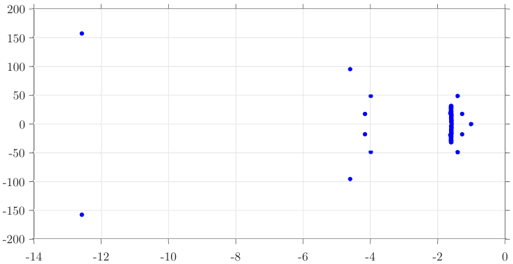
Since the internal model in the controller has dimension $2(2q+1)=42$ , the full size of the controller is $\dim Z=46$ . For simulations we approximate the controlled beam system (1) with a separate higher-dimensional spectral Galerkin approximation with $\dim V_{0}^{N}=69$ . Figure 1 plots some of the eigenvalues of the closed-loop system.

Refer to caption — Figure 1. Eigenvalues of the closed-loop system.

The controller design algorithm in Section 3.2 requires that the system does not have transmission zeros at the (complex) frequencies $\{i\omega_{k}\}_{k=0}^{q}\subset i{\mathbb{R}}$ of the reference and disturbance signals. This property can be tested numerically using the Galerkin approximation of (1) and it is satisfied in our simulations.

The designed internal model based controller is capable of tracking any reference signal $y_{\mbox{\scriptsize{ref}}}(t)$ and any disturbance signal $w_{\mbox{\scriptsize{dist}}}(t)$ of the form (2) with frequencies $(\omega_{k})_{k=0}^{10}$ with arbitrary unknown amplitudes and phases. As explained above, the controller will also approximately track and reject any continuous $2$ -periodic reference and disturbance signals. Figure 2 shows the output $y(t)$ and the tracking error in the case where the first component of $y_{\mbox{\scriptsize{ref}}}(t)$ is a $2$ -periodic triangle signal, the second component of $y_{\mbox{\scriptsize{ref}}}(t)$ is identically zero, and the disturbance signal is $w_{\mbox{\scriptsize{dist}}}(t)=\sin(\pi t)+0.4\cos(3\pi t)$ . The initial deflection $v_{0}(\xi)$ , the initial velocity $v_{1}(\xi)$ and the initial state of the controller are all zero.

Figure 2. The output

y(t)

and the reference signal

y_{\mbox{\scriptsize{ref}}}(t)

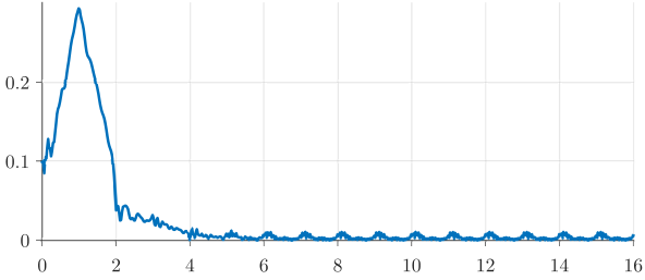
Figure 3 plots the norm of the tracking error $\lVert e(t)\rVert=\lVert y(t)-y_{\mbox{\scriptsize{ref}}}(t)\rVert_{{\mathbb{R}}^{2}}$ . The asymptotic residual error is due to the fact that the internal model contains only a finite number of frequencies and is therefore not capable of tracking the nonsmooth triangle signal with perfect accuracy.

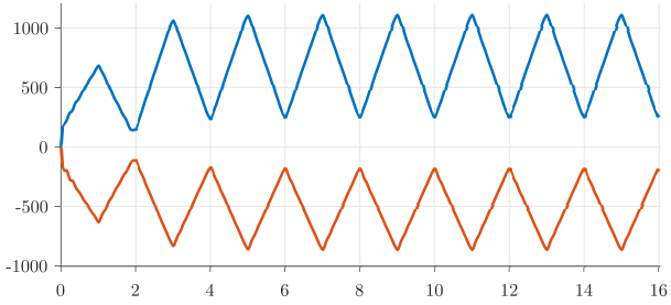
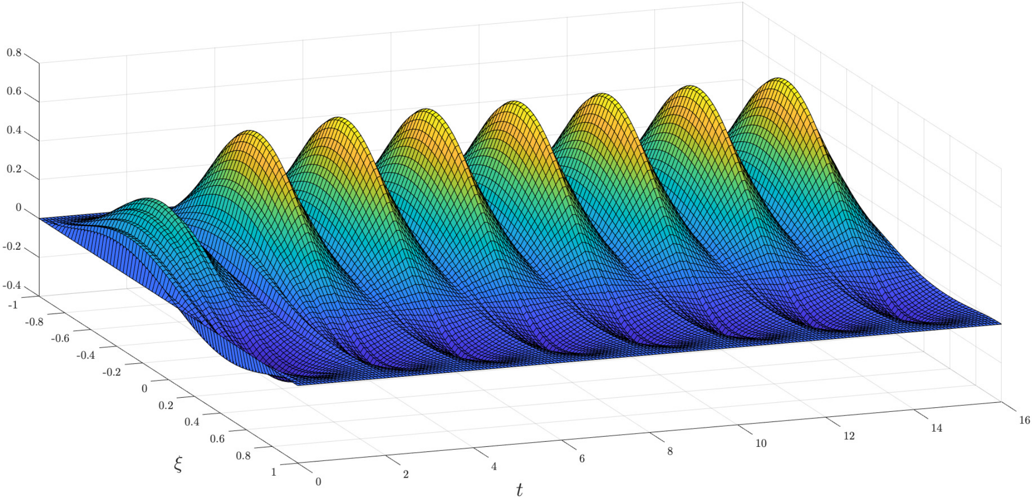
Figure 4 depicts the control actions $u_{1}(t)$ and $u_{2}(t)$ in the simulation. Finally, Figure 5 plots the deflection $v(\xi,t)$ of the controlled beam.

4.1. Comparison with a Low-Gain Controller

Because the beam system is exponentially stable, the output tracking problem can alternatively be solved with a “simple” internal model based controller structure whose dynamics only contain the internal model, i.e.,

	$\displaystyle\dot{z}(t)$	$\displaystyle=G_{1}z(t)+G_{2}e(t),\qquad z(0)\in{\mathbb{R}}^{n_{c}},$
	$\displaystyle u(t)$	$\displaystyle=Kz(t),$

where $G_{1}$ and $G_{2}$ are as in Section 3.2, and thus $n_{c}=2(2q+1)=42$ . As shown in [6, 19] or [15, Rem. 10], the matrix $K\in{\mathbb{R}}^{2\times n_{c}}$ can be chosen as

\displaystyle K

\displaystyle=\varepsilon\bigl[P(0)^{-1},\re P(i\omega_{1})^{-1},\im P(i\omega_{1})^{-1},\ldots,\re P(i\omega_{q})^{-1},\im P(i\omega_{q})^{-1}\bigr],

where $P(\lambda)\in{\mathbb{C}}^{2\times 2}$ is the transfer function of the system (1). For this choice of $K$ , there exists $\varepsilon^{\ast}>0$ such that for any $0<\varepsilon\leq\varepsilon^{\ast}$ the controller achieves output tracking and disturbance rejection for the beam system. In the controller design the values $P(i\omega_{k})$ can be reliably computed using a Galerkin approximation of the system due to the results in [12].

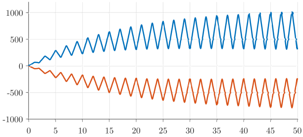
The low-gain parameter $\varepsilon>0$ should be designed so that the closed-loop has the best possible stability margin, and this can be achieved using root locus type analysis. For the beam system (1) with the chosen parameters and the internal model $(G_{1},G_{2})$ with frequencies $\omega_{k}=k\pi$ for $k\in\{0,\ldots,10\}$ , the stabilization of the closed-loop system arising from this controller structure is very difficult due to the high number of unstable frequencies in the internal model. If the number of frequencies is reduced to $\omega_{k}=k\pi$ for $k\in\{0,\ldots,5\}$ (potentially resulting in lower accuracy of the tracking), the best achievable closed-loop stability margin is approximately $0.0382$ with parameter $\varepsilon=0.076$ . The margin can be compared to the stability margin $\approx 1.01$ achieved with the reduced order controller in Section 3.2. This smaller stability margin leads to a significantly slower rate of convergence of the output. Figure 6 depicts the output of the controlled system with the low-gain controller with $\varepsilon=0.076$ .

Figure 6. Output of the system with the low-gain controller.

Note that since in our main controller we were able to choose the size of the reduced order model in Step 4 as $r=4$ , the dimension of our reduced order controller is only higher by $4$ compared to the low-gain controller, but this additional structure of the controller allows the design of a significantly larger stability margin. Since the second controller is based on a low-gain design, it is natural to ask if using this controller leads to reduced control action. However, in the case of a stable linear system with the same number of inputs and outputs the control action required to produce the desired asymptotic output $y_{\mbox{\scriptsize{ref}}}(t)$ does not depend on the type of the internal model based controller (see [16, Lem. 3.10 and proofs of Thm. 3.3 and Lem. 3.4]). Therefore in our simulation the low-gain controller does not achieve output regulation with smaller control gains and the controller requires less control action only for small values of $t\geq 0$ . The control inputs produced by the low-gain controller are depicted in Figure 7.

References

[1] H. T. Banks and K. Ito. Approximation in LQR problems for infinite-dimensional systems with unbounded input operators. J. Math. Systems Estim. Control, 7(1):1–34, 1997.
[2] H. T. Banks and K. Kunisch. The linear regulator problem for parabolic systems. SIAM J. Control Optim., 22(5):684–698, 1984.
[3] C. I. Byrnes, I. G. Laukó, D. S. Gilliam, and V. I. Shubov. Output regulation problem for linear distributed parameter systems. IEEE Trans. Automat. Control, 45(12):2236–2252, 2000.
[4] J. Deutscher. A backstepping approach to the output regulation of boundary controlled parabolic PDEs. Automatica J. IFAC, 57:56–64, 2015.
[5] T. A. Driscoll, N. Hale, and L. N. Trefethen. Chebfun Guide. Pafnuty Publications, 2014.
[6] T. Hämäläinen and S. Pohjolainen. A finite-dimensional robust controller for systems in the CD-algebra. IEEE Trans. Automat. Control, 45(3):421–431, 2000.
[7] E. Immonen. A feedforward-feedback controller for infinite-dimensional systems and regulation of bounded uniformly continuous signals. Internat. J. Robust Nonlinear Control, 16(5):259–280, 2006.
[8] E. Immonen. On the internal model structure for infinite-dimensional systems: Two common controller types and repetitive control. SIAM J. Control Optim., 45(6):2065–2093, 2007.
[9] K. Ito and K. A. Morris. An approximation theory of solutions to operator Riccati equations for $H^{\infty}$ control. SIAM J. Control Optim., 36(1):82–99, 1998.
[10] Feng-Fei Jin and Bao-Zhu Guo. Boundary output tracking for an Euler-Bernoulli beam equation with unmatched perturbations from a known exosystem. Automatica J. IFAC, 109:108507, 9, 2019.
[11] Y. Maday. Analysis of spectral projectors in one-dimensional domains. Math. Comp., 55(192):537–562, 1990.
[12] K. Morris. Design of finite-dimensional controllers for infinite-dimensional systems by approximation. J. Math. Systems Estim. Control, 4(2):1–30, 1994.
[13] V. Natarajan, D. S. Gilliam, and G. Weiss. The state feedback regulator problem for regular linear systems. IEEE Trans. Automat. Control, 59(10):2708–2723, 2014.
[14] L. Paunonen and D. Phan. Reduced order controller design for robust output regulation of parabolic systems. IEEE Trans. Automat. Control, 65(6):2480–2493, 2020.
[15] L. Paunonen. Controller design for robust output regulation of regular linear systems. IEEE Trans. Automat. Control, 61(10):2974–2986, 2016.
[16] L. Paunonen. Robust controllers for regular linear systems with infinite-dimensional exosystems. SIAM J. Control Optim., 55(3):1567–1597, 2017.
[17] L. Paunonen and S. Pohjolainen. Internal model theory for distributed parameter systems. SIAM J. Control Optim., 48(7):4753–4775, 2010.
[18] S. Pohjolainen. A feedforward controller for distributed parameter systems. Internat. J. Control, 34(1):173–184, 1981.
[19] R. Rebarber and G. Weiss. Internal model based tracking and disturbance rejection for stable well-posed systems. Automatica J. IFAC, 39(9):1555–1569, 2003.
[20] Jie Shen. Efficient spectral-Galerkin method II. direct solvers of second- and fourth-order equations using Chebyshev polynomials. SIAM J. Sci. Comput., 16(1):74–87, 1995.
[21] Jie Shen, Tao Tang, and Li-Lian Wang. Spectral methods, volume 41 of Springer Series in Computational Mathematics. Springer, Heidelberg, 2011. Algorithms, analysis and applications.
[22] L. N. Trefethen. Approximation Theory and Approximation Practice. SIAM, Philadelphia, 2013.
[23] Cheng-Zhong Xu and G. Sallet. Multivariable boundary PI control and regulation of a fluid flow system. Math. Control Relat. Fields, 4(4):501–520, 2014.
[24] Xiaodong Xu and S. Dubljevic. Finite-dimensional output feedback regulator for a mono-tubular heat exchanger process. IFAC-PapersOnLine, 49(8):54–59, 2016.