Coarse-grained curvature tensor on polygonal surfaces

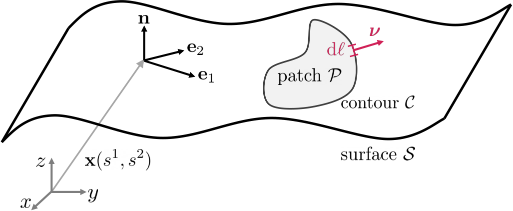
We first consider the case of a smooth surface that can be described using differential geometry. Let $\mathcal{S}$ be a two-dimensional surface parameterized by two coordinates and let $\mathbf{x}(s^{1},s^{2})\in\mathcal{S}$ be a point on this surface. At each point on the surface we associate a local basis composed of two tangent vectors $\mathbf{e}_{1}$ and $\mathbf{e}_{2}$, and a normal vector $\mathbf{n}$, defined as:

see Fig. 1 for illustration. The vectors $\mathbf{e}_{i}$ form the covariant base of the tangent space. We furthermore define the contravariant base $\mathbf{e}^{j}$ as $\mathbf{e}_{i}\cdot\mathbf{e}^{j}=\delta_{i}^{j}$, where $\cdot$ denotes the scalar product, indices run from 1 to 2, and $\delta_{i}^{j}$ is the Kronecker symbol. We also define the local metric tensor with components $g_{ij}=\mathbf{e}_{i}\cdot\mathbf{e}_{j}$ in the local basis $\mathbf{e}_{i}$. Indices can be raised or lowered by contraction with the metric tensor: $a^{i}=g^{ij}a_{j}$ where a summation over repeated indices is implied here and in the following. We denote by $\mathrm{d}\ell$ a line element on the surface with $\mathrm{d}\ell^{2}=g_{ij}\mathrm{d}s^{i}\mathrm{d}s^{j}$, and $\mathrm{d}A=\sqrt{g}\mathrm{d}s^{1}\mathrm{d}s^{2}$ the components of an area element, where $g={\rm det}\,g_{ij}$ is the determinant of the metric tensor. We finally define the local curvature tensor with components $c_{ij}$ given by:

where $\partial_{i}=\partial/\partial s^{i}$. The coordinate-independent form $\bm{c}$ of the curvature tensor is written as:

where $\bm{a}\odot\bm{b}\equiv(\bm{a}\otimes\bm{b}+\bm{b}\otimes\bm{a})/2$ is the symmetric tensor product. The curvature tensor describes changes in the local basis when moving on the surface as described by the Gauss–Weingarten equations Deserno 2004:

where $\nabla_{j}$ denotes the covariant derivative Deserno 2004; Salbreux and Jülicher 2017.

Equation (3) is well-defined for smooth surfaces but difficult to define for surfaces built from discrete components such as particles, molecules, polygons or triangles. We therefore define a coarse-grained curvature measure defined by integrating the curvature tensor over a finite surface patch $\mathcal{P}$. This leads to the definition of the integrated curvature tensor $\bm{M}$:

Using the Gauss–Weingarten equation (4a), the integrand of Eq. (5) can be rewritten as

where the second line has been obtained using Eq. (4b). Then, using the divergence theorem on a curved surface Capovilla and Guven 2002; Salbreux and Jülicher 2017, the integrated curvature tensor is rewritten as a sum of a boundary contribution and a surface term:

Here, $\mathcal{C}$ denotes a contour enclosing the surface patch $\mathcal{P}$, and $\bm{\nu}=\nu_{i}\mathbf{e}^{i}$ is a unit vector, tangent to $\mathcal{P}$, outward-pointing and normal to the contour $\mathcal{C}$ (see Fig. 1).

The definition (6) of the integrated curvature tensor has the form of a sum of two Minkowski tensors. The surface term (first term in Eq. (6)) is proportional to the local three-dimensional Minkowski tensor $W_{2}^{0,2}$ Schröder-Turk et al. 2013. The boundary term (second term in Eq. (6)), is formally a non-Euclidean two-dimensional Minkowski tensor embedded in three-dimensional space. The representation of the integrated curvature tensor given in Eq. (6) reduces for a closed surface $\mathcal{S}$ to a single rank-2 Minkowski tensor $W_{2}^{0,2}=(1/6)\oint_{\mathcal{S}}\mathrm{d}A\,c_{i}^{i}\mathbf{n}\odot\mathbf{n}$ Schröder-Turk et al. 2013, since the contour term vanishes in this case. Importantly, both terms in Eq. (6) are additive and well-defined for a triangulated surface, as we see in the next section.

Furthermore, the integrated mean curvature $M$ over the patch $\mathcal{P}$ can be directly obtained by taking the trace of the integrated curvature tensor defined by Eq. (6):

since ${\rm Tr}\left(\mathbf{e}^{i}\odot\mathbf{n}\right)=0$ and ${\rm Tr}\left(\mathbf{n}\odot\mathbf{n}\right)=1$.

Finally, the integrated curvature tensor can be normalized by the area $A=\int_{\mathcal{P}}\mathrm{d}A$ of patch $\mathcal{P}$ to obtain the coarse-grained curvature tensor $\bm{C}$:

which will be crucial to define a local curvature tensor on polygonal surfaces.

In the following, we consider triangulated surfaces for simplicity. Note that our formalism can be applied to any polygonal surface. The parallel body construction of a triangulated surface, that we describe below, will allow us to define the integrated curvature tensor of surface patches represented by planar triangles and even for a single triangle by using Eq. (6). For this purpose, we first define some notation following Ref. Schröder-Turk et al. 2013. On the triangulated surface, each edge $\mathbf{e}$ is oriented and uniquely assigned to a triangle $T$, and has a counter-oriented edge $\mathbf{e}^{\prime}$ assigned to the adjacent triangle $T^{\prime}$ (see Fig. 2). An oriented edge is also unambiguously assigned to the previous edge $\mathbf{e}_{\rm previous}$ and the next edge $\mathbf{e}_{\rm next}$. This description corresponds to a doubly connected edge list data structure. The normal vector on a triangle $T$ is defined as $\mathbf{n}_{T}=(\mathbf{e}_{\rm previous}\times\mathbf{e})/|\mathbf{e}_{\rm previous}\times\mathbf{e}|$.

The normal vectors $\mathbf{n}_{T}$ and $\mathbf{n}_{T^{\prime}}$ of triangles $T$ and $T^{\prime}$ span the angle $\alpha_{\mathbf{e}}\in(-\pi,\pi]$ at their common edge $\mathbf{e}$. Along each edge $\mathbf{e}$, we define the normalized edge vector $\hat{\mathbf{e}}$, the mean normal vector $\ddot{\mathbf{n}}_{\mathbf{e}}$ and its normal $\dot{\mathbf{n}}_{\mathbf{e}}$, such that

form an orthonormal local basis.

By inflating the triangulated surface by an infinitesimal width $\varepsilon$, we construct a parallel smooth surface that regularizes the sharp edges between triangles by portions of cylinders and portions of spheres which allow the computation of integrated surface quantities (see Fig. 2). We first focus on the computation of the integrated curvature tensor of a single triangle, as the integrated curvature of a patch of triangles is obtained by summing the contribution of individual triangles (see below). The integrated curvature tensor of a single triangle is defined by computing Eq. (6) over the triangle and over the portions of the infinitesimal cylinders that connect it to its neighbors and then by taking the limit $\varepsilon\to 0$. The area contribution appearing in Eq. (6) for a single triangle reads:

where the sum runs over the edges of triangle $T$ and where $\mathbf{n}$ is the normal vector along the portion of cylinder and is parameterized by the angle $\theta$ such that $\mathbf{n}=\cos\theta\,\ddot{\mathbf{n}}_{\mathbf{e}}+\sin\theta\,\dot{\mathbf{n}}_{\mathbf{e}}$ (see App. A and Fig. 8 for details). Note that we integrate over a weighted portion of the cylinder and have therefore introduced the weight fraction $a_{\mathbf{e}}$, which we discuss in the following. Similarly, the boundary contribution is given by:

where $\theta_{\rm f}=\alpha_{\mathbf{e}}(a_{\mathbf{e}}-1/2)$ is the final angle of the portion of cylinder in the local basis defined by Eq. (9), and $\bm{\nu}(\theta_{\rm f})=\mathbf{n}(\theta_{\rm f}+\pi/2)$ $=\hat{\mathbf{e}}\times\mathbf{n}(\theta_{\rm f})$ (see Fig. 8).

Evaluating and summing the contributions from Eqs. (10) and (11), we obtain the integrated curvature tensor $\bm{M}_{T}$ of a single triangle as:

Note that for concave triangles patches, the sign of $\alpha_{\mathbf{e}}$ in Eq. (12) has to be changed (see App. A.3). The weight fraction $a_{\mathbf{e}}$ determines the fraction of the integrated curvature associated with bond $\mathbf{e}$ that is assigned to triangle $T$. Additivity of the integrated curvature tensor imposes $a_{\mathbf{e}}+a_{\mathbf{e}}^{\prime}=1$, where $a_{\mathbf{e}}^{\prime}$ is the weight fraction associated to triangle $T^{\prime}$.

The integrated curvature tensor has the following properties. First, the integrated curvature tensor $\bm{M}$ of a patch $P$ of triangles is directly obtained by summing their individual contributions:

where the sum runs over the triangles $T$ forming patch $P$. Furthermore, similarly to Eq. (7) in the smooth case, the trace of the triangle-based integrated curvature tensor reads:

and corresponds to the weighted sum of the integrated mean curvatures of each edge. Note finally that $\bm{M}_{T}=0$ if the triangle $T$ is surrounded by co-planar triangles (see App. A.2 for details).

The integrated curvature tensor is a cumulative measure of curvature over a surface patch. It is often convenient and useful to define coarse-grained curvature measures, for example to define the curvature on a surface that is formed by discrete particles. Starting from individual triangles, we define the coarse-grained curvature tensor $\bm{C}_{T}$ of triangle $T$ as:

where $A_{T}$ is the area of triangle $T$. Similarly, the coarse-grained curvature tensor for a patch $P$ is given by Eq. (8) with $\bm{M}$ defined in Eq. (13).

If a smooth surface is represented by a triangulation, we demand that the coarse-grained curvature tensor of a triangle converges to the curvature of the smooth surface in the limit where triangles become infinitesimal. This requirement fixes the value of the weight $a_{\mathbf{e}}$ as follows. The coarse-grained mean curvature $H_{T}=\sum_{\mathbf{e}\in T}H_{\mathbf{e}}$ of triangle $T$ combines contributions $H_{\mathbf{e}}=|\mathbf{e}|\alpha_{\mathbf{e}}a_{\mathbf{e}}/(2A_{T})$ from all edges. Convergence to the curvature tensor of a smooth surface requires that the mean curvature associated with a bond is the same for both adjacent triangles $T$ and $T^{\prime}$. Thus, $H_{\mathbf{e}}=H_{\mathbf{e}}^{\prime}$, which together with $a_{\mathbf{e}}+a_{\mathbf{e}}^{\prime}=1$ uniquely determines

Equation (15), together with Eqs. (12) and (16), define the coarse-grained curvature tensor, which is the main result of the paper. This coarse-grained curvature tensor provides a robust definition of curvature on triangulated surfaces, defined for a single triangle and its direct neighbors. The definition (12) of the triangle-based integrated curvature tensor has several appealing properties: (i) owing to the parallel body construction, it is well-defined for triangulated surfaces, (ii) it is additive, and can therefore be used for coarse-graining using Eq. (13), (iii) it displays robust convergence when a triangulation approximates a smooth surface, as we show in the following section.

We have shown that the coarse-grained curvature tensor can be computed for a triangulated surface. We now show that it converges to the curvature tensor of a smooth surface in the limit where the triangle size becomes small. To this end, we consider the curvature tensor of a smooth cylinder, sphere and ellipsoid. For a smooth surface, the curvature tensor (3) is a $3\times 3$ matrix of rank 2, and has three eigenvalues. We denote by $\lambda_{1,2}$ the two principal curvatures, and by $\lambda_{3}=0$ the last eigenvalue, whose eigenvector is parallel to the surface normal. We compare the curvature tensor of smooth surfaces with the coarse-grained curvature tensor $\bm{C}_{T}$ of a single triangle $T$ surrounded by its three direct neighbors with triangle vertices located on the surfaces (see Fig. 3). We determine the coarse-grained curvature tensor of the central triangle using Eqs. (15) and (12) with an area-weight (16). We denote by $\Lambda_{1,2}$ the principal curvatures of the discrete curvature tensor that corresponds to $\lambda_{1,2}$, and by $\Lambda_{3}$ the eigenvalue that converges to 0 and for which the associated eigenvector is parallel to the surface normal as the areas of the triangles become small.

The definition (15) can be used to obtain the local principal directions of the coarse-grained curvature tensor on triangulated surfaces. For this purpose, we have extended the karambola package designed in Ref. Schröder-Turk et al. 2013 to compute the triangle-based curvature tensor on arbitrary surfaces. We provide the corresponding C++ code in App. B. As an illustration, we have determined the principal curvatures and principal directions of curvature of the triangle-based curvature tensor for three examples of closed surfaces with different topology, see Figs. 5, 6 and 7.

Figure 5 displays the principal curvatures and principal directions of curvature for a triangulated Clifford torus. The Clifford torus is an axisymmetric torus with circular cross-section and a ratio $\sqrt{2}$ of the radii of its two generating circles Willmore 1982. It has the important property to minimize $G=\int_{\mathcal{S}}\mathrm{d}A\,(c_{i}^{i})^{2}$ for toroidal topology. We indicate on each triangle the principal directions of the triangle-based curvature tensors as bars with a color which indicates the magnitude of the associated principal curvature. Note that one curvature is constant and positive, while the other is positive (red) on the outer part of the torus and negative (blue) on the inner part of the torus.

From this Clifford torus, we perform a special conformal transformation, which consists of an inversion $\mathbf{R}^{\prime}=\mathbf{R}/R^{2}$, followed by a translation by a vector $\bf t$ and a second inversion, such that a point $\mathbf{R}$ is mapped to Jülicher 1996:

For $\mathbf{t}=1.25r\,\mathbf{e}_{x}$, with $r$ the larger radius of the Clifford torus and $\mathbf{e}_{x}$ a unit vector orthogonal to the axis of symmetry of the torus, the transformation (21) applied to the Clifford torus yields a non-axisymmetric torus with the same minimal value of $G$ (see Fig. 6). Indicated are again the principal curvatures and principal directions of curvature of the triangle-based curvature tensor for each triangle.

The third example, displayed in Fig. 7, is the triangulated Lawson surface of genus 2 Jülicher 1996; Lawson 1970. The Lawson surface minimizes $G$ for genus-2 surfaces. The principal curvatures and principal directions of curvature of the triangle-based curvature tensor are plotted on each triangle. These examples show that the coarse-grained curvature tensor, defined on a triangulation, provides a good approximation for the curvature tensor of the underlying smooth surfaces.

We thank K. Ishihara for bringing Ref. Schröder-Turk et al. 2013 to our attention and for interesting discussions.

References

- Seifert (1997) U. Seifert, “Configurations of fluid membranes and vesicles,” Adv. Phys. 46, 13–137 (1997).
- Bowick and Giomi (2009) M. J. Bowick and L. Giomi, “Two-dimensional matter: Order, curvature and defects,” Adv. Phys. 58, 449–563 (2009).
- Shankar et al. (2020) S. Shankar, A. Souslov, M. J. Bowick, M. C. Marchetti, and V. Vitelli, “Topological active matter,” arXiv:2010.00364 (2020), arXiv:2010.00364 .
- Paulose et al. (2012) J. Paulose, G. A. Vliegenthart, G. Gompper, and D. R. Nelson, “Fluctuating shells under pressure,” Proc. Natl. Acad. Sci. U.S.A. 109, 19551–19556 (2012).
- Mietke et al. (2019) A. Mietke, F. Jülicher, and I. F. Sbalzarini, “Self-organized shape dynamics of active surfaces,” Proc. Natl. Acad. Sci. U.S.A. 116, 29–34 (2019).
- Messal et al. (2019) H. A. Messal, S. Alt, R. M. M. Ferreira, C. Gribben, V. M.-Y. Wang, C. G. Cotoi, G. Salbreux, and A. Behrens, “Tissue curvature and apicobasal mechanical tension imbalance instruct cancer morphogenesis,” Nature 566, 126–130 (2019).
- Helfrich (1973) W. Helfrich, “Elastic Properties of Lipid Bilayers: Theory and Possible Experiments,” Z. Für Naturforschung C 28, 693–703 (1973).
- Helfrich and Prost (1988) W. Helfrich and J. Prost, “Intrinsic bending force in anisotropic membranes made of chiral molecules,” Phys. Rev. A 38, 3065–3068 (1988).
- MacKintosh and Lubensky (1991) F. C. MacKintosh and T. C. Lubensky, “Orientational order, topology, and vesicle shapes,” Phys. Rev. Lett. 67, 1169–1172 (1991).
- Salbreux and Jülicher (2017) G. Salbreux and F. Jülicher, “Mechanics of active surfaces,” Phys. Rev. E 96, 032404 (2017).
- Deserno (2004) M. Deserno, Notes on Differential Geometry (2004).
- Hug (2000) D. Hug, Measures, Curvatures and Currents in Convex Geometry (Albert-Ludwigs-Universität Freiburg, Germany, 2000).
- Schneider and Weil (2008) R. Schneider and W. Weil, Stochastic and Integral Geometry (Springer Science & Business Media, Berlin, Germany, 2008).
- Jensen and Kiderlen (2017) E. B. V. Jensen and M. Kiderlen, eds., Tensor Valuations and Their Applications in Stochastic Geometry and Imaging, Lecture Notes in Mathematics (Springer International Publishing, Cham, 2017).
- Qingde Li and Griffiths (2004) Qingde Li and J. Griffiths, “Least squares ellipsoid specific fitting,” in Geometric Modeling and Processing, 2004. Proceedings (IEEE, Beijing, China, 2004).
- Beale et al. (2016) D. Beale, Y.-L. Yang, N. Campbell, D. Cosker, and P. Hall, “Fitting quadrics with a Bayesian prior,” Comp. Visual Media 2, 107–117 (2016).
- Taubin (1995) G. Taubin, “Estimating the tensor of curvature of a surface from a polyhedral approximation,” Proc. IEEE Comput. Soc. Conf. Comput. Vis. Pattern Recognit. , 902–907 (1995).
- Hameiri and Shimshoni (2003) E. Hameiri and I. Shimshoni, “Estimating the principal curvatures and the darboux frame from real 3-D range data,” IEEE Trans. Syst., Man, Cybern. B 33, 626–637 (2003).
- Ramakrishnan et al. (2010) N. Ramakrishnan, P. B. Sunil Kumar, and J. H. Ipsen, “Monte Carlo simulations of fluid vesicles with in-plane orientational ordering,” Phys. Rev. E 81, 041922 (2010).
- Crane (2020) K. Crane, Discrete Differential Geometry: An Applied Introduction (2020).
- Mecke (2000) K. R. Mecke, “Additivity, Convexity, and Beyond: Applications of Minkowski Functionals in Statistical Physics,” in Statistical Physics and Spatial Statistics (Springer, Berlin, Germany, 2000).
- Schröder-Turk et al. (2013) G. E. Schröder-Turk, W. Mickel, S. C. Kapfer, F. M. Schaller, B. Breidenbach, D. Hug, and K. Mecke, “Minkowski tensors of anisotropic spatial structure,” New J. Phys. 15, 083028 (2013).
- Hadwiger (1951) H. Hadwiger, “Vorlesungen über Integralgeometrie,” Abhdl. Math. Sem. Hamburg 17, 69 (1951).
- Alesker (1999a) S. Alesker, “Description of Continuous Isometry Covariant Valuations on Convex Sets,” Geom. Dedicata 74, 241–248 (1999a).
- Alesker (1999b) S. Alesker, “Continuous Rotation Invariant Valuations on Convex Sets,” Annals of Mathematics 149, 977 (1999b).
- Schneider (2013) R. Schneider, “Local tensor valuations on convex polytopes,” Monatsh. Math. 171, 459–479 (2013).
- Hug and Schneider (2014) D. Hug and R. Schneider, “Local Tensor Valuations,” Geom. Funct. Anal. 24, 1516–1564 (2014).
- Schröder-Turk et al. (2011) G. E. Schröder-Turk, W. Mickel, S. C. Kapfer, M. A. Klatt, F. M. Schaller, M. J. F. Hoffmann, N. Kleppmann, P. Armstrong, A. Inayat, D. Hug, M. Reichelsdorfer, W. Peukert, W. Schwieger, and K. Mecke, “Minkowski Tensor Shape Analysis of Cellular, Granular and Porous Structures,” Adv. Mater. 23, 2535–2553 (2011).
- Bian et al. (2020) X. Bian, S. Litvinov, and P. Koumoutsakos, “Bending models of lipid bilayer membranes: Spontaneous curvature and area-difference elasticity,” Comput. Methods Appl. Mech. Eng. 359, 112758 (2020).
- Jülicher (1996) F. Jülicher, “The Morphology of Vesicles of Higher Topological Genus: Conformal Degeneracy and Conformal Modes,” J. Phys. II France 6, 1797–1824 (1996).
- Beisbart et al. (2006) C. Beisbart, M. S. Barbosa, H. Wagner, and L. d. F. Costa, “Extended morphometric analysis of neuronal cells with Minkowski valuations,” Eur. Phys. J. B 52, 531–546 (2006).
- Beisbart et al. (2002) C. Beisbart, R. Dahlke, K. Mecke, and H. Wagner, “Vector- and Tensor-Valued Descriptors for Spatial Patterns,” in Morphology of Condensed Matter (Springer, Berlin, Germany, 2002).
- Kousholt and Kiderlen (2016) A. Kousholt and M. Kiderlen, “Reconstruction of convex bodies from surface tensors,” Adv. Appl. Math. 76, 1–33 (2016).
- Kousholt (2017) A. Kousholt, “Reconstruction of n-dimensional convex bodies from surface tensors,” Adv. Appl. Math. 83, 115–144 (2017).
- Hansen-Goos and Mecke (2009) H. Hansen-Goos and K. Mecke, “Fundamental Measure Theory for Inhomogeneous Fluids of Nonspherical Hard Particles,” Phys. Rev. Lett. 102, 018302 (2009).
- Hansen-Goos and Mecke (2010) H. Hansen-Goos and K. Mecke, “Tensorial density functional theory for non-spherical hard-body fluids,” J. Phys.: Condens. Matter 22, 364107 (2010).
- Capovilla and Guven (2002) R. Capovilla and J. Guven, “Stresses in lipid membranes,” J. Phys. A 35, 6233–6247 (2002).
- Willmore (1982) T. Willmore, Total Curvature in Riemannian Geometry (Ellis Horwood, Chicester, England, 1982).
- Lawson (1970) H. B. Lawson, “Complete Minimal Surfaces in S 3,” Ann. Math. 92, 335 (1970).
- Lubensky and MacKintosh (1993) T. C. Lubensky and F. C. MacKintosh, “Theory of “Ripple” Phases of Lipid Bilayers,” Phys. Rev. Lett. 71, 1565–1568 (1993).
- Frank and Kardar (2008) J. R. Frank and M. Kardar, “Defects in nematic membranes can buckle into pseudospheres,” Phys. Rev. E 77, 041705 (2008).
- Uchida (2002) N. Uchida, “Dynamics of orientational ordering in fluid membranes,” Phys. Rev. E 66, 040902 (2002).
- Morris and Rao (2019) R. G. Morris and M. Rao, “Active morphogenesis of epithelial monolayers,” Phys. Rev. E 100, 022413 (2019).
- Matoz-Fernandez et al. (2020) D. A. Matoz-Fernandez, F. A. Davidson, N. R. Stanley-Wall, and R. Sknepnek, “Wrinkle patterns in active viscoelastic thin sheets,” Phys. Rev. Research 2, 013165 (2020).
- Merkel et al. (2017) M. Merkel, R. Etournay, M. Popović, G. Salbreux, S. Eaton, and F. Jülicher, “Triangles bridge the scales: Quantifying cellular contributions to tissue deformation,” Phys. Rev. E 95, 032401 (2017).
- Etournay et al. (2015) R. Etournay, M. Popović, M. Merkel, A. Nandi, C. Blasse, B. Aigouy, H. Brandl, G. Myers, G. Salbreux, F. Jülicher, and S. Eaton, “Interplay of cell dynamics and epithelial tension during morphogenesis of the Drosophila pupal wing,” eLife 4, e07090 (2015).