Benford’s laws tests on S&P500 daily closing values and the corresponding daily log-returns
both point to huge non-conformity
Abstract
The so called Benford’s laws are of frequent use in order to observe anomalies and regularities in data sets, in particular, in election results and financial statements. Yet, basic financial market indices have not been much studied, if studied at all, within such a perspective.
This paper presents features in the distributions of S&P500 daily closing values and the corresponding daily log-returns over a long time interval, [03/01/1950 - 22/08/2014], amounting to 16265 data points. We address the frequencies of the first, second, and first two significant digits counts and explore the conformance to Benford’s laws of these distributions at five different (equal size) levels of disaggregation. The log-returns are studied for either positive or negative cases. The results for the S&P500 daily closing values are showing a huge lack of non-conformity, whatever the different levels of disaggregation. Some “first digits” and “first two digits” values are even missing. The causes of this non-conformity are discussed, pointing to the danger in taking Benford’s laws for granted in huge data bases, whence drawing “definite conclusions”. The agreements with Benford’s laws are much better for the log-returns. Such a disparity in agreements finds an explanation in the data set itself: the inherent trend in the index. To further validate this, daily returns have been simulated calibrating the simulations with the observed data averages and tested against Benford’s laws. One finds that not only the trend but also the standard deviation of the distributions are relevant parameters in concluding about conformity with Benford’s laws.
Keywords— S&P500, Benford’s laws, log-returns, closing prices
1 Introduction
[1] noticed that the first few pages of logarithmic table books are more thumbed than the latter ones. He inferred that numbers with smaller initial digits are more often looked for and used than numbers with larger initial digits. Newcomb observation was forgotten for about six decades [2].
In [3], the author apparently and independently11 1 Benford does not cite Newcomb. In fact, neither papers have any bibliography. went much ahead in detail and tested the accuracy of his observation by analyzing a large collection of (in total 20000) numbers, gathered from twenty diverse fields, thereby establishing a law as
| (1) |
for , where is the probability of a number having the first non–zero digit and is the logarithm in base 10.
The first significant digit of a number is its left-most nonzero digit. According to Eq. (1), the smallest digit, 1, should appear as the first digit with the highest proportion (30.1%), whereas the largest digit, 9, will appear as first digit with the least proportion (4.6%).
Thus, , the number of times the integer is observed to be occurring as the first digit, in a data set, is given by the so called “Benford law for the first digit” (BL1 hereafter)
| (2) |
where is the total number of considered data points.
One can show that the probability that is encountered as the second digit is given by “Benford law for the second digit” (BL2 hereafter)
| (3) |
Moreover, one can extend BL1 to the first two digits, a so called BL12,
| (4) |
Following a revival due to Nigrini [4, 5], nowadays, these so called Benford’s laws [6, 7, 2] are of frequent use in order to observe anomalies and regularities in many data sets [e.g. see 8, where widely used survey data sets has been assessed]. In brief, can one trust the data?
Let us warn that Benford’s laws (BLs) unique origin is not accepted by all theoreticians; in fact, it might not be unique. Moreover, some discussion rightly exists on whether Benford’s laws should even be valid at all!. One might also discuss how to test the validity (or not) of BLs [9, 10, 11] and [12] as examples of such considerations, in the field.
Usually, one considers that Benford’s laws should be valid if there is no data manipulation, or if human constraints are non-existent [13]. Yet, there are cases in which Benford laws are either not found to hold, even though their occurrence should be expected [14], or on the contrary are not expected to be observed, but are observed [15, 16, 17, 18, 19, 20]. Thus, testing BLs on various samples should bring some argument about discussing the controversies.
Emphasizing the financial statement aspects, it seems strange to us that basic financial market indices have not been much studied, if studied at all. The section “State of the Art” (Sect. 2) allows us to recall what is presently found in the literature concerning the use of Benford’s laws for studying financial market indices.
In the present paper, we report our study of Benford’s law first, second, and first two digits validity (called BL1, BL2, BL12), upon the S&P500 market closing values, over a long time interval: from 03/01/1950 till 22/08/2014. This amounts to 16265 data points. The time series is downloaded from ‘‘Yahoo! Finance’’, an authoritative web site providing financial data22 2 https://finance.yahoo.com. In doing so we are in line with studies like [21, 22, 23, 20].
We discuss both daily closing values and daily log–returns. Moreover, we divide the whole time interval into five equal size subsets made of 3253 observations each. The interest of such a disaggregation will be explained below.
We observe huge deviations of the market closing values through data histograms with respect to the BLs predictions (or expectations) in Section 3. The findings are in disagreement with [24, 25, 26]. We explain the causes for such a disagreement in Section 5. Concerning the log–returns, it results that the agreement with BLs is much better; we also explain why. The segmentation of the raw data into 5 time intervals is much serving the explanation.
Therefore, even though Benford laws are mainly used to point out to potential frauds in financial statements, by companies [27] or countries [28], one may wonder (or expect) that such << laws >> can be used by investors, or in building pertinent models based on volatility. Beside the findings about data ranges, and the role of digits frequency at some position in the considered numbers, one may suggest further research, pending that the considerations can be tied to other techniques based on the frequency of digits, like letters in a text [29]. This is also relevant to Bayesian approaches (or inputs) and Markov models in investor risk taking aspects.
2 State of the Art
[24] has apparently been the first to examine “the peculiar distribution of the US stock indexes’ digits”. One has to wait 2010, for considerations by Zhao and Wu on the question whether “Chinese stock indices agree with Benford’s Law” [26]. In both cases, [24] and [26], Benford’s law is claimed to be rather valid. Closely connected to our report, [25] checked whether financial markets like the S&P 500 case, from August 14, 1995 to October 17, 2007, thus 3067 data points,obeyed BL1 [25]. The authors also found some reasonable agreement, except, they claim, at anomalous times, like market crashes or special events. Let us mention [30] and [31] where it is tested the “distribution of BIST-100 returns” along BLs. More recently, in 2018, [20] looked at whether BL1 could infer the reliability of financial reports in (6) developing countries. It was shown that “several visually anomalous data have to be a priori removed”, in order to improve the agreement.
Elsewhere, i.e. outside market indices studies, [32] studied LIBOR Manipulation, performing an “Empirical Analysis of Financial Market Benchmarks Using Benford’s Law”. The authors point to “a concentration of notably high deviations from the Benford distribution”. In [33], a decade of financial data for “a large sample of U.S. public companies” is studied along a BL12 perspective. Alali and Romero also broke “down the decade of data into six sub-periods”, and found “different indicators of manipulation”, similar conclusion against Benford’s law compliance are presented in [34] by the same authors.
In so reading, there is no need to say that more analysis can be welcome, and subsequent findings have to be discussed, as it follows here below.
3 Data and data analysis
We have access to the S&P500 daily closing values () via the “Yahoo! Finance” web site. The downloaded data cover a period starting on 03/01/1950 and ending on 22/08/2014; it is reported in USD, see Fig. 1. This amounts to 16265 data points. From such a set, one can easily obtain the 16264 log-returns (); see Fig. 1 also. The main statistical characteristics of such a sample are reported in Table 1. Here it is worth to highlight the huge difference in order of magnitudes for the S&P500 closing values, ranging from at the beginning of the time series to realized in 2014.
Since there is sometimes some discussions on the adequate size of the sample [12] and, for time series, about their “stationarity”, we have also divided the original sample into 5 equivalent size groups; thus each set containing 3253 data points. The corresponding log-returns follow at once.
| S&P500 | ||
|---|---|---|
| Minimum | 16.66 | -0.2290 |
| Maximum | 1992.4 | 0.10957 |
| N. Points | 16265 | 16264 |
| Mean | 451.45 | 2.9403 10-4 |
| Std. Dev. | 514.08 | 9.7315 10-3 |
| Skewness | 1.0637 | -1.0311 |
| Kurtosis | -0.32647 | 27.727 |
A BLs analysis is usually limited to the first, and sometimes second, digit. The second, third and fourth digit distributions are usually found to be rather agreeing with BL2, BL3, and BL4; they can hardly be used for discussion. Sometimes, one finds a study of the first two - BL12 - (and first three digits, BL123). Thus, in order to prepare for a BLs analysis, one usually rounds up the data to at most 5 digits, in order to avoid a rounding of the 4th significant digit if it occurs. We kept that rounding rule even though we only consider the first, second, and first two digits, in order to test BL1, BL2 and BL12 on each S&P500 and log-returns sample. The statistical characteristics of such “adjusted values” are presented in Table 2, for the whole set and for each subsets. The notations seem to be obvious: and , with refer to the subsets. For completeness, let us mention that the upper limits of such subsets are 3253, 6506, 9759, 13012, and 16265, respectively33 3 It can be easily understood that we do not take into account the first value of each log-return subset when dividing the whole set into 5 boxes, in order to have the same number of data points, i.e. 3252 for each subset. This is obviously far from a drastic “assumption”!.


| 16.660 | 1992.4 | 7.34281* | 451.45 | 514.08 | 1.0637 | -0.32647 | |
| 16.660 | 72.640 | 0.13483* | 41.447 | 15.828 | 0.076114 | -1.2629 | |
| 62.070 | 120.24 | 0.29463* | 90.571 | 12.092 | -0.069025 | -0.45554 | |
| 86.900 | 336.77 | 0.51063* | 156.97 | 63.706 | 0.96070 | -0.26424 | |
| 263.82 | 1527.5 | 2.32312* | 714.15 | 389.79 | 0.69803 | -1.0539 | |
| 676.53 | 1992.4 | 4.07961* | 1254.1 | 258.23 | 0.63624 | 0.30357 | |
| -0.22900 | 0.10957 | 4.7821 | 2.9403** | 97.315** | -1.0311 | 27.727 | |
| -0.06909 | 0.04544 | 1.32420 | 4.0721** | 74.371** | -0.71995 | 8.1493 | |
| -0.03740 | 0.04900 | 0.35396 | 1.0884** | 76.573** | 0.22745 | 3.3794 | |
| -0.22900 | 0.08709 | 1.13920 | 3.5031** | 101.43** | -3.6266 | 84.952 | |
| -0.07113 | 0.04989 | 1.26110 | 3.8778** | 96.784** | -0.35884 | 4.8634 | |
| -0.09470 | 0.10957 | 0.72213 | 2.2206** | 127.70** | -0.21277 | 9.1859 |
One can observe much variety in the data reported in Table 2: for example, there are large negative log-returns due to a few crashes, whence the standard deviation can also be very high. Also, the skewness and kurtosis, either for the S&P500 raw data and for the log-returns have different orders of magnitude.
Thereafter, we can compare the number of first, second, and first two digits in such data sets (12, 5 for closing prices, 5 for log-returns and 2 for the global analysis). In the nomenclatures, we distinguish the 5 subsets by different symbols.
Two warnings first: (i) officially, a zero cannot be a first digit, when studying BLs; (ii) decimal points separators are also ignored. Nevertheless, in our counting algorithms, we have kept 0 as a bona fide first (and also second) digit in the case of BLs tests on the log-returns. Indeed, in several (124) cases, these log-returns are strictly equal to 0, because there was no change in two successive S&P500 closing values. In such cases, the second digit is of course also 0. Keeping such a digit, for the tests on log-returns, allows one to observe the “relative importance” of such events; obviously . It is easily admitted that the importance is “not great”. However, “necessarily”, the number of observed events, , with , thereafter differs in the previously imposed equal size intervals because the zeros are not homogeneously distributed across the 5 log-return subsets.
Here, we want at once to emphasize the following: some “first digits”, whence “first two digits”, values are missing in various subsets. For example, the missing first digits in each , can be found from Table 3; this is also clearly observed in the first digit figure for S&P500, Fig. 2, where one has stacked up the subset histograms.
| 1 | 2 | 3 | 4 | 5 | 6 | 7 | 8 | 9 | |
|---|---|---|---|---|---|---|---|---|---|
| 234 | 898 | 252 | 812 | 689 | 299 | 69 | 0 | 0 | |
| 735 | 0 | 0 | 0 | 0 | 185 | 427 | 921 | 985 | |
| 2026 | 650 | 93 | 0 | 0 | 0 | 0 | 58 | 426 | |
| 899 | 117 | 682 | 818 | 171 | 220 | 126 | 60 | 160 | |
| 2751 | 0 | 0 | 0 | 0 | 4 | 27 | 229 | 242 |
This is not a trivial point; one understands (a posteriori) that this is due to the presence of different trends in the data; see the discussion in Sect. 5 .
Fig. 2 presents the data for testing BL1 on the whole S&P500 daily closing values and on the corresponding log-returns. The divisions by colour provides information about the examined time intervals. Fig. 3 presents the corresponding BL2 data, and Fig. 4 the data serving for a BL12 analysis. At once, visually, the S&P500 data looks hardly representable by a log function, like Eqs.(2)-(4). In contrast, the log-returns histograms have a more appealing form. Notice that we distinguish negative and positive log-returns, and mention on each graph the occurrence of strictly zero and double zero values.
In Table 4, we report the test of variables conformity with BL1, BL2, and BL12 for the S&P500 whole data set and for the subsets; the number of observations (or data points) is indicated for each case: 16265 and, for the five subsets, 3253 data points, respectively. The number of degrees of freedom (), easily derived from the number of bins, is also indicated with the “critical” value. One can hardly admit any conformity, given the large values compared to the “critical” value. Even if a test can be claimed as not being the most powerful test for BL conformance [10], the current results are so different from “any good expectation” that the utilization of another test will be unlikely able to inverse the conclusions.
| BL1 | BL2 | BL12 | ||
|---|---|---|---|---|
| : | 8 | 9 | 89 | |
| : | 15.507 | 16.919 | 112.022 | |
| 16265 | 3756.03 | 397.46 | 7084.40 | |
| 3253 | 2737.22 | 387.46 | 5030.895 | |
| 3253 | 10038.14 | 544.12 | 12840.86 | |
| 3253 | 2936.91 | 527.02 | 5561.862 | |
| 3253 | 1476.73 | 302.02 | 3496.052 | |
| 3253 | 5187.90 | 813.99 | 7664.894 |
| BL1 | BL2 | BL12 | ||
| : | 8 | 9 | 89 | |
| 15.507 | 16.919 | 112.022 | ||
| 16140 | ||||
| 16136 | 156.66 | 4.18 | 255.96 | |
| 3174 | 101.34 | 10.88 | 213.45 | |
| 3226 | 16.61 | 16.30 | 146.46 | |
| 3237 | 86.25 | 8.31 | 172.70 | |
| 3249 | 33.99 | 4.49 | 101.39 | |
| 3250 | 19.11 | 5.42 | 102.23 | |
| 8616 | ||||
| 8614 | 115.06 | 4.73 | 198.02 | |
| 1742 | 74.97 | 5.41 | 168.53 | |
| 1687 | 28.58 | 21.38 | 135.47 | |
| 1690 | 33.30 | 5.87 | 108.90 | |
| 1726 | 26.24 | 5.42 | 113.55 | |
| 1769 | 17.04 | 7.52 | 91.69 | |
| 7524 | ||||
| 7522 | 54.46 | 7.01 | 164.81 | |
| 1432 | 34.07 | 10.24 | 145.76 | |
| 1539 | 5.59 | 9.53 | 120.75 | |
| 1547 | 59.53 | 8.06 | 154.73 | |
| 1523 | 15.37 | 5.30 | 83.38 | |
| 1481 | 12.56 | 13.98 | 123.31 | |
Let us turn our attention to the log-returns. As mentioned, there are 124 cases in which the log-return is equal to 0, since the closing prices are identical two consecutive days; these cases occur unevenly in the different intervals: for completeness, let us mention their occurrence: 78, 26, 15, 3, and 2 times, respectively. This influences the number of observations in each subgroup; see first column in Table 5.
Therefore, there are 16264 - 124 = 16140 cases to be examined in the whole series. When dividing the series into 5 subsets, for coherence, the first value in the , subsets are disregarded, since the first one (day) is “missing” in the case. Thus the number of observations on which to test BL1 amounts to 16260 - 124 = 16136.
The number of data points should be expected to be 3252 for the five subsets. However, , the number of observations in the -subset, varies in each subset, since one is not taking into account the number (124) of log-return values strictly equal to 0, and such a number is not uniformly distributed through the subsets. Moreover, notice that we distinguish (top of Table 5) the case of the absolute values of log-returns and those corresponding to either positive or negative log-return sign (two bottom sub-tables).
The results of the test of variables conformity with BL1, BL2, and BL12 for the S&P500 corresponding daily log-returns () for the whole data set and for the subsets are given in Table 5. BL1 is hardly obeyed, but the difference between the values and the is not so big as for the closing prices sample. Some exceptional cases appear to obey BL1, all of the fall in the study of negative returns, , and . The situation is almost perfect for BL2, for which only is slightly disagreeing. In the case of BL12, only the latest subsets present some agreement, but the first subset and the whole sample series are surely not obeying BL12.
Our explanation follows in the conclusion section.
4 A Benford Law compliant price paths generator?
To stress the dependence from the distributional features of the data against the numerousness of the observations, we test the ability of the standard Geometric Brownian Motion (GBM), [35], in producing a Benford Law compliant series of returns.
Along the standard GBM formulation, one has
| (5) |
where is the log-returns, is the mean and is the standard deviation of the log-returns, is the time and is the Wiener process or Brownian motion. Assuming log-normally distributed returns, calibrating the mean via the empirical observations, we aim at finding the level of that makes the returns simulated via the GBM as close as possible to the BL1, BL2, BL12 compliance, employing 2 criteria later described.
In so doing we have simulated the returns via the following relationship:
| (6) |
where has been set equal to 1 for convenience without harming the relationship, is the average of the returns for the cases , is the standard deviation from the array ranging from 0.0001 to 0.5 with a step of 0.0001 (the range is set to embed the standard deviations reported in Table 2). is an array made of 5000 random extractions from a . Thus, contains 5000 simulated returns with average for each and each . Therefore, per each of we have a matrix with 5000 rows (simulated days) and 5000 columns (one per each ).
From now on, indicates the standard deviation which produced the most compliant BL price path for the respective . Therefore, for each column of , we calculate the chi-square statistic against the BL theoretical values for BL1, BL2 and BL12 [36, 37, in doing so we are in line with the usage of the test in comparing disitrubutions, see]. We have determined the target levels by using the following 2 criteria separately:
- A.
Minimum euclidean distance between the threshold levels of the chi-square distribution at 5% significance (considering the respective degrees of freedom, see Table 5) and the observed chi-square levels. The relationship employed is:
(7) Where, representing respectively the stance for first, second and first two digits, are the observed chi-square statistics and is the pointer addressing the level of ; are the threshold taken for the case of significance. For each vector, the is reported in Table 6.
- B.
For both criteria used, the results clearly prove that the standard GBM used for simulating returns makes it impossible to get a joint compliance with BL1, BL2 and BL12 when starting from the mean calibrated on real data. Furthermore, even using 5000 simulated daily returns, one cannot reach satisfactory results.
A closer look at the results lead to additional comments. Under the criterion A (see Table 6), the returns simulated with the mean of leads to a = 0.0865 which is very close to the observed standard deviation for , namely 0.0101. However, the tests fail for all the digits apart the second, as per the real data (see Table 5); in addition, the second digits presents a remarkably low statistics. The other s are meaningless ; namely they give values rarely met in a financial Market ; the statistics do not present a relationship with the sensibleness of the estimations.
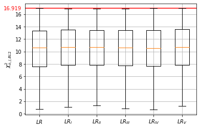
The outcomes resulting from the criterion B confirm that the second digits are the most BL compliant. Table 7 shows the number of cases for which the chi-square statistics pass the test with 5% significance; it happens in more than 70% of the cases for each stance, namely for the majority of the plugged in Eq. (6). Fig. 6a hints about the distributions of the statistics whose frequencies are reported in Table 7. The obtained when applying the criterion B are summarized in Table 8 and showed in Fig. 6b. Most of them are pretty high as testified by the mean and the standard deviation reported in the summary statistics and in the box.
Summarizing, the results show sensitivity to and to the presence of trends in the data. Besides, the behaviors are different, therefore, per each digit studied against the respective Benford’s law, dedicated consideration should be run before grasping conclusions on the data.
| BL1 | BL2 | BL12 | |||
|---|---|---|---|---|---|
| : | 8 | 9 | 89 | ||
| 15.507 | 16.919 | 112.022 | |||
| eucl. dist. | BL1 | BL2 | BL12 | ||
| 0.2561 | 210.30 | 159.29 | 12.17 | 265.42 | |
| 0.2428 | 205.41 | 163.80 | 5.39 | 253.69 | |
| 0.2318 | 201.60 | 157.44 | 10.01 | 255.02 | |
| 0.0865 | 204.60 | 127.21 | 6.89 | 283.15 | |
| 0.2081 | 195.18 | 152.88 | 13.01 | 250.63 | |
| 0.2382 | 193.53 | 158.17 | 7.72 | 242.47 | |
| BL1 | BL2 | BL12 | |
|---|---|---|---|
| : | 8 | 9 | 89 |
| 15.507 | 16.919 | 112.022 | |
| 0 | 3596 | 0 | |
| 0 | 3610 | 0 | |
| 0 | 3639 | 0 | |
| 0 | 3619 | 0 | |
| 0 | 3640 | 0 | |
| 0 | 3576 | 0 |
| 0.2417 | 0.1441 | 1.6778 | |
| 0.2423 | 0.1435 | 1.6886 | |
| 0.2419 | 0.1450 | 1.6688 | |
| 0.2427 | 0.1431 | 1.6967 | |
| 0.2418 | 0.1436 | 1.6837 | |
| 0.2420 | 0.1442 | 1.6786 |
5 Conclusions
In view of increasing knowledge about applications of Benford’s laws, we have analyzed features in the distributions of S&P500 daily closing values and the corresponding daily log-returns over a long time interval, that is, from the first days of January 1950 till almost the end of August 2014, amounting to 16265 data points. We have addressed our considerations to the amount of first, second and first two significant digits. We have also explored the conformance to Benford’s laws of these distributions distinguishing five different (equal size) levels of disaggregation, in order to test some (non)stationarity (hidden) feature, - if it might occur. Moreover, although this is not usual, we have distinguished negative log-returns from positive ones, plus their combination, since we have enough available data points.
The results for the S&P500 daily closing values () are unexpectedly showing a huge lack of conformity, whatever the different levels of disaggregation. We have noticed that some “first digits” and “first two digits” values are missing in some subsets. The agreements with Benford’s laws are much better for the log-returns (). Such a disparity in agreements finds an explanation in the data set itself, rather than in a possibility of fraud!
In fact, this feature allows us to comment on some often forgotten criterion for testing the conformity of BLs [12]. Indeed, one should emphasize that BLs could only be usefully studied and observed if all digits - from 1 to 9 - are well represented as every first digit. A time series or a set of data points should first be tested for its range, basically, the minimum and maximum values. The argument is here well sustained by observing the evolution of the S&P500 over time.
Fig. 5 provides a semi-log view of the S&P500 closing values; the five studied subsets are emphasized. This allows one to understand why the distributions of digits are peculiar. Having “abandoned” a 1 first digit in some sector due to the financial trend, it takes “a while” before one goes from a 9 to a new 1 (for the following decade for example). Another example showing why sometimes a BL analysis and anomaly deduction might be doubtful is found in sector : the index starts from 62, reaches 89, but never goes to any 50, or 20 or 200, a fortiori 300, etc. Thus, the index “misses” a few first digit values. The same observation goes true for the other sectors where first digits are missing. In the present analysis of a financial market, this is due to the inherent trend in the index. Such causes for no conformity explains previously puzzling observations like in [15]. Related explanations do follow for cases of data containing crashes, and “long time” spent in growing and recovering [25].
Thus, beside a thorough analysis of a financial index, a case rarely examined, surely over a so big set of data points, specific causes of this non-conformity are presented, pointing to the danger of taking Benford’s laws for granted in huge data bases, whence leading to “definite conclusions”.
One often reads “the more, the better” as in [38] or [39] where it is claimed “the larger, the better” for applying Benford’s laws and deducing fraud or not through lack of conformity or not. This is not true! A large set of data points is neither a sufficient nor necessary criterion for such a statistical conformity test [40]. Under this perspective, we have simulated 5000 daily returns using the averages of the real data presented in Section 3 with the Geometric Brownian Motion formulation, see Eq.(6). In addition, for each mean, hence for each studied time span, the standard deviations plugged in Eq.(6) range in [0.0001 - 0.5] (with steps of 0.0001). The BL compliance results are in line with the outcomes obtained with the observed data. This is an additional hint; in fact, one needs to consider the distributional features of the phenomenon under investigation instead of only focusing on the number of observations or on the granularity of the data. This type of comments is in line with [41], where the author has commented comparable exercise runs for studying fraud detection application of BL in political elections.
Finally, recall that BLs are used to detect fraud mainly. Of course, there are data sets which can be hardly manipulated. We are all convinced that S&P 500 and other financial indices result from averages, thus apparently obeying the BL validity theoretical criteria, whence could not have fraudulent aspects. However, the present study suggests that one might use BLs at a more << microscopic level >>, that of company share price, as already appreciated by [27].
As already stated, one of the main findings of our research has been about the data range. Indeed to conform with the law, the data set must contain data in which each number 1 through 9 has an equal chance of being the leading digit; there should be equipartition [42, 43]. However, this seems paradoxical. What we show is that the data transformation, from the raw index value to the log-return space, is a key step for observing that there is no data manipulation and obedience to BL. The trend value is avoided. Moreover, BL2 and BL12 are less sensitive to trend manipulation.
As so observed, one may imagine that BL2 and BL12 are of interest for investors, since a change of the first digit is rather rare when share prices are higher than 10 (whatever the currency is in fact). BL1 should be verified for << cheap prices >>, lower than 10. This would lead to an investment strategy similar to that considering the equivalence of digits in data series to letters in texts [44]. Whence it would be interesting for financial analysts to reconsider a connection between Benford and Zipf law approaches.

References
- [1] S. Newcomb, “Note on the frequency of use of the different digits in natural numbers,” American Journal of Mathematics, vol. 4, no. 1, pp. 39–40, 1881.
- [2] T. A. Mir and M. Ausloos, “Benford’s law: A “sleeping beauty" sleeping in the dirty pages of logarithmic tables.,” Journal of the Association for Information Science and Technology, vol. 69, no. 3, pp. 349–358, 2018.
- [3] F. Benford, “The law of anomalous numbers,” Proceedings of the American Philosophical Society, vol. 78, no. 1, pp. 551–572, 1938.
- [4] M. J. Nigrini, “A taxpayer compliance application of Benford’s law,” The Journal of the American Taxation Association, vol. 18, no. 1, pp. 72–91, 1996.
- [5] M. J. Nigrini and L. J. Mittermaier, “The use of Benford’s law as an aid in analytical procedures,” Auditing: A Journal of Practice & Theory, vol. 16, no. 2, pp. 52–67, 1997.
- [6] A. Berger and T. P. Hill, An introduction to Benford’s law. Princeton University Press, 2015.
- [7] S. J. Miller, Benford’s Law: Theory and Applications. Princeton University Press, 2015.
- [8] M. Kaiser, “Benford’s law as an indicator of survey reliability– can we trust our data?,” Journal of Economic Surveys, vol. 33, no. 5, pp. 1602–1618, 2019.
- [9] G. D’Amico, “A semi-Markov approach to the stock valuation problem,” Annals of Finance, vol. 9, no. 4, pp. 589–610, 2013.
- [10] M. Lesperance, W. Reed, M. Stephens, C. Tsao, and B. Wilton, “Assessing conformance with Benford’s law: Goodness-of-fit tests and simultaneous confidence intervals,” PloS one, vol. 11, no. 3, p. e0151235, 2016.
- [11] N. Omerzu and I. Kolar, “Do the Financial Statements of Listed Companies on the Ljubljana Stock Exchange Pass the Benford’s Law Test?,” International Business Research, vol. 12, no. 1, pp. 54–64, 2019.
- [12] A. Berger and T. P. Hill, “The mathematics of Benford’s law: a primer,” Statistical Methods & Applications, vol. 1, pp. 1–17, 2020.
- [13] U. Hassler and M. Hosseinkouchack, “Testing the Newcomb-Benford law: experimental evidence,” Applied Economics Letters, vol. 26, no. 21, pp. 1762–1769, 2019.
- [14] M. Ausloos, C. Herteliu, and B. Ileanu, “Breakdown of Benford’s law for birth data,” Physica A: Statistical Mechanics and its Applications, vol. 419, pp. 736–745, 2015.
- [15] P. Clippe and M. Ausloos, “Benford’s law and Theil transform of financial data,” Physica A: Statistical Mechanics and its Applications, vol. 391, no. 24, pp. 6556–6567, 2012.
- [16] T. A. Mir, M. Ausloos, and R. Cerqueti, “Benford’s law predicted digit distribution of aggregated income taxes: the surprising conformity of Italian cities and regions,” The European Physical Journal B, vol. 87, no. 11, p. 261, 2014.
- [17] R. Cerqueti and M. Ausloos, “Evidence of economic regularities and disparities of Italian regions from aggregated tax income size data,” Physica A: Statistical Mechanics and its Applications, vol. 421, pp. 187–207, 2015.
- [18] T. A. Mir, “The leading digit distribution of the worldwide illicit financial flows,” Quality & Quantity, vol. 50, no. 1, pp. 271–281, 2016.
- [19] M. Ausloos, R. Cerqueti, and T. A. Mir, “Data science for assessing possible tax income manipulation: The case of Italy,” Chaos, Solitons & Fractals, vol. 104, pp. 238–256, 2017.
- [20] J. Shi, M. Ausloos, and T. Zhu, “Benford’s law first significant digit and distribution distances for testing the reliability of financial reports in developing countries,” Physica A: Statistical Mechanics and its Applications, vol. 492, pp. 878–888, 2018.
- [21] J. L. Juergens and L. Lindsey, “Getting out early: an analysis of market making activity at the recommending analyst’s firm,” The Journal of Finance, vol. 64, no. 5, pp. 2327–2359, 2009.
- [22] M. R. Haley, “K-fold cross validation performance comparisons of six naive portfolio selection rules: how naive can you be and still have successful out-of-sample portfolio performance?,” Annals of Finance, vol. 13, no. 3, pp. 341–353, 2017.
- [23] J. Riccioni and R. Cerqueti, “Regular paths in financial markets: Investigating the Benford’s law,” Chaos, Solitons & Fractals, vol. 107, pp. 186–194, 2018.
- [24] E. Ley, “On the peculiar distribution of the US stock indexes’ digits,” The American Statistician, vol. 50, no. 4, pp. 311–313, 1996.
- [25] M. Corazza, A. Ellero, and A. Zorzi, “Checking financial markets via Benford’s law: the S&P 500 case,” in Mathematical and statistical methods for actuarial sciences and finance, pp. 93–102, Springer, 2010.
- [26] S. Zhao and W. Wu, “Does Chinese Stock Indices Agree with Benford’s Law?,” in 2010 International Conference on Management and Service Science, pp. 1–3, IEEE, 2010.
- [27] A. D. Saville, “Using Benford’s law to detect data error and fraud: an examination of companies listed on the Johannesburg Stock Exchange: economics,” South African Journal of Economic and Management Sciences, vol. 9, no. 3, pp. 341–354, 2006.
- [28] B. Rauch, M. Göttsche, G. Brähler, and S. Engel, “Fact and fiction in EU-governmental economic data,” German Economic Review, vol. 12, no. 3, pp. 243–255, 2011.
- [29] E. Shulzinger and E. Bormashenko, “On the universal quantitative pattern of the distribution of initial characters in general dictionaries: The exponential distribution is valid for various languages,” Journal of Quantitative Linguistics, vol. 24, no. 4, pp. 273–288, 2017.
- [30] M. Cinko, “Testing distribution of BIST-100 returns by Benford Law,” Journal of Economics Finance and Accounting, vol. 1, no. 3, pp. 184–191, 2014.
- [31] A. Aybars and L. Ataunal, “An Application of Benford’s Law to Fundamental Accounting Figures Reported by Borsa Istanbul (BIST) Companies.,” Journal of Economics Finance and Accounting, vol. 3, no. 3, pp. 234–243, 2016.
- [32] B. Rauch, M. Goettsche, and F. El Mouaaouy, “LIBOR Manipulation–Empirical Analysis of Financial Market Benchmarks Using Benford’s Law,” Available at SSRN 2363895, 2013.
- [33] F. A. Alali and S. Romero, “Benford’s Law: Analyzing a decade of financial data,” Journal of Emerging Technologies in Accounting, vol. 10, no. 1, pp. 1–39, 2013.
- [34] F. Alali and S. Romero, “Characteristics of failed us commercial banks: an exploratory study,” Accounting & Finance, vol. 53, no. 4, pp. 1149–1174, 2013.
- [35] A. Einstein, “Über die von der molekularkinetischen theorie der wärme geforderte bewegung von in ruhenden flüssigkeiten suspendierten teilchen,” Annalen Der Physik, vol. 4, pp. 549–560, 1905.
- [36] A. L. Christensen and R. M. Mohr, “Nonprofit lobbying: Museums and collections capitalization,” Financial Accountability & Management, vol. 15, no. 2, pp. 115–133, 1999.
- [37] T. Dissanayake, S. Dellaportas, and P. W. S. Yapa, “The diffusion-adoption of accrual accounting in Sri Lankan local governments,” Financial Accountability & Management, vol. 36, no. 3, pp. 261–277, 2020.
- [38] G. Nairn, “Beating fraudsters at their own game.” www.geoffnairn.com/wordpress/?p=726, 2011. Online; accessed 23-September-2019.
- [39] J. C. Collins, “Using Excel and Benford’s Law to Detect Fraud: Learn the Formulas, Functions, and Techniques That Enable Efficient Benford Analysis of Data Sets,” Journal of Accountancy, vol. 223, no. 4, p. 44, 2017.
- [40] F. Heilig and E. J. Lusk, “Testing the Small Size Effect Bias for Benford Screening: The False Negative Signaling Error,” Business Management Dynamics, vol. 8, no. 6, p. 23, 2018.
- [41] W. R. Mebane, “Comment on “Benford’s Law and the detection of election fraud”,” Political Analysis, vol. 19, no. 3, pp. 269–272, 2011.
- [42] É. Janvresse and T. De la Rue, “From uniform distributions to Benford’s law,” Journal of Applied Probability, vol. 41, no. 4, pp. 1203–1210, 2004.
- [43] J. R. Iafrate, S. J. Miller, and F. W. Strauch, “Equipartitions and a distribution for numbers: A statistical model for Benford’s law,” Physical Review E, vol. 91, no. 6, p. 062138, 2015.
- [44] M. Ausloos and P. Bronlet, “Strategy for investments from Zipf law(s),” Physica A: Statistical Mechanics and its Applications, vol. 324, no. 1-2, pp. 30–37, 2003.