SALT3: An Improved Type Ia Supernova Model for Measuring Cosmic DistancesAstroPy (Astropy Collaboration et al. 2013; Astropy Collaboration et al. 2018),Astroquery (Ginsburg et al. 2019),extinction(Barbary 2016),iMinuit (James & Roos 1975; Dembinski et al. 2020), Matplotlib (Hunter 2007), NumPy (Harris et al. 2020),SciPy (Virtanen et al. 2020), sncosmo (Barbary et al. 2015; Barbary et al. 2016), tqdm (da Costa-Luis et al. 2021)
Abstract
A spectral-energy distribution (SED) model for Type Ia supernovae (SNe Ia) is a critical tool for measuring precise and accurate distances across a large redshift range and constraining cosmological parameters. We present an improved model framework, SALT3, which has several advantages over current models including the leading SALT2 model (SALT2.4). While SALT3 has a similar philosophy, it differs from SALT2 by having improved estimation of uncertainties, better separation of color and light-curve stretch, and a publicly available training code. We present the application of our training method on a cross-calibrated compilation of 1083 SNe with 1207 spectra. Our compilation is larger than the SALT2 training sample and has greatly reduced calibration uncertainties. The resulting trained SALT3.K21 model has an extended wavelength range - Å (1800 Å redder) and reduced uncertainties compared to SALT2, enabling accurate use of low- and photometric bands. Including these previously discarded bands, SALT3.K21 reduces the Hubble scatter of the low-z Foundation and CfA3 samples by 15% and 10%, respectively. To check for potential systematic uncertainties we compare distances of low () and high () redshift SNe in the training compilation, finding an insignificant mmag shift between SALT2.4 and SALT3.K21. While the SALT3.K21 model was trained on optical data, our method can be used to build a model for rest-frame NIR samples from the Roman Space Telescope. Our open-source training code, public training data, model, and documentation are available at https://saltshaker.readthedocs.io/en/latest/, and the model is integrated into the sncosmo and SNANA software packages.
I Introduction
Type Ia supernovae (SNe Ia) have been used as cosmological distance indicators for more than two decades, providing early evidence of the accelerating expansion of the Universe (Riess et al. 1998; Perlmutter et al. 1999). Today, SN Ia distances are used at low redshift () for distance ladder measurements of the Hubble constant (Riess et al. 2021; Freedman et al. 2019, H0;), currently the subject of a tension (see Verde et al. 2019 for a review), as well as measurements of the dark energy equation-of-state parameter, which incorporate SNe at (currently consistent with ; Scolnic et al. 2018; Abbott et al. 2019; Jones et al. 2019). Recent measurements of (Riess et al. 2016), as well as most large studies of SNe across the observed redshift range for the last decade (Guy et al. 2010; Conley et al. 2011; Sako et al. 2018; Betoule et al. 2014; Riess et al. 2018; Scolnic et al. 2018; Brout et al. 2019a; Jones et al. 2019), have relied upon the SALT2 light-curve model (Guy et al. 2007; Guy et al. 2010) for the brightness standardization of SNe Ia in their analysis.
SN Ia distances are typically estimated by fitting their light curves with a model to determine an overall flux, a color, and one (or more) light-curve shape parameters. The apparent magnitude (as computed from the flux) is standardized with a linear combination of color and light-curve parameters (referred to as the Tripp estimator; Tripp 1998) to produce a standardized apparent magnitude relative to a fiducial SN Ia. The SALT2 ( Spectral Adaptive Light-curve Template) model describes SN Ia light curves as a combination of component spectral energy distributions (flux surfaces defined in wavelength and time), multiplied by a color-dependent term described by a color law that is similar to that of the Milky Way. These components are determined through a ‘‘model training’’ process; the last trained model to be used in a published cosmological analysis was SALT2.4 (which we hereafter refer to as SALT2.JLA11 1 JLA refers to ”Joint Lightcurve Analysis” that included the SDSS-SN and SNLS teams, and produced cosmology results in Betoule et al. 2014 ), presented in Betoule et al. 2014 and Mosher et al. 2014, although a retrained model has recently been presented in Taylor et al. 2021. The ubiquity of the SALT2 model in cosmology analyses of the last decade can be attributed to:
- 1.
The spectrophotometric model can be integrated over filter bands using the appropriate rest-frame wavelengths, which removes the need for explicit -corrections.
- 2.
The training process is cosmology independent, as the overall normalization of a light curve is a fitted parameter.
- 3.
The training set incorporates photometric data from multiple surveys, reducing the sensitivity of the model to the calibration of any one survey.
- 4.
The training sample incorporates high redshift photometric data, allowing the use of well-calibrated observer-frame optical data to extend the model into the rest-frame ultra-violet (UV).
- 5.
Publicly available analysis tools such as SNANA (Kessler et al. 2009b) and sncosmo. (Barbary et al. 2015; Barbary et al. 2016) include infrastructure to fit lightcurves and generate simulated data using the SALT2 model.
- 6.
The model has been tested by many independent groups as a consequence of its use in cosmology analyses.
Despite these advantages, Scolnic et al. 2018 found that the calibration of the training sample used to create the SALT2.JLA model was the largest single systematic uncertainty in their measurement of (, 30% of the total systematic uncertainty), though a new analysis methodology could somewhat reduce this uncertainty (Brout et al. 2020). Achieving the science goals of the Vera C. Rubin Observatory’s Legacy Survey of Space and Time (LSST) will require that systematic uncertainty in the calibration of the light-curve model be decreased by a factor of 5 for the year-one analysis (The LSST Dark Energy Science Collaboration et al. 2018).
The SALT2.JLA model does not fully reproduce observed spectral features such as varying absorption line velocities (Foley & Kasen 2011; Siebert et al. 2020). Similarly, studies have found evidence that standardized distances based on SALT2 with the Tripp estimator (SALT2+Tripp) are dependent on SN Ia host galaxy properties (Kelly et al. 2010; Sullivan et al. 2010), although the best way to characterize this effect is still in question (Rigault et al. 2013; Betoule et al. 2014; Jones et al. 2018; Rigault et al. 2018; Brout & Scolnic 2020; Smith et al. 2020b). Since these astrophysical effects are not explicitly included in the training process, differences between the training sample and cosmology samples can lead to subtle biases in the cosmology results. To characterize and correct for such untrained effects, it is essential to perform training studies on simulated data that incorporates a broad range of physical effects. Therefore, in parallel with the the SALT3 development our team has developed a more general SED-simulation framework described in Pierel et al. 2020.
Extending the wavelength range of the SALT model shows promise in the reduction of statistical uncertainty. Distance standardization based on SALT2+Tripp results in scatter about the Hubble diagram that is larger than expected from photometric uncertainties (which we refer to as “intrinsic scatter”). Numerous studies over the last two decades have found that NIR peak magnitudes show smaller Hubble residuals than SALT2+Tripp distances (Krisciunas et al. 2004; Krisciunas et al. 2007; Wood-Vasey et al. 2008; Burns et al. 2011; Mandel et al. 2011; Dhawan et al. 2018; Avelino et al. 2019; Mandel et al. 2020). However, the SALT2.JLA SED model extends only to Å (extrapolated further for use in simulations in Pierel et al. 2018) with substantial model uncertainties past Å that preclude the use of existing low-redshift optical data. By extending the wavelength range to reliably include existing rest-frame and band photometry we can improve on cosmology constraints on current data sets. Further extension of the model into the NIR would allow future SN Ia cosmology programs to make use of a wavelength range in which SNe Ia are intrinsically more precise.
As a step toward these goals, we have defined a SALT3 spectrophotometric model formalism and developed SALTshaker, a flexible and open source Python-based code for training a SALT3 model, accepting both spectra and photometry in the training process. The SALT3 formalism has been defined similarly to SALT2 to retain the compatibility of our model with existing analysis frameworks. As part of an overall testing and validation framework (Dai et al. in prep), SALTshaker enables new SN Ia light-curve models to be quickly trained for new samples of cosmological SNe, allowing uncertainties from the modeling process to improve as larger and more accurately calibrated samples are collected. In Section II we define our SALT3 model, and describe the procedure of our training code. In Section III we apply SALTshaker on training data similar to that of the SALT2.JLA model, allowing a direct comparison of our training process to that of SALT2. Next we add recalibrated data from past and recent SN Ia surveys to our training sample, described in Section IV, to increase the size of the training sample by a factor of . Finally, we build the SALT3.K21 model and present our results in Section V.
II The SALT3 Model and SALTshaker
Using the framework of SALT, the SALT3 model defines the spectral flux of a SN Ia as a function of rest-frame wavelength and phase . Given three light-curve parameters for a given SN (the overall flux normalization), (associated with the light-curve “stretch” ), and (a fitted color parameter), the spectral flux22 2 In all cases we use to refer to a spectral flux and to refer to a flux integrated over an appropriate bandpass (in energy units) is
| (1) |
where and are flux surfaces similar to principal components, representing respectively the SED of a fiducial SN Ia and a first order correction. The two flux surfaces are defined on a basis of second-order B-splines, with basis functions for each surface, with coefficients that are model parameters. The number of basis functions along each axis are determined based on the desired wavelength and phase resolution; in our work we have chosen wavelength resolution Å and phase resolution of days. is a single color law which combines the effects of intrinsic color variation and host galaxy dust extinction. The color law is polynomial with coefficients within a specified wavelength range to and linearly extrapolated for the rest of the SED wavelength range of the model. Thus the color law is defined as
| otherwise | |||||
The object of the model training process is to determine the model parameters and estimate un-modeled variability in the flux surfaces; the model training is detailed in Section II.5.
For a given photometric observation of a SN Ia at heliocentric redshift in a filter with observer-frame transmission function in photon units, the broadband flux as a function of phase is
| (2) |
We illustrate this procedure for modeling a light curve in Figure 1. The fixed configuration parameters used to specify the model are listed in Table 1, while the fitted model parameters ( ) are listed in Table 2.
II.1 Model Definitions
The specification of the model given above is degenerate; for example, the scale of the flux surfaces may be changed by reducing and and increasing by the same factor. To remove degeneracies we apply further model definitions, which are used as constraints during the training process. These definitions are arbitrary, and have been chosen to define a “fiducial” supernova whose SED is the flux surface at the mean of the observed distributions of lightcurve parameters. The definitions are:
- 1.
The rest-frame synthetic -band flux of the component at peak is fixed such that when
- 2.
The rest-frame synthetic -band flux of the component at peak is defined to be 0
- 3.
The distribution of the light-curve parameter in the training sample is defined to have 0 mean
- 4.
The distribution of has standard deviation 1
- 5.
The distribution of the light-curve parameter in the training sample is defined to have 0 mean
- 6.
The color law is defined such that and , corresponding to central wavelengths for and bandpasses
- 7.
The distributions of and have no correlation in the training sample
The location and scale of the distribution inferred for any cosmological sample are thus relative to the demographics of the training sample for a particular model, while is fixed to correspond to a phase-independent inferred color relative to the mean of the training sample. Our model definitions and SALT2 differ only in the last definition, intended to separate the phase-independent color from the phase-dependent component. The SALT2 training code does not constrain the correlation between and , and instead fixes the -band flux (and -band flux following definition 2) of the component to be at peak brightness, implying that SALT2 has no effect on observed color at peak. For SALT3, removing the correlation between the parameters and has a physically intuitive meaning; the dust-like color term does not depend on the processes associated with light-curve stretch. Further, it is easier to make inferences about the latent populations when the stretch and color parameters are uncorrelated, as correlated parameters imply that there is redundant information in the two parameters.
II.2 Photometric model uncertainties
As Rubin 2020 and Rose et al. 2020 suggest that SN Ia SEDs are determined by 3-5 SED parameters and a color, a model with a single SED parameter ( in our case) will not capture the full diversity of the population. We refer to the variation unexplained by our model as “in-sample variance”. This variation can be contrasted with the uncertainty in the model parameters due to training with a finite sample of SNe with finite signal-to-noise photometry, which we refer to as “out-of-sample variance”. For a photometric observation in a filter with central wavelength and phase , in-sample variance is addressed by a “model variance” composed of two terms. The first is a diagonal uncertainty defined as
| (3) |
where and represent variability in the flux surfaces and is the correlation between flux surfaces. These variance terms are described by zeroth order B-splines (equivalent to binning the data by phase and wavelength) with 8 basis functions in wavelength and 12 basis functions in phase. As detailed in Section II.5 we use a maximum likelihood estimator to determine the B-spline coefficients . This is distinct from the approach of SALT2, which took the in-sample variance to have the same form as that of the out-of-sample variance, scaling the latter (evaluated by leave-one-out tests) using a smooth function or “error snake” to fix the of the photometry of the training sample to 1. Because the in-sample variance is determined by variability of the underlying population of SNe light curves while the out-of-sample variance is determined by the distribution of available training data, we consider our approach to be a better account of the remaining variance of the SN Ia population.
The second term of the in-sample variance is a covariant “color scatter” that allows light curves of the same supernova in different bands to be coherently offset relative to one another. The color scatter term between photometric measurements using the same bandpass is correlated, with no correlation between measurements in different bandpasses. This model is similar to chromatic models of intrinsic scatter like those of Guy et al. 2010 and the diagonal terms of the covariance matrix from Chotard et al. 2011. The relative covariance is described by the exponential of a fourth order polynomial in wavelength, where the polynomial coefficients are fitted parameters. Thus, the model covariance matrix for two photometric observations and in broadband filters , of a given supernova with model fluxes is
| (4) |
II.3 Modeling of Spectral Data
Although the SALT3 model is intended for use as a photometric light-curve model, spectral data is included in the training process to better constrain the shape of spectral features. However, given that spectral data have larger calibration uncertainties compared to broadband fluxes, we follow the SALT2 training code in “recalibrating” spectral data, modulating the model by a smooth function to match the continuum of the observed spectrum. We modify the spectral flux equation (Equation II) for use with spectra during the training by removing the color term and replacing it with a recalibration term of similar form,
| (5) |
where the spectral recalibration nuisance parameters are fitted during the training procedure. In the limit of perfectly calibrated spectra, the fitted recalibration term will reproduce the effect of the color parameter on the spectrum; by removing the color law entirely from the spectral flux equation, we mitigate the impact of mis-calibrated spectra on the color law. The quantity controls how many recalibration parameters are allowed for each spectrum, and is determined based on the wavelength extent of the spectrum and the number of filter bands available for that SN (additional filter bands better constrain the recalibration term, allowing for more free parameters). The model variances are defined similarly to the photometry, without the contribution of the color scatter:
| (6) |
| Parameter | Description | JLA Training | SALT3 Training |
|---|---|---|---|
| Spectral Suppression | 0.75 | ||
| Number of phase basis functions for flux surfaces | 11 | 20 | |
| Number of basis functions on wavelength axis for flux surfaces | 97 | 127 | |
| Number of phase basis functions for flux uncertainty surfaces | 9 | ||
| Number of basis functions on wavelength axis for flux uncertainty surfaces | 5 | ||
| Phase gradient regularization weight | 0 | 1000 | |
| Wave gradient regularization weight | 10 | 10000 | |
| Dyadic regularization weight | 1000 | 1000 | |
| Model parameters for SALT2.JLA training and SALT3.K21 training. We note that given our adjusted regularization scheme, regularization weights are not directly comparable. We were unable to determine the exact spectral suppression in the JLA training, but from Mosher et al. 2014 we expect that this is fine-tuned for a given training sample. | |||
| Parameter | Category | Number | Description |
|---|---|---|---|
| Flux Model | B-spline coefficients | ||
| Flux Model | B-spline coefficients | ||
| Flux Model | Color law | ||
| Nuisance | Overall flux normalization for each SN | ||
| Nuisance | Stretch of each SN | ||
| Nuisance | Color for each SN | ||
| Nuisance | Spectral recalibration | ||
| Uncertainty | 72 | Uncertainty in | |
| Uncertainty | 72 | Uncertainty in | |
| Uncertainty | 72 | Correlation between and | |
| Color Scatter | 4 | Color scatter | |
II.4 Regularization
In regions of phase-wavelength space that are poorly constrained by spectra, the and components can acquire artifacts such as high-frequency ringing, or deconvolution noise. To reduce these artifacts, we use a “regularization” procedure that penalizes large derivatives in the model where there is an absence of spectroscopic data, as parameterized by a binned spectral density function , with every spectrum assigned equal weight. We implement three kinds of regularization: phase gradient, wave gradient, and dyadic. These are applied to the two flux surfaces and . For a flux surface the regularization terms are defined as
- 1.
Phase gradient regularization penalizes large derivatives with respect to phase in less-constrained regions
(7) - 2.
Wave gradient regularization similarly penalizes large derivatives with respect to wavelength in less-constrained regions
(8) - 3.
Dyadic regularization encourages the flux surfaces to be separable in phase and wavelength, and is 0 when a flux surface takes the form
(9)
The relative strength of the three regularization terms is determined by the weights , which are inputs to the SALTshaker code. The summations over phase and wavelength points are evenly spaced over the model phase and wavelength ranges, with twice as many points as basis functions along each axis. As regularization can bias the model surfaces by over-smoothing them (Mosher et al. 2014), we tune the weights to ensure that the regularization terms do not contribute significantly to the total . Further work to determine how this regularization scheme affects the model and to choose optimal model configurations will require applying our training and analysis framework to simulations (Dai et al. in prep; Pierel et al. 2020).
II.5 Training Procedure
Based on the model definitions above, we construct the training for the model as
| (10) |
The photometric term is
| (11) |
where for the th supernova is the vector of observed photometric fluxes, and is the vector of the model fluxes integrated over the photometric bandpass. The covariance combines photometric uncertainties and the model uncertainty covariance described in Equation 4. The factor is a constant “spectral suppression” term that downweights the contribution of spectra to the training to reduce the sensitivity of the training to unknown systematic errors in the spectral data (Guy et al. 2007). We set this term such that the spectral and photometric data have roughly equal contributions to the total training . The spectral term is then defined
| (12) |
where for the th supernova, is the model spectral flux at the th wavelength bin of the th spectrum, is the observed spectral flux, is the photometric uncertainty, and is the model uncertainty in Equation 6. In and , we redden the model to account for the Milky Way along the line of sight to each SN, but do not include this term in the equations above for simplicity. The is composed of penalty terms used to enforce the model definitions described in Section II.1, and the regularization term is defined as
| (13) |
The SALTshaker code is initialized with the configuration parameters shown in Table 1. SALTshaker then determines best-fit values of the model parameters. These parameters are shown in Table 2. We define flux model parameters as those which control the flux surfaces and color law, uncertainty model parameters as those which control the output model uncertainties, and nuisance parameters as those which describe individual supernovae.
SALTshaker alternates between simultaneously fitting the nuisance parameters and model flux parameters while keeping uncertainties fixed and fitting the model uncertainty parameters while keeping model fluxes fixed. The color scatter is kept fixed at during this stage of the training process, as we find that allowing nonzero color scatter results in biased flux surfaces due to the regularization procedure. The flux and nuisance parameters are fit using an iterative Levenberg-Marquardt algorithm. To reduce the number of (computationally expensive) Jacobian evaluations of the model residuals required, we use Schubert’s method to perform a rank one update on the Jacobian after each iteration while maintaining its sparsity structure (Marwil 1979; Schubert 1970). However this technique is unsuitable for determining the model uncertainties.
To fit the model uncertainty parameters defined in Equation 4 we define a log-likelihood given as
| (14) |
The model uncertainty parameters are chosen to maximize the log-likelihood using the optimizer iMinuit while the flux model and nuisance parameters are kept fixed (James & Roos 1975; Dembinski et al. 2020). After the training has converged with fixed to 0, we use iMinuit to fit the parameters controlling the color scatter; during this final fit, the color law is allowed to vary (having previously been fit as a flux model parameter). The out-of-sample variance is then estimated by inverting the Hessian matrix of the flux parameters obtained from the model fitting process, with the regularization terms suppressed by a factor of 100, and propagating those parameter uncertainties into the flux surfaces. The model uncertainties and out-of-sample variance are added together as the total model uncertainty surface.
The computation time required for the SALT3.JLA training sample with SALTshaker is approximately three minutes per iteration, with 25 iterations required for convergence. On the larger SALT3.K21 sample, iterations are significantly longer, with 25 minutes required per iteration. We note that 29-Å spectral binning, which was used in the SALT2.JLA training, improves speeds substantially by reducing the amount of data by up to an order of magnitude. We include this as an option in SALTshaker but the models in this work use the native binning of the input spectra. Finally, the slowest component of the code is the iterative fitting of the error model, which for SALT3.K21 requires approximately 4 hours to perform 80 iterations and reach convergence through iMinuit. Error model iterations are performed every five iterations by default but could likely be performed less often without adversely affecting the final model. Faster methods of error model fitting will be an important avenue for future improvement and should improve speeds considerably.
An overview of the SALTshaker training procedure is given in Figure 2.
III SALTshaker Validation
Here, we show that our method is capable of producing a trained model that reproduces inferred distances from SALT2 by comparing trained SALT3 models with SALT2.JLA. We show comparisons between synthetic photometry in multiple rest-frame filters as well as the spectral models, and compare distances between the models.We describe our metrics in Section III.1, the JLA training sample of Betoule et al. 2014 and Mosher et al. 2014 in III.2, a simulated sample that mimics the demographics of JLA in III.3, then train on these samples in III.4, III.5.
III.1 Validation Procedure and Metrics
To distinguish between models trained on different input data, we define “SALT3.X” as the SALT3 model created with SALTshaker using training sample X. We refer to the samples used to evaluate the performance of a given SALT3 model as “validation” samples, as it will be expedient to evaluate the trained model in some cases on data that was not used in the model training. We use the SNANA light curve fitting program to fit validation samples with both SALT2.JLA and SALT3.X.
Given fitted SALT parameters and their uncertainties, the Tripp estimator for distance modulus is
| (15) |
with distance uncertainties
| (16) |
where and are nuisance parameters, is computed from a peculiar velocity uncertainty of , and . We use the SALT2mu method (Marriner et al. 2011; Kessler & Scolnic 2017) implemented in SNANA to estimate the nuisance parameters as well as distances in 5 redshift bins. Allowing for a shift in location and scale of the light-curve parameters, the observed distributions are similar as compared to SALT2.JLA (see Section V.2.2). We thus expect selection biases to be common between the two models, and therefore we do not use SALT2mu to correct for selection biases.
Given estimated distance moduli and Hubble residuals relative to a nominal CDM cosmology () for both models we define two metrics. First across the validation sample and the relative distance difference between models defined as
| (17) |
where indicates a weighted average distance across a redshift range given a model . Additionally we will show binned Hubble residuals across the redshift range. We discuss differences in the nuisance parameter , as this has physical implications for dust properties, however depends on both the demographics of the training sample and our revised separation of stretch and color, and thus has no useful comparison across models (see Section II.1). Similarly we compare synthetic photometry, but these comparisons are most relevant for simulated data when the truth model is known. We train on multiple simulated and real data samples to assess how our models perform; in Table 3 we summarize the abbreviations used for these training samples.
| Abbreviation | Size | Description | Data | Trained Model |
|---|---|---|---|---|
| JLA | 420 | Mixture of low-redshift SNe from many surveys and high-redshift SNe from SNLS and SDSS; see Mosher et al. 2014 | III.2 | III.5 |
| simJLA | 420 | Simulated data that emulates the JLA training sample | III.3 | III.4 |
| K21 | 1083 | Compilation of the JLA training sample combined with new SNe from Foundation, Pan-STARRS, the Dark Energy Survey, CfA4, and CSP, with additional spectra from kaepora | IV | V.2 |
| K21train | 541 | Half of the SNe from the K21 compilation chosen at random for use as a training sample | IV | V.1 |
| K21valid | 541 | The other half of the K21 SNe, used as a validation sample to see how the SALT3 model performs on data that was not part of the training | IV |
Abbreviations we use to refer to compilations of cosmological SNe Ia in this work, number of SNe in each, a brief description, the section in which we discuss the data itself, and the section in which we discuss a SALT3 model trained on each
III.2 JLA Training Sample
The JLA data used to train the SALT2.JLA model consist of 420 SNe with light curves, 83 of which include spectroscopy, from a compilation of low- samples (see Table 4 for details and citations), the Sloan Digital Sky Survey (SDSS; Holtzman et al. 2008; Kessler et al. 2009a; Sako et al. 2018), and the Supernova Legacy Survey (Astier et al. 2006, with spectra from Walker et al. 2011; Balland et al. 2018 and private communication with M. Betoule, C. Balland). These data are summarized in Table 4, along with the new training data discussed in Section IV, and are included in the data release at http://saltshaker.readthedocs.io/.
We use the “Supercal” procedure (Scolnic et al. 2015) to update the calibration of the JLA training sample. Supercal uses the 3 sky coverage of the PS1 system and its observations of secondary standard stars to precisely determine the offsets between different photometric systems. Scolnic et al. 2015 found that applying these calibration corrections to the sample of SN Ia used to measure the Hubble flow without updating the training calibration could shift by 0.026. While we do not study the impact of the calibration on the trained model, Taylor et al. 2021 examines this with a full reanalysis of the DES-SNIa cosmology results using a retrained SALT2 model. We also use the Schlafly & Finkbeiner 2011 corrections to the Schlegel et al. 1998 Milky Way dust maps.
III.3 Simulated JLA Training Sample
To test SALTshaker with a known input model and cosmology, we first simulate the SALT2.JLA training data to produce our “simJLA” training sample. Training on the actual JLA training sample is also a useful test (Section III.5), but it does not provide a known truth model to validate the training outputs. For this simJLA test, every simulated SN that goes into the training sample has SALT2.JLA as the “truth” model, allowing us to test the consistency of input and output models.
We use the SNANA software (Kessler et al. 2009c) to generate Monte Carlo realizations of SN photometry and spectroscopy mimicking the demographics of the JLA training sample of 420 SNe. SNANA simulations are frequently used to simulate a random realization for a sample, in order to explore SN distance biases as a function of redshift.Our goal here is different: we aim to accurately simulate every individual event in the JLA sample, including cadence and signal-to-noise for both photometric and spectroscopic observations. We therefore use the cadence, redshift, and best fit and from each JLA light curve as input to the simulation. Each set of measured SN properties (, , ,) is used to simulate a rest-frame SED with the SALT2.JLA model. Spectral variations (intrinsic scatter) are added to the rest-frame SED using the method in K13 and the covariance model from the Chotard et al. 2011 scatter model33 3 We simulate and . Note that the fit value of will be lower than the simulated value by 0.6 due to the characteristics of the C11 scatter model (Scolnic & Kessler 2016).. We do not use the default Guy et al. 2010, as the G10 model has non-physical scatter at extremely red wavelengths that does not match observations. As described in Kessler et al. 2019 the simulation applies cosmological dimming, lensing, peculiar velocity, galactic extinction, and redshifting to produce a redshifted SED at the top of the atmosphere. The filter transmissions and cadence are used to determine measured fluxes and uncertainties. Finally, the noise properties of each measured spectrum are applied to the simulated SED.
This simulation does not exactly reproduce the data set because of random fluctuations in photometric noise and intrinsic scatter, and also because the underlying SALT2 model formalism is an approximation as discussed in Pierel et al. 2020. Nonetheless the simulation is very similar to the data and is therefore sufficient for testing SALTshaker, as illustrated in Figure 3 for a representative low- SN Ia. Comparisons between the parameters of simulations and data after fitting with the SALT2.JLA model are shown in Figure 4, with only slight observed differences in average uncertainty.
III.4 Training on a Simulated SALT2.JLA Training Set
We use SALTshaker to train a model using our simulated JLA sample, producing a model we call SALT3.simJLA. In Figure 5 we show the relative difference between the input SALT2.JLA synthetic photometry and the corresponding synthetic photometry recovered from the SALT3.simJLA model. There is significant discrepancy in the ultraviolet where regularization strongly impacts the recovered model spectra, but at central passband wavelengths 4000 Å Å and the other three light curves (, , and ) are consistent with the truth model at a level better than 1%. To illustrate the impact of changes in the color law on a “typical” light curve in units of magnitudes, we use the quantity , where the standard deviation of the distribution of the SALT color parameter is . As can be seen from Figure 6, the color law difference is when Å, the regime where the color law is least constrained.
We find that the RMS of is between wavelengths Å, central filter wavelengths for which the SALT2.JLA model is considered reliable. We conclude that because few SNe constrain the SED at Å, the limited set of lightcurve parameters , in this wavelength region poorly constrain the color law and the spectral components. In Sections IV and V we substantially expand the training data to address this issue.
Next we compare distances from the two models. To avoid the statistics of the training sample limiting the precision of our validation, we simulate a “large” JLA simulation for validation, with summary statistics for the Hubble diagram fits shown in Table 5, row 1. Instead of simulating exact and values for an “apples-to-apples” comparison with the SALT2.JLA training sample, we generate 3000 SNe mimicking a combination of CfA3 (Hicken et al. 2009a), SDSS, and SNLS by using and distributions from Scolnic & Kessler 2016. We show an example of Hubble residuals in Figure 7. We observe consistent measurements of and RMS, with higher by due to our treatment of uncertainties. We also observe a slightly higher value of , which is attributed to the / degeneracy. The distance difference between the models (Eq. 17) is consistent () despite the U-band discrepancies in the light curves seen in Figures 5 and 6. As the validation sample here has similar demographics to the training sample, the same sparsity of data that allows the observed ultraviolet divergences causes those same divergences to have little effect on the inferred distances. We conclude that for a SALT model to be reliable at these wavelengths, the density of data in this region must be increased to match the density of data where we recover the input model to , at least a factor of two increase (see Section IV, where we discuss the density of photometric data across the JLA wavelength range).
III.5 Training on the JLA Training Set
Next, we run SALTshaker on the real JLA training sample; we refer to this trained model as SALT3.JLA. We follow the validation procedure of Section III.1 using the JLA training set for our validation sample. As shown in row 2 of Table 5, we find a similar , a slightly lower , and consistent RMS. We find that is consistent with zero. is slightly higher for SALT3.JLA, attributable to greatly decreased model uncertainties. Given the equivalent RMS scatter, this difference does not result in reduced distance precision. The distance moduli are consistent at the 1- level between SALT2.JLA and the SALT3.JLA, and the model surfaces are consistent within the uncertainties. We show the Hubble residuals of this model in Figure 8 (along with our extended SALT3 models discussed in Section V).
a SALT3 outliers are the SNe 1998ab, 05D2ci, 1995ac, 5635, 40166, 160214, and 370369. SALT2 outliers are the SNe 05D2ci, 40166, 90037, 160214, and 2002hu.
IV Expanded Training Data: The K21 Compilation
To create a next-generation SALT model with extended wavelength range and reduced uncertainties, we add high-quality data from the Dark Energy Survey (Brout et al. 2019b), the Foundation Supernova Survey (Foley et al. 2018), and the Pan-STARRS Medium Deep Survey (Scolnic et al. 2018). For SNe with photometric data in the training sample, we add 693 low- spectra from the Kaepora database (Siebert et al. 2019), the majority of which originate from the Berkeley SN Ia Program (BSNIP; Silverman et al. 2012a; Stahl et al. 2020). We show the density of photometric and spectral data in phase and wavelength space with the original JLA training sample and the additional data included in the K21 compilation in Figure 10. Our final training sample adds data across the phase space, but is most impactful in the red and blue regions of our wavelength range, where the JLA training data were limited. Wavelengths Å are on average covered by more light curves, while wavelengths Å are covered by an average of as many light curves and as many spectra. Additional photometric data makes the distribution across phase space more uniform, where the JLA data has comparatively little data in the gap between low-redshift and bandpasses.
We initially characterize our performance with the extended set of data using separate samples for training and validation. We define the “K21valid” and “K21train” compilations by randomly assigning half of the supernovae to each. Finally, to produce our best model, we combine all available data to create the “K21” compilation, and summarize the data included below and in Table 4. The redshift distributions of these data are shown in Figure 9. Trained models using these compilations as training samples are discussed in Section V.
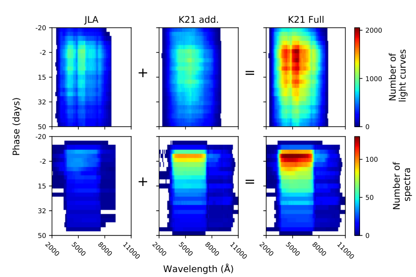
IV.1 The Pan-STARRS Medium Deep Survey
The Pan-STARRS medium deep survey covered 70 square degrees of sky over four years, discovering approximately 5200 SNe (Jones et al. 2017; Villar et al. 2020) and spectroscopically classifying 10% of these at a median redshift of 0.35 (Rest et al. 2014). The Pantheon analysis, which combined these data with JLA, includes 279 PS1-observed SNe Ia with an average of approximately 6 observations per 10 days in (Scolnic et al. 2018). We use these SNe Ia in our training data.
IV.2 The Foundation Supernova Survey
The Foundation Supernova Survey (Foley et al. 2018) followed SNe using the Pan-STARRS1 telescope, and measured well-calibrated SN light curves in filters with a five-day cadence near maximum light and an approximately 8-day cadence beginning at 10 days after maximum light. To achieve reduced selection effects compared to previous surveys that targeted bright, pre-selected low- galaxies, Foundation primarily followed SNe discovered by untargeted surveys such as the All-Sky Automated Survey for Supernovae (Shappee et al. 2014), the Asteroid Terrestrial-impact Last Alert System (Tonry et al. 2018), Gaia (Gaia Collaboration et al. 2016), and the Pan-STARRS Survey for Transients (Huber et al. 2015) .
The Foundation first data release in Foley et al. 2018 contains 225 SNe Ia, 180 of which are cosmologically useful. These data have been used to measure cosmological parameters in Jones et al. 2019 and the correlation of host galaxy properties with SN distances in Jones et al. 2018. The band coverage of Foundation is particularly critical to creating a SALT3 model that is trained to redder wavelengths than enabled by the JLA data alone. We include spectra for 114 Foundation SNe from the Dettman et al. 2021 data release.
IV.3 The Dark Energy Survey
The Dark Energy Survey (DES) three-year spectroscopically classified SN sample contains 207 SNe Ia at a median redshift of 0.36 (Abbott et al. 2019). These SNe were discovered by imaging eight 2.7 deg2 “shallow” fields (depth mag) and two 2.7 deg2 “deep” fields (depth mag) approximately once per week (Smith et al. 2020a). Transients were discovered using a difference-imaging pipeline (Kessler et al. 2015) and final photometry was performed with a “scene modeling” pipeline described in Brout et al. 2019b. See Abbott et al. 2019 and Brout et al. 2019a for additional details regarding the DES SN Ia data and analyses. These data have a maximum redshift of 0.85 and complement SNLS in probing rest-frame near-UV wavelengths with well-calibrated (sub-percent) photometric data (Burke et al. 2018).
| Survey | NSN | N | N | Filters | Ref. | |||
| (JLA) | (Total) | |||||||
| Calan-Tololo | 5 | 0 | 0 | 0.015 | 0.020 | 0.051 | Hamuy et al. 1996 | |
| CfA1 | 8 | 46 | 66 | 0.004 | 0.011 | 0.050 | Riess et al. 1999 | |
| CfA2 | 13 | 108 | 166 | 0.008 | 0.014 | 0.031 | Jha et al. 2006 | |
| CfA3c | 51 | 31 | 534 | 0.004 | 0.023 | 0.041 | Hicken et al. 2009b | |
| SDSSc | 202 | 0 | 12 | 0.037 | 0.166 | 0.250 | Holtzman et al. 2008 | |
| SNLS | 111 | 63 | 63 | 0.149 | 0.499 | 0.700 | Astier et al. 2006 | |
| Misc. low- | 25 | 152 | 216 | 0.001 | 0.009 | 0.077 | Jha et al. 2007 | |
| SALT2.JLA Total | 415 | 400 | 1057 | 0.001 | 0.172 | 0.700 | ||
| CfA4c | 30 | 0 | 0 | 0.009 | 0.029 | 0.070 | Hicken et al. 2012 | |
| CSP | 13 | 0 | 36 | 0.011 | 0.029 | 0.058 | Krisciunas et al. 2017 | |
| Foundation | 153 | 0 | 114 | 0.005 | 0.034 | 0.111 | Foley et al. 2018 | |
| PS1 MDSc | 266 | 0 | 0 | 0.026 | 0.297 | 0.630 | Scolnic et al. 2018 | |
| DES-spec | 206 | 0 | 0 | 0.078 | 0.362 | 0.850 | Abbott et al. 2019 | |
| New Data Total | 668 | 0 | 150 | 0.005 | 0.244 | 0.850 | ||
| SALT3 Total | 1083 | 400 | 1207 | 0.001 | 0.201 | 0.850 | ||
| Note. SNe Ia in the K21 compilation, after cuts: the original JLA training sample is reduced to 415 SNe (originally 420) and the new data adds 668 SNe, for a total of 1083 SNe. a Total number of spectra, rather than number of SNe with spectra, which is 83 for the JLA sample and an additional 297 from the new data included here. Spectra are from Filippenko et al. 1992; Wells et al. 1994; Patat et al. 1996; NAT 1997; Li et al. 2001; Salvo et al. 2001; Valentini et al. 2003; Anupama et al. 2005; Benetti et al. 2004; Kotak et al. 2005; Leonard et al. 2005; Garavini et al. 2007; Stanishev et al. 2007; Thomas et al. 2007; Foley et al. 2008; Pignata et al. 2008; Wang et al. 2009; Foley et al. 2010; Östman et al. 2011; Walker et al. 2011; Blondin et al. 2012; Silverman et al. 2012b; Folatelli et al. 2013; Balland et al. 2018 and from private communication with M. Betoule and C. Balland. b We note that these filter transmission curves were not provided for these samples. c 11 SNe in these samples have additional data from the CSP (Contreras et al. 2010; Krisciunas et al. 2017), while SDSS SNe 2006oa, 2006ob, 2006on, and 2006nz also have data from CfA3 (Hicken et al. 2009b). c See also Rest et al. 2014 and Jones et al. 2018. | ||||||||
IV.4 Sample Selection Cuts
To ensure that SNe are suitable for inclusion in a training sample, we first require that every SN in the compilation is a spectroscopically classified, Branch-normal SN Ia (Branch et al. 1993; we include 1991T-like SNe Ia following the original SALT2 training procedure; Guy et al. 2007). For the SN light curves, we make the following selection requirements (cuts):
- •
At least four epochs at phases between days, where is the rest-frame phase relative to time of B-band peak.
- •
At least one measurement after peak brightness (), to constrain the shape.
- •
At least one measurement in each of at least two filters at to constrain the color of the SN.
- •
At least one measurement prior to peak brightness () to ensure a well-measured time of maximum light. This is the only cut that was not included in the original SALT2 training44 4 5 of 420 SNe from the JLA sample are removed with this cut..
For the spectra, we include the original SALT2.JLA training spectra in addition to spectra taken from the kaepora database and spectra taken as part of the Foundation Supernova Survey. A number of these spectra were taken by the Foundation team, but most have been published on the Transient Name Server55 5 https://wis-tns.org/ as classification spectra.
To ensure minimal host galaxy contamination in the high- SN spectra used for model training, Guy et al. 2007 fit the spectra with a combined model including the predicted SN spectrum, the spectral recalibration parameters, and a galaxy model (elliptical, S0, Sa, Sb, and Sc templates). They removed spectra for which there was evidence for host galaxy contamination at the 68% confidence level.
For Foundation and the additional low- SN spectra included here, low- SNe are much brighter relative to their host galaxies than at the redshifts probed by SNLS and SDSS. We clip host galaxy lines, mask regions with uncorrected telluric features, and remove excessively noisy or poorly calibrated regions of each spectrum, but do not attempt to subtract a host galaxy continuum. We remove a handful of spectra with poor quality from visual inspection. After cuts there are 114 spectra from Foundation and 693 from Kaepora, a subset of which are shown in Section V. All but five Foundation SNe have redshifts measured from host galaxy features. The complete training data are available at https://saltshaker.readthedocs.io.
V The SALT3 Model: Extending the Wavelength Range and Training on Pantheon, Foundation, and DES Data
Having demonstrated the effectiveness of SALTshaker on the original JLA training data, we now train a SALT3 model using additional data, extending the free model parameters in SALTshaker in three ways. First, we extend the SED wavelength range to 11000 Å so that rest frame filters centered at wavelengths up to angstroms, such as the Foundation -band, can be fit with the model. Secondly, we extend the SED wavelength range over which the color law is fit with a polynomial (Eq. II) to 8000 Å , just below the central wavelength of the PS1 band. We use a fourth-order polynomial, rather than the third-order polynomial used for SALT2.JLA, to model the color law over the increased wavelength range with more training data. Third, the color scatter model is changed from a third to a fourth-order polynomial to allow additional flexibility over the increased wavelength range.
V.1 Validation on Extended Wavelength Range
Before presenting our model trained on all data in Section V.2, we check the performance on separate training and validation samples. We take the “K21valid” compilation as our cosmology sample using our “SALT3.K21train” model as described in Section III.1, and show the resulting Hubble residuals in Figure 8 and in row 3 of Table 5. We find that nuisance parameters are similar between SALT2.JLA and the SALT3.K21train model, with slightly higher by but with a consistent (the SALT3 RMS is negligibly smaller). is consistent with zero at the mmag level.
V.2 Training on Complete K21 Compilation
Finally, we train our best SALT3 model, which we call SALT3.K21, using all of the data described in previous sections as a training sample. The sample includes 1083 SNe, a factor of 2.5 more SNe than the JLA training sample, and 1207 spectra, a factor of three increase in the number of spectra. Synthetic light curves from SALT3.K21 and SALT2.JLA are compared in Figure 12 and the model uncertainties are compared in Figure 13. We see good consistency between SALT2.JLA and SALT3.K21, with modest differences in the -band and some additional differences in redder bands; at both wavelength ranges we have substantially increased the training sample (see Figure 10). Similarly, as shown in Figure 14, the color law is consistent with that of SALT2.JLA to within 1% across the entire wavelength range.
We compare Hubble residuals of the SALT3.K21 and SALT2.JLA models in Figure 8. Individual standardized distances are consistent to between the two models, and the effects on the Hubble diagram are found in row 4 of Table 5. is consistent with zero at . Finally, row 4 of Table 5 shows nuisance parameters and Hubble diagram metrics, demonstrating that SALTshaker produces a new SALT3 model with slightly lower total dispersion, consistent , and consistent distances. We note that the parameter is lower by 0.24 in the SALT3 model, likely due to a reconsidered separation of color and stretch.
V.2.1 Model Uncertainties and Hubble Scatter of SALT3.K21
The uncertainties in Figure 13 show that both the color scatter and light-curve uncertainties in redder bands are much lower in SALT3.K21 than SALT2.JLA. The SALT2 color scatter was effectively unconstrained by the JLA data past mean passband wavelengths Å, and we find that while the color scatter is significant at these wavelengths, it is much smaller than implied by the SALT2.JLA model. Our additional data constrains this region up to Å, and redder data will be required to see how this effect carries into the NIR. We also note lower color scatter by in the blue, which we attribute to improved relative calibration of the training sample.
Fitting the light curves using the SALT3.K21 model, we compare the uncertainties in distances and light-curve parameters to those found using SALT2.JLA. In Figure 11 we compare performance across the redshift range. Our model shows reduced Hubble scatter and distance uncertainties over the SALT2.JLA model at nearly every redshift, with the least improvement at moderate redshifts , where signal to noise is high and the SALT2.JLA model is already performing well. Light-curve parameters from SALT3.K21train have smaller uncertainties across the redshift range, with the exception of uncertainties. Our largest improvements, particularly in color uncertainty, are found at low redshift, where the improved red wavelength coverage of our model allows the use of additional light curve bands in fitting these SNe, providing stronger constraints.
There is a slight improvement in RMS Hubble residuals, largely attributable to decreased color uncertainties in the low redshift sample. Breaking this down further, Figure 15 shows the Hubble scatter binned by the number of additional filters used in the SALT3.K21 light-curve fit as compared to the SALT2.JLA light-curve fit in Figure 15. Where two additional filters are available, RMS improves by . We conclude improvement in the SALT3 model is most noticeable when it allows us to fit SNe with existing light curves in filters out of the SALT2.JLA wavelength range. At high redshift, SALT3’s improved constraints on the NUV model reduce Hubble scatter by mag, although there is typically not sufficiently red data to take full advantage of the extended wavelength range at these redshifts. Similarly, when breaking down results by survey, as we show in Figure 15, the greatest improvement is in the low- CFA3 and Foundation samples where we can make use of and band observations (respectively) previously unused in SALT2.JLA-based analyses at low redshift. We are able to reduce the RMS of the Foundation sample from mag to 0.125 mag, an improvement of 15%.
V.2.2 Comparison of SALT3.K21 and SALT2.JLA Light-curve Parameters
The SALTshaker training procedure results in different distributions of light-curve parameters compared to SALT2.JLA. Some differences are due to changes in how the SALT3 model is defined, while others are from the demographics of the training sample. For example, a / degeneracy is broken by setting a constraint on the standard deviation , both in our procedure and in the original training procedure; therefore including additional data with higher stretch increases the scale of the component.
In Figure 16 we compare the distributions of the and parameters from both models. We note a slight rotation, shift, and scale change of the color/stretch distribution relative to SALT2.JLA. These linear transformations cancel in the Tripp standardization of distance, absorbed into the nuisance parameters . The offset in color in particular is from including bluer high redshift SNe from PS1 and DES in the training sample. The rotation is due to the distinct procedures for separating stretch and color between the SALT2 training code and SALTshaker. SALT3.K21 and values can be approximated from the SALT2.JLA values by the transformations
| (18) | ||||
| (19) |
To test the similarity of the shape of the distributions, we use the two dimensional Kolmogorov-Smirnov -like test statistic of Press & Teukolsky 1988. We modify the procedure by linearly transforming both sets of light-curve parameters to have the same mean, standard deviation, and - correlation before calculating the statistic. We find the test statistic for the SALT2.JLA and SALT3.K21 and parameters, then bootstrap resample the data and calculate the test statistic with the resampled data. We derive a p-value, and conclude that we cannot distinguish the shape of the underlying distributions.
| Sample | Nuisance Parameters | Hubble Flow Dist. | ||||||
| Model | Validation Sample | RMS | ||||||
| SALT2.JLA | 420 | large sim. JLAb | 0.173 | |||||
| 1 | SALT3.simJLA | 420 | large sim. JLAb | 0.182 | ||||
| SALT2.JLA | 420 | JLA | 0.153 | |||||
| 2 | SALT3.JLA | 420 | JLA | 0.155 | ||||
| SALT2.JLA | 420 | K21 Valid | 0.148 | |||||
| 3 | SALT3.K21train | 541 | K21 Valid | 0.152 | ||||
| SALT2.JLA | 420 | K21 Full | 0.146 | |||||
| 4 | SALT3.K21 | 1083 | K21 Full | 0.143 | ||||
| Cosmological results from light-curve fits using SALT3 models created with different training sets, compared to results when using the SALT2.JLA model. Training sets include a simulated JLA training sample (simJLA, Row 1), the real JLA training sample (JLA, Row 2), an expanded training sample using the full JLA training sample but including only half the additional data we use, with the remainder used for validation (K21train, Row 3), and the full K21 compilation (highlighted in Row 4), which is the training sample used to create the SALT3 model published in this work. Our best model using the complete K21 compilation results in nuisance parameters and distances statistically consistent but slightly lower Hubble scatter as compared to SALT2. a Relative to the equivalent SALT2 fitting results, the distance between average Hubble residual at and the average Hubble residual at . b Large, combined simulations of CfA3, SDSS, and SNLS with a total of 3000 SNe to measure distance biases more precisely than is possible from a sample with the size of the JLA training sample | ||||||||
VI Conclusions
We have presented SALTshaker, a new Python-based training code to train a phenomenologically motivated light-curve model using the SALT framework, in addition to a retrained SALT model we call SALT3. SALTshaker is publicly available at https://github.com/djones1040/SALTShaker with documentation at https://saltshaker.readthedocs.io/en/latest/. The SALTshaker documentation includes links to the training data and the SALT3.K21 model, and the SALT3.K21 model is compatible with and included in the latest versions of SNANA and sncosmo.
The SALT3.K21 model itself includes updated calibration with Supercal, a training sample with 1083 SNe 2.5 times larger than previous training samples and extends to the rest-frame bands. Due to its larger wavelength range, we find that SALT3.K21 distances for both legacy low- data and Foundation data are approximately 15% more precise, equivalent to increasing the low- sample size by 30%. The SALT3.K21 model is based on updated calibration with Supercal (Scolnic et al. 2015) and revised MW E(B-V) estimates from Schlafly & Finkbeiner 2011. As part of an upcoming cosmology analysis we have employed SALT3.K21 within the PIPPIN (Hinton & Brout 2020) framework, generating simulations and performing bias corrections following the methodologies of Kessler et al. 2019 and Kessler & Scolnic 2017. Although this work is preliminary, we find that cosmological parameters found using a larger light-curve dataset of SNe Ia (to be released in Brout+ in prep) are consistent between SALT3.K21 and SALT2.JLA. Looking to future missions, we find that for the forecast SN Ia survey of the Roman Space Telescope, assuming the ALL strategy (Hounsell et al. 2018), the extended wavelength range in SALT3.K21 makes use of more observations compared to SALT2.JLA; this increase is about a factor of 2 for redshifts , and falls to about a 10% increase at .
Several light-curve models have been developed for cosmological supernovae, including MLCS (Riess et al. 1996), MLCS2k2 (Jha et al. 2007), SiFTO (Conley et al. 2008), SNooPy (Burns et al. 2011), SNEMO (Saunders et al. 2018), SUGAR (Léget et al. 2019), and BayesSN (Mandel et al. 2011; Mandel et al. 2020). In the context of other modern light-curve models, SALT3 offers an approach to model design and training process that prioritizes the use of heterogeneous spectral and photometric data to provide extensive phase and wavelength coverage and native k-corrections through cosmology-independent training. The model framework is minimally changed from SALT2, so SNANA simulations, bias corrections, and other analysis products are expected to require little revision.
Over the coming years, we expect SALTshaker will continue to be developed and improved as additional SN data becomes available and additional SN standardization parameters (e.g., host mass) are discovered and explored. Further development work could focus on the error model, which is currently based on central filter wavelengths rather than integrated quantities. This is a potential source of systematic uncertainty because observer-frame filter functions are contracted in the rest frame. Additionally, SALTshaker enables a more rigorous evaluation of systematic uncertainties such as those arising from limited training data, photometric calibration uncertainties, or treatment of SN spectra. These can be evaluated in a straightforward and rigorous way by re-training the SALT3 model surfaces on simulated data. Although we have demonstrated that SALTshaker can faithfully recover a truth model at the 1% level, future work will also be able to fully validate the model training process using an entire analysis chain that includes training, bias corrections, and cosmology fitting (Dai et al in prep). Similarly, while the SALT3 model surfaces presented in this work have been trained on data recalibrated to the level of via the Supercal procedure (Scolnic et al. 2015; Scolnic et al. 2018), we have left quantifying the reduced calibration uncertainties as a topic for further work.
The BYOSED code (Pierel et al. 2020) implements a range of simulated effects to a base SED template, such as perturbations to line velocity, multiple sources of reddening with distinct effects, and correlations of host galaxy properties with the SN Ia SED. Future work could perform the SALTshaker method on a BYOSED-produced training sample with such underlying effects. By propagating any biases introduced by the training code into cosmology, we may quantify the potential impact of currently unmodeled supernova phenomenology on cosmology.
Samples of SN Ia light curves will increase by orders of magnitude with the Vera Rubin Telescope’s LSST (Ivezić et al. 2019) and the Roman Space Telescope (Hounsell et al. 2018). For error budgets to continue improvement, light-curve models should not be tied to outdated calibration standards, and it is essential that the model training process be regarded as a key component of an integrated cosmology analysis, as has been done in Betoule et al. 2014 and Mosher et al. 2014.
References
- NAT (1997) 1997, NATO Advanced Study Institute (ASI) Series C, Vol. 486, Thermonuclear supernovae
- Abbott et al. (2019) Abbott, T. M. C., Allam, S., Andersen, P., et al. 2019, ApJ, 872, L30
- Anupama et al. (2005) Anupama, G. C., Sahu, D. K., & Jose, J. 2005, A&A, 429, 667
- Astier et al. (2006) Astier, P., Guy, J., Regnault, N., et al. 2006, A&A, 447, 31
- Astropy Collaboration et al. (2013) Astropy Collaboration, Robitaille, T. P., Tollerud, E. J., et al. 2013, A&A, 558, A33
- Astropy Collaboration et al. (2018) Astropy Collaboration, Price-Whelan, A. M., Sipőcz, B. M., et al. 2018, AJ, 156, 123
- Avelino et al. (2019) Avelino, A., Friedman, A. S., Mandel, K. S., et al. 2019, ApJ, 887, 106
- Balland et al. (2018) Balland, C., Cellier-Holzem, F., Lidman, C., et al. 2018, A&A, 614, A134
- Barbary (2016) Barbary, K. 2016, extinction v0.3.0
- Barbary et al. (2015) Barbary, K., rbiswas4, Rodney, S., et al. 2015, Sncosmo: V1.0.0
- Barbary et al. (2016) Barbary, K., Barclay, T., Biswas, R., et al. 2016, SNCosmo: Python library for supernova cosmology
- Benetti et al. (2004) Benetti, S., Meikle, P., Stehle, M., et al. 2004, MNRAS, 348, 261
- Betoule et al. (2014) Betoule, M., Kessler, R., Guy, J., et al. 2014, Astronomy & Astrophysics, 568, A22
- Blondin et al. (2012) Blondin, S., Matheson, T., Kirshner, R. P., et al. 2012, AJ, 143, 126
- Branch et al. (1993) Branch, D., Fisher, A., & Nugent, P. 1993, AJ, 106, 2383
- Brout et al. (2020) Brout, D., Hinton, S., & Scolnic, D. 2020, arXiv e-prints, arXiv:2012.05900
- Brout & Scolnic (2020) Brout, D., & Scolnic, D. 2020
- Brout et al. (2019a) Brout, D., Scolnic, D., Kessler, R., et al. 2019a, ApJ, 874, 150
- Brout et al. (2019b) Brout, D., Sako, M., Scolnic, D., et al. 2019b, ApJ, 874, 106
- Burke et al. (2018) Burke, D. L., Rykoff, E. S., Allam, S., et al. 2018, AJ, 155, 41
- Burns et al. (2011) Burns, C. R., Stritzinger, M., Phillips, M. M., et al. 2011, The Astronomical Journal, 141, 19
- Cardelli et al. (1989) Cardelli, J. A., Clayton, G. C., & Mathis, J. S. 1989, ApJ, 345, 245
- Chotard et al. (2011) Chotard, N., Gangler, E., Aldering, G., et al. 2011, Astronomy & Astrophysics, 529, L4
- Conley et al. (2008) Conley, A., Sullivan, M., Hsiao, E. Y., et al. 2008, The Astrophysical Journal, 681, 482
- Conley et al. (2011) Conley, A., Guy, J., Sullivan, M., et al. 2011, The Astrophysical Journal Supplement Series, 192, 1
- Contreras et al. (2010) Contreras, C., Hamuy, M., Phillips, M. M., et al. 2010, The Astronomical Journal, 139, 519
- da Costa-Luis et al. (2021) da Costa-Luis, C., Larroque, S. K., Altendorf, K., et al. 2021, tqdm: A fast, Extensible Progress Bar for Python and CLI
- Dembinski et al. (2020) Dembinski, H., Ongmongkolkul, P., Deil, C., et al. 2020, scikit-hep/iminuit: v1.4.9
- Dettman et al. (2021) Dettman, K. G., Jha, S. W., Dai, M., et al. 2021, arXiv e-prints, arXiv:2102.06524
- Dhawan et al. (2018) Dhawan, S., Jha, S. W., & Leibundgut, B. 2018, Astronomy & Astrophysics, 609, A72
- Filippenko et al. (1992) Filippenko, A. V., Richmond, M. W., Matheson, T., et al. 1992, ApJ, 384, L15
- Fitzpatrick (1999) Fitzpatrick, E. L. 1999, PASP, 111, 63
- Folatelli et al. (2013) Folatelli, G., Morrell, N., Phillips, M. M., et al. 2013, ApJ, 773, 53
- Foley et al. (2008) Foley, R. J., Filippenko, A. V., & Jha, S. W. 2008, ApJ, 686, 117
- Foley & Kasen (2011) Foley, R. J., & Kasen, D. 2011, ApJ, 729, 55
- Foley et al. (2010) Foley, R. J., Narayan, G., Challis, P. J., et al. 2010, ApJ, 708, 1748
- Foley et al. (2018) Foley, R. J., Scolnic, D., Rest, A., et al. 2018, MNRAS, 475, 193
- Freedman et al. (2019) Freedman, W. L., Madore, B. F., Hatt, D., et al. 2019, The Astrophysical Journal, 882, 34
- Gaia Collaboration et al. (2016) Gaia Collaboration, Prusti, T., de Bruijne, J. H. J., et al. 2016, A&A, 595, A1
- Garavini et al. (2007) Garavini, G., Nobili, S., Taubenberger, S., et al. 2007, A&A, 471, 527
- Ginsburg et al. (2019) Ginsburg, A., Sipőcz, B. M., Brasseur, C. E., et al. 2019, AJ, 157, 98
- Guy et al. (2007) Guy, J., Astier, P., Baumont, S., et al. 2007, Astronomy & Astrophysics, 466, 11
- Guy et al. (2010) Guy, J., Sullivan, M., Conley, A., et al. 2010, Astronomy & Astrophysics, 523, A7
- Hamuy et al. (1996) Hamuy, M., Phillips, M. M., Suntzeff, N. B., et al. 1996, AJ, 112, 2408
- Harris et al. (2020) Harris, C. R., Millman, K. J., van der Walt, S. J., et al. 2020, Nature, 585, 357
- Hicken et al. (2009a) Hicken, M., Wood-Vasey, W. M., Blondin, S., et al. 2009a, The Astrophysical Journal, 700, 1097
- Hicken et al. (2009b) Hicken, M., Challis, P., Jha, S., et al. 2009b, The Astrophysical Journal, 700, 331
- Hicken et al. (2012) Hicken, M., Challis, P., Kirshner, R. P., et al. 2012, The Astrophysical Journal Supplement Series, 200, 12
- Hinton & Brout (2020) Hinton, S., & Brout, D. 2020, Journal of Open Source Software, 5, 2122
- Holtzman et al. (2008) Holtzman, J. A., Marriner, J., Kessler, R., et al. 2008, AJ, 136, 2306
- Hounsell et al. (2018) Hounsell, R., Scolnic, D., Foley, R. J., et al. 2018, ApJ, 867, 23
- Huber et al. (2015) Huber, M., Chambers, K. C., Flewelling, H., et al. 2015, The Astronomer’s Telegram, 7153, 1
- Hunter (2007) Hunter, J. D. 2007, Computing in Science & Engineering, 9, 90
- Ivezić et al. (2019) Ivezić, Ž., Kahn, S. M., Tyson, J. A., et al. 2019, ApJ, 873, 111
- James & Roos (1975) James, F., & Roos, M. 1975, Computer Physics Communications, 10, 343
- Jha et al. (2007) Jha, S., Riess, A. G., & Kirshner, R. P. 2007, The Astrophysical Journal, 659, 122
- Jha et al. (2006) Jha, S., Kirshner, R. P., Challis, P., et al. 2006, The Astronomical Journal, 131, 527
- Jones et al. (2017) Jones, D. O., Scolnic, D. M., Riess, A. G., et al. 2017, ApJ, 843, 6
- Jones et al. (2018) Jones, D. O., Riess, A. G., Scolnic, D. M., et al. 2018, The Astrophysical Journal, 867, 108
- Jones et al. (2019) Jones, D. O., Scolnic, D. M., Foley, R. J., et al. 2019, The Astrophysical Journal, 881, 19
- Kelly et al. (2010) Kelly, P. L., Hicken, M., Burke, D. L., Mand el, K. S., & Kirshner, R. P. 2010, ApJ, 715, 743
- Kessler & Scolnic (2017) Kessler, R., & Scolnic, D. 2017, ApJ, 836, 56
- Kessler & Scolnic (2017) Kessler, R., & Scolnic, D. 2017, The Astrophysical Journal, 836, 56
- Kessler et al. (2009a) Kessler, R., Becker, A. C., Cinabro, D., et al. 2009a, The Astrophysical Journal Supplement Series, 185, 32
- Kessler et al. (2009b) Kessler, R., Bernstein, J. P., Cinabro, D., et al. 2009b, Publications of the Astronomical Society of the Pacific, 121, 1028
- Kessler et al. (2009c) —. 2009c, Publications of the Astronomical Society of the Pacific, 121, 1028
- Kessler et al. (2015) Kessler, R., Marriner, J., Childress, M., et al. 2015, AJ, 150, 172
- Kessler et al. (2019) Kessler, R., Brout, D., D’Andrea, C. B., et al. 2019, MNRAS, 485, 1171
- Kessler et al. (2019) Kessler, R., et al. 2019, Mon. Not. Roy. Astron. Soc., 485, 1171
- Kotak et al. (2005) Kotak, R., Meikle, W. P. S., Pignata, G., et al. 2005, A&A, 436, 1021
- Krisciunas et al. (2004) Krisciunas, K., Suntzeff, N. B., Phillips, M. M., et al. 2004, AJ, 128, 3034
- Krisciunas et al. (2007) Krisciunas, K., Garnavich, P. M., Stanishev, V., et al. 2007, AJ, 133, 58
- Krisciunas et al. (2017) Krisciunas, K., Contreras, C., Burns, C. R., et al. 2017, The Astronomical Journal, 154, 211
- Léget et al. (2019) Léget, P. F., Gangler, E., Mondon, F., et al. 2019
- Leonard et al. (2005) Leonard, D. C., Li, W., Filippenko, A. V., Foley, R. J., & Chornock, R. 2005, ApJ, 632, 450
- Li et al. (2001) Li, W., Filippenko, A. V., Treffers, R. R., et al. 2001, ApJ, 546, 734
- Mandel et al. (2011) Mandel, K. S., Narayan, G., & Kirshner, R. P. 2011, The Astrophysical Journal, 731, 120
- Mandel et al. (2020) Mandel, K. S., Thorp, S., Narayan, G., Friedman, A. S., & Avelino, A. 2020, arXiv e-prints, arXiv:2008.07538
- Marriner et al. (2011) Marriner, J., Bernstein, J. P., Kessler, R., et al. 2011, The Astrophysical Journal, 740, 72
- Marwil (1979) Marwil, E. 1979, SIAM Journal on Numerical Analysis, 16, 588
- Mosher et al. (2014) Mosher, J., Guy, J., Kessler, R., et al. 2014, The Astrophysical Journal, 793, 16
- Östman et al. (2011) Östman, L., Nordin, J., Goobar, A., et al. 2011, A&A, 526, A28
- Patat et al. (1996) Patat, F., Benetti, S., Cappellaro, E., et al. 1996, MNRAS, 278, 111
- Perlmutter et al. (1999) Perlmutter, S., Aldering, G., Goldhaber, G., et al. 1999, The Astrophysical Journal, 517, 565
- Pierel et al. (2018) Pierel, J. D. R., Rodney, S., Avelino, A., et al. 2018, PASP, 130, 114504
- Pierel et al. (2020) Pierel, J. D. R., Jones, D. O., Dai, M., et al. 2020, arXiv e-prints, arXiv:2012.07811
- Pignata et al. (2008) Pignata, G., Benetti, S., Mazzali, P. A., et al. 2008, MNRAS, 388, 971
- Press & Teukolsky (1988) Press, W. H., & Teukolsky, S. A. 1988, Computers in Physics, 2, 74
- Rest et al. (2014) Rest, A., Scolnic, D., Foley, R. J., et al. 2014, ApJ, 795, 44
- Riess et al. (2021) Riess, A. G., Casertano, S., Yuan, W., et al. 2021, ApJ, 908, L6
- Riess et al. (1996) Riess, A. G., Press, W. H., & Kirshner, R. P. 1996, ApJ, 473, 88
- Riess et al. (1998) Riess, A. G., Filippenko, A. V., Challis, P., et al. 1998, The Astronomical Journal, 116, 1009
- Riess et al. (1999) Riess, A. G., Kirshner, R. P., Schmidt, B. P., et al. 1999, The Astronomical Journal, 117, 707
- Riess et al. (2016) Riess, A. G., Macri, L. M., Hoffmann, S. L., et al. 2016, The Astrophysical Journal, 826, 56
- Riess et al. (2018) Riess, A. G., Rodney, S. A., Scolnic, D. M., et al. 2018, The Astrophysical Journal, 853, 126
- Rigault et al. (2013) Rigault, M., Copin, Y., Aldering, G., et al. 2013, A&A, 560, A66
- Rigault et al. (2018) Rigault, M., Brinnel, V., Aldering, G., et al. 2018
- Rose et al. (2020) Rose, B. M., Dixon, S., Rubin, D., et al. 2020, ApJ, 890, 60
- Rubin (2020) Rubin, D. 2020, ApJ, 897, 40
- Sako et al. (2018) Sako, M., Bassett, B., Becker, A. C., et al. 2018, Publications of the Astronomical Society of the Pacific, 130, 064002
- Salvo et al. (2001) Salvo, M. E., Cappellaro, E., Mazzali, P. A., et al. 2001, MNRAS, 321, 254
- Saunders et al. (2018) Saunders, C., Aldering, G., Antilogus, P., et al. 2018, The Astrophysical Journal, 869, 167
- Schlafly & Finkbeiner (2011) Schlafly, E. F., & Finkbeiner, D. P. 2011, ApJ, 737, 103
- Schlegel et al. (1998) Schlegel, D. J., Finkbeiner, D. P., & Davis, M. 1998, ApJ, 500, 525
- Schubert (1970) Schubert, L. K. 1970, Mathematics of Computation, 24, 27
- Scolnic & Kessler (2016) Scolnic, D., & Kessler, R. 2016, ApJ, 822, L35
- Scolnic et al. (2015) Scolnic, D., Casertano, S., Riess, A., et al. 2015, The Astrophysical Journal, 815, 117
- Scolnic et al. (2018) Scolnic, D. M., Jones, D. O., Rest, A., et al. 2018, The Astrophysical Journal, 859, 101
- Shappee et al. (2014) Shappee, B. J., Prieto, J. L., Grupe, D., et al. 2014, ApJ, 788, 48
- Siebert et al. (2020) Siebert, M. R., Foley, R. J., Jones, D. O., & Davis, K. W. 2020, MNRAS, 493, 5713
- Siebert et al. (2019) Siebert, M. R., Foley, R. J., Jones, D. O., et al. 2019, MNRAS, 486, 5785
- Silverman et al. (2012a) Silverman, J. M., Foley, R. J., Filippenko, A. V., et al. 2012a, MNRAS, 425, 1789
- Silverman et al. (2012b) —. 2012b, MNRAS, 425, 1789
- Smith et al. (2020a) Smith, M., D’Andrea, C. B., Sullivan, M., et al. 2020a, AJ, 160, 267
- Smith et al. (2020b) Smith, M., Sullivan, M., Wiseman, P., et al. 2020b, MNRAS, 494, 4426
- Stahl et al. (2020) Stahl, B. E., Zheng, W., de Jaeger, T., et al. 2020, MNRAS, 492, 4325
- Stanishev et al. (2007) Stanishev, V., Goobar, A., Benetti, S., et al. 2007, A&A, 469, 645
- Sullivan et al. (2010) Sullivan, M., Conley, A., Howell, D. A., et al. 2010, Monthly Notices of the Royal Astronomical Society, 406, no
- Taylor et al. (2021) Taylor, G., Lidman, C., Tucker, B. E., et al. 2021, arXiv e-prints, arXiv:2104.00172
- The LSST Dark Energy Science Collaboration et al. (2018) The LSST Dark Energy Science Collaboration, Mandelbaum, R., Eifler, T., et al. 2018, arXiv e-prints, arXiv:1809.01669
- Thomas et al. (2007) Thomas, R. C., Aldering, G., Antilogus, P., et al. 2007, ApJ, 654, L53
- Tonry et al. (2018) Tonry, J. L., Denneau, L., Heinze, A. N., et al. 2018, PASP, 130, 064505
- Tripp (1998) Tripp, R. 1998, A&A, 331, 815
- Valentini et al. (2003) Valentini, G., Di Carlo, E., Massi, F., et al. 2003, ApJ, 595, 779
- Verde et al. (2019) Verde, L., Treu, T., & Riess, A. G. 2019
- Villar et al. (2020) Villar, V. A., Hosseinzadeh, G., Berger, E., et al. 2020, arXiv e-prints, arXiv:2008.04921
- Virtanen et al. (2020) Virtanen, P., Gommers, R., Oliphant, T. E., et al. 2020, Nature Methods, 17, 261
- Walker et al. (2011) Walker, E. S., Hook, I. M., Sullivan, M., et al. 2011, MNRAS, 410, 1262
- Wang et al. (2009) Wang, X., Li, W., Filippenko, A. V., et al. 2009, ApJ, 697, 380
- Wells et al. (1994) Wells, L. A., Phillips, M. M., Suntzeff, B., et al. 1994, AJ, 108, 2233
- Wood-Vasey et al. (2008) Wood-Vasey, W. M., Friedman, A. S., Bloom, J. S., et al. 2008, ApJ, 689, 377