PHANGS–ALMA: Arcsecond CO(2–1) Imaging of Nearby Star-Forming Galaxies aplpy, ALMA Calibration Pipeline (L. Davis et al. in preparation), CASA (McMullin et al. 2007), numpy (Oliphant 2006), scipy (Virtanen et al. 2020), astropy (Astropy Collaboration et al. 2013; Astropy Collaboration et al. 2018), IDL Astronomy User’s Library (Landsman 1993), cprops (Rosolowsky & Leroy 2006), GILDAS Pety 2005, PHANGS–ALMA Pipeline (Leroy et al. 2021), PHANGS–ALMA Total Power Pipeline (Herrera et al. 2020), R (R Core Team 2015), spectral-cube (Ginsburg et al. 2019), radio-beam (https://github.com/radio-astro-tools/radio-beam)
Abstract
We present PHANGS–ALMA, the first survey to map CO line emission at pc spatial resolution from a representative sample of nearby ( Mpc) galaxies that lie on or near the “main sequence” of star-forming galaxies. CO line emission traces the bulk distribution of molecular gas, which is the cold, star-forming phase of the interstellar medium. At the resolution achieved by PHANGS–ALMA, each beam reaches the size of a typical individual giant molecular cloud (GMC), so that these data can be used to measure the demographics, life-cycle, and physical state of molecular clouds across the population of galaxies where the majority of stars form at . This paper describes the scientific motivation and background for the survey, sample selection, global properties of the targets, ALMA observations, and characteristics of the delivered ALMA data and derived data products. As the ALMA sample serves as the parent sample for parallel surveys with VLT/MUSE, HST, AstroSat, VLA, and other facilities, we include a detailed discussion of the sample selection. We detail the estimation of galaxy mass, size, star formation rate, CO luminosity, and other properties, compare estimates using different systems and provide best-estimate integrated measurements for each target. We also report the design and execution of the ALMA observations, which combine a Cycle 5 Large Program, a series of smaller programs, and archival observations. Finally, we present the first resolution atlas of CO emission from nearby galaxies and describe the properties and contents of the first PHANGS–ALMA public data release.
I Introduction
This paper presents PHANGS--ALMA, an Atacama Large Millimeter/submillimeter Array (ALMA) survey aimed at studying the physics of molecular gas across the nearby galaxy population. PHANGS--ALMA is a key component of the multiwavelength observational campaign conducted by the Physics at High Angular resolution in Nearby Galaxies (PHANGS) project22 2 http://phangs.org/. Combining a Cycle 5 ALMA Large Program, a suite of smaller programs, and data from the ALMA archive, PHANGS–ALMA mapped the CO emission, hereafter CO(), from a cleanly-selected sample of of the nearest, ALMA-accessible, massive, star-forming galaxies. The resulting CO() data have high spatial and spectral resolution, good surface brightness sensitivity, full flux recovery, and good coverage of the area of active star formation in each target.
These characteristics make PHANGS–ALMA the first “cloud scale,” pc, survey of molecular gas across a local galaxy sample that is representative of where stars form in the universe. Though the data are suitable for many scientific applications, the survey was designed with the broad goals of quantifying the physics of star formation and feedback at the scale of individual giant molecular clouds (GMCs) and connecting these measurements to galaxy-scale properties and processes.
With these goals in mind, the PHANGS team has followed up PHANGS–ALMA with a suite of multi-wavelength programs that span the spectrum from far-UV to radio, aiming to sample all stages of the star formation and feedback cycle. “PHANGS–MUSE” is obtaining optical integral field spectroscopy using the VLT/MUSE instrument to measure the properties of ionized gas and stellar populations at resolution matched to ALMA (PI: E. Schinnerer; E. Emsellem et al. in preparation). “PHANGS–HST” is using HST/WFC3 five-filter broad-band imaging to find and characterize stellar clusters and associations (Lee et al. 2021, PI: J. Lee;). Other programs include new, high resolution far-UV mapping by AstroSAT (PI: E. Rosolowsky), new ground-based narrow-band H imaging using the MPG 2.2m/WFI and Du Pont/DirectCCD instruments (PIs: G. Blanc, I-T. Ho; A. Razza et al. in preparation), and new Hi imaging using the VLA and MeerKAT (PI: D. Utomo; D. Utomo et al. in preparation).
This paper begins with an overview of the background, design, and goals of PHANGS–ALMA (§II). Because PHANGS–ALMA served as the parent sample for many of the multi-wavelength efforts descibed above, we discuss the sample selection in some detail in §III. We also present our best estimates for the integrated properties of our target galaxies in §IV. In §V, we describe the ALMA observations. A full description of our data processing pipeline is presented in a companion paper (Leroy et al. 2021), and we summarize our approach in §VI. In §VII, we describe the properties of the science-ready data products. Then we present an atlas of the PHANGS–ALMA data in §VIII. We give a brief summary in §IX.
II Scientific Motivation
II.1 Background
II.1.1 Previous Surveys of Molecular Gas in Galaxies
Much of our knowledge about the behavior of the molecular interstellar medium (ISM) in galaxies has been established by CO surveys that either integrate over whole galaxies (e.g., the FCRAO survey, Young et al. 1995; AMIGA, Lisenfeld et al. 2011; COLD GASS, Saintonge et al. 2011; ALLSMOG, Bothwell et al. 2014; xCOLD GASS Saintonge et al. 2017, and JINGLE, Saintonge et al. 2018) or resolve the large-scale structure of galaxy disks but do not distinguish individual molecular clouds (e.g., BIMA SONG, Helfer et al. 2003; the Nobeyama CO Atlas, Kuno et al. 2007; HERACLES, Leroy et al. 2009, the JCMT NGLS, Wilson et al. 2012; CARMA STING, Rahman et al. 2012; ATLAS–3D CO, Alatalo et al. 2013; Davis et al. 2014; CARMA EDGE Bolatto et al. 2017; NRO COMING, Sorai et al. 2019; and ALMAQUEST, Lin et al. 2019).
These surveys have demonstrated a close link between molecular gas and star formation, showing that the location and rate of recent star formation in a galaxy tracks the distribution of molecular gas (Wong & Blitz 2002; Kennicutt et al. 2007; Bigiel et al. 2008; Leroy et al. 2008; Schruba et al. 2011, e.g.,). Yet despite this good overall correspondence, observations reveal important variations in the amount of star formation per unit molecular gas both among different types of galaxies (e.g., Saintonge et al. 2011; Leroy et al. 2013b; Davis et al. 2014; Huang & Kauffmann 2015, and see Figure 1) and within different regions of the same galaxy (Longmore et al. 2013; Leroy et al. 2013b; Meidt et al. 2013; Momose et al. 2013; Leroy et al. 2017; Utomo et al. 2017; Brownson et al. 2020, e.g.,). The normalized CO emission of galaxies also varies, with CO emission appearing fainter relative to starlight or tracers of recent star formation in low mass and early-type galaxies (Young & Scoville 1991; Young et al. 1996; Schruba et al. 2012; Hunt et al. 2015; Saintonge et al. 2016; Saintonge et al. 2017, e.g.,). This change in brightness arises from both changes in molecular gas content and changes in CO emissivity per unit of molecular gas mass, but the relative magnitude of these effects is uncertain (Bolatto et al. 2013b, for a review see).
Figure 1 illustrates some of these global trends using data from PHANGS–ALMA (red, see §IV for details), xCOLD GASS (Saintonge et al. 2017) as the largest homogeneous unresolved survey, and a compilation of local CO mapping surveys (COMING, the Nobeyama CO Atlas, HERACLES, and a HERA follow up survey; Sorai et al. 2019; Kuno et al. 2007; Leroy et al. 2009, and A. Schruba et al. in preparation). The top panels show how the ratios of molecular gas mass to star formation rate and molecular gas mass to stellar mass change across the local galaxy population. The lower panels show the relationship between the average surface densities of molecular gas, stars, and star formation. Together, the four panels of Figure 1 demonstrate the good overall correspondence between star formation, stellar mass, and molecular gas in galaxies, but also illustrate important variations in the molecular content of galaxies normalized by size, star formation rate, or stellar mass. The abundance, structure, and ability of molecular gas to form stars varies across the galaxy population.
II.1.2 Key Physics at or Near Cloud Scales
Unfortunately, low resolution observations offer limited insight into the physical state of molecular gas. In the Milky Way and its Local Group neighbors, most of the molecular gas resides in GMCs with masses M⊙. These clouds have sizes of tens of parsecs and appear dominated by supersonic turbulence (Solomon et al. 1987; Blitz et al. 2007; Fukui & Kawamura 2010; Roman-Duval et al. 2010; Gratier et al. 2012; Heyer & Dame 2015; Rice et al. 2016; Miville-Deschênes et al. 2017; Schruba et al. 2019, e.g.,).
GMCs do not fill the galaxy disk. In low resolution extragalactic observations like those mentioned in the previous section, the CO emission from GMCs is diluted with nearby non-CO emitting regions. That is, the intrinsic distribution of CO emission in galaxies is strongly clumped on scales much smaller than the kiloparsec resolution of the previous generation of large CO mapping surveys (Leroy et al. 2013a, e.g.,). Figure 2 illustrates this phenomenon by showing CO emission from two PHANGS–ALMA targets at two resolutions: kpc and pc resolution. The sharp, clumpy structure that is striking in maps at high resolution (right panels), blurs into faint, low-contrast structures when observed at kiloparsec resolution (left panels).
Current models of star formation predict a link between star formation, feedback, and gas properties on the scale of individual GMCs, which can be inferred using high resolution observations. For example, the mean density and density distribution within a cloud may set the characteristic timescale for star formation (Padoan & Nordlund 2002; Hennebelle & Chabrier 2011; Krumholz & McKee 2005; Federrath & Klessen 2012; Krumholz & Dekel 2012, e.g.,). The strength of self-gravity in the cloud relative to turbulence and magnetic fields may affect the efficiency with which gas is converted into stars (Padoan et al. 2012; Padoan et al. 2017; Burkhart 2018; Kim et al. 2020b, e.g.,). The density, turbulence, and self-gravity may also determine how the new-born stars cluster (Kruijssen 2012; Hopkins 2013; Grudić et al. 2020; Krumholz & McKee 2020, e.g.,). The local gas (column) density distribution may also interact with sources of stellar feedback to determine whether a cloud is disrupted or not and how much gas and radiation leaves the system (Thompson et al. 2005; Walch et al. 2015; Thompson & Krumholz 2016; Geen et al. 2016; Raskutti et al. 2016; Raskutti et al. 2017; Reissl et al. 2018; Kim et al. 2018; Kim et al. 2019; Geen et al. 2021, e.g.,). Because the timescale, efficiency, and spatial clustering of star formation and feedback have a qualitative impact on the GMC-scale gas properties (Hopkins et al. 2013; Gentry et al. 2017; Keller & Kruijssen 2020, e.g.,), star formation, stellar feedback, and GMC properties form a complex, multi-scale system with many types of physics at play.
Dynamical processes acting on pc scales also play a key role in setting the abundance, structure, and ability of molecular gas to form stars (Dobbs et al. 2014; Krumholz 2014; Chevance et al. 2020c, for recent reviews see). As a concrete example, the high resolution images in Figure 2 show the unmistakable imprint of a stellar bar and spiral arms in both galaxies, which is far less obvious in the low resolution maps of these targets. Spiral arm passage may collect individual quiescent molecular clouds into large star-forming associations (Koda et al. 2009; Meidt et al. 2015, e.g.,), or trigger phase changes from the atomic to molecular medium (Dobbs et al. 2014, e.g.,). This can trigger star formation (Egusa et al. 2017, e.g.,) and/or organize the star-forming structures (Schinnerer et al. 2017; Elmegreen et al. 2018; Tress et al. 2020a; Kim et al. 2020c, e.g.,). Meanwhile, gas flows along stellar bars and arms may prevent collapse of the streaming gas, suppressing star formation (Meidt et al. 2013, e.g.,). These same streaming motions can also redistribute the gas, fuel star formation in the inner parts of the galaxy, or even trigger nuclear starbursts (Kenney et al. 1992; Sakamoto et al. 1999; Sheth et al. 2005; Schmidt et al. 2016, e.g,). Collisions between gas clouds may also trigger star formation (Tan 2000; Inoue & Fukui 2013; Fukui et al. 2020, e.g.,).
A further advantage of high resolution observations is that they give access to the temporal domain of interstellar processes. Star formation is a dynamic process, with clouds evolving rapidly under the influence of both gravity (Elmegreen 2000, e.g.,) and “stellar feedback” (Lee et al. 2016; Kruijssen et al. 2019; Chevance et al. 2020b, e.g.,), a term used to describe the combined influence of ionizing photons, direct and indirect radiation pressure, gas heating, stellar winds, and supernova explosions (Lopez et al. 2011; Lopez et al. 2014; Dale 2015; Rahner et al. 2017; Rahner et al. 2019, e.g.,). Over the last decade it has been recognized that the details of the various stellar feedback mechanisms have a large impact on molecular gas properties, star formation rates, and galaxy evolution (Hopkins et al. 2012; Agertz et al. 2013; Walch et al. 2015; Klessen & Glover 2016; Kim & Ostriker 2017, e.g.,). But many such details remain poorly constrained by observations. The interplay between turbulence and gravity also remains imperfectly understood, with models variously positing short-lived clouds in near free-fall (Vazquez-Semadeni 1994; Elmegreen 2000; Hartmann et al. 2001a; Hartmann et al. 2001a; Ibáñez-Mejía et al. 2016, e.g.,), star formation proceeding at a steady pace (Krumholz & McKee 2005, e.g.,), or steadily accelerating star formation within clouds (Murphy et al. 2011; Lee et al. 2016, e.g.,).
When observed at sufficient resolution, molecular gas, H II regions, stellar clusters, and other tracers of star formation and feedback visibly separate (Kawamura et al. 2009; Onodera et al. 2010; Schruba et al. 2010; Gratier et al. 2012; Schinnerer et al. 2013; Corbelli et al. 2017, e.g.,). To illustrate this effect, we overplot the distribution of H and CO emission for four PHANGS–ALMA targets in Figure 3. The distributions of CO, tracing GMCs, and of H, tracing recent star formation, mostly track each other at large scales, but are clearly distinct at spatial resolution of a few times pc. Comparing GMCs to stellar tracers with well-understood ages or lifespans allows one to infer the timescales for star formation and feedback from high resolution imaging (Kawamura et al. 2009; Kruijssen & Longmore 2014; Corbelli et al. 2017; Kruijssen et al. 2018, e.g.,). This offers the prospect to build a picture of the evolutionary sequence of star formation (Murray 2011; Lee et al. 2016; Kruijssen et al. 2019, e.g.,), to constrain the feedback mechanisms responsible for cloud destruction (Chevance et al. 2020a, e.g.,), and to assess the fraction of non-star-forming molecular material (Schinnerer et al. 2019; Chevance et al. 2020b; Kim et al. 2020a, e.g.,).
II.1.3 Cloud Scale Surveys Before ALMA
High resolution CO observations measure the physical state of the gas, probe crucial dynamical processes, and constrain the timescales for star formation and feedback. So far, most cloud scale studies of normal, non-starburst galaxies have targeted members of the Local Group (Fukui & Kawamura 2010, see review by). During the past two decades, there have been high spatial resolution, wide-field mapping surveys of the CO emission in the Magellanic Clouds (Fukui et al. 1999; Mizuno et al. 2001; Wong et al. 2011), M31 (Nieten et al. 2006; Rosolowsky 2007; Schruba et al. 2021), M33 (Engargiola et al. 2003; Rosolowsky et al. 2007; Onodera et al. 2012; Druard et al. 2014), and various Local Group dwarf galaxies (Leroy et al. 2006, e.g.,) as well as small-area mapping of Local Group targets with ALMA (Rubio et al. 2015; Schruba et al. 2017; Wong et al. 2019, e.g.,).
Unfortunately, the range of galaxy types and dynamical environments in the Local Group is limited. With one massive early-type spiral and a modest number of dwarf galaxies, the Local Group is not representative of the galactic environments where most star formation occurs at . Local Group galaxies also do not harbor the environmental extremes found in more distant galaxies. While their proximity offers significant advantages in terms of resolution and surface brightness sensitivity, observations in LMC, M33, and M31 cannot capture the full range of behavior seen in Figure 1.
The lack of diversity in the Local Group is problematic because we know from the low resolution surveys discussed above that the amount and behavior of molecular gas is closely linked to properties of the host galaxy. The balance between atomic gas and molecular gas depends sensitively on the interstellar pressure and local dust content (Wong & Blitz 2002; Blitz & Rosolowsky 2006; Leroy et al. 2008; Wong et al. 2013; Schruba et al. 2018; Sun et al. 2020a, e.g.,). The distribution of molecular gas strongly reflects the structure of the stellar disk (Young et al. 1995; Regan et al. 2001; Leroy et al. 2008; Schruba et al. 2011, e.g.,). These trends also hold across the whole galaxy population (Young & Scoville 1991; Young et al. 1995; Saintonge et al. 2011; Saintonge et al. 2017, e.g.,), since the molecular gas content, or at least the CO emission, of a galaxy depends strongly on its mass and metallicity (Schruba et al. 2012; Bothwell et al. 2014; Hunt et al. 2015; Saintonge et al. 2017, e.g.,).
Mapping CO emission at the scale of individual GMCs across a diverse, representative sample of star-forming galaxies is thus the logical step forward in this field. Before ALMA, however, mapping GMC-scale CO emission from a single normal star-forming galaxy required a major time investment. As a result, mapping studies — especially with the PdBI and OVRO interferometers — typically focused on bright, compact starburst galaxies (Downes & Solomon 1998, e.g.,) and nuclear regions hosting starbursts and active galactic nuclei (García-Burillo et al. 2003; Jogee et al. 2005, e.g., NUGA and MAIN;). After a number of studies targeting individual galaxies or dwarf galaxies (Rosolowsky & Blitz 2005; Bolatto et al. 2008; Rahman et al. 2011, e.g.,), the CANON survey took an important first step toward synthetic cloud-scale imaging of a sample of normal galaxies beyond the Local Group. CANON mapped CO() emission at ″ resolution over the inner regions of a sample of spiral galaxies (Koda et al. 2009; Donovan Meyer et al. 2012; Donovan Meyer et al. 2013; Momose et al. 2013). This survey provided important evidence for variations in molecular gas properties as a function of galactic environment, and for the role of spiral arms in GMC formation and evolution.


Subsequently, the PdBI Arcsecond Whirlpool Survey (Schinnerer et al. 2013; Pety et al. 2013, PAWS;) mapped M51 at pc resolution (Koda et al. 2009, improving on a similar effort at resolution using CARMA by). At this high resolution, the contrast between the molecular gas in M51 and that of Local Group galaxies proved striking (Hughes et al. 2013a; Hughes et al. 2013b, e.g.,). Figure 4 illustrates a similar contrast. It shows that at fixed pc resolution, the surface density and line width of molecular gas vary significantly and systematically as a function of location in the galaxy and among host galaxies. Analysis of the PAWS data helped establish that the cloud-scale structure of the molecular ISM depends on dynamical environment and host galaxy properties (Hughes et al. 2013a; Hughes et al. 2013b; Colombo et al. 2014b; Leroy et al. 2016) and showed that the local star formation activity in M51 depends on cloud-scale ISM structure (Meidt et al. 2013; Leroy et al. 2017). PAWS studies also demonstrated how high resolution imaging yields insight into the evolution and timescales of individual star-forming regions (Schinnerer et al. 2013; Meidt et al. 2015; Schinnerer et al. 2017).
In spite of these important first efforts, the sample size, field of view, and sensitivity of high physical resolution CO observations targeting normal, star-forming galaxies remained limited before ALMA, preventing a synthetic view of molecular gas properties across the full local galaxy population.
II.2 PHANGS–ALMA
ALMA has transformed our ability to observe molecular line emission from nearby galaxies. In hours of on-source main array time, ALMA can map CO() emission at resolution across a field with two times better sensitivity than achieved by PAWS. For comparison, PAWS required almost hours on-source to map the CO() emission from the inner of M51 with the IRAM PdBI (Pety et al. 2013). The dramatically faster survey speed of ALMA provides the first opportunity of surveying a large, representative sample of local galaxies at resolution.
PHANGS–ALMA applies these capabilities to image CO() emission across almost all massive, nearby, southern, star-forming galaxies (see §III). The key elements of the survey are:
- 1.
Observations of CO() emission across the region of active star formation of each galaxy with sensitivity to detect individual GMCs ( M⊙) along each line of sight.
- 2.
- 3.
pc angular and physical resolution, km s-1 velocity resolution (§V), and inclusion of short-spacing data to ensure complete flux recovery.
The core of the survey is a Cycle 5 ALMA Large Program (PI: E. Schinnerer) that mapped CO() emission at resolution from galaxies (§V). The Large Program built on several smaller pilot programs, and was supplemented by observations to complete the sample and extend the range of parameter space studied. Wherever feasible, archival ALMA CO() observations that match the PHANGS–ALMA observing strategy have been incorporated into the PHANGS sample for processing and analysis (see §III and §V).
Because our selection strategy (§III) is simple, our targets include almost every massive, star-forming galaxy visible to ALMA within Mpc. Our coverage of more distant targets, with Mpc, is also good, but less complete due to the combination of distance uncertainties (where targets have a true distance Mpc but a measurement of Mpc) and volume effects (the number of galaxies with distances grows precluding complete coverage in a reasonable amount of time).
This simple selection strategy yields a diverse sample of galaxy types (§IV). Our targets span more than a decade in stellar mass, star formation rate, and specific star formation rate. They include strongly barred galaxies, grand design spirals, flocculent galaxies, and even some early-type galaxies. In the space commonly used to discuss galaxy evolution, the PHANGS–ALMA targets provide good sampling of the local “main sequence” of star-forming galaxies (Noeske et al. 2007).
We refer to PHANGS–ALMA as a “cloud scale” spectroscopic imaging survey. This means that our resolution and sensitivity are well matched to the scale of an individual GMC. The pc resolution of PHANGS–ALMA matches the thickness of the molecular disk in the Milky Way and other galaxies (Heyer & Dame 2015; Yim et al. 2020). Our beam also has roughly the same diameter as massive GMCs, which are often found to have radii of pc (Solomon et al. 1987; Bolatto et al. 2008; Colombo et al. 2014a; Freeman et al. 2017; Miville-Deschênes et al. 2017; Rosolowsky et al. 2021, e.g.,). The point source sensitivity of PHANGS–ALMA is also well matched to detecting individual GMCs, with a characteristic mass scale of M⊙ and power-law mass distribution (Fukui & Kawamura 2010, e.g.,). These characteristics make PHANGS–ALMA ideally suited to measure the demographics, motions, and organization of molecular gas (clouds) in galaxies.
The PHANGS–ALMA imaging is not designed to heavily resolve individual GMCs. Instead, we target cloud scale resolution across entire galaxies for a large sample. Although ALMA can achieve resolutions much better than at the GHz of CO(), such observations have poor surface brightness sensitivity and require a prohibitive amount of time to detect CO emission from molecular clouds. Specifically, the integration time () required to reach a fixed surface brightness sensitivity at a resolution () scales as . Thus, even targeting an order of magnitude poorer sensitivity, ALMA could only survey one or two nearby galaxies at pc resolution during the time required to map all PHANGS–ALMA targets at pc resolution.
II.3 Science goals
The science goals driving the PHANGS–ALMA survey design motivate this “cloud scale imaging” philosophy. We constructed the survey to address major open questions about the demographics of GMCs, the life cycle of star-forming regions, and the link between cloud scale physics, galactic scale processes and host galaxy properties.
The sample selection (§III) and observing strategy (§V) for PHANGS–ALMA were designed to address five core science goals:
- 1.
Measure the demographics of molecular clouds, and measure how GMC populations depend on host galaxy and location in a galaxy.
Despite more than three decades studying GMCs in other galaxies, we lack a quantitative, observationally-grounded understanding of their demographics. Put another way, we still lack an answer to the question: “For a given set of local conditions inside a given host galaxy, what population of GMCs should be present?”
As described above, this mostly reflects the technical obstacles to observing entire GMC populations before ALMA. These limitations induced GMC studies to focus on a handful of nearby galaxies, e.g., the LMC, M33, M31, and M51.
PHANGS--ALMA aims to change this situation by measuring the distributions of GMC mass, line width, surface density, internal pressure, and virial parameter33 3 We adopt a simple virial parameter definition , where is the kinetic energy and is the gravitational potential energy. in each region of each galaxy. Because we target a diverse sample of galaxies that represents where stars are forming at , we expect PHANGS–ALMA to provide a solid empirical foundation to understand the link between GMCs, host galaxy, and dynamical environment. These measurements will provide important constraints on GMC formation, destruction, and evolution (Jeffreson & Kruijssen 2018, e.g.,).
This will quantitatively connect GMC studies to models of galaxy evolution (Somerville & Davé 2015, e.g.,) and provide key benchmarks for numerical simulations aiming to “get the cold gas right” (Dobbs et al. 2019; Jeffreson et al. 2020; Tress et al. 2020b, e.g.,). First work on this topic using PHANGS–ALMA appears in Sun et al. 2018; Sun et al. 2020a; Sun et al. 2020b, Herrera et al. 2020, and Rosolowsky et al. 2021.
This science goal drives us to observe a galaxy sample that spans the star-forming main sequence, to reach a resolution that approaches the scale of individual GMCs, and to achieve sensitivity to individual GMCs.
- 2.
Measure the star formation efficiency per free fall time, , at cloud scales. Measure how depends on the density, dynamical state, and turbulence in molecular clouds.
Star formation is inefficient: only a small fraction of the mass of a cloud is converted to stars over the time it takes for the cloud to gravitationally collapse (Zuckerman & Evans 1974; McKee & Ostriker 2007, e.g.,). Over the last two decades, many analytic and numerical models have considered star formation in turbulent molecular clouds (e.g., following Padoan & Nordlund 2002 and Krumholz & McKee 2005). These models often treat the efficiency of star formation relative to direct collapse, i.e., the “star formation efficiency per free fall time,” as a crucial prediction (Federrath & Klessen 2012; Federrath & Klessen 2013, e.g., see a synthesis in).
Put more simply, much work over the last two decades views either the gravitational free fall time at the scale of an individual cloud (, with the gas volume density) or the turbulent crossing time (, with the turbulent velocity dispersion) as the relevant timescale for star formation (Elmegreen 2000; Hartmann et al. 2001b; Mac Low & Klessen 2004; Krumholz & Dekel 2012; Padoan et al. 2016, e.g.,). In this view, the relevant efficiency for star formation is the fraction of gas converted to stars over the relevant timescale, e.g., or .
These models are increasingly central to how we understand star formation in galaxies (Krumholz et al. 2019, see the review by). Testing them requires estimating the key timescales, and , on the scales of interest. In turn, estimating these timescales requires measuring the density and velocity dispersion of cold gas at the scale of an individual GMC. This requires at least “cloud scale” resolution. Because such observations have been scarce, direct measurements of and tests of turbulent models have been mostly confined to studies of the Milky Way (Evans et al. 2014; Vutisalchavakul et al. 2016) and a handful of the nearest galaxies (Leroy et al. 2017; Ochsendorf et al. 2017; Schruba et al. 2019, e.g.,).
By making measurements of the mass surface density and line width of cold gas at cloud scales, PHANGS–ALMA yields estimates of and . Combining these with measurements of SFR and the total molecular gas reservoir, , allows us to make resolved estimates of across the whole local galaxy population.
This is the second core science goal of PHANGS–ALMA: to measure across the local galaxy population and quantify how depends on host galaxy properties and local conditions in the cold gas. Doing so, we aim to provide a benchmark and test for current and future models of star formation in molecular clouds. First work on this topic using the pilot PHANGS–ALMA data appears in Kreckel et al. 2018 and Utomo et al. 2018. Similar to the first goal, this science goal drives us to observe a diverse galaxy sample, to reach a resolution that approaches the scale of individual GMCs, and to achieve sensitivity to individual GMCs.
Combining these first two goals, we aim to link the observed global trends in molecular gas content and star formation within the molecular gas to local physics. We will measure how molecular cloud populations depend on local and global environment, and we will also measure how the properties of molecular clouds affect the star formation and feedback process. This will allow us to understand if global trends in the gas depletion time stem from underlying changes in the GMC population.
- 3.
Quantify the “violent cycling” between phases of the star formation process. Use this to constrain the life cycle of clouds and feedback.
Several lines of evidence suggest that GMCs experience dramatic evolution and violent disruption on timescales of a few Myr to a few tens of Myr (e.g., Kawamura et al. 2009; Meidt et al. 2015; Lee et al. 2016; Corbelli et al. 2017; Kruijssen et al. 2019, among many others). The details of stellar feedback, its interaction with the ISM, the preconditions for star formation on cloud scales, and the dominant mechanism for cloud disruption all remain highly uncertain and areas of active theoretical research (Gatto et al. 2015; Jeffreson & Kruijssen 2018; Semenov et al. 2018, e.g.,).
A main way to constrain these physics is to measure the relative distributions of emission tracing different phases of the star formation process. At pc resolution, GMCs, H II regions, and stellar clusters appear distinct from one another (e.g., Kawamura et al. 2009; Schruba et al. 2010, among many others, including a first illustration of PHANGS–ALMA data in Kreckel et al. 2018). Figure 3 illustrates the dissimilar spatial distributions of H and CO, which is thought to reflect the evolution of star-forming regions (Kawamura et al. 2009; Schruba et al. 2010; Kruijssen & Longmore 2014, e.g.,), e.g., from quiescent clouds to star-forming clouds to disrupted clouds. In the simplest terms, the fraction of clouds in different states maps to the timescales for a cloud to evolve through that state, though more sophisticated modeling techniques have been developed (Kruijssen et al. 2018, e.g.,), including treatment of gas flows along streamlines (Meidt et al. 2015; Egusa et al. 2017, e.g.,).
Despite many observations of H II regions and stellar clusters at pc resolution, sensitive, wide area CO observations that isolate individual clouds have been scarcer and mostly focused on the Local Group. PHANGS–ALMA aims to change this situation, producing CO maps suitable to combine with H maps, HST-based cluster catalogs, and integral field unit data to constrain the timescales and evolutionary sequence of GMCs across many environments. First work on this topic using the PHANGS–ALMA data appears in Kreckel et al. 2018, Schinnerer et al. 2019, and Chevance et al. 2020b; Chevance et al. 2020a.
This science goal requires PHANGS–ALMA to observe CO with high enough resolution to resolve the discrete distributions of molecular gas for comparison to high resolution maps of ionized gas and young stars. The required resolution varies, but is usually better than a few hundred parsecs (Chevance et al. 2020b, e.g.,). As for the first and second goal, the great diversity of galaxies observed in PHANGS–ALMA is instrumental for quantifying how the lifecycle of GMC evolution, star formation and feedback may vary with the galactic environment.
- 4.
Measure how the self-regulated, large scale structure of galaxy disks emerges from a medium made of individual clouds and star-forming regions.
The disks of normal, star-forming galaxies at are often viewed as quasi-equilibrium systems. With that framework, vertical force balance is described by hydrostatic equilibrium with a dynamical pressure term balancing gravity (e.g., Elmegreen 1989; Blitz & Rosolowsky 2006; Ostriker et al. 2010, among many others). Radial equilibrium is often considered in terms of Toomre stability (Kennicutt 1989; Silk 1997; Thompson et al. 2005, e.g.,).
Past observations testing these models mostly had kpc resolution, i.e., resolving galaxy disks but not breaking emission into individual star-forming regions (Martin & Kennicutt 2001; Wong & Blitz 2002; Boissier et al. 2003; Leroy et al. 2008; Colombo et al. 2018, e.g.,). Though simulations have explored how self-regulation emerges from a chaotic, high resolution view of the ISM spanning molecular clouds to galactic disks (Kim et al. 2013; Orr et al. 2018, e.g.,), few observations had a comparable dynamic range. As a result, we lack a clear measurement of how the physical effects thought to be essential for self regulation — turbulent motions (Federrath et al. 2010; Padoan et al. 2016, e.g.,), supported by dynamical forces due to the galactic potential (Meidt et al. 2018; Meidt et al. 2020, e.g.,), and gravitational collapse (Vazquez-Semadeni 1994; Ibáñez-Mejía et al. 2016, e.g.,) — relate to one another as a function of scale.
Concretely, PHANGS–ALMA aims to assess force (pressure) balance in the radial and vertical directions as a function of scale. This will place strong observational constraints on the dynamical state of the ISM and the scales on which the self-regulation of galactic disks sets in. First work on this topic using the PHANGS–ALMA data appears in Sun et al. 2020a.
This goal requires high physical resolution to break the molecular gas into individual clouds, high spectral resolution to assess the kinetic energy and other motions, and the inclusion of short-spacing data to allow studies that span a broad range of spatial scales.
- 5.
Measure the motions, flows, and organization of cold gas in galaxies at 1001,000 pc scales.
At pc resolution, CO maps of massive disk galaxies reveal a highly structured medium (Schinnerer et al. 2013; Hirota et al. 2018; Sun et al. 2018; Schruba et al. 2021, e.g.,). Many galaxies show strikingly well-defined features associated with gas flows along bars, gas in spiral arms, and “feathers” associated with spiral arms (Lynds 1970; La Vigne et al. 2006; Corder et al. 2008; Schinnerer et al. 2017, e.g.,).
This structure is not captured either in low resolution studies of galaxy disks or GMC studies, which treat the gas as individual units. The last main goal of PHANGS–ALMA is to quantitatively characterize the structure and motions of the gas on scales bigger than a cloud but below the kpc resolution at which disks appear relatively smooth.
Among metrics, we aim to quantify gas clumping (Leroy et al. 2013a), concentration into spiral arms (Foyle et al. 2010, e.g.,), and organization into filamentary structures (Jackson et al. 2010; Koch & Rosolowsky 2015; Zucker et al. 2018, e.g.,). Our goal is to approach these measurements in a quantitative, reproducible manner, similar to the techniques used to characterize density fields in studies of large scale structure (Grasha et al. 2018, for a recent applications to CO maps see). These measurements will represent sophisticated benchmarks for simulations aiming to reproduce realistic cold gas structure or simulated CO emission.
The high-resolution kinematic information in PHANGS–ALMA also allows qualitatively new measurements related to these same phenomena. With high signal to noise, velocity resolution, and spatial resolution, we aim to measure streaming motions along spiral arms and bars, search for colliding gas flows, signatures of gas inflow, and to identify when—and if—self-gravitating gas structures decouple from the global velocity field (Rosolowsky et al. 2003; Braine et al. 2018; Meidt et al. 2018; Herrera et al. 2020, e.g.,). The first application of the PHANGS data to measure detailed kinematic structure appears in Henshaw et al. 2020 and Lang et al. 2020.
Together, these five science goals inform the sample selection (§III) and observing strategy (§V) of PHANGS–ALMA. All can be met by a sensitive, wide area CO survey of a representative sample of galaxies that reaches cloud scale resolution. The rest of this paper describes our sample selection (§III), current best-estimate properties of the selected galaxies (§IV), observation design and execution (§V), processing pipeline (§VI), and the resulting data (§VII).
III Sample Selection
PHANGS–ALMA aims to obtain cloud-scale CO maps for all ALMA-visible, massive, star-forming disk galaxies out to the near side of the Virgo Cluster. In this section, we discuss the motivation (§III.1), implementation (§III.2), and uncertainties associated with our selection strategy (§III.3). Further, we present several extensions to the main sample in §III.4.
III.1 Requirements
| Quantity | Value |
|---|---|
| Selection criteria for main sampleaaThese are the selection criteria used to design the sample. As discussed in §III and §IV, some selected sample members no longer meet the selection criteria because we have improved our estimates of their properties. See the text for more details. | |
| Declination | |
| Inclination | |
| Distance | Mpc |
| Main sample selectionbbThe main sample is quoted as galaxies in a number of our earlier works, because NGC 1068 met our selection criteria but was excluded due to previous archival mapping. As of the writing of this paper, we refer to the main sample as having galaxies and we do include NGC 1068, which has new CO (2-1) 7-m+TP mapping (PI: M. Querejeta). | galaxies |
| ExtensionsccThese are members of PHANGS–ALMA known to not meet the selection criteria. Their scientific focus is contrasting with the properties and resolution of the main sample. | galaxies |
| Monte Carlo results (§III.3) ddGalaxies rejected “by eye” are entirely excluded from this calculation. | |
| Without distance uncertainties | |
| expected sample size | |
| false positive rate | |
| false negative rate | |
| correct selection rate | |
| With distance uncertainties | |
| expected sample size | |
| false positive rate | |
| false negative rate | |
| correct selection rate | |
Our science goals (§II) require us to observe molecular gas at “cloud scales” and associate it with multi-wavelength signatures of star formation, feedback, and galactic structure. With that in mind, we selected our main sample according to the following criteria, summarized in Table 1.
- 1.
Close enough that 1″ 100 pc. We targeted galaxies with an estimated distance Mpc. Our core science goals require resolving molecular gas into individual cloud-sized resolution elements, a requirement associated with a fixed physical resolution of pc.
- 2.
Not highly inclined. We selected galaxies with inclination . This allows us to distinguish individual gas clouds and dynamical features. It also allows for clean association between CO and emission at other wavelengths, e.g., H and the near-IR continuum.
- 3.
Visible to ALMA. We considered targets with declination between and .
- 4.
Relatively massive. We targeted galaxies with stellar mass . Our adopted mass cutoff translates to times the mass of the LMC or M33 and lies about one order of magnitude below the knee in the local galaxy mass function, where at (Baldry et al. 2008, e.g.,). In star-forming galaxies, stellar mass correlates with star formation activity, gas fraction, molecular-to-atomic gas ratio, and metallicity (Blanton & Moustakas 2009, e.g., see review by). By adopting this mass threshold, we aimed to capture a wide range of galaxy properties but to avoid focusing on low metallicity, low mass galaxies where detecting CO can be a major challenge (Bolatto et al. 2013b; Hunt et al. 2015; Schruba et al. 2017, e.g.,).
At both low and high redshift, the shape of the galaxy mass function and the star-forming main sequence implies that most stars form in galaxies within one dex of (Karim et al. 2011; Leslie et al. 2020, e.g.,), where refers to the characteristic mass scale in the galaxy mass function (Weigel et al. 2016, at , e.g.,). We thus expect that our target mass range captures conditions representative of much of the secular build-up of galaxies.
- 5.
Actively star-forming. We targeted galaxies with specific star formation rate yr-1. This selects galaxies close to the star-forming main sequence (Blanton & Moustakas 2009, e.g.,) and removes passive, non-star-forming galaxies that are less likely to have massive cold gas reservoirs. Our selection includes starburst galaxies with high . However such systems are rare in the universe (Sanders & Mirabel 1996, e.g.,) and they are mostly excluded by our distance cut.
III.2 Implementation
We worked on the selection of targets for the main PHANGS–ALMA sample from 2015 to 2017. The quantities that we used in the sample selection process were extracted from public databases or derived from public images. We caution that the property estimates that we used while making the sample selection may no longer represent our best estimates of certain galaxy properties for some targets. In particular, the distances to nearby galaxies can have large uncertainties and our best estimates for our targets’ distances have significantly evolved since the original selection process. We have also revised our approaches to estimate stellar mass and SFR since the original sample selection. We describe our current best estimates of galaxy properties in §IV.
For selection, we implemented our sample criteria in the following way:
- 1.
Super-sample: We considered objects classified as galaxies in LEDA, and required that they have either a deprojected rotation velocity km s-1 or an absolute magnitude mag. These represent less stringent cuts than those imposed on distance, mass, or specific star formation rate below. We do not expect that these criteria had a significant impact on the final sample selection.
- 2.
Distance: Distance represents the dominant uncertainty in our selection. For the original selection, we used the median redshift-independent distance from NED44 4 The NASA/IPAC Extragalactic Database (NED) is operated by the Jet Propulsion Laboratory, California Institute of Technology, under contract with the National Aeronautics and Space Administration.. Our requirement of pc entails that our targets are too close for accurate Hubble flow distances, and very few of these nearby galaxies have high-quality, redshift-independent distances (see §IV.2).
- 3.
Orientation: We adopted positions and photometric inclination from HyperLEDA (Makarov et al. 2014). These inclinations can be uncertain, e.g., due to the uncertain handling of disk thickness in high-inclination cases or ambiguity in the geometry of the galaxy. They introduce a modest uncertainty into the selection.
- 4.
SFR and M⋆ from WISE: Our selection depended on stellar mass, , and specific star formation rate, . We estimated by carrying out photometry on WISE band 1 ( µm) images from the unWISE reprocessing (Lang 2014) of the WISE all-sky survey (Wright et al. 2010). We estimated the SFR using unWISE band 4 ( µm) images.
During our original sample selection, we translated the WISE band 1 luminosity to assuming a fixed mass-to-light ratio of . This is roughly consistent with Meidt et al. 2014, McGaugh & Schombert 2014, Querejeta et al. 2015, and other results from Spitzer’s S4G survey (Sheth et al. 2010). We converted from WISE band 4 to SFR using a factor to convert from in erg s-1 to M⊙ yr-1. This agrees well with Kennicutt & Evans 2012 and Jarrett et al. 2013; for more details on both notation and appropriateness of this value see Leroy et al. 2019. We verified during sample selection that our WISE-based approach yielded SFRs consistent with estimates based on the IRAS Revised Bright Galaxy Survey (Sanders et al. 2003) and other common approaches to estimate the SFR (Kennicutt & Evans 2012, e.g.,). Since our adopted conversions between WISE luminosity and SFR or were linear, our original selection can be stated as a WISE band 1 luminosity cut combined with a WISE band 4 to WISE band 1 color cut.
The WISE band 1 photometry becomes uncertain at low Galactic latitude, , due to the presence of foreground stars and the limited angular resolution of WISE. Our selection is therefore less accurate at low . The adopted conversion factors also affected our sample selection. We did not include a UV or another “unobscured” term in the SFR estimate when selecting our target sample. This introduced some bias against dwarf galaxies and other galaxies with little or no dust. We do not expect this to be a significant concern for relatively high mass “main sequence” galaxies. We also adopted a single , which likely led us to overestimate the stellar mass of low mass, high SFR/ galaxies (see §III.3). Most importantly, because we use stellar mass to select the sample, uncertainty in distance also affected this step of the selection.
- 5.
Rejection of incorrect selections: After applying the above criteria, we identified a few cases where a target’s true inclination appeared to be nearly edge-on based on visual inspection of WISE and optical images. Visual inspection likewise revealed a few other targets with highly concentrated nuclear IR emission that is likely to be dominated by an AGN or a compact starburst. We rejected these targets as being unsuitable for wide-area CO mapping. Another handful of potential targets, usually at low Galactic latitude, are located directly behind bright Milky Way stars, making multi-wavelength analysis impractical. The overall list of manually excluded galaxies is ESO 138-010, ESO 494-026, IC 5201, NGC 1055, NGC 4802, NGC 6221, NGC 6875, PGC 18855, and PGC 54411.


| Cycle | Project Code | P.I. | Galaxies | Notes |
|---|---|---|---|---|
| PHANGS–ALMA Projects | ||||
| 1 | 2013.1.00650.S | E. Schinnerer | 1 | NGC 0628, pilot project |
| 3 | 2015.1.00925.S | G. Blanc | 9aaThese three programs targeted the same set of total galaxies. | Pilot project |
| 3 | 2015.1.00956.S | A. K. Leroy | 8 | Pilot project |
| 5 | 2017.1.00886.L | E. Schinnerer | 54 | Large Program |
| co-P.I.s A.K. Leroy, G. Blanc, A. Hughes, E. Rosolowsky, A. Schruba | ||||
| 5 | 2017.1.00392.S | G. Blanc | 9aaThese three programs targeted the same set of total galaxies. | Pilot project completion |
| 5 | 2017.1.00766.S | M. Chevance | 7bbThese two programs targeted the same set of total galaxies. | Early-type extension |
| 6 | 2018.1.00484.S | M. Chevance | 7bbThese two programs targeted the same set of total galaxies. | Early-type extension completion |
| 6 | 2018.1.01651.S | A. K. Leroy | 9aaThese three programs targeted the same set of total galaxies. | Pilot project completion |
| 6 | 2018.1.01321.S | C. Faesi | 3 | 7-m and total power, very close galaxies |
| 6 | 2018.A.00062.S | C. Faesi | 5c,dc,dfootnotemark: | 7-m and total power, very close galaxies |
| 7 | 2019.1.01235.S | C. Faesi | 5c,dc,dfootnotemark: | 7-m and total power, very close galaxies completion |
| 7 | 2019.2.00129.S | M. Querejeta | 1 | 7-m and total power, NGC 1068 |
| Archival CO() Data Processed with PHANGS–ALMA | ||||
| 1 | 2013.1.01161.S | K. Sakamoto | 2 | NGC 1365 and NGC 5236 (M83) 12-m, 7-m, and total power |
| 1 | 2013.1.00803.S | D. Espada | 1 | NGC 5128ccNGC 5128 is Centaurus A. Projects 2018.A.0062.S and 2019.1.01235.S targeted NGC 5128 using the 7-m and total power antennas. Archival project 2013.1.00803.S targeted the galaxy with 12-m, 7-m, and total power observations, but the CO() total power observations were not usable. See the closely related CO() observations in Espada et al. 2019. 12-m, 7-m, and total power |
| 3 | 2015.1.00782.S | K. Johnson | 1 | NGC 7793ddProjects 2018.A.0062.S and 2019.1.01235.S targeted NGC 7793 using the 7-m and total power antennas. Archival project 2015.1.00782.S observed this galaxy using only the 12-m antennas. 12-m; see Grasha et al. 2018 |
| 5 | 2015.1.00121.S | K. Sakamoto | 1 | NGC 5236 (M83) 12-m, 7-m, and total power |
| 6 | 2016.1.00386.S | K. Sakamoto | 1 | NGC 5236 (M83) 12-m, 7-m, and total power |
This implementation yielded primary PHANGS–ALMA targets. Of these, were observed as part of several pilot programs, which we list in Table 2. Another were observed as part of the ALMA Large Program “100,000 Molecular Clouds Across the Main Sequence: GMCs as the Drivers of Galaxy Evolution” (2017.1.00886.L, P.I. E. Schinnerer), which was carried out during Cycles 5 and 6. Two further galaxies, NGC 1365 and NGC 5236 (M83), meet our selection criteria and have been targeted for wide-area CO mapping by other programs (see Table 2). We include these galaxies in our sample for most science analysis, using a version of the archival data that we reprocessed using the PHANGS–ALMA pipeline. A final galaxy, NGC 1068, meets our criteria but was excluded from the Large Progrma due to the presence of archival CO (3-2) mapping (García-Burillo et al. 2014). New PHANGS CO (2-1) 7-m+TP mapping (PI: M. Querejeta) appear in this paper. We now formally include NGC 1068 in the main sample, bringing the main sample size to galaxies.
We supplement this main sample with several extensions that relax one or more of the selection criteria, which we describe in §III.4, where we also note several public data sets with similar properties to PHANGS–ALMA. These extensions also leverage archival ALMA data, including the CO() observations of NGC 7793 presented in Grasha et al. 2018 and CO() observations of Centaurus A (NGC 5128) closely related to the CO() observations presented by Espada et al. 2019.
Combining these extensions with the main sample, PHANGS–ALMA currently consists of nearby galaxies observed at similar physical resolution in CO(). We present the list of all targets, along with best estimates of their global properties in §IV.
III.3 Accuracy and Uncertainty in Selection

Although the selection criteria for PHANGS–ALMA are quite simple, uncertainties in parameter estimation lead to uncertainty in the sample selection. Distance remains the primary driver of uncertainty for PHANGS–ALMA, since the Hubble flow does not yield high quality distances to galaxies closer than Mpc (Leroy et al. 2019, e.g., see figure 1 in). Any uncertainty in distance also affects the inferred stellar mass, which is another of our key selection criteria. Secondary uncertainties stem from how we estimate stellar mass and the star formation rate.
To assess the uncertainty associated with our sample selection, we carry out a Monte Carlo exercise. We begin with estimates of stellar mass, star formation rate, inclination, and distance to nearby galaxies drawn from Leroy et al. 2019. These property estimates leverage GALEX and WISE photometry, with calibrations pinned to the properties of SDSS galaxies estimated by Salim et al. 2018. The distances are drawn from the Tully et al. 2009 Extragalactic Distance Database. We note that the stellar masses, SFRs, and distances in Leroy et al. 2019 should all be superior to those that we used for selection (§III.2).
The Monte Carlo exercise proceeds as follows:
- 1.
We adopt the catalog values as the “true” values. We exclude the galaxies removed from the target list by hand from any calculations.
- 2.
We randomly perturb the inclination, mass, and star formation rate of each galaxy according to their uncertainties. We adopted a uncertainty for the inclination, consistent with Lang et al. 2020, and we cap the value at . For the SFR and stellar mass, we draw the uncertainties from Leroy et al. 2019. These are typically dex for and dex for the SFR; this primarily reflects uncertainty in the stellar mass-to-light ratio and conversion from IR and UV luminosity to SFR.
- 3.
We randomly shift the distance, with the magnitude of the shift set by the uncertainty in the distance to each galaxy, which depends on the quality of the distance indicator55 5 See section 2.2 in Leroy et al. 2019. Roughly, we adopt dex uncertainty for TRGB distances, dex for other quality distances, and dex for other distances.. We adjust the stellar mass and star formation rate to reflect the new distance.
- 4.
For each galaxy and each realization, we check whether the galaxy’s new properties would qualify for our selection.
- 5.
For each realization of the full sample, we check how many false positives and false negatives have been created by perturbing our best estimates of the galaxy properties.
To do this, we first record if each set of true galaxy properties meets our selection criteria. Then we note whether each true selection would meet our criteria after perturbing the galaxy properties. The number of galaxies not selected but that have “true” properties that meet our selection criteria establishes the false negative rate.
To establish the false positive rate, we note how many selected sample members in the random realization would not have been selected if we used their “true” properties.
We repeat the exercise twice, each time using realizations. In the first case, we impose distance uncertainties. In the second case we skip step #3, and only consider uncertainties unrelated to distance.
Based on the number of times a galaxy is selected over all realizations, we assign each target a probability, , of meeting our selection criteria. Figures 5, 6, and 7 visualize the results of this calculation, which we also summarize in the second part of Table 1.
Figure 5 shows histograms of the number of local galaxies that have probability of matching our selection. The total number of galaxies with appears as a light shaded region. The expected number of selections in that bin, which is the sum of all in that bin, appears as a dark shaded region. For example, galaxies with a % chance of selection yield expected selection. The cumulative distribution function (CDF) of selections appears as a solid line. This line shows the total number of galaxies with probability of selection expected to be selected. The total number of predicted selections, i.e., the last point in the CDF, appears as a dashed gray line. For comparison, the solid black line shows the total number of PHANGS–ALMA “main sample” selections, i.e., our total number of targets less the extension galaxies that we know do not meet our original selection function.
PHANGS–ALMA selects about the expected number of galaxies: First, the agreement between the dashed gray and black lines shows that our selected sample has about the expected size. Based on our Monte Carlo calculations, there should be galaxies that meet our selection criteria. Specifically, as listed in Table 1, we select and galaxies on average, depending on whether we randomize the distance. We selected targets for PHANGS–ALMA. In good agreement with this, without any Monte Carlo calculation, the Leroy et al. 2019 catalog yields galaxies that meet our selection criteria.
Distance represents the dominant source of uncertainty in sample selection: Distance uncertainties are included in the left panel but not the right one of Figure 5. When including distance uncertainties, far fewer galaxies have high probabilities. We also expect many of our selections to be uncertain, which is reflected by their modest . This demonstrates that distance uncertainties can easily shift galaxies into or out of our sample. By contrast, in the right panel, with no distance uncertainties, the sample selection appears clean, with most selected targets having high probabilities and relatively few ambiguous cases. Table 1 shows the same result. When distance uncertainties are included, the false positive and false negative rates are both much higher than in the case without distance uncertainties.
Distance uncertainties lead to high false positive and false negative rates: The uncertainty in distance leads to both a high false positive rate and a high false negative rate. Based on the Monte Carlo exercise, we estimate a false positive rate of and a false negative rate of (Table 1) when the distance uncertainty is fold into the model. This appears in the left panel of Figure 5 as a substantial contribution to the sample from bins with low . A large fraction of our sample consists of galaxies with moderate values, i.e., relatively uncertain selections. This is an unavoidable result of selecting local galaxies on mass and distance. It implies that as distance estimates improve, some of our targets will no longer meet our selection criteria, while other targets, not originally selected, will meet our criteria.
Figure 6 shows the location of our selected galaxies along with “possible” and “probable” selections. Here a “possible” selection means (gray dots) with distance uncertainties. A “probable” selection refers to a galaxy with (blue dots) without distance uncertainties. We show possible candidates and probable candidates. As expected, the figure shows that almost all of these probable and possible selections hover near the distance cutoff of Mpc. Put another way, there are a significant () number of galaxies in the local Universe that have at least a moderate probability of having true properties that fulfil the PHANGS–ALMA selection criteria but were not included in our original main sample due to uncertainties in the estimation of nearby galaxy properties.
Probability of re-selection and mass-to-light ratio for low mass galaxies: In Figure 7, we examine the probability that the actual PHANGS–ALMA targets would be re-selected based on the Leroy et al. 2019 physical parameter estimates. We plot all PHANGS–ALMA targets in SFR/ versus space and highlight our selection criteria using a shaded gray region. The color of each point indicates for that galaxy from the Monte Carlo exercise above. Targets from the extension programs are also plotted in the figure as gray points.
Overall, the figure shows that our high mass, high SFR targets have a reasonably high chance of re-selection. However, the figure shows low galaxies with low re-selection probability in the upper left part of the plot. The low M⋆ and low re-selection probability for these targets reflect differences in how we estimated stellar mass during selection and the method used in Leroy et al. 2019, which is similar to what we use in §IV. Our selection (§III.2) adopted a fixed WISE band 1 mass-to-light ratio. The Leroy et al. 2019 values used in this plot and the Monte Carlo analysis adopt a variable mass-to-light ratio. Their calibration yields moderately lower masses for the same WISE band 1 luminosity for low mass, high SFR/ galaxies. Concretely, the median WISE1 mass-to-light ratio drops from during selection to on average in our current estimates. In practice, this highlights a modest systematic uncertainty in our selection by stellar mass, above and beyond the distance uncertainty. With our current best approach for mass estimation, PHANGS–ALMA actually extends down to .
Notable Omissions: This exercise revealed two clear omissions that appear almost certain to meet our criteria, NGC 3344 and NGC 3368. Another galaxy, NGC 4984, also appears likely to meet our criteria but the distance is quite uncertain. These three galaxies appear as blue dots near the Mpc line in Figure 6.
How to use this information: For most PHANGS–ALMA users, the uncertainty in sample selection will have little impact. We adopt a simple selection function and implement it in a reasonable way. Even if the selections are uncertain, we do not expect any important biases due to this uncertainty. For most applications, using all available data will represent a satisfactory approach. In these cases, the most important implication of this section is that one should always adopt the latest integrated galaxy parameter estimates. As our knowledge of distances to local galaxies improves, our estimates of their properties can change dramatically.
For those interested in a more rigorous sample selection, the uncertainty built into the sample selection implies that one should re-construct the sample used for any science project using current best parameter estimates. That is, best practice is to not consider the main sample as a fixed entity but instead to treat PHANGS–ALMA as a supersample from which rigorous subsamples using the most up-to-date parameter estimates can be drawn.
III.4 Extensions to the Main Sample
In addition to observations of our main sample, we have pursued several PHANGS–ALMA extension programs, which we also list in Table 2. These extensions adopt a similar observational setup as the core PHANGS–ALMA program but target galaxies that were missed or excluded by our initial selection.
The first major extension targets early-type galaxies that have signs of active star formation (2017.1.00766.S, 2018.100484.S, P.I. M. Chevance) but specific star formation rate, SFR/M⋆, too low to qualify for our main sample. Molecular gas and star formation are present in a significant fraction of early-type galaxies (Young et al. 2011, e.g.,) and these systems represent a distinct environment for molecular cloud formation and evolution. This program pursues many of the same science goals as our main program with the goal of illuminating how the environments of early-type galaxies affect cold gas and star formation at cloud scales.
The other current major extension uses the ACA’s 7-m and total power facilities to target galaxies with Mpc (2018.1.01321.S, 2018.A.00062.S, 2019.1.01235.S, P.I. C. Faesi). This sample serves two key goals. First, these local targets include lower mass galaxies. Galaxy mass and metallicity represent key drivers of ISM physics. However, the low surface brightness and small structure size of CO in low mass galaxies (Hughes et al. 2013a; Druard et al. 2014; Faesi et al. 2018; Sun et al. 2018; Schruba et al. 2019, e.g., see) means that only observations of the nearest such systems are practical.
These very local targets also include several highly inclined, more massive galaxies, NGC 0253, NGC 4945, and the Circinus galaxy. These galaxies resemble other members of the main sample in their mass and star formation rate but were not selected due to inclination. The proximity of these targets means that telescopes with limited angular resolution still achieve high physical resolution, allowing cloud scale comparisons between molecular gas, far infrared emission, H I cm emission, and radio continuum data. Furthermore, these targets are ideal for future ALMA follow-ups that achieve very high physical resolution over a wide area, building a bridge between PHANGS–ALMA and Milky Way and Local Group observations. Given the small set of such very nearby galaxies, we relaxed inclination cuts and added galaxies. At present, we map these using only the 7-m and total power telescopes, producing data that effectively matches the properties of the other PHANGS–ALMA CO observations.
Closely matched archival data: The IRAM 30-m CO() map of M33 by Druard et al. 2014 (Gratier et al. 2010; Braine et al. 2018, see also) closely resembles a PHANGS–ALMA map in terms of resolution and coverage of the whole area of active star formation. Though we do not treat it as a formal member of the PHANGS–ALMA sample, it serves as a valuable low-mass comparison galaxy for many PHANGS–ALMA analyses.
Several similar data sets exist targeting other CO transitions in nearby galaxies. For example, PAWS mapped CO() at resolution in M51 (Schinnerer et al. 2013), NOEMA has surveyed CO() emission from IC 342 at cloud scales (A. Schruba et al., in preparation), and CARMA (Schruba et al. 2021, see also Caldú-Primo & Schruba 2016) and the IRAM 30-m telescope (Nieten et al. 2006) have surveyed CO() in M31 at comparable resolution. The NANTEN CO() surveys of the Magellanic Clouds (Fukui et al. 1999; Mizuno et al. 2001) also achieve similar physical resolution as the PHANGS–ALMA maps. More recently, Kruijssen et al. 2019 presented an ALMA CO() map of NGC 300 at sufficient resolution to resolve GMCs (PI: A. Schruba). Similar to M33, we treat these as valuable complementary data sets but not members of the PHANGS–ALMA main sample.
IV Properties of the Observed Sample
| Galaxy | P.A. | |||||
|---|---|---|---|---|---|---|
| (km s-1) | (∘) | (∘) | (Mpc) | |||
| ESO097-013X | (1) | |||||
| IC 1954 | (2,3,4) | |||||
| IC 5273 | (3,4) | |||||
| IC 5332 | (5) | |||||
| NGC 0247X | (6) | |||||
| NGC 0253X | (6) | |||||
| NGC 0300X | (6) | |||||
| NGC 0628 | (6) | |||||
| NGC 0685 | (3,4) | |||||
| NGC 1068X | (3,4) | |||||
| NGC 1087 | (7) | |||||
| NGC 1097 | (3,4) | |||||
| NGC 1313X | (6) | |||||
| NGC 1300 | (3,4) | |||||
| NGC 1317 | (6) | |||||
| NGC 1365 | (6) | |||||
| NGC 1385 | (3,4) | |||||
| NGC 1433 | (8) | |||||
| NGC 1511 | (2) | |||||
| NGC 1512 | (8) | |||||
| NGC 1546 | (7) | |||||
| NGC 1559 | (9) | |||||
| NGC 1566 | (7) | |||||
| NGC 1637 | (10) | |||||
| NGC 1672 | (3,4) | |||||
| NGC 1809 | (2) | |||||
| NGC 1792 | (3,4) | |||||
| NGC 2090 | (11) | |||||
| NGC 2283 | (3,4) | |||||
| NGC 2566 | (7) | |||||
| NGC 2775 | (3,4) | |||||
| NGC 2835 | (5) | |||||
| NGC 2903 | (2,3,4) | |||||
| NGC 2997 | (7) | |||||
| NGC 3059 | (7) | |||||
| NGC 3137 | (7) | |||||
| NGC 3239 | (12) | |||||
| NGC 3351 | (6) | |||||
| NGC 3489X | (2,13) | |||||
| NGC 3511 | (3,4) | |||||
| NGC 3507 | (2) | |||||
| NGC 3521 | (2) | |||||
| NGC 3596 | (6) | |||||
| NGC 3599X | (2,13) | |||||
| NGC 3621 | (5) | |||||
| NGC 3626 | (2,13) | |||||
| NGC 3627 | (6) | |||||
| NGC 4207 | (2) | |||||
| NGC 4254 | (14) | |||||
| NGC 4293 | (7) | |||||
| NGC 4298 | (5) | |||||
| NGC 4303 | (7) | |||||
| NGC 4321 | (11) | |||||
| NGC 4424 | (6) | |||||
| NGC 4457 | (2,13) | |||||
| NGC 4459X | (2,13) | |||||
| NGC 4476X | (2,13) | |||||
| NGC 4477X | (7) | |||||
| NGC 4496A | (11) | |||||
| NGC 4535 | (11) | |||||
| NGC 4536 | (6) | |||||
| NGC 4540 | (7) | |||||
| NGC 4548 | (11) | |||||
| NGC 4569 | (7) | |||||
| NGC 4571 | (15) | |||||
| NGC 4579 | (16) | |||||
| NGC 4596X | (7) | |||||
| NGC 4654 | (11) | |||||
| NGC 4689 | (2,3,4) | |||||
| NGC 4694 | (7) | |||||
| NGC 4731 | (7) | |||||
| NGC 4781 | (7) | |||||
| NGC 4826 | (5) | |||||
| NGC 4941 | (7) | |||||
| NGC 4951 | (2) | |||||
| NGC 4945X | (6) | |||||
| NGC 5042 | (3,4) | |||||
| NGC 5068 | (5) | |||||
| NGC 5128 | (6) | |||||
| NGC 5134 | (7) | |||||
| NGC 5236 | (6) | |||||
| NGC 5248 | (7) | |||||
| NGC 5530 | (3,4) | |||||
| NGC 5643 | (6) | |||||
| NGC 6300 | (3,4) | |||||
| NGC 6744 | (5) | |||||
| NGC 7456 | (2) | |||||
| NGC 7496 | (3,4) | |||||
| NGC 7743X | (2,13) | |||||
| NGC 7793X | (6) |
Note. — — extension member; centers from Salo et al. 2015, Jarrett et al. 2003, or LEDA (Paturel et al. 2003; Makarov et al. 2014); orientations and velocities from Lang et al. 2020 or Sheth et al. 2010 or LEDA; distance reference key: 1—Karachentsev et al. 2004 2—Tully et al. 2016 3—Shaya et al. 2017 4—Kourkchi et al. 2020 5—Anand et al. 2021 6—Tully et al. 2009 7—Kourkchi & Tully 2017 8—Anand et al. 2021 9—Huang et al. 2020 10—Leonard et al. 2003 11—Freedman et al. 2001 12—Barbarino et al. 2015 13—Tonry et al. 2001 14—Nugent et al. 2006 15—Pierce et al. 1994 16—Ruiz-Lapuente 1996
| Galaxy | Src | SFR | Src | Corr. | MHI | ||||
|---|---|---|---|---|---|---|---|---|---|
| (M⊙) | (kpc) | (kpc) | (M⊙ yr-1) | (K km s-1 pc2) | (M⊙) | ||||
| NGC 0247 X | I | FUVW4 | |||||||
| NGC 0253 X | I | FUVW4 | |||||||
| NGC 0300 X | I | FUVW4 | |||||||
| NGC 0628 | I | FUVW4 | |||||||
| NGC 0685 | I | W4ONLY | |||||||
| NGC 1068 X | I | FUVW4 | |||||||
| NGC 1097 | I | FUVW4 | |||||||
| NGC 1087 | I | FUVW4 | |||||||
| NGC 1313 X | I | FUVW4 | |||||||
| NGC 1300 | I | FUVW4 | |||||||
| NGC 1317 | W | FUVW4 | |||||||
| IC 1954 | I | FUVW4 | |||||||
| NGC 1365 | I | FUVW4 | |||||||
| NGC 1385 | I | FUVW4 | |||||||
| NGC 1433 | I | FUVW4 | |||||||
| NGC 1511 | I | FUVW4 | |||||||
| NGC 1512 | I | FUVW4 | |||||||
| NGC 1546 | I | FUVW4 | |||||||
| NGC 1559 | I | NUVW4 | |||||||
| NGC 1566 | I | FUVW4 | |||||||
| NGC 1637 | I | W4ONLY | |||||||
| NGC 1672 | I | FUVW4 | |||||||
| NGC 1809 | I | NUVW4 | |||||||
| NGC 1792 | I | FUVW4 | |||||||
| NGC 2090 | W | FUVW4 | |||||||
| NGC 2283 | W | W4ONLY | |||||||
| NGC 2566 | W | W4ONLY | |||||||
| NGC 2775 | I | FUVW4 | |||||||
| NGC 2835 | W | FUVW4 | |||||||
| NGC 2903 | I | FUVW4 | |||||||
| NGC 2997 | W | FUVW4 | |||||||
| NGC 3059 | W | W4ONLY | |||||||
| NGC 3137 | W | FUVW4 | |||||||
| NGC 3239 | I | FUVW4 | |||||||
| NGC 3351 | I | FUVW4 | |||||||
| NGC 3489 X | I | FUVW4 | |||||||
| NGC 3511 | I | FUVW4 | |||||||
| NGC 3507 | I | FUVW4 | |||||||
| NGC 3521 | I | FUVW4 | |||||||
| NGC 3596 | I | NUVW4 | |||||||
| NGC 3599 X | I | FUVW4 | |||||||
| NGC 3621 | W | FUVW4 | |||||||
| NGC 3626 | I | NUVW4 | |||||||
| NGC 3627 | I | FUVW4 | |||||||
| NGC 4207 | I | FUVW4 | |||||||
| NGC 4254 | I | FUVW4 | |||||||
| NGC 4293 | I | FUVW4 | |||||||
| NGC 4298 | I | FUVW4 | |||||||
| NGC 4303 | I | FUVW4 | |||||||
| NGC 4321 | I | FUVW4 | |||||||
| NGC 4424 | I | FUVW4 | |||||||
| NGC 4457 | I | FUVW4 | |||||||
| NGC 4459 X | W | FUVW4 | |||||||
| NGC 4476 X | W | FUVW4 | |||||||
| NGC 4477 X | W | FUVW4 | |||||||
| NGC 4496A | I | FUVW4 | |||||||
| NGC 4535 | I | FUVW4 | |||||||
| NGC 4536 | I | FUVW4 | |||||||
| NGC 4540 | I | FUVW4 | |||||||
| NGC 4548 | I | FUVW4 | |||||||
| NGC 4569 | I | FUVW4 | |||||||
| NGC 4571 | I | FUVW4 | |||||||
| NGC 4579 | I | FUVW4 | |||||||
| NGC 4596 X | I | FUVW4 | |||||||
| NGC 4654 | I | FUVW4 | |||||||
| NGC 4689 | I | W4ONLY | |||||||
| NGC 4694 | I | FUVW4 | |||||||
| NGC 4731 | I | FUVW4 | |||||||
| NGC 4781 | I | FUVW4 | |||||||
| NGC 4826 | I | FUVW4 | |||||||
| NGC 4941 | I | FUVW4 | |||||||
| NGC 4951 | I | FUVW4 | |||||||
| NGC 4945 X | W | W4ONLY | |||||||
| NGC 5042 | I | FUVW4 | |||||||
| NGC 5068 | I | FUVW4 | |||||||
| NGC 5134 | I | FUVW4 | |||||||
| NGC 5128 | W | FUVW4 | |||||||
| NGC 5236 | I | FUVW4 | |||||||
| NGC 5248 | I | FUVW4 | |||||||
| ESO097-013X | W | W4ONLY | |||||||
| NGC 5530 | W | W4ONLY | |||||||
| NGC 5643 | W | W4ONLY | |||||||
| NGC 6300 | W | W4ONLY | |||||||
| NGC 6744 | W | FUVW4 | |||||||
| IC 5273 | I | FUVW4 | |||||||
| NGC 7456 | I | FUVW4 | |||||||
| NGC 7496 | I | FUVW4 | |||||||
| IC 5332 | I | FUVW4 | |||||||
| NGC 7743 X | I | FUVW4 | |||||||
| NGC 7793 X | I | FUVW4 |
Note. — — extension member;
A main goal of PHANGS–ALMA is to relate cloud scale gas properties, star formation timescales, and kinematics to the properties of the host galaxy and location within the galaxy (§II). To do this, we require estimates of galaxy properties. In this section, we report our current best estimate galaxy properties: orientation (§IV.1), distance (§IV.2), stellar mass (§IV.3), size (§IV.4), star formation rate (§IV.5), CO luminosity (§IV.6), and H I masses (§IV.7). Then we summarize the properties of the sample and show PHANGS–ALMA targets on two common scaling relations, the main sequence of star-forming galaxies and the size–mass relation (§IV.8). Readers who are only interested in the sample and not the provenance of the property estimates may wish to skip to §IV.8.
We report the properties of the PHANGS–ALMA targets in Tables 3 and 4. These properties represent current best estimates. In many cases, these estimates have been derived or refined after sample selection, e.g., from rotation curve fitting using the PHANGS–ALMA data (Lang et al. 2020). As a result, they do not perfectly agree with those used for sample selection. In other cases, PHANGS–ALMA papers use several estimates that sometimes have different zero points and scales. We note the translation between these systems whenever possible. In each case, this section presents our preferred values for scientific analysis.
For stellar mass, size, star formation rate, CO luminosity calculation, we also make these estimates for a larger sample of local galaxies that have CO maps. These include the PHANGS targets, the targets of the COMING survey (Sorai et al. 2019), the targets of the Nobeyama nearby galaxy atlas (Kuno et al. 2007), the targets of HERACLES (Leroy et al. 2009) and follow-up programs (A. Schruba et al. in preparation), and the targets of the JCMT Nearby Galaxy Legacy Survey (Wilson et al. 2012). In this section, we use this larger sample for methodology tests and a few comparisons. The measurements appear as blue dots in Figure 1. These data are treated exactly the same as the PHANGS–ALMA data when estimating stellar mass, SFR, and other properties.
IV.1 Orientation and Galaxy Center
We adopt position angles and inclinations from Lang et al. 2020. They use the CO kinematics derived from the PHANGS–ALMA data to constrain the position angle of each target. For targets, they also obtain a kinematic fit for the inclination. In cases where the CO kinematics do not sufficiently constrain the inclination, Lang et al. 2020 identified preferred photometric estimates. These photometric orientation estimates come from the S4G analysis of Spitzer/IRAC 3.6m imaging by Salo et al. 2015 when available, and from 2MASS NIR imaging work by Jarrett et al. 2003 when not available. Lang et al. 2020 also identify a preferred systemic velocity for each target. For targets not considered by Lang et al. 2020, we default to orientation parameters from S4G (Sheth et al. 2010; Muñoz-Mateos et al. 2015; Salo et al. 2015) when available and HyperLEDA (Paturel et al. 2003; Makarov et al. 2014) when not available. Whenever we become aware of kinematic-based estimates, we update our adopted orientations to reflect these. Based on comparison of the S4G and HyperLEDA orientation parameters, we adopt a typical uncertainty for the inclination and a typical uncertainty for the position angle (consistent with the uncertainty estimates by Lang et al. 2020, in the cases with well-measured orientations).
Following Lang et al. 2020, we adopt photometric centers from Salo et al. 2015 when available. These centers leverage sensitive near-infrared imaging and should accurately reflect the center of stellar mass in the galaxy. When these are not available, we adopt central positions from the 2MASS Large Galaxy Atlas (Jarrett et al. 2003). When neither are available, we use the optically defined central position from HyperLEDA or NED. The choice of photometric center generally matters at the level of a few arcseconds or less. We adopt a fiducial uncertainty of 1″.
IV.2 Distance
We adopt distance estimates from Anand et al. 2021. Their work compiles a mixture of literature estimates and new tip of the red giant branch (TRGB) distances based on Hubble Space Telescope (HST) observations. The new distances are derived from observations carried out as part of PHANGS–HST (Lee et al. 2021). We reproduce the Anand et al. 2021 distance estimates in Table 3, where we also note the original references for the literature distances. We recommend citing the original reference when adopting these distances.
In total, Anand et al. 2021 compile distance estimates and associated uncertainties for galaxies, including all PHANGS–ALMA targets. They evaluate the available distance estimates for each target, select the highest quality estimate, and assign an associated uncertainty. Approximately of these distances come from high quality primary distance indicators, either TRGB- or Cepheid-based distances. Group-based distances, results from a numerical action method, and Tully–Fisher estimates account for most of the rest of the distances. A handful of distances come from other direct techniques, mostly surface brightness fluctuations. The numerical action method (Shaya et al. 2017, e.g.,) may be the least familiar of these. This method assigns distance based on a galaxy’s position and velocity using a sophisticated three dimensional model of gravitationally induced flows in the local volume. It can be roughly thought of as a vastly-improved version of the Virgocentric flow-corrected Hubble flow distance.
The location of PHANGS–ALMA targets, combined with the distances from Anand et al. 2021, are shown in Figure 6 and we show the distribution of distances in Figure 17. Perhaps the main thing to see from these figures is that PHANGS–ALMA spans a large dynamic range in distances. This makes accounting for distance effects, e.g., by convolving data to a common physical scale before scientific analysis, crucial. The figures also show that, as expected, our targets cluster near our Mpc distance cutoff with several targets beyond the nominal cutoff. This simply reflects the uncertainty in distances and larger volume present at large radius.
The distances for PHANGS galaxies provided by Anand et al. 2021 build on many time- and effort-intensive studies, and we also refer to the initial/original studies when quoting the distances (Table 3). Also note PHANGS–ALMA has made heavy use of the distance compilations by the Extragalactic Distance Database (Tully et al. 2009, EDD;), the closely related CosmicFlows projects (Courtois & Tully 2012; Tully et al. 2016), HyperLEDA (Paturel et al. 2003; Makarov et al. 2014), and NED. For non PHANGS–ALMA targets not considered by Anand et al. 2021, we utilize these databases following the method described by Leroy et al. 2019.
IV.3 Stellar Mass
Stellar mass informs our selection and plays a wide-ranging role in the PHANGS–ALMA scientific analysis. The stellar plays a major role setting gravitational potential in the disk across most of the survey area. As a result, maps that trace stellar mass are crucial to define distinct dynamical environments in galaxies (Colombo et al. 2014b, e.g.,). For galaxies without high-quality optical spectroscopy (e.g., from PHANGS–MUSE), e also use stellar mass to predict the metallicity of a galaxy and to place the galaxy in the context of the larger galaxy population.
We use near-infrared maps, combined with a radially varying mass-to-light ratio, , to estimate stellar mass and stellar disk size in our targets66 6 We adopt the same mass-to-light ratio, in units of , for WISE1 at m and IRAC1 at m. See Leroy et al. 2019 for details on the conversions.. Whenever possible, we use the high quality IRAC µm data from S4G (Sheth et al. 2010). When these are not available, we use WISE1 µm maps from Leroy et al. 2019. The wavelength coverage of the two bands heavily overlap. We expect both to be dominated by light from old stars and minimally affected by dust extinction. Never the less dust emission can contaminate the band (Meidt et al. 2012; Simonian & Martini 2017, e.g.,) and the age of the stellar population still affects the mass-to-light ratio at these wavelengths (Bell & de Jong 2001, e.g.,). We prefer to use the IRAC imaging for practical reasons. Although the WISE maps cover every galaxy, the versions produced by Leroy et al. 2019 have spatial resolution, which presents a limitation when attempting to mask foreground stars. They also have poorer signal-to-noise ratio than the IRAC data, though this is less problematic since telescopes easily detect most of the emission in most targets. These mass calculations assume a Chabrier 2003 stellar initial mass function (Bruzual & Charlot 2003; Salim et al. 2016; Salim et al. 2018, via).
In both cases, we apply the mass-to-light ratio prescription from Leroy et al. 2019, which we develop in more detail. This estimator combines UV, near-IR, and mid-IR emission to estimate the specific star formation rate, which is a strong driver of . The numerical estimate is calibrated to match the results of the GALEX-SDSS-WISE Legacy Catalog (Salim et al. 2016; Salim et al. 2018, GSWLC;) studying the full SDSS main galaxy sample. Adopting this mass-to-light ratio places our measurements on an approximately matched system with other local galaxies and the full SDSS main galaxy sample studied by Salim et al. 2016; Salim et al. 2018. To carry out this estimate we also constructed matched resolution maps for WISE1, WISE3, WISE4, GALEX FUV, and GALEX NUV emission. In §IV.5, we use these to help estimate the star formation rate of our targets. We discuss the exact procedure and compare the implied to other stellar mass estimates used in PHANGS in the next subsection.
We process the S4G IRAC images before using them to measure stellar masses or sizes. First, we apply the S4G masks described by Muñoz-Mateos et al. 2015 outside the central of each target. These stars remove likely foreground stars and artifacts from the image. We do not mask the central part of each galaxy to avoid blanking bright nuclei; even when these regions are affected by saturation, we need them in our calculations. Then we mask some remaining visible artifacts and stars by hand. These are usually away from the galaxy but relevant to background subtraction. Then, we estimate and subtract a local background. This is usually calculated using the mode in a circular annulus in radius, but we adjusted the range based on visual inspection. Finally, we interpolated to fill in masked pixels with the median value at that galactocentric radius (i.e., the value suggested by the galaxy’s radial profile). After that, we convolved the masked, background subtracted, interpolated IRAC images to resolution for processing in a way that matched the WISE data.
Leroy et al. 2019 describe the background subtraction and masking for the WISE images. For stellar mass estimates, we begin with the WISE1 sky-subtracted images. We apply the Gaia- and 2MASS-based star masks described in Leroy et al. 2019, but only outside . Then, we manually inspected each image and blanked any remaining bright stars or image artifacts by hand. This caught some low-level background artifacts missed by the automatic masking in Leroy et al. 2019 and also ensured that we only blanked objects that were foreground stars in the galaxy itself. Then, as with the IRAC data, we interpolate across masked regions using the median of pixels at the same galactocentric radius. A handful of cases lacked IRAC images and are so heavily covered by foreground stars that WISE struggles to recover the galaxy. In these cases, we used only the median profile.
IV.3.1 Mass-to-Light Ratio Estimates


We convert from IRAC µm or WISE µm intensity to stellar mass surface density, , by multiplying the measured intensity with a local estimate of the mass-to-light ratio, , so that
| (1) |
for IRAC1 data or
| (2) |
for WISE data. The factor accounts for the inclination of the galaxy and is the near-infrared mass-to-light ratio in units of . The slightly different prefactors between Equations 1 and 2 reflect differences in the bandpass of the two instruments. We assume that modulo the different pre-factors, the same mass-to-light ratio describes both µm to µm. We predict from an empirical fit relating to the local SFR-to-WISE1 color from Leroy et al. 2019,
| (3) |
where and refers to the frequency corresponding to the m central wavelength of the WISE1 band. Here , , and .
Placing PHANGS–ALMA in a larger context: Leroy et al. 2019 derived Equation (3) from an empirical fit relating the measurements and fitting results in the GSWLC. Salim et al. 2016 fit multi-band NUV, optical, and IR photometry using the CIGALE population synthesis code (Boquien et al. 2019) and the Bruzual & Charlot 2003 models to estimate SFR and for SDSS galaxies. They showed excellent agreement with the stellar masses in the previous standard JHU-MPA Value Added Catalog (Kauffmann et al. 2003; Tremonti et al. 2004, see)77 7 https://www.sdss.org/dr14/spectro/galaxy_mpajhu/. Using a similar framework, Leroy et al. 2019 also estimated and SFR for galaxies likely to lie within Mpc. Thus, adopting this approach to estimate stellar mass (and SFR below) maximizes our ability to place PHANGS–ALMA objects in a larger context. In addition to matching the SDSS main galaxy sample via the GSWLC, this specifically places PHANGS–ALMA on a nearly-matched mass scale to the GASS and xCOLD GASS surveys (Saintonge et al. 2017; Catinella et al. 2018). These also built on SDSS stellar mass estimates from the JHU-MPA Value Added Catalog and leveraged combinations of GALEX and WISE for SFR estimates. Because we also construct these estimates for all local galaxies with a CO map, we are in a position to compare these galaxies, PHANGS–ALMA, and a larger set of literature galaxy property measurements.
Using SFR/ to predict the mass-to-light ratio: Equation (3) specifically uses the ratio of SFR-to-WISE1 luminosity, i.e., a “specific star formation rate-like” quantity, to predict . In the GSWLC as well as other theoretical and empirical studies (Bell et al. 2003; Kannappan et al. 2013; Telford et al. 2020, e.g.,) some cognate of the specific star formation rate is a strong predictor of the age of the stellar population and thus variations in the near infrared mass-to-light ratio. Because calculating the specific star formation rate requires knowing , this creates a degenerate situation and we predict from the ratio of SFR-to-WISE1 luminosity. Based on comparison with the GSWLC, this predicts with dex scatter. See appendix A of Leroy et al. 2019 for more details.
Radial Profile-based — We use Equation (3) to predict a radial profile of . We first match the resolution of these all data sets at . Then, we calculate radial profiles of WISE1 emission and SFR, either from FUV+WISE4, NUV+WISE4, or only WISE4 emission as available. Then we apply Equation (3) to all rings. We smooth the resulting profile with a 2 kpc kernel to avoid noise in the estimate. In the outer parts of galaxies where we do not recover SFR at sufficient signal to noise, we adopt the median calculated outside .
This radial profile-based approach reflects the reality that stellar populations change as a function of galactocentric radius (e.g., Watkins et al. 2016; Dale et al. 2020, among many other examples). Because of the use of low resolution azimuthal averages, it will be less sensitive to mass-to-light ratio variations associated with young stars or dust, e.g., in spiral arms or bars (Querejeta et al. 2015, see). Overall, we found that the azimuthal averages offered a good compromise between isolating distinct regions of a galaxy and achieving good signal to noise. This refines the approach in Leroy et al. 2019. They used global colors that trace SFR/ to estimate . The largest difference arises for targets with powerful nuclear sources, either starburst or AGN, which can affect the global colors. Any such bright, contaminating source can bias the global colors to suggest high SFR/ and effectively obscure an underlying older stellar population.
Validation against PHANGS–MUSE: PHANGS–MUSE (E. Emsellem et al. in preparation; P.I. E. Schinnerer) mapped PHANGS–ALMA targets with the MUSE integral field unit on the Very Large Telescope. PHANGS–MUSE delivers estimates of the stellar mass based on fitting the spectrum of individual regions using stellar population synthesis models. Specifically, the fitting uses the E-MILES libraries (Vazdekis et al. 2016) and adopts the same Chabrier 2003 initial mass function (IMF) as the Salim et al. 2016; Salim et al. 2018 fits, so that the IMF is matched across both treatments. These fits offer stellar mass estimates independent of the near-IR based approaches above. The PHANGS–MUSE data cover only a limited number of targets and do not span the entire stellar disk of their targets. Therefore, we make use of these to explore the uncertainty in our and values by comparing to a an independent estimate with a distinct set of systematic uncertainties. After convolving the PHANGS–MUSE internal release v2 to resolution, we match the astrometric grid of our IRAC- and WISE-based measurements to compare from MUSE to our estimate. We also calculate the implied by MUSE by dividing the MUSE-based stellar mass by the WISE1 intensity.
We compare the MUSE results to our fiducial measurements in Figure 8. The left panel shows overall excellent agreement between our near-IR based and the MUSE-based values. Over two orders of magnitude in , the ratio between the two methods remains roughly fixed, with only a modest offset and moderate scatter. Specifically, we find a median offset of dex or a factor of , and dex or point-to-point scatter.
The right panel of Figure 8 shows that the MUSE fitting results in a similar trend of versus SFR/ as what we adopt for the near-IR data. The PHANGS–MUSE fitting implies a steady decline in as a function of increasing SFR/. The slope of the decline resembles that applied to the near-IR maps (blue). The higher found in the right panel means that the actual values implied are shifted to higher values than those we predict based on Leroy et al. 2019. Mostly, the offset appears to be a simple multiplicative shift. The “reddest,” lowest SFR/ regions in the MUSE data also show higher , approaching , than implied by our adopted formula.
Overall, Figure 8 suggests excellent agreement between two independent ways to estimate the mass. The PHANGS–MUSE results provide a key validation of our adopted treatment. To transfer from the “PHANGS near-IR” approach used to compute sample properties to the PHANGS–MUSE system one would need to scale the near-IR based stellar mass or up by a factor of . Alternatively, one could scale the PHANGS–MUSE mass down by a similar factor.
IV.3.2 Checks on Stellar Mass Estimates
| Other Estimate | MedianaaReported as of the median of the other estimate over our estimate for galaxies where both are available. | Scatter |
|---|---|---|
| [dex] | [dex] | |
| Integrated photometry | ||
| WISE1 vs. IRAC1 | ||
| WISE1 + fixed | ||
| S4G ICA + fixed | ||
| PHANGS–MUSEbbFor PHANGS–MUSE only the statistics refer to a line-of-sight by line-of-sight comparison at resolution. For all other cases we refer to comparison of integrated . | ||
Note. — “Integrated photometry”: Our fiducial estimate divided by those from Leroy et al. 2019 based only on integrated photometry. “WISE1 vs. IRAC1”: comparing results using WISE1 vs. IRAC1 and otherwise treating the data identically. “WISE1 + fixed ”: Using WISE1 but with only a fixed mass-to-light ratio of , not the radially varying or galaxy-dependent prescription used in our fiducial estimates. “S4G ICA + fixed ”: ‘old stellar emission’ maps from Querejeta et al. 2015 using a fixed of . The table reports comparisons for a sample of local galaxies that have CO mapping including all PHANGS–ALMA targets. The results restricting to just PHANGS–ALMA are almost identical. See also Figure 9.

Figure 9 and Table 5 provide further checks on our estimates. Our fiducial masses use IRAC or WISE near-IR maps with the radially varying estimate of the mass-to-light ratio described above. In Figure 9 we adjust this approach and compare alternative estimates to our values. From left to right, we compare to (1) masses calculated only from integrated colors and luminosities by Leroy et al. 2019, (2) masses calculated using only IRAC or WISE data, i.e., checking whether adopting one data set or the other makes a difference; (3) masses calculated without any variable mass-to-light ratio, i.e., with a single fixed of applied to all data; and (4) masses calculated applying a fixed mass-to-light ratio of to the contaminant-corrected ‘‘old stellar’’88 8 We refer to the first component of their independent component analysis (ICA) as ‘old stellar emission’ following the interpretation in Meidt et al. 2012 and Querejeta et al. 2015. For brevity, we label this “ICA” in the plots and table. maps of Querejeta et al. 2015. The final column, (5), compares the surface density, , estimated in our adopted approach to that derived from PHANGS–MUSE spectral modeling. Unlike the other cases, which consider whole galaxies, this comparison treats each line of sight independently.
Table 5 summarizes the numerical results. Qualitatively, we see that shifting from the estimates based on integrated photometry from Leroy et al. 2019 to resolved estimates of here increases the overall stellar mass by only on average but can matter much more in a few cases. These tend to be cases with strong nuclear concentrations, but also a few cases where our more careful treatment of the data here has improved the masking. Beside a few edge cases, it makes a negligible difference to the overall whether we use IRAC or WISE as long as the treatment of the data remains the same. The adoption of variable does matter. Without the variable , masses scatter by dex or relative to our derived stellar masses. Similarly, if we integrate the contaminant-corrected ‘old stellar emission’ component maps from Querejeta et al. 2015 and apply a fixed , we find dex or scatter relative to our adopted values.
In Figure 9 and Table 5 we have already chosen our typical mass-to-light ratios to remove systematic offsets between our adopted approach and the comparison data. Thus two key points from the comparison are:
- 1.
We find on average.
- 2.
When using the “old stellar emission” maps derived by Querejeta et al. 2015 from combining IRAC 3.6m and m emission, we suggest to apply for consistency with our adopted system. The difference between this value and the average reflects the removal of contaminants from the Querejeta et al. 2015 maps.
Although we set the median to agree, the scatter between our adopted system and either the Querejeta et al. 2015 or fixed is still significant. In general, our checks show that any substantial shift in methodology induces dex, or , scatter in the measurements. This uncertainty dramatically exceeds any statistical uncertainty associated with the photometry and we suggest adopting dex as a realistic systematic uncertainty on stellar masses of individual galaxies (Meidt et al. 2014, in good agreement with the level of uncertainty due to age variations found in the IRAC-based ICA maps by). It also seems reasonable to adopt comparable uncertainty to describe the overall calibration of our stellar mass scale.
Despite these uncertainties, we emphasize again that (1) our calibration scheme anchors our mass scale to the Salim et al. 2016; Salim et al. 2018 and Leroy et al. 2019 estimates, and through these to work on the SDSS main galaxy sample, and (2) that our adopted treatment seems to qualitatively agree with results from PHANGS–MUSE, while showing a mild dex systematic offset.
IV.4 Stellar Disk Size
The size of the stellar disk plays a key role in many analyses. Using the same values used to calculate , we derive two size estimates for each target. First, we measure the effective radius, , that contains half of the stellar mass of the galaxy. The effective radius is a standard measure of galaxy size but can be sensitive to stellar bulges, nuclear mass concentrations, and other details of inner galaxy structure. Therefore to complement , we measure the scale length of the stellar disk, , outside the galaxy center. This disk scale length is related to the metallicity gradient (Sánchez et al. 2014, e.g.,) and stellar disk scale height (Kregel et al. 2002; Salo et al. 2015; Sun et al. 2020a, e.g.,), among other applications. In Table 4 we also report the magnitude isophotal -band radius, , from RC3 (de Vaucouleurs et al. 1991) via HyperLEDA.
IV.4.1 Measurement of and
We measure and from the resolution estimates of described in §IV.3. Using these data, we construct a radial profile using the orientations in Table 3. In order to lower our sensitivity to the adopted inclination and resolution, we consider only points within of the major axis, except for the central . Within the central , we include all position angles99 9 We consider this necessary to ensure that we remain sensitive to any massive nuclear features, which can strongly affect the estimated . Based on visual inspection of all profiles we do not see strong imprints of this change in procedure in the derived profiles, and as shown in §IV.4.3 our estimates match previous profile-based size estimates very well. Then, we measure the azimuthally averaged intensity using the mean within and the median intensity in each ring at larger radii. The use of the median suppresses any unmasked foreground stars at the expense of also losing some sensitivity to galactic structure. We use the mean in the central aperture to retain full sensitivity to any bright nuclear emission when calculating . Next, we subtract a background value from the radial profile, which is just the median of all radial bins outside . Finally, we integrate these profiles assuming azimuthal symmetry and use this integral to identify the half-mass radius, , the radius encompassing of the mass, , and the stellar scale length, . The integral for calculating extends out to , which we verified by eye in each case to represent an apparent convergence of the radial profile. We report the estimated and in Table 3.
To fit , we identify a fitting range over which the radial profile appears exponential. By default, this range spans from to , i.e., excluding roughly the central two scale lengths. We examined each profile by eye and adjusted this range to reflect where the disk appears exponential over a large range of radii outside the galaxy center. This approach does a good job of matching sophisticated disk/bulge decompositions (Salo et al. 2015, e.g.,). This also closely resembles the approach adopted by Sánchez et al. 2014, a study that we use to estimate metallicity gradients.
IV.4.2 Translation Between Different Size Estimates
We measure effective radii and stellar scale lengths. The magnitude -band isophotal radius also remains widely used, particularly for studies of local galaxies. In Table 6 and Figure 10 we report translations between different size measurements for our galaxies: half-mass radius, , profile-based scale length, , and isophotal radius, (de Vaucouleurs et al. 1991; Makarov et al. 2014, we adopt from RC3 via HyperLEDA). For reference, for a pure exponential disk, , should relate to the effective radius via
| (4) |
In practice, we find that our measured and deviate from this ideal case. We show this in Figure 12 and report the typical ratio and scatter for our measurements in Table 6. We find that in practice, the relationship in our sample can be better described via
| (5) |
The difference between these two formulae simply reflects that our targets are not ideal exponential disks, and that many galaxies harbor compact inner structures. These drive to smaller values but do not affect . As Figure 12 shows, even Equation (5) still misses a significant minority of outliers that have high compared to , reflecting strong central mass concentrations relative to an exponential disk.
IV.4.3 Checks on Stellar Disk Sizes


We compare our estimated sizes to literature size estimates for the same galaxies and show the results in Table 6 and Figure 10. We compare our measured sizes to:
- 1.
The magnitude -band isophotal radius from RC3 via HyperLEDA (de Vaucouleurs et al. 1991; Makarov et al. 2014). This remains the most widely used measure of galaxy size for studies of local galaxies, and the results of this comparison have already been used to derive Equation 6.
- 2.
Effective radii estimated by the 2MASS Large Galaxy Atlas (Jarrett et al. 2003, LGA;). They measured at , , and band for many of our galaxies and a large sample of additional galaxies. These are profile-based sizes using near-IR data and we expect our measurements to match them well.
- 3.
Effective radii estimated from the S4G near-IR data by Muñoz-Mateos et al. 2015. These are also profile-based measurements, in many cases using the same data with slightly distinct processing, assumptions, and orientations. We expect to match these values well.
- 4.
The results of single- and multi-component fits to the S4G data by Salo et al. 2015. They present one-component Sérsic profiles, which yield an effective radius. They also fit exponential disk components to most targets. When they fit an expdisk component, their captures the exponential scale length and represent the most direct comparison for our .
Overall, Figure 10 and Table 6 show that our measured sizes match measurements from other sources well. As expected, we match previous profile-based estimates of the size using near-IR data well. In 2MASS, we find best agreement with the -band size, with a median ratio of 2MASS-to-PHANGS of . We find slightly smaller sizes in 2MASS and band, likely reflecting the poorer sensitivity in those bands, but the agreement is also excellent for those bands. Our match to the Muñoz-Mateos et al. 2015 sizes is also good, we find an ratio on average.
On average, the effective radii from the Sérsic model fits by Salo et al. 2015 are larger than our . This likely reflects the fact that fitting a single Sérsic profile to the entire galaxy de-emphasizes the contribution of any distinct, massive central component. By-eye checks of galaxies with strongly discrepant size estimates between us and Salo et al. 2015 reveal that such galaxies often have central mass concentrations. These same discrepancies arise comparing the Salo et al. 2015 values to Muñoz-Mateos et al. 2015 ones. Those two measurements use the same data, but the single-component fitting approach of Salo et al. 2015 tends to yield larger than the profile fits of Muñoz-Mateos et al. 2015, a higher for matched galaxies, on average, with dex scatter.
Despite the good match on average, we find just under dex or about scatter between our measurements and those of Muñoz-Mateos et al. 2015 or Jarrett et al. 2013, and we adopt dex as a realistic uncertainty on . The scatter between estimates reflects differences in the adopted orientations and sensitivity to many aspects of the exact method used. The method of defining the total flux, choice to focus on the major axis or whole galaxy, choice to apply a radially varying mass-to-light ratio, and a host of other minor decisions all affect the derived . To some extent, this reflects that galaxies are not axisymmetric, thin, tilted disks with a single orientation and a simple radial profile. It also highlights how , which depends on an estimate of the total flux and focuses on the inner, often complex, part of the galaxy is a less stable size measure than an isophotal radius for local galaxies.
Figure 10 and Table 6 show that our stellar scale lengths agree reasonably well with those from Salo et al. 2015. Their sophisticated two dimensional decomposition tends to yield larger scale lengths than our fits to the radial profiles. Our approach focuses on fitting the part of the profile roughly in the range that looks approximately exponential. This might lead us to emphasize more cleanly declining parts of the disk and avoid regions with flatter profiles. Regardless, the overall agreement with Salo et al. 2015 is also good, and is likely somewhat more uncertain than .
| Other Estimate | MedianaaReported as median of the other estimate over our estimate for galaxies where both are available. | Scatter |
|---|---|---|
| [dex] | [dex] | |
| Effective radius bbEffective radius calculated from stellar mass radial profile considering all data. | ||
| (255ccNumber of galaxies available for that comparison.) | ||
| 2MASS (158) | ||
| S4G profile fit (203) | ||
| S4G Sérsic fit (199) | ||
| Scale length ddStellar disk scale length considering only the exponential part of the profile. | ||
| (253) | ||
| S4G fit (69) | ||
| Our (253) | ||
Note. — The table reports comparisons for a sample of local galaxies that have CO mapping including all PHANGS–ALMA targets. The results restricting to just PHANGS–ALMA are almost identical (Figure 10).
IV.5 Star Formation Rate

| Band | aa is the factor to convert to SFR (Kennicutt & Evans 2012, notation follows). | RMS ScatterbbGalaxy-to-galaxy scatter of , in dex, from comparison to Salim et al. 2018. See Leroy et al. 2019 for more details. | RMS Biascc“Bias” here refers to the systematic scatter, in dex, among the empirical calibration coefficients to be applied to the WISE data across the SFR- plane. This is calculated by binning the Salim et al. 2018 data into cells of SFR and M⋆, calculating for each cell, and then measuring the rms scatter across the binned data. This indicates the amount of systematic uncertainty in the empirical calibration of the tracer. See Leroy et al. 2019 for more details. |
|---|---|---|---|
| (dex) | (dex) | ||
| FUVddThe coefficients applied to FUV and NUV do not depend on which IR band is used. | ddThe coefficients applied to FUV and NUV do not depend on which IR band is used. | ||
| NUVddThe coefficients applied to FUV and NUV do not depend on which IR band is used. | ddThe coefficients applied to FUV and NUV do not depend on which IR band is used. | ||
| WISE4 with FUV | |||
| WISE4 with NUV | |||
| WISE4 alone | |||
| WISE3 with FUV | |||
| WISE3 with NUV | |||
| WISE3 alone |
The bias in the calibration coefficient to convert extinction-corrected FUV emission from the Salim et al. 2018 fits to SFR for cells in SFR- space with at least galaxies. The NUV calibration factor is extrapolated from FUV, so no independent bias is calculated.
Note. — From Leroy et al. 2019 based on the GSWLC (Salim et al. 2016; Salim et al. 2018). These coefficients represent a best effort to anchor our SFR estimates to both a large population of local galaxies (Leroy et al. 2019) and the very large SDSS-based catalog of Salim et al. 2016; Salim et al. 2018.
We estimate the star formation rate (SFR) using GALEX FUV, GALEX NUV maps, WISE3 ( µm), and WISE4 ( µm) maps. We adopt the prescription suggested by Leroy et al. 2019 and calibrated to match results from the population synthesis modeling in the GSWLC (Salim et al. 2016; Salim et al. 2018). In brief:
- 1.
We adopt a linear combination of FUV and WISE4 ( µm) light whenever both bands are available. If FUV is not available but NUV is, we use NUV emission. If no GALEX data are available, we use only WISE4. In this paper we use WISE3 emission only to construct alternative estimates used to check our data (see below). Table 4 list the combination of bands used to estimate SFR for each galaxy.
- 2.
For each band, we convert from luminosity, , to SFR using a conversion factor, .
- 3.
The conversion factor for NUV and FUV are the same no matter which IR band is used (see Salim et al. 2007 and Leroy et al. 2019). In practice this results from fits to the Salim et al. 2016 results. Physically, this reflects an assumption that the recent star formation history does not vary too much across our sample. The conversion factor for WISE3 or WISE4 depends on the band with which it is combined.
- 4.
We add together the UV (if present) and mid-IR terms to obtain the total SFR. The choice to use a linear combination sacrifices some accuracy in exchange for a more stable estimator.
IV.5.1 Checks on Star Formation Rates
| Other Estimate | MedianaaReported as median of the other estimate over our estimate for galaxies where both are available. | Scatter |
|---|---|---|
| [dex] | [dex] | |
| Integrated photometry | ||
| NUV+WISE4 | ||
| FUV+WISE3 | ||
| NUV+WISE3 | ||
| WISE3 only | ||
| WISE4 only | ||
Note. — All columns report median and scatter among galaxy-integrated SFR estimates. Each row compares a different indicator to our adopted SFR. “Integrated photometry”: our fiducial estimated divided by those from Leroy et al. 2019 based only on integrated photometry. The other entries refer to changes in the adopted band combination. The table reports comparisons for a sample of local galaxies that have CO mapping including all PHANGS–ALMA targets. The results restricting to just PHANGS–ALMA are almost identical. See also Figure 13.
Tables 7 and 8 and Figure 13 illustrate the uncertainty in our estimated SFR. Table 7 reports the scatter and bias implied by adopting a single linear calibration and attempting to match the full Salim et al. 2018 data set. Here “bias” refers to the rms scatter in the implied calibration factor, , as a function of and SFR. To calculate this, Leroy et al. 2019 binned the Salim et al. 2018 data into cells of SFR and , solved for , in each cell, and then calculated the rms scatter across all populated cells in the SFR- plane. Thus, this number captures the degree of systematic uncertainty implied by applying a single value of to the whole galaxy population. This is discussed in detail by Leroy et al. 2019, but here we emphasize two key points. First, using WISE4 only shows notably higher bias than WISE4 combined with a UV band. This reflects the fact that low mass galaxies, in particular, often show less obscuration compared to high mass galaxies. The importance of a hybrid approach to star formation rate tracers has been reviewed by Kennicutt & Evans 2012 and Calzetti 2013.
The other important point from Table 7 relates to the use of WISE3. WISE3 data have better sensitivity and resolution than the WISE4 data, and below we will use them to aperture correct our CO data. However, as Table 7 shows, the appropriate calibration to translate WISE3 to SFR shows strong trends as a function of stellar mass and specific star formation rate. This is consistent with the significant contribution of PAHs to the WISE3 band and the known dependence of PAH emission on metallicity (Engelbracht et al. 2006, e.g.,) and radiation field (Chastenet et al. 2019, e.g.,). This is a strong effect, greater than a factor of . We do note that this will mainly affect extremes in the galaxy population, i.e., low mass, low metallicity galaxies and very low and high SFR/ galaxies.
For some PHANGS–ALMA science applications, the higher resolution and improved signal to noise of the WISE3 data will be important. Indeed, we used WISE3 to define the field of view for exactly these reasons. When we need such a ratio to be quantitative, we will generally estimate a WISE3-to-WISE4 ratio for that galaxy or location and use this as an empirical correction to apply the better-calibrated WISE4-based SFR prescriptions.
Figure 13 and Table 8 mostly bear out these trends within our own data. In this figure we vary the adopted band combination and compare to our fiducial SFR estimate. We also compare the value from Leroy et al. 2019 based only on integrated photometry. Both the table and the figure show that all band combinations have consistent calibrations on average. However, if we do not hybridize WISE with some UV band, then we find a higher galaxy-to-galaxy scatter, dex using only WISE4. If we substitute WISE3 for WISE4, we also see dex scatter relative to our fiducial estimates. Finally, while using WISE3 alone yields a matched result on average, though, we find almost dex galaxy-to-galaxy scatter relative to our fiducial estimates.
IV.5.2 UV+IR and PHANGS–MUSE Balmer-Decrement


For of our targets, PHANGS–MUSE (E. Emsellem et al. in preparation) offers an independent, high-quality estimate of from H recombination line emission corrected for extinction using the Balmer decrement. An in-depth exploration of the differences between these two methods is presented by F. Belfiore et al. (in prepation). Here we present a brief comparison of estimated from the PHANGS–MUSE H and H maps at resolution and the UV+IR estimates available for the whole sample.
For this comparison, we compare our best estimates, which are from FUV+WISE4 for all MUSE targets, to estimated from H and H measured from PHANGS–MUSE at resolution. We use the two recombination lines to estimate , the extinction affecting the H line, by assuming a screen geometry, a Cardelli et al. 1989 extinction curve, and Case B recombination (see F. Belfiore et al. (in preparation) for more details). Then we place the two resolution maps on the same astrometric grids and compare results.
Figure 14 shows the results of this comparison. As the left panel shows, the two estimates correlate extremely well, showing a Spearman rank correlation coefficient of despite using completely different approaches to estimate . However, the estimators do yield numerically different estimates. On average the FUV+WISE4 estimate is higher than the H-based estimate. Specifically, treating all points equally yields a median H-to-FUV+WISE4 ratio of , or dex, with dex, or rms scatter about the median. Considering the binned measurements, shown in blue, we find a median ratio of or dex with rm scatter in the median value from bin-to-bin. Given the independent approaches to estimate , this offset still represents reasonable agreement, and any average offset could be accounted for by adjusting the empirically-derived coefficient on the WISE4 term in the FUV+WISE4 indicator.
The Figure shows that the offset and scatter between the two tracers does reflect an average offset and a systematic trend, such that the two tracers agree well at M⊙ yr-1 kpc2 but show increasing divergence below this value. Specifically, at low , the FUV+WISE4 SFR indicator predicts a higher than the H-based estimate. Figure 14 illustrates a systematic trend with , and F. Belfiore et al. (in preparation) show that a similar trend holds as a function of the ratio , a quantity that traces the local specific star formation rate.
The sense of the trend agrees with the expectation that the m emission captured in the WISE4 band may contain significant emission not directly associated with star formation, and that this contamination will be stronger in regions with low star formation activity (Groves et al. 2012; Leroy et al. 2012; Boquien et al. 2016; Simonian & Martini 2017, e.g., see). Given the multiwavelength coverage in PHANGS, it may be possible to correct these low-intensity sight-lines using physical or empirical prescriptions for the IR cirrus (Leroy et al. 2012; Davis et al. 2014, e.g.,). Alternatively, high resolution mid-IR observations from the James Webb Space Telescope offer a path forward to morphologically and structurally isolate emission associated with star forming regions (Calzetti et al. 2005; Boquien et al. 2016, e.g.,).
We refer the reader to F. Belfiore et al. (in preparation) for more details but emphasize three main points from the comparison. First, the overall scaling between the two tracers appears very good, and the median offset of represents good agreement given the independent approaches. Second, the clear systematic trends suggest that the FUV+WISE4 maps be treated with caution at low M⊙ yr-1 kpc2. A cirrus correction to the WISE4 data might improve the situation. However, third, the coefficients on the FUV+WISE4 estimator have been set to ensure average consistency with the GSWLC and the larger SDSS sample Salim et al. 2016; Salim et al. 2018. For this work, we use the coefficients “as is” and note the comparison to PHANGS–MUSE as an important indicator of the systematic uncertainty.
IV.6 CO(2–1) Luminosity
We use the PHANGS–ALMA data to estimate the integrated CO luminosity of each target. To do this, we integrate a resolution version of the ALMA CO() cube. Working with a low resolution version of the data makes signal identification easier among. We apply a wide mask to the data before integrating1010 10 This is not exactly the same as the “broad mask” described in Sections VI and VII. The mask that we use here is designed to also apply to the HERA data used for checking the fluxes and to compare to other literature CO measurements. We do not expect this detail to have any important effect on the derived CO luminosities.. We find that the results derived using this mask agree well with those applying no masking at all. Using no mask only adds more noise to the measurement. We report the integrated CO() luminosities for each galaxy with in Tables 4.
IV.6.1 Aperture Correction


| Template | CorrectionaaMedian and to percentile range for the aperture correction to be applied to the PHANGS–ALMA data. | CorrelationbbLinear correlation coefficient relating the template band to CO intensity in the region with coverage. Each galaxy is first normalized by the median template-to-CO ratio. |
|---|---|---|
| WISE3 (adopted) | ||
| WISE4 | ||
| SFR (FUV+W4)ccBest SFR estimate. This uses FUV+WISE4 when available. Otherwise we adopt NUV+WISE4 if available and WISE4 otherwise. | ||
| WISE1+ | ||
| Exponential disk () | ||
| Exponential disk () | ||
| Exponential disk () | ||
Note. — This table reports results only for PHANGS–ALMA. The correction gives the implied aperture corrections. Correlation indicates how well each band linearly predicts CO() emission for each individual galaxy inside the coverage.
Our maps only cover the area of active star formation, defined by an IR intensity contour (§V). Though we expect most CO emission to lie within our target area, faint CO emission can continue well into the outer disks of galaxies (Young et al. 1995; Braine et al. 2007; Schruba et al. 2011, e.g.,). To account for this, we derive an aperture correction that can be applied to our measured integrated CO() to yield the global for the galaxy.
After considering several options, we chose to calculate this aperture correction by using the WISE3 map as a template for CO emission. We calculate the sum of WISE3 emission over the whole galaxy and the sum of WISE3 emission over just the region with CO coverage. In Table 4 we report this WISE3-based aperture correction, but note that we leave it to the user to actually apply the correction. The that we report reflects only the direct integration of our maps.
Table 9 and Figure 15 show the motivation for choosing WISE3. Inside the PHANGS–ALMA footprint, we construct several possible “templates” that could be used for the aperture correction. Here a template refers to a quantity that might linearly trace CO intensity. We consider WISE3 intensity, WISE4 intensity, from FUV+WISE4, and estimated from WISE1+. We also consider three plausible versions of an exponential disk model: one adopting a scale length of (Young et al. 1995; Leroy et al. 2008; Bolatto et al. 2017), one adopting our fit exponential scale length, and one adopting (see Equation 4). These size-based corrections resemble those used, e.g., by Lisenfeld et al. 2011 and Saintonge et al. 2011.
Table 9 shows that WISE3 exhibits the strongest linear correlation coefficient with CO intensity of any considered quantity. After removing a single median WISE3-to-CO ratio from each galaxy, the WISE3 emission exhibits a linear correlation coefficient of with CO() intensity across the PHANGS sample. This stunningly strong correlation has also been seen and investigated in detail by Chown et al. 2021 in the EDGE–CALIFA CO() data. We confirm their finding that shows a strong, linear correlation with WISE3 within galaxies. After removing a galaxy-to-galaxy offset, the correlation between WISE3 emission and CO() intensity is even stronger than that relating CO to estimated from FUV and WISE4 emission. Figure 15 shows this correlation. After galaxy-by-galaxy normalization, WISE3 tracks CO() emission almost linearly with dex scatter across three decades in intensity. We do caution that as discussed above, the ratio of WISE3 emission to SFR shows strong galaxy-to-galaxy variations. These variations correlate with metallicity and specific star formation rate (Leroy et al. 2019). Our application avoids much of this issue by removing an overall galaxy-to-galaxy scaling. The PHANGS–ALMA data offer the possibility to explore the empirical and physical nature of the WISE3–CO correlation in much more detail in future works.
WISE3 offers an outstanding option to derive aperture corrections and we derive a median correction of for PHANGS–ALMA, with most targets yielding corrections between and . In other words, the WISE3 emission implies that our maps usually cover of the total CO emission. Table 9 and the right panel of Figure 15 show that we would have arrived at similar aperture corrections using only WISE4 emission or our FUV+WISE4-based estimates. Our stellar mass maps imply slightly higher corrections, on average, but also correlates notably less well with than the SFR and mid-IR tracers. The right panel in Figure 15 shows that had we adopted one of these other plausible templates, we might expect the aperture correction to scatter by (the gray band) relative to our preferred WISE3 values. We consider that the true uncertainty on the aperture correction is slightly less than this because of the strength of the WISE3–CO correlation.
Aperture corrections that assume an exponential disk structure have the large advantage that they can be applied with almost no multi-wavelength data. However, simple exponential disk models show a notably worse correlation with than any of the other templates. Among these, the template using our fitted and the one using a scale length of offer approximately equally good corrections. On average, these disk models yield about the same magnitude of correction factor as our other templates. However, Table 9 implies that they offer less precision, and Figure 15 shows that the derived correction using an scale length exponential disk scatters by relative to the WISE3 correction.
IV.6.2 Checks on CO(2–1) Luminosity


Figure 16 compares our derived CO fluxes and intensities to previous CO() mapping using the IRAM 30-m telescope1111 11 This part of the work is based on observations carried out with the IRAM 30m telescope. IRAM is supported by INSU/CNRS (France), MPG (Germany) and IGN (Spain).. In total, PHANGS–ALMA covers galaxies that have also been mapped in the CO() line using the HERA array receiver on the IRAM 30-m telescope (Schuster et al. 2007). These maps are part of the HERACLES survey (Leroy et al. 2009; Leroy et al. 2013b) and a follow-up survey (A. Schruba et al. in preparation). They cover wider area than the ALMA maps, but with higher noise levels. The calibration of the IRAM 30-m maps depends on “chopper wheel” observations and a main beam efficiency correction, while both the ALMA interferometric and total power data are pinned to monitoring of ALMA calibrators with monitored fluxes.
The IRAM 30-m maps have native resolution of , so we must smooth the PHANGS–ALMA data make a direct comparison. For this exercise, we used a version of both cubes. We aligned both cubes for each galaxy onto the same astrometric and spectroscopic grid. We then apply an identical mask to each galaxy in each survey to create matched resolution, matched velocity-interval integrated intensity maps, along with associated uncertainty maps.
The top left panel in Figure 16 compares the integrated fluxes between the IRAM and ALMA maps. For the calculation in the top left panel, we apply the WISE3-based aperture corrections discussed above. We find a median PHANGS-to-HERA ratio of , or dex, with a robustly-estimated galaxy-to-galaxy scatter of dex, or about . The right panel shows galaxy integrated ratios. We calculate these only integrating over the area where both maps have coverage. These also show good agreement. The statistical uncertainty in these ratios is low, in almost all cases, so the observed scatter reflects mostly calibration or other systematic uncertainties. The 16th to 84th percentile range, illustrated in gray, spans from ( dex) to ( dex) with the median ( dex). These suggest an overall difference in the calibration scale with about calibration uncertainty in any given galaxy. We mark four galaxies with strongly discrepant fluxes in Figure 16: NGC 3351 (PHANGS-to-HERA ratio of ), NGC 3627 (), NGC 4579 (), and NGC 4689 (). The discrepancy in NGC 3627, which was observed by the IRAM 30-m under non-ideal conditions shortly after HERA commissioning, has been noted and explored by den Brok et al. 2021. They also noted a similar discrepancy between new and old IRAM 30-m mapping projects for NGC 5194 (M51) which is not in our sample. den Brok et al. 2021 suggest that issues with the HERA data most likely account for these strong outliers.
The bottom rows in Figure 16 explore the pixel-to-pixel correspondence between the PHANGS and HERA data at resolution. Here we only consider where both maps have coverage and K km s-11212 12 This corresponds to S/N in the HERACLES maps, which represent the limiting signal to noise. in both maps, a total of independent lines of sight. Again, we find good overall agreement, here spanning two decades in CO intensity. The bottom right panel shows the distribution of ratios for individual pixels. Here we find a median ratio of ( dex) and a robustly estimated scatter of dex or about . Thus, the pixel data indicate a slight offset in overall flux scale, now with PHANGS fainter than HERA.
Based only on the statistical errors associated with individual data, we expect a scatter of about dex or about , a range that we indicate by a blue bar in Figure 16. This is significantly smaller than the measured scatter, again indicating the presence of systematic uncertainties. The blue histogram shows a model that treats these systematic uncertainties as a point-to-point multiplicative uncertainty and also incorporates the measured statistical errors. Overall this matches the measured scatter well.
This , or dex, point-to-point scatter is somewhat higher than the galaxy-to-galaxy scatter seen in the top row. Indeed, if we subtract the galaxy-to-galaxy scatter and the statistical scatter from the measured scatter in quadrature we are left with about dex (about ) point-to-point unaccounted scatter. Our best estimate is that this reflects uncertainties in the image reconstruction in both data sets. The HERA array receiver data suffer from variable pixel gains (Leroy et al. 2009; den Brok et al. 2021, see) while the ALMA data have been partially reconstructed from interferometric imaging. Based on a detailed analysis and visual inspection of the galaxies in den Brok et al. 2021, the HERA pixel gain uncertainties appear to be responsible for the most serious issues, and we primarily attribute this unaccounted scatter to the HERA data. This will appear, e.g., as mapping artifacts like striping or variations in the gain across the map. Such issues are common in single dish maps, especially those made with array receivers, and the identified magnitude of uncertainty, , agrees with that inferred from jackknife tests carried out on the HERACLES data (Leroy et al. 2009).
Overall, this comparison paints the following picture:
- 1.
The two data sets agree very well to first order.
- 2.
There appears to be a systematic offset in the flux scale between PHANGS and the HERA data, with the PHANGS data showing slightly lower flux. Our best estimate is that the ALMA data are better calibrated.
- 3.
We observe galaxy-to-galaxy scatter in the ratio of ALMA-to-HERA fluxes, which reflects the combined calibration uncertainty in the ALMA and IRAM 30-m data. This is largely consistent with the calibration uncertainty expected for the HERA data (Leroy et al. 2009; den Brok et al. 2021) and the uncertainty associated with ALMA band 6 observations.
- 4.
At resolution, the point-to-point scatter between the two data sets is dex. This is higher than expected from only the statistical noise or the galaxy-to-galaxy flux calibration uncertainties. We consider that this dex scatter reflects roughly equal contributions from statistical uncertainty, flux calibration uncertainty, and point-to-point gain variations in the single dish map. The latter arises from pixel-to-pixel gain variations in the array receiver (den Brok et al. 2021, see) and uncertainties in interferometric image reconstruction.
IV.7 Literature H I Masses
We draw integrated H I masses from the literature, specifically the homogenized compilation by HyperLEDA. We derive the H I mass from HyperLEDA’s cm flux, applying no correction for opacity effects. Over the next year, we expect new and archival cm line imaging using the VLA (P.I. D. Utomo) to improve our estimates of the H I mass for our targets.
IV.8 PHANGS–ALMA Sample Properties


| Property | Percentile | ||||
|---|---|---|---|---|---|
| 5 | 16 | 50 | 84 | 95 | |
| [∘] | 23 | 30 | 47 | 65 | 72 |
| [Mpc] | |||||
| [M⊙] | |||||
| SFR [M⊙ yr-1] | |||||
| [kpc] | |||||
| aa/SFR has units of K km s-1 pc2 (M⊙ yr-1)-1 and has units of K km s-1 pc2. Add to the quoted value to convert to or molecular gas depletion time, . A fiducial Milky Way M⊙ pc-2 (K km s-1)-1 (Bolatto et al. 2013a, with ) implies . | |||||
| Morphological T-type | |||||
| SFR/ [yr-1] | |||||
| /SFRaa/SFR has units of K km s-1 pc2 (M⊙ yr-1)-1 and has units of K km s-1 pc2. Add to the quoted value to convert to or molecular gas depletion time, . A fiducial Milky Way M⊙ pc-2 (K km s-1)-1 (Bolatto et al. 2013a, with ) implies . | |||||
| [dex] | |||||
| [dex] | |||||
Figures 17 and 18 show distributions of the derived sample properties reported in Tables 3 and 4. Figure 19 shows the PHANGS–ALMA sample in two commonly-considered parameter spaces for galaxy evolution: and space. In both plots, we distinguish the survey extension targets from the original sample. In addition to the quantities discussed already in this section, we show the ratios of -to-SFR and SFR-to-. We apply the aperture correction to before constructing these ratios. We also show the distribution of morphological T-type code (Makarov et al. 2014, from HyperLEDA). Table 10 summarizes the distributions of properties for the PHANGS–ALMA sample.
PHANGS–ALMA on Scaling Relations: In Figure 19 we plot PHANGS–ALMA in red hexagons along with galaxies from the xCOLD GASS survey (Saintonge et al. 2017, blue points, from) and a large sample of galaxies with Mpc in (top) and space (bottom). In both plots we indicate fiducial scaling relations for late-type galaxies. In the top panel, this is the result of a linear fit to local galaxies with and SFR estimated from WISE and GALEX data that closely resemble our calculations (Leroy et al. 2019). We use this to define the star-forming main sequence as
| (7) |
This is almost identical to the main sequence fit by Catinella et al. 2018 for the GASS sample, which has slope and a value of at .
In the bottom panel, we show the mass–size relation found by Lange et al. 2015 for late-type galaxies as a black line. We plot their fiducial -band relation, which uses the functional form defined by Shen et al. 2003. Note that the relation applies specifically to late-types but we do not restrict the galaxies plotted by morphology or Sérsic index. The large population of xCOLD GASS outliers at high simply reflects the inclusion of early-type galaxies in that survey.
We calculate offsets from both scaling relations for each PHANGS–ALMA galaxy and show the distributions of and in Figure 18. These are calculated as
| (8) |
and
| (9) |
where refers to the effective radius predicted from the Lange et al. 2015 relation.
We also refer the reader back to Figure 1 where we place PHANGS–ALMA on several other scaling relations: molecular gas depletion time versus stellar mass, molecular gas mass fraction versus stellar mass, and molecular gas surface density versus star formation rate surface density and stellar mass surface density. Those figures also show xCOLD GASS and the full sample of local CO mapping targets considered in this section.
PHANGS–ALMA Sample Properties: PHANGS–ALMA aimed to select all relatively massive, nearby galaxies close to the “main sequence” of star-forming galaxies (§III). Despite the small volume available within Mpc and , Figures 17 through 19 and Table 10 show that the PHANGS–ALMA sample does achieve that goal. We achieve good sampling of more than a decade in stellar mass . We also achieve good sampling of SFR. Our sample property estimates show good agreement with previous results, and our sample scatters around well-established scaling relations for disk galaxies. Our galaxies are mostly spirals, including both early- and late-type spirals, but not many irregular galaxies. We also cover a decade in specific star formation rate and offset from the star-forming main sequence, but a somewhat narrower range, a factor of roughly three, in . Despite uncertainties in distance and evolving distance estimates, most of our targets do lie within Mpc, with scattered out to Mpc. And by construction our targets are overwhelmingly at moderate inclination, allowing resolved multiwavelength studies.
The figures, including the contrast with xCOLD GASS, also highlight the shortcomings of the sample for studying galaxy evolution. We do not include many extreme starbursts due to the simple fact that these tend to be rare. The classic local starburst galaxies, the members of the IRAS bright galaxy sample (Sanders et al. 2003, e.g.,), or GOALS sample (Armus et al. 2009) mostly lie at much greater distances. We do include many galaxies that host starburst nuclei, including some classic examples like NGC 0253 and NGC 4945. But those nuclear bursts are not strong enough to displace their parent galaxy far from the star-forming main sequence. We also include only a limited number of early-type galaxies. Massive early-type galaxies are relatively rare in the local volume and in any case these were excluded by our sample selection, though our extensions have begun to build in this direction. Finally, we do not push far into the regime of dwarf galaxies, with good coverage in mass down to only . At lower masses, conversion factor effects become large and the required integration times rise, which would require adapting our observing strategy.
All of these directions are interesting and important. Starburst galaxies host high density, high pressure gas (Downes & Solomon 1998, e.g.,). Dwarf galaxies host sparse, faint, and isolated molecular clouds (Fukui & Kawamura 2010, e.g.,), while early-type galaxies show evidence for stabilized molecular gas disks with little or no star formation (Davis et al. 2014; Davis & McDermid 2017). However, we emphasize that most stars form in “main sequence” galaxies within a decade of (Karim et al. 2011; Leslie et al. 2020, e.g.,). PHANGS–ALMA does a very good job of providing the first cloud-scale survey of a representative sample of such star-forming main sequence galaxies.
V Observations
To meet the Science Goals described in §II, PHANGS–ALMA mapped the distribution and kinematics of molecular gas with high sensitivity, high physical resolution, and good fidelity across nearby galaxies. To do this, we observed the transition of CO arising from the galactic disk in each target. We used the ALMA main array of 12-m dishes in a compact configuration, which yields resolution at Band 6 ( GHz), corresponding to pc linear resolution, or about the size of a massive GMC at the typical distance to our targets. We covered the area of active star formation in each target using large mosaics that consisted of 12-m pointings per galaxy. Despite short integration times for each pointing, we still achieve good coverage and sensitivities with the main array. Because nearby galaxies are extended and complex structured, we supplement the main array observations using both parts of the Morita Atacama Compact Array (ACA), the 7-m array and the single dish, or “total power” (TP), antennas.
This section describes and motivates our adopted strategy (§V.1). We also report details related to the actual execution of the observations (§V.2).
V.1 Observing Strategy
V.1.1 Spectral Setup and Choice to Target CO(2–1)

We target the rotational transition of CO, CO(). This line is readily excited at temperatures and densities that characterize molecular clouds, and its spatial distribution in nearby galaxies correlates well with the fundamental CO() transition (Braine & Combes 1992; Leroy et al. 2009; Leroy et al. 2013b; Koda et al. 2020; den Brok et al. 2021, e.g., see). This choice represents a key practical element of our observing strategy. Given typical observed CO()-to-CO() line ratios of (den Brok et al. 2021; Leroy et al. 2013b) and considering the array configurations and system temperatures at ALMA, mapping CO() is a factor of times faster than mapping CO() to the same mass surface density sensitivity and angular resolution. Moreover, the GHz rest frequency of 12CO() lies in a favorable part of the atmosphere for ALMA, and can be observed effectively almost any time that ALMA is on sky.
We visualize the spectral setup of our observations in Figure 20. We observed CO() with a bandwidth of MHz and a channel width of kHz. After taking into account the online Hanning smoothing, this corresponds to a native channel width of km s-1 and a total velocity coverage of km s-1. This channel width easily resolves emission lines from individual molecular clouds, which have typical full line width of km s-1. The velocity coverage easily encompasses the full emission from each of our targets. In practice, we image the cubes at a velocity resolution of km s-1 to reduce data volume and improve the signal to noise and quality of the deconvolution.
We allocated the other correlator resources in several different ways over the course of the project. During the Large Program and the two main pilot projects (see Table 2), we configured the spectral setup to observe the mm continuum with the other three windows. We configured each to have the maximum possible GHz bandwidth. We placed one of these windows to cover the C18O(2–1) line at a spectral resolution of 2 MHz, corresponding to km s-1 after taking the Hanning smoothing into account. The C18O isotopologue is several hundred times less abundant than 12C16O (Wilson & Rood 1994a, e.g.,) and the C18O(1–0) line is often times fainter than CO() in local galaxies (Jiménez-Donaire et al. 2019, e.g.,). Therefore the C18O line represents a target of opportunity that may be recovered in a few bright regions or via stacking. Though we imaged these data, this line is not included in the first PHANGS–ALMA data release.
In one early set of observations targeting NGC 0628, also illustrated in Figure 20, we targeted CS(5–4) instead of C18O(2–1). The main practical difference is that this places the main CO() line in the lower sideband instead of the upper sideband, which affects the spectral variation of the noise (Leroy et al. 2021, see).
ALMA began allowing more flexible Band 6 spectral setups in Cycle 6 after the execution of most PHANGS–ALMA observations. Therefore, in the cases of some of the PHANGS–ALMA extensions using the ACA 7-m array, we also targeted the 13CO() line. The 13CO isotopologue is only times less abundant than 12CO (Wilson & Rood 1994b; Milam et al. 2005, e.g.,), and the 13CO line is only times fainter than 12CO (Roman-Duval et al. 2016; Cormier et al. 2018, e.g.,). This makes the 12CO/13CO ratio a useful probe of optical depth and excitation (Cormier et al. 2018, e.g.,). As shown in Figure 20, observing 13CO and C18O together requires using two somewhat narrower MHz windows.
Finally, we note that ALMA employs “Doppler setting” rather than online Doppler tracking and records data in the topocentric frame. Our observed bandwidth is large enough that there is never any problem keeping the line emission from the galaxy in the full spectral window. However, this does imply that we must employ spectral regridding to construct the final velocity cubes.
V.1.2 Target Angular Resolution and Inclusion of Short Spacing Observations
We target a FWHM resolution of , which corresponds to pc resolution at Mpc or pc at the outer edge of our selection function (see §III). We picked this resolution so that an individual beam matches the size of an individual massive GMC or association of massive molecular clouds. During Cycle 5, when the PHANGS–ALMA Large Program was approved, this resolution at Band 6 and GHz corresponded to the C43-2 array configuration. In practice, because ALMA executes observations within some tolerance, many of our observations also occurred in configurations similar to C43-1 or C43-3. Several factors related to data processing mean that our final data products have typical angular and physical resolutions slightly coarser than (see §V.2).
Our galaxies typically have full optical sizes of several arcminutes (§IV). CO emission often shows extended, complex structure across the full area of a galaxy. The C43-2 main configuration recovers emission only from scales of . Thus short- and zero-spacing information is important to accurately reconstruct the intensity distribution (e.g., see the case of M51; Koda et al. 2009; Pety et al. 2013, and see details for PHANGS–ALMA data processing in Leroy et al. 2021). Therefore, we observed all targets with both components of the Morita Atacama Compact Array (ACA), the compact array of 7-m dishes and the 12-m single-dish telescopes used for “total power.”
The ratio of observing time among the main array, 7-m array, and total power antennas followed the standard observatory recommendations. For our fiducial configuration C43-2, the ALMA Cycle 5 technical handbook recommended an observing time ratio of among the 12-m main array, the 7-m array, and the total power antennas.
In extension projects, we observed a subset of very nearby targets using only the ACA 7-m and total power arrays1313 13 Projects 2018.1.01321.S, 2018.A.00062.S, and 2019.1.01235.S in Table 2.. These projects targeted galaxies within Mpc, and typically at Mpc, so that the resolution of the 7-m array at GHz already corresponds to pc, reasonably matched to the main array resolutions for more distant targets.
V.1.3 Target Sensitivity
PHANGS–ALMA integrates for s per pointing, quickly covering each field in each large mosaic with a modest integration time. To arrive at this strategy, we targeted a fiducial rms noise level of mJy beam-1 or better at the frequency of the redshifted CO() line and a km s-1 channel width. At our nominal target resolution, this target sensitivity corresponds to an rms brightness temperature sensitivity of K.
We can also express our target sensitivity as a mass surface density sensitivity via:
| (10) |
Here is the CO() conversion factor, is the CO()-to-CO() line ratio in Kelvin units, is the inclination of the galaxy, and is the line-integrated CO() intensity in K km s-1. For a standard Milky Way M⊙ pc-2 (K km s-1)-1 (Bolatto et al. 2013b), a CO()-to-CO() ratio of (den Brok et al. 2021; Leroy et al. 2013b), and a galaxy with inclination ,
| (11) |
Then, for our target per-channel sensitivity of K and if we assume a total line width of km s-1 for the spectral line then the noise in is M⊙ pc-2 before any inclination correction.
For comparison, typical GMC surface densities range from a few times M⊙ pc-2 to a few times M⊙ pc-2. Therefore, this sensitivity level allows us to detect every location where a GMC fills a reasonable fraction of the synthesized beam at good significance.
Under the same assumptions for M⊙ pc-2 (K km s-1)-1, , and fiducial line width, our target sensitivity corresponds to point mass sensitivity of about M⊙, M⊙, and M⊙ at distances of , , and Mpc, respectively. Our chosen target sensitivity is motivated by the canonical value for the characteristic mass of GMCs in the inner Milky Way, M⊙ (Blitz 1993, e.g.,), and thus, even in our most distant targets, we expect to detect individual moderately massive GMCs ( M⊙) at significance. Note that this km s-1 is the fiducial value used for sensitivity calculations. As described above, we observed at finer spectral resolution than this and our nominal data products are constructed using km s-1 channels.
The achieved surface brightness sensitivity depends sensitively on the final beam size of the image, and our final resolutions tend to be slightly coarser than . Therefore, in practice our images tend to have somewhat better sensitivity than this K. We discuss the achieved properties of the PHANGS–ALMA data more below.
This target sensitivity drove our main array integration times to low values, s per pointing. Integrating on a single pointing under typical Band 6 conditions, achieving mJy beam-1 per km s-1 channel takes ALMA sec using 43 antennas. After accounting for the effect of overlapping mosaic pointings, the actual nominal integration time per field dropped to sec. Quantization of ALMA integration times and scheduling block creation tended to increase this per field integration time to s, which set our final sensitivity (see §VII.1.2).
V.1.4 Target Area


Our targets all have large extent compared to the primary beam of the 12-m ALMA antennas at GHz. We cover them using mosaics consisting of many individual pointings, typically per galaxy. To select the exact target area, we use mid-IR emission, which we take to indicate the presence of recent star formation and thus the likely presence of molecular gas (see §IV.6.1 for more discussion on this topic).
Specifically, when designing the field of view for the Large Program, we aimed to cover the full area of each galaxy that shows WISE3 intensity above MJy sr-1 at resolution. The pilot programs targeted the area with WISE4 intensity above MJy sr-1 at resolution, which yielded qualitatively similar results. Follow the tight scaling between mid-IR intensity and CO intensity discussed in §IV.6.1, this design implies that we will cover all parts of the galaxy where K km s-1 at low resolution. Roughly, this means we cover all region where we expect molecular gas to dominate the cold gas budget in the galaxy (Leroy et al. 2008, e.g., see) and also all regions where the average intensity over a large area exceeds our sensitivity at high resolution.
As illustrated in Figure 21, we defined the actual coverage region for each galaxy as a rotated rectangle, with the position angle and extent matched to the WISE contour by eye. In a few cases, a rectangle was not a good match to the exact WISE contour, e.g., because a small amount of mid-IR emission would force us to dramatically expand the mosaic and thus the integration time. In these cases, we made a judgment call to adjust the exact field of view to a more practical value.
In practice, as §IV.6.1, Table 9, and Figure 21 show, our adopted field of view typically encloses of the WISE3 emission and almost of the WISE4 emission from each target. The aperture corrections in Tables 4 give a more detailed estimate of how well our field of view captures the area of interest for each target. These values should indicate the fraction of total CO emission captured by our field of view. Qualitatively, our maps are more compact than those made by array receivers on single-dish telescopes (Leroy et al. 2009, e.g., HERACLES;), but they do cover almost all of the active star formation and molecular gas in each target.
Within each rectangle, the ALMA observing tool places hexagonally-packed fields with pointings spaced by or . During each of our observing cycles, ALMA allowed no more than pointings per “Science Goal.” This restriction placed a maximum size on individual mosaics, and also defined the field of view for the 7-m and TP observations. Many of our targets required two or even three of these maximum-sized 150 pointing mosaics to cover the mid-IR defined regions. For these targets, we observed the galaxy in several “parts.” All parts shared the same spectral setup, but we defined each part as a separate Science Goal with a distinct field of view. The fields of view of different Science Goals targeting the same galaxy overlapped one another by along the shared edge to ensure uniform sensitivity. The separate Science Goals were scheduled, observed, and mostly reduced separately. The left panel in Figure 21 illustrates a three-part case, NGC 2997. In this galaxy, ALMA observed each of the three rectangular fields separately. The figure demonstrates the overlap between fields that we use to achieve a good final image of the whole galaxy. The right panel shows NGC 3059, where a single pointing mosaic covers the whole galaxy. Both panels show the rotated rectangular fields that we use and the final coverage of the different arrays, with the total power data slightly extended relative to the ACA 7-m data and both covering the footprint of the 12-m data.
As we discuss below, observing the galaxies in separate parts led to uneven resolution in some cases. Our processing matches the angular resolution of the parts at the coarsest common beam, which led to a modest overall loss in resolution in our data products. In practice, a modest difference in surface brightness sensitivity between the individual parts of a mosaic is likely to be the most noticeable consequence of these multi-part observations.
Following standard ALMA practice, the total power observations used an “on-the-fly mapping” approach to cover the area of interest. Individual observations used multiple antennas to cover the same area. The total power observations were descended from the same Science Goals as the interferometric observations. As a result, when a galaxy was observed in multiple parts spread across several Science Goals, the total power observations were similarly divided to cover individual parts of the galaxy.
V.1.5 Notes on Archival Observations
We periodically reviewed the ALMA archive to find all observations that match our PHANGS–ALMA setup. We searched for observations of nearby, Mpc, galaxies targeting CO() and covering all or most of the galaxy’s star-forming area at pc resolution. As of our latest review, in autumn 2020, we identified four galaxies that closely matched the PHANGS–ALMA setup and included these in our sample. The targets are NGC 1365, NGC 5128 (Centaurus A), NGC 5236 (M83), and NGC 7793; and we list the project codes and PIs in Table 2. We include NGC 1365 “as is” from the archive. For Centaurus A, the CO() part of the total power data in the archive was not usable due to a problem in the observations. We obtained new ACA mapping in ALMA Cycle 7 (P.I. C. Faesi, see Table 2). NGC 5236 was observed over two cycles using 9 separate Science Goals. The data have large extent, but otherwise match the PHANGS–ALMA setup exactly. The archival NGC 7793 observations obtained only 12-m main array data. We obtained 7-m and total power data in ALMA Cycle 7 (P.I. C. Faesi, see Table 2).
For this version of a PHANGS–ALMA data release, we considered only the CO() line and only processed wide-area maps of star-forming galaxies. By including the CO() and CO() lines and relaxing the areal coverage requirements, many more archival observations of molecular line emission in nearby galaxies could be included. The PHANGS–ALMA data processing pipeline (Leroy et al. 2021) can straightforwardly handle these data, and we intend to return to this in future work.
V.2 Execution of Observations
| Target | Project | Start | End | Min. El. | Max. El. | PWV | Gain | |
|---|---|---|---|---|---|---|---|---|
| (MJD) | (MJD) | (∘) | (∘) | (mm) | (Jy/K) | |||
| ESO097-013 | 2018.1.01321.S | 58551.230 | 58551.281 | 43.0 | 47.0 | 3 | 1.80 | 41.2 |
| ESO097-013 | 2018.1.01321.S | 58551.282 | 58551.333 | 47.0 | 48.0 | 3 | 1.80 | 41.1 |
| IC1954 | 2017.1.00886.L | 58124.013 | 58124.062 | 60.0 | 61.0 | 3 | 1.10 | 44.4 |
| IC1954 | 2017.1.00886.L | 58126.046 | 58126.095 | 57.0 | 61.0 | 3 | 2.00 | 44.3 |
| IC1954 | 2017.1.00886.L | 58132.986 | 58133.036 | 60.0 | 61.0 | 3 | 2.30 | 44.5 |
| IC1954 | 2017.1.00886.L | 58133.036 | 58133.085 | 56.0 | 61.0 | 3 | 2.20 | 44.6 |
| IC1954 | 2017.1.00886.L | 58133.951 | 58134.000 | 56.0 | 61.0 | 3 | 3.10 | 43.9 |
| IC1954 | 2017.1.00886.L | 58134.001 | 58134.051 | 59.0 | 61.0 | 3 | 3.00 | 44.2 |
| IC1954 | 2017.1.00886.L | 58136.028 | 58136.077 | 56.0 | 61.0 | 3 | 1.80 | 44.1 |
| IC5273 | 2017.1.00886.L | 58115.863 | 58115.920 | 70.0 | 75.0 | 3 | 2.80 | 43.5 |
Note. — This table is a stub. The full version of the table appears as a machine-readable table in the online version of the paper. Columns give: Target—the target of the observations; Project—the ALMA project code; Start and End—the beginning and end of the observations reported as Modified Julian Day (00:00 on Jan 1, 2018 is MJD 58119); Min. and Max. El.—the minimum and maximum elevation during the observation; —the number of antennas participating in the observations; PWV—the precipitable water vapor during the observation; Gain—the Jansky per Kelvin calibration for the observation.
| Target | Project | Start | End | Min. El. | Max. El. | PWV | Min. | Med. | Max. | |
|---|---|---|---|---|---|---|---|---|---|---|
| (MJD) | (MJD) | (∘) | (∘) | (mm) | (m) | (m) | (m) | |||
| CIRCINUS_1 | 2018.1.01321 | 58501.398 | 58501.428 | 43.5 | 60.7 | 12 | 2.67 | 7.9 | 20.3 | 37.4 |
| CIRCINUS_2 | 2018.1.01321 | 58501.429 | 58501.459 | 44.6 | 70.5 | 12 | 2.45 | 8.2 | 20.9 | 36.8 |
| IC1954 | 2017.1.00886 | 58055.221 | 58055.281 | 52.3 | 63.3 | 11 | 1.14 | 8.2 | 21.1 | 43.8 |
| IC1954 | 2017.1.00886 | 58056.211 | 58056.270 | 53.5 | 61.2 | 11 | 1.15 | 8.3 | 21.0 | 43.7 |
| IC1954 | 2017.1.00886 | 58055.281 | 58055.338 | 49.0 | 75.8 | 11 | 1.08 | 7.3 | 20.9 | 43.9 |
| IC5273 | 2017.1.00886 | 58032.085 | 58032.136 | 63.1 | 80.4 | 11 | 0.51 | 8.6 | 24.0 | 47.7 |
| IC5273 | 2017.1.00886 | 58037.970 | 58038.020 | 55.5 | 77.1 | 10 | 1.40 | 7.5 | 20.8 | 46.0 |
| IC5273 | 2017.1.00886 | 58038.045 | 58038.095 | 51.8 | 85.0 | 10 | 1.38 | 8.8 | 21.9 | 47.5 |
| IC5332 | 2015.1.00925 | 57559.388 | 57559.445 | 65.5 | 77.0 | 8 | 0.84 | 8.7 | 21.2 | 42.7 |
| IC5332 | 2015.1.00925 | 57559.445 | 57559.501 | 54.7 | 73.2 | 8 | 0.75 | 8.0 | 21.2 | 43.1 |
Note. — This table is a stub. The full version of the table appears as a machine readable table in the online version of the paper. Columns give: Target—the target of the observations; Project—the ALMA project code; Start and End—the beginning and end of the observations reported as Modified Julian Day (00:00 on Jan 1, 2018 is MJD 58119); Min. and Max. El.—the minimum and maximum elevation during the observation; —the number of antennas participating in the observations; PWV—the precipitable water vapor during the observation; Min., Med., and Max. —minimum, median, and maximum baseline.
| Target | Project | Start | End | Min. El. | Max. El. | PWV | Min. | Med. | Max. | |
|---|---|---|---|---|---|---|---|---|---|---|
| (MJD) | (MJD) | (∘) | (∘) | (mm) | (m) | (m) | (m) | |||
| IC1954 | 2017.1.00886 | 58299.543 | 58299.575 | 55.2 | 64.1 | 44 | 0.67 | 13.1 | 87.9 | 303.4 |
| IC5273 | 2017.1.00886 | 58256.379 | 58256.409 | 54.6 | 61.9 | 45 | 1.24 | 12.4 | 82.5 | 284.4 |
| IC5273 | 2017.1.00886 | 58264.398 | 58264.428 | 59.2 | 70.5 | 44 | 1.24 | 13.8 | 86.6 | 297.8 |
| IC5332 | 2015.1.00925 | 57558.316 | 57558.360 | 51.1 | 65.6 | 43 | 0.71 | 13.1 | 201.0 | 641.0 |
| NGC0628 | 2012.1.00650 | 56316.907 | 56316.949 | 36.3 | 83.1 | 29 | 3.74 | 12.4 | 118.2 | 367.9 |
| NGC0628 | 2012.1.00650 | 56781.615 | 56781.672 | 46.1 | 59.8 | 30 | 2.34 | 13.5 | 171.1 | 509.5 |
| NGC0628 | 2012.1.00650 | 56781.687 | 56781.743 | 36.7 | 60.1 | 30 | 2.56 | 12.0 | 154.7 | 532.4 |
| NGC0628 | 2012.1.00650 | 56782.487 | 56782.546 | 28.7 | 75.6 | 32 | 1.75 | 16.9 | 139.6 | 455.7 |
| NGC0628 | 2012.1.00650 | 56794.721 | 56794.769 | 19.8 | 68.1 | 32 | 0.44 | 12.7 | 161.8 | 638.9 |
| NGC0628 | 2012.1.00650 | 56994.130 | 56994.189 | 29.4 | 55.9 | 33 | 0.62 | 11.6 | 75.3 | 279.4 |
Note. — This table is a stub. The full version of the table appears as a machine readable table in the online version of the paper. Columns give: Target—the target of the observations; Project—the ALMA project code; Start and End—the beginning and end of the observations reported as Modified Julian Day (00:00 on Jan 1, 2018 is MJD 58119); Min. and Max. El.—the minimum and maximum elevation during the observation; —the number of antennas participating in the observations; PWV—the precipitable water vapor during the observation; Min., Med., and Max. —minimum, median, and maximum baseline.
Including all pilots and extensions, observations for PHANGS–ALMA spanned six years, from early 2013 until the end of 2019. Tables 11, 12, and 13 report details of the individual interferometric and total power observations that passed observatory quality assurance and were included in our data processing. In the tables, we report the target name, the relevant project code, the date of the observation, the duration of the observation, the number of antennas used, the elevation range, and the precipitable water vapor (PWV) associated with the observation. For the interferometric observations, we also report the minimum, maximum, and median baseline length associated with the observation. For the total power observations, we report the Jy/K gain factor supplied by the observatory.
We visualize the dates and the properties of individual observations in Figures 22, 23, and 24. Table 14 summarizes the observations, giving the typical duration, observing conditions, and coverage with each array. We also report the total number of observations, for the 12-m array, for the 7-m array, and for the total power antennas. Taking into the account the duration of each observation, the total array time for the survey, including pilots, archival observations1414 14 Currently the archival total power observations are not included in these plots and logs., extensions, and the Large Program, is hours in the main array, hours in the 7-m array, and hours of total power observations (typically using antennas at a time). As Figure 22 illustrates, the bulk of these observations occurred in 2016–2019, coinciding with the execution of the two main pilot programs and the Large Program.
V.2.1 Calibration
For the interferometric data, calibration followed the standard ALMA procedures with no special requirements. The observatory selected the primary and secondary calibrators that were used to calibrate the bandpass, flux scale, and phase response of each antenna. The cycle time also followed standard observatory procedures, and the observations employed the standard ALMA calibrations to measure and correct for atmospheric water vapor and to measure the system temperature.
For the total power data, we provided the observatory with reference “OFF” positions. We chose these to be well-separated from the galaxy, typically away and always well outside the optical radius of the galaxy. We verified from mid-IR WISE and optical imaging that the OFF position did not coincide with any emission from the galaxy or a neighboring galaxy. For CO() the recessional velocity of our galaxies means that they are well-separated from any foreground Milky Way emission.
In a subset of targets the CO() total power observations showed significant contamination by an atmospheric ozone feature at GHz. In cases where the ozone feature overlapped the emission from the galaxy, this sometimes contaminated the total power data to the point where they could not be used. We present a discussion of this effect in the appendix of Leroy et al. 2021 and in Herrera et al. 2020, and a more detailed summary is presented in two memos by A. Usero1515 15 Available at https://sites.google.com/view/phangs/publications .. This telluric ozone contamination reflects imperfect sky subtraction. To improve the situation, we worked with the observatory to re-observe the most strongly affected cases using a reference fixed in elevation, rather than in the equatorial frame. These observations were also conducted with more stringent requirements on the weather, ensuring less atmospheric contamination. We mark the affected targets in Table 16. See Leroy et al. 2021 for more details on the effect and processing.
V.2.2 Observing Time and Conditions
| Quantity | Array | ||
|---|---|---|---|
| 12-m | 7-m | TP | |
| Number of observations | 184 | 479 | 823 |
| Total time [h] | 177 | 652 | 855 |
| Median conditions during observationsaaValues quote median and error bars give range. … | |||
| … duration [h] | |||
| … PWVbbPrecipitable water vapor. [mm] | |||
| … mean elevation [∘] | |||
| … min. baseline [m] | |||
| … median baseline [m] | |||
| … max. baseline [m] | |||

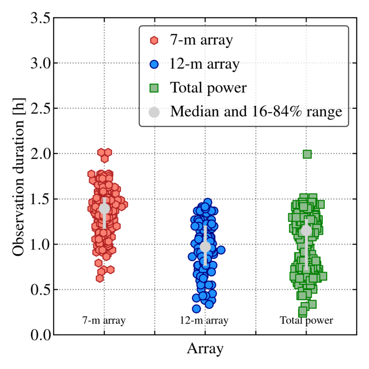


Figure 23 visualizes the conditions of our individual observations, which are also summarized in Table 14 and reported in detail in Tables 11, 12, and 13. In brief, individual observations typically lasted h across all arrays, and most observations took place at mean elevation of with precipitable water vapor (PWV) mm. The tables and figures report more exact numbers, but overall this reflects almost ideal scheduling on behalf of the array. The high elevation imply limited shadowing, and minimal atmospheric contamination, and the PWV of the observations is almost always less than the mm associated with ALMA’s 5th octile of weather conditions, the nominal threshold for 230 GHz (Band 6) observations.
V.2.3 Achieved coverage and synthesized beam

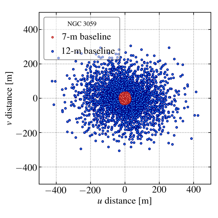


Tables 13 through 14 report the minimum, maximum, and median baseline length of each observation. We visualize this in Figure 24, which shows these values for each observation. On average, the 12-m baselines span m with median baseline length m. In terms of wavelength, this translates to a range of k, corresponding to , with a mean of k, corresponding to . The 7-m data typically span baselines m with a mean of m. This maps to k, corresponding to , with a mean of k, corresponding to . Figure 24 shows that there is some scatter in the median 12-m baseline length across our data, and significant, about , scatter in the maximum baseline for the 12-m data. However, the 7-m coverage remains stable, consistent with the fixed positions of the ACA, and in all cases there is good overlap between the 12-m baseline range, the 7-m baseline range, and the diameter of the total power antennas.
The baseline range only gives the approximate response of the array. Figures 25, 26, and 27 show the coverage, distribution of collecting area vs. baseline distance, and achieved synthesized beam in more detail. All of these figures focus on one example galaxy, NGC 3059, which also appears in Figure 21.
Figures 25 and 26 show the plane coverage for one 7-m pointing (red) and one 12-m pointing (blue). In Figure 25, we see that the 7-m data, which combine several distinct observations, achieve good rotation synthesis. The 12-m data do not, but the figure shows the excellent instantaneous coverage of ALMA. The 12-m baselines do an outstanding job of filling out the plane even without long enough integrations to achieve rotation synthesis. In Figure 26 we plot the same data as in Figure 25, but now showing the distribution of collecting area as a function of baseline length for individual integrations. We use collecting area as a proxy for sensitivity, assuming fixed atmospheric conditions and integration length. The figure shows a relatively even distribution of sensitivity as a function of distance, and so spatial scale, out to m. Similar to Figure 24, but now in sharper detail, we see good sensitivity to a range of spatial scales and overlap between the three types of telescopes (note that we only indicate the range of the total power data, not the collecting area).
Figure 27 shows the sampling of the coverage. Here we show the synthesized beam for a single channel in NGC 3059. This is the same target used for Figures 25 and 26, but the beams here represent the average result across the whole mosaic because CASA does not track spatial variations of the beam. We show the beam for both the 7-m array alone and the combined 12-m+7-m array.
Both beams show a reasonable Gaussian core, but the 7-m-only beam shows significantly worse positive and negative sidelobes. This is consistent with the significantly worse performance of 7-m-only imaging compared to 12-m+7-m imaging discussed by Leroy et al. 2021. Overall, the 12-m+7-m synthesized beam, which corresponds to our key data product, looks symmetric without clearly visible pathologies in the sidelobes.
V.3 Mosaic sensitivity


Figure 28 illustrates the combined primary beam response, i.e., the mosaic sensitivity, of the 7-m data and 12-m+7-m data for one channel in one ALMA data cube. The figure shows that ALMA achieves an even sensitivity across the area of the galaxy and demonstrates the Nyquist-sampled pointing spacing used by ALMA. The outer response contour indicates the typical extent of our imaging, though in a few cases we use a more stringent primary beam cutoff. This even coverage, at the few percent level, is typical of our targets, with only a few cases showing more uneven coverage due to flagging or issues with the execution of observations.
VI Data Processing

VI.1 Summary
Leroy et al. 2021 describe the reduction and data processing for PHANGS–ALMA. That paper explains our approaches to calibration, data processing, imaging, post-processing of the imaged data, short-spacing correction, data product creation, and quality assurance. It includes an overview, illustrations of each step, and detailed discussions of our motivation for each step. The accompanying CASA+python data pipeline is also publicly available1616 16 URL provided as soon as that paper is published and sent to the arxiv.. Herrera et al. 2020 describe our calibration and imaging procedure for the total power data. Given these detailed presentations elsewhere, we only summarize the procedure here.
Figure 29, reproduced exactly from Leroy et al. 2021, summarizes the overall workflow of the PHANGS–ALMA processing pipeline. For the interferometric data, we download each observation and apply the ALMA observatory pipeline calibration. Based on inspection of the data, we found that, in general, additional by-hand flagging does not appreciably improve the quality of the final data products. We also performed several checks related to the overall calibration. We found that the internal stability of the total power appears excellent, with rms scatter of from observation to observation, and that the fluxes of the secondary calibrators derived from the 7-m and 12-m array observations agree well with expectations from the ALMA calibrator database. As discussed above, we did identify a minor, net magnitude, issue regarding the overall calibration of a subset of the total power data. We expect this to be fixed in future releases of PHANGS–ALMA but at the moment this represents a “known issue.”
Next, we staged the calibrated data for imaging. This step involves continuum subtraction, spectral regridding and rebinning, and an empirical reweighting of the data. For the current release of PHANGS–ALMA, we carried out these steps in CASA version 5.6.1, though our tests showed little influence of the adopted CASA version on our final results.
We imaged the staged data using the CASA task tclean. We use a two stage deconvolution process. In the first stage, we used the “multiscale clean” (Cornwell 2008) deconvolution algorithm with no clean mask or a very extended clean mask, and we imposed a residual threshold of 4 times the rms noise in the cube. In other words, we carry out a multiscale clean and clean the image until the maximum residual, i.e., not deconvolved emission, has signal to noise of 4. Then, we construct a more restrictive clean mask based on the location of emission in the current version of the deconvolved image. Within this more restrictive clean mask, we continue deconvolving using a classic “Hogbom clean” (Högbom 1974). We run this second stage of deconvolution, stopping when the residual, i.e., not deconvolved emission, within the clean mask has a peak or the amount of deconvolved emission changes by a negligible amount over successive calls to clean. In practice, the signal-to-noise criterion is essentially always reached.
After imaging, we correct the image cube for the response of the primary beam. The image products often have elliptical synthesized beams at arbitrary position angles. We convolve these so that the final images have a round, Gaussian synthesized beam shape. For galaxies observed in multiple separate parts by several different Science Goals, we image the data separately and then combine the different parts via a noise-weighted linear mosaicking operation at this stage. Before doing this, we smooth all of the parts of a galaxy to share a common synthesized beam. At this stage, each galaxy has a single deconvolved, primary beam-corrected interferometric image cube with a round synthesized beam.
Next, we combine the total power and interferometric data using the CASA implementation of the “feather” algorithm (Cotton 2017, e.g., see). Feathering combines the total power and interferometer data in the Fourier domain, ensuring that in the final image the low-spatial-frequency information, that is crucial to determine the overall flux of the image, is set by the total power data. Before this stage, we calibrate, baseline subtract, and image the total power data following the procedures described in Herrera et al. 2020 and Leroy et al. 2021. For a subset of galaxies, this processing included additional steps to deal with the terrestrial ozone contamination described above.
At this stage, we have our final data cubes, which we convert from units of Jy beam-1 to units of Kelvin. We use these to construct a series of data products for use in scientific analysis. First, we convolve the cubes to a series of fixed physical and angular resolutions, which allows the whole sample to be subject to rigorous comparative analysis. The exact suite of resolutions has varied over time. For the current release we create cubes with FWHM synthesize beams of , , , and , as well as pc, pc, pc, pc, pc, pc, and kpc. When convolving to fixed physical resolution, we take into account the distance to the galaxy as compiled by Anand et al. 2021, discussed in Section IV.2, and reported in Table 3.
For each cube at each resolution, we construct a three dimensional noise model, bootstrapped from regions of the cube that contain little or no signal. Then, we combine the noise models and the data cubes to construct a series of masks that identify the likely location of real CO emission inside each cube. We construct two sets of masks, high confidence “strict” masks and high completeness “broad” masks. The strict masks are constructed for each cube at each resolution. Following Rosolowsky & Leroy 2006 and Leroy et al. 2021, these strict masks initially consider only locations in the cube where emission exceeds signal-to-noise of over two consecutive velocity channels. Then, we extend these masks to include any adjacent regions where the emission exceeds a signal-to-noise of over two consecutive velocity channels. We refer to these strict masks as “high confidence” because this construction procedure renders them very likely to include mostly real emission. The broad masks are created from the union of strict masks across all resolutions. These masks aim for “high completeness” in the sense that they tend to include almost all emission in the cube, as determined by comparison to the integrated flux from the total power data.
Finally, we apply the masks to the cubes and noise models and “collapse” the cubes to produce a series of two-dimensional maps and associated uncertainty maps. We discuss the specific products more below, but briefly these “moment maps” include images of integrated intensity, peak intensity along the line of sight, intensity-weighted mean velocity, and the spectral width of the CO line along the line of sight. We produce an associated uncertainty map for each moment map.
For more details on each step of this process see Leroy et al. 2021 and the associated, public PHANGS–ALMA post-processing pipeline.
VI.2 Validation, known issues, and limitations
We engaged in a mixture of automated and manual quality assurance of the data and validation of the PHANGS–ALMA pipeline. A broad cross-section of the team participated in several rounds of manual inspection, looking at the cubes, associated imaging products, and derived data products. For each version of the data after early 2019, we ran automated regression tests to quantify changes from version to version and to ensure that we understood the reason for all changes. Finally, to validate our pipeline, we carried out end-to-end tests using the ALMA simulator in CASA. These tests allowed us to verify that the pipeline output represents a close match to the known input to the simulator.
These tests, and other checks, showed that our data processing has yielded stable results over time, that the results pass manual inspections by experts, and that the output from the pipeline replicates known input to good precision. However, there are still several known limitations of our approach and issues related to data processing that we note here.
- 1.
Both the spectral and angular resolution of the data could be improved at the cost of signal-to-noise. The convolution to a round beam and matching beams between parts of multi-part mosaics both somewhat inflate the synthesized beam size. We also use a weighting scheme with intermediate “robustness parameter.” All of these choices improve the surface brightness sensitivity, but they degrade the resolution by a modest amount. Our cubes also use a km s-1 channel width, which is coarser than the native spectral resolution. By altering these choices, future processing of the data could improve the spatial and spectral resolution at the cost of signal-to-noise. This may be of particular interest for bright regions like the centers of galaxies.
- 2.
Deconvolution of 7-m-only imaging depends sensitively on the signal-to-noise and structure of the data. Both our real data and end-to-end tests based on simulations show that the image reconstruction performs poorly using low or moderate signal-to-noise data from the 7-m array alone. The effect is explored in detail in Leroy et al. 2021, and it is largely alleviated by short-spacing correction. However, the 7-m-only data for many galaxies appear unreliable. We also view the combined 7-m and total power data as less reliable than the full combined 12-m, 7-m, and total power data.
- 3.
There is a small known bias in the total power flux calibration. As mentioned above and discussed in Leroy et al. 2021, there was a small lag incorporating upgrades to the surface accuracy of the total power antennas into the observatory-provided calibration. As a result, a subset of our total power data sets apply an observatory-provided calibration known to be high by . The net effect is that a subset of cubes has overall fluxes biased high by . This will be fixed in future releases.
- 4.
The data processing introduces some mild dependence of noise on frequency. As discussed in Leroy et al. 2021, the regridding and rebinning parts of the staging procedure introduce a mild spectral variation into the noise of the final data cubes. The overall magnitude is across the full bandwidth of the cubes. The effect seems unavoidable in the current version of CASA, but we expect this to be addressed in the future.
Several other issues arose during processing that we have largely addressed, including the telluric ozone contamination of the total power data. To our knowledge the issues above represent the main outstanding issues and limitations of the data.
VII Data properties and key products
| Quantity | Value |
|---|---|
| Targets | |
| … 12-m+7-m+TP | 81 |
| … 12-m+7-m+TP, pcaaWe adopt a tolerance when convolving to a fixed physical resolution, so that all maps with pc have “150 pc” data products. | 78 |
| … 7-m+TP or 7-m | 9 |
| … 7-m+TP or 7-m, pcaaWe adopt a tolerance when convolving to a fixed physical resolution, so that all maps with pc have “150 pc” data products. | 7 |
| Properties of 12-m+7-m+TP data… | median (min–max) |
| Resolution… | |
| … angular [″] | () |
| … physical [pc] | () |
| noise in the cube … | |
| … mJy beam-1 native res. | () |
| … mK native res. | () |
| … mK at pc res. | () |
| … massb,cb,cfootnotemark: native res. [ M⊙] | () |
| … massb,cb,cfootnotemark: at pc res. [ M⊙] | () |
| Implied surface brightness noiseccWhen calculating line-integrated quantities, including mass and surface brightness, we adopt a full line width of km s-1. This implies an improvement of in the surface brightness sensitivity. … | |
| … K km s-1 native res. | () |
| … K km s-1 at 150 pc res. | () |
| … b,cb,cfootnotemark: native res. [M⊙ pc-2] | () |
| … massb,cb,cfootnotemark: at 150 pc res. [M⊙ pc-2] | () |
| Completenessdd“Completeness” is defined here as the ratio of the sum of flux in the strictly masked moment 0 map to the direct sum of the whole cube or the broad map. Completeness is not random but correlates with the overall brightness of the galaxy. See §VII.1.2. … | |
| … at native resolution | (%) |
| … at 150 pc resolution | (%) |
| Area mapped | |
| Physical area | |
| … total for survey [kpc2] | 10,650 |
| … mean 12-m+7-m+TP [kpc2] | 124 |
| … mean 7-m+TP [kpc2] | 71 |
| Angular area | |
| … total for survey [arcmin2] | 1,050 |
| … mean 12-m+7-m+TP [arcmin2] | 7.0 |
| … mean 7-m+TP [arcmin2] | 54 |
VII.1 Properties of the final cubes
| Galaxy | Arrays | Resolution | Area Mapped | Noise | Completeness | Notes | |||||
|---|---|---|---|---|---|---|---|---|---|---|---|
| Angular | Physical | Angular | Physical | Natve | 150 pc | Natve | Native | 150 pc | |||
| (′′) | (pc) | (arcmin2) | (kpc2) | (mK) | (mK) | (%) | (%) | ||||
| NGC 0247 | 7m+TP | ||||||||||
| NGC 0253 | 7m+TP | ||||||||||
| NGC 0300 | 7m+TP | ||||||||||
| NGC 0628 | 12m+7m+TP | ||||||||||
| NGC 0685 | 12m+7m+TP | ||||||||||
| NGC 1068 | 7m+TP | ||||||||||
| NGC 1097 | 12m+7m+TP | ||||||||||
| NGC 1087 | 12m+7m+TP | ||||||||||
| NGC 1313 | 7m | ||||||||||
| NGC 1300 | 12m+7m+TP | ||||||||||
| NGC 1317 | 12m+7m+TP | ||||||||||
| IC 1954 | 12m+7m+TP | ||||||||||
| NGC 1365 | 12m+7m+TP | ||||||||||
| NGC 1385 | 12m+7m+TP | ||||||||||
| NGC 1433 | 12m+7m+TP | ||||||||||
| NGC 1511 | 12m+7m+TP | ||||||||||
| NGC 1512 | 12m+7m+TP | ||||||||||
| NGC 1546 | 12m+7m+TP | ||||||||||
| NGC 1559 | 12m+7m+TP | ||||||||||
| NGC 1566 | 12m+7m+TP | ||||||||||
| NGC 1637 | 12m+7m+TP | ||||||||||
| NGC 1672 | 12m+7m+TP | ||||||||||
| NGC 1809 | 12m+7m+TP | FFFaint galaxy, completeness is unreliable. See text. | FFFaint galaxy, completeness is unreliable. See text. | ||||||||
| NGC 1792 | 12m+7m+TP | ||||||||||
| NGC 2090 | 12m+7m+TP | ||||||||||
| NGC 2283 | 12m+7m+TP | ||||||||||
| NGC 2566 | 12m+7m+TP | ||||||||||
| NGC 2775 | 12m+7m+TP | ||||||||||
| NGC 2835 | 12m+7m+TP | ||||||||||
| NGC 2903 | 12m+7m+TP | ||||||||||
| NGC 2997 | 12m+7m+TP | ||||||||||
| NGC 3059 | 12m+7m+TP | ||||||||||
| NGC 3137 | 12m+7m+TP | ||||||||||
| NGC 3239 | 12m+7m+TP | FFFaint galaxy, completeness is unreliable. See text. | FFFaint galaxy, completeness is unreliable. See text. | ||||||||
| NGC 3351 | 12m+7m+TP | ||||||||||
| NGC 3489 | 12m+7m+TP | FFFaint galaxy, completeness is unreliable. See text. | FFFaint galaxy, completeness is unreliable. See text. | ||||||||
| NGC 3511 | 12m+7m+TP | ||||||||||
| NGC 3507 | 12m+7m+TP | ||||||||||
| NGC 3521 | 12m+7m+TP | ||||||||||
| NGC 3596 | 12m+7m+TP | ||||||||||
| NGC 3599 | 12m+7m+TP | FFFaint galaxy, completeness is unreliable. See text. | FFFaint galaxy, completeness is unreliable. See text. | ||||||||
| NGC 3621 | 12m+7m+TP | ||||||||||
| NGC 3626 | 12m+7m+TP | FFFaint galaxy, completeness is unreliable. See text. | FFFaint galaxy, completeness is unreliable. See text. | ||||||||
| NGC 3627 | 12m+7m+TP | ||||||||||
| NGC 4207 | 12m+7m+TP | ||||||||||
| NGC 4254 | 12m+7m+TP | ||||||||||
| NGC 4293 | 12m+7m+TP | ||||||||||
| NGC 4298 | 12m+7m+TP | ||||||||||
| NGC 4303 | 12m+7m+TP | ||||||||||
| NGC 4321 | 12m+7m+TP | ||||||||||
| NGC 4424 | 12m+7m+TP | ||||||||||
| NGC 4457 | 12m+7m+TP | ||||||||||
| NGC 4459 | 12m+7m+TP | FFFaint galaxy, completeness is unreliable. See text. | FFFaint galaxy, completeness is unreliable. See text. | ||||||||
| NGC 4476 | 12m+7m+TP | FFFaint galaxy, completeness is unreliable. See text. | FFFaint galaxy, completeness is unreliable. See text. | ||||||||
| NGC 4477 | 12m+7m+TP | FFFaint galaxy, completeness is unreliable. See text. | FFFaint galaxy, completeness is unreliable. See text. | ||||||||
| NGC 4496A | 12m+7m+TP | ||||||||||
| NGC 4535 | 12m+7m+TP | ||||||||||
| NGC 4536 | 12m+7m+TP | ||||||||||
| NGC 4540 | 12m+7m+TP | ||||||||||
| NGC 4548 | 12m+7m+TP | ||||||||||
| NGC 4569 | 12m+7m+TP | ||||||||||
| NGC 4571 | 12m+7m+TP | ||||||||||
| NGC 4579 | 12m+7m+TP | ||||||||||
| NGC 4596 | 12m+7m+TP | FFFaint galaxy, completeness is unreliable. See text. | FFFaint galaxy, completeness is unreliable. See text. | ||||||||
| NGC 4654 | 12m+7m+TP | ||||||||||
| NGC 4689 | 12m+7m+TP | ||||||||||
| NGC 4694 | 12m+7m+TP | FFFaint galaxy, completeness is unreliable. See text. | FFFaint galaxy, completeness is unreliable. See text. | ||||||||
| NGC 4731 | 12m+7m+TP | FFFaint galaxy, completeness is unreliable. See text. | FFFaint galaxy, completeness is unreliable. See text. | ||||||||
| NGC 4781 | 12m+7m+TP | ||||||||||
| NGC 4826 | 12m+7m+TP | ||||||||||
| NGC 4941 | 12m+7m+TP | ||||||||||
| NGC 4951 | 12m+7m+TP | ||||||||||
| NGC 4945 | 7m+TP | ||||||||||
| NGC 5042 | 12m+7m+TP | ||||||||||
| NGC 5068 | 12m+7m+TP | ||||||||||
| NGC 5134 | 12m+7m+TP | ||||||||||
| NGC 5128 | 7m+TP | ||||||||||
| NGC 5236 | 12m+7m+TP | ||||||||||
| NGC 5248 | 12m+7m+TP | ||||||||||
| CIRCINUS | 7m+TP | ||||||||||
| NGC 5530 | 12m+7m+TP | ||||||||||
| NGC 5643 | 12m+7m+TP | ||||||||||
| NGC 6300 | 12m+7m+TP | ||||||||||
| NGC 6744 | 12m+7m+TP | ||||||||||
| IC 5273 | 12m+7m+TP | ||||||||||
| NGC 7456 | 12m+7m+TP | FFFaint galaxy, completeness is unreliable. See text. | FFFaint galaxy, completeness is unreliable. See text. | ||||||||
| NGC 7496 | 12m+7m+TP | ||||||||||
| IC 5332 | 12m+7m+TP | FFFaint galaxy, completeness is unreliable. See text. | FFFaint galaxy, completeness is unreliable. See text. | ||||||||
| NGC 7743 | 12m+7m+TP | FFFaint galaxy, completeness is unreliable. See text. | FFFaint galaxy, completeness is unreliable. See text. | ||||||||
| NGC 7793 | 7m+TP | ||||||||||
Note. — Properties of the PHANGS–ALMA data cubes. Columns — name of the galaxy; best available array combination; physical and angular resolution of the native resolution cube; noise in surface brightness (mK) units at the native resolution and pc resolution, if available; noise in mJy beam-1 units in the native-resoltion cube; completeness, defined as the ratio of flux inside the strict mask to the sum of the cube or the broad mask. See text. at native resolution and 150 pc resolution.

Table 15 summarizes the properties of our final cubes, which we report in detail in Table 16. For each target, we note the best available array combination, angular and physical resolution, noise, and completeness. When translating angular to physical beam size and coverage area, we use the distances reported in Table 3 and compiled by Anand et al. 2021. The reported noise represents the median value in the three dimensional noise cube, and should be characteristic for the cube. Here we define completeness, , as
| (12) |
that is, the ratio of flux inside the “strict,” high confidence, high signal-to-noise based mask to the total flux in the cube. The “max” in the denominator uses the larger of the sum inside the “broad” mask or the cube; we adopt this to help account for some instability in the direct sum of cubes with faint CO emission (see below). Thus, the completeness, , represents the fraction of the total flux recovered at good signal-to-noise.
Figure 30 and Table 15 summarize the area mapped. In total, PHANGS–ALMA surveyed arcmin2, slightly larger than the angular size of the Moon. At the distances to our targets, this translates to kpc2. On average, the individual maps cover kpc2 for the 12-m+7-m+TP and kpc2 for 7-m+TP data. This corresponds to linear map sizes of kpc or typical coverage out to kpc. Because the 7-m-only targets tend to lie much closer, they cover on average 54 arcmin2, compared to arcmin2, on average for the 12-m+7-m data.
VII.1.1 Resolution


Figure 31 and Table 15 summarize the resolutions reported in Table 16. For our 12-m+7-m+TP data sets, the median angular resolution is with of the data between . At the distance to our targets, this translates to a median physical resolution of pc with of the data between pc and pc. The top left panel in Figure 31 shows that most of the 7-m-only data sets target very nearby galaxies, Mpc. As a result, they achieve similar physical resolutions to the 12-m+7-m+TP observations of our more distant sample members, with a typical resolution of pc for these very nearby galaxies. The lone large-distance 7-m-only data set is NGC 1068, which has not yet been mapped in CO() using the 12-m array (García-Burillo et al. 2014, but has been mapped in CO() using ALMA by).
We construct data products at a series of fixed physical resolutions, in addition to the native angular resolution and several coarser angular resolutions. For the 12-m+7-m data we adopt FWHM beam size , , , and pc at the distance to the galaxy. Reflecting uncertainties in the distance determination, we allow a tolerance when labeling a galaxy as having that resolution; that is, we label a map with pc or pc as a “100 pc” resolution map. The bottom right panel of Figure 31 and Table 15 show the motivation for these choices: of our 12-m+7-m galaxies and of 7-m-only galaxies have pc, allowing us to construct a “ pc resolution” map. Meanwhile, roughly half of our targets have physical resolution better than pc and have physical resolution better than pc.
VII.1.2 Sensitivity


Figure 32 and Table 15 summarize the sensitivity of our data. The top left panel in Figure 32 shows the point source sensitivity in Jy beam-1 units as a function of the distance to the source. In that panel, we plot two lines showing the cases where the noise and distance equate to mass sensitivity of and M⊙ for a line width of km s-1. As above, we translate from line flux to molecular mass via:
| (13) |
where is the line-integrated CO() flux in Jy km s-1 of a source at distance. Again is the CO-to-H2 conversion factor and is the CO()-to-CO() line ratio in Kelvins, so that refers to the thermal case. For reference, if the flux is instead in units of K km s-1 arcsec2, the mass can be calculated via
| (14) |
where now is the line-integrated CO() flux in units of K km s-1 arcsec2.
Note that when converting our sensitivity into mass units, e.g., in Figure 32 and Table 15, we assume a fiducial line width of km s-1 for the line but we measure the initial noise in km s-1 channels. Noise in Jy beam-1 improves by due to averaging before calculating with the noise in Jy beam-1 averaged across the line.
The table and figure show that our typical rms point source sensitivity is mJy beam-1 per km s-1 channel, about times better than our minimum sensitivity of mJy beam-1 per km s-1 channel (see §V.1). This is partially due to the convolutions during our post-processing, but mostly reflecting that our observations typically achieve s per pointing, which translates to min of effective integration time after accounting for overlap of mosaic fields. There is about rms scatter in the point source sensitivity across our sample.
Our achieved sensitivity translates to a median point mass sensitivity of M⊙ for a Galactic and . As discussed above, this means that, on average, we will detect individual GMCs, which are often defined to have mass M⊙, at signal-to-noise of or higher.
Our median surface brightness sensitivity is mK per km s-1 channel, again better than the nominal target of mK per km s-1 channel. This surface brightness sensitivity depends sharply on the achieved angular resolution, with rms noise even for fixed point source sensitivity. This number thus partially also reflects that our achieved median resolution is while the target was . Because the surface brightness sensitivity depends on both point source sensitivity and achieved angular resolution, our data show a scatter about the median value.
Again assuming a full line width km s-1, this mK per km s-1 channel translates to surface brightness sensitivity of K km s-1. Following Equation 11, this translates to median mass surface density sensitivity of M⊙ pc-2. As discussed above, typical resolved GMCs have surface densities of a few times M⊙ pc-2. Thus our maps should recover CO emission everywhere where GMCs fill an appreciable fraction of the beam.
As discussed above, pc is a common physical scale for most of the data. When we convolve to this scale, the typical surface brightness sensitivity is mK, again with scatter. The corresponding point mass sensitivity is M⊙, and the mass surface density sensitivity is M⊙ pc-2.
Together these sensitivity numbers can all be roughly summarized as: the PHANGS–ALMA CO maps are sensitive to individual massive giant molecular clouds at the level. This has been key to the already published studies of Sun et al. 2018; Sun et al. 2020b and Rosolowsky et al. 2021, which have used PHANGS–ALMA to study populations of individual clouds across our sample.
VII.1.3 Completeness
Table 15 and Figure 33 illustrate the completeness, , of the data. Following Equation 12, we define “completeness” as the ratio of the flux detected within the “strict” mask to the total flux in the cube, estimated from either a direct sum or using the “broad” mask. This completeness thus measures how much of the flux in the cube is detected at moderate signal to noise at a given sensitivity and resolution. Figure 33 shows completeness for the native resolution and Tables 15 and 16 also report values at pc resolution.
At our native resolution, the 12-m+7-m+TP data have median completeness of , but with a wide range. This improves to at 150 pc resolution, but still shows a wide range. Figure 33 shows that the completeness variations track the overall flux of the target, with brighter galaxies yielding higher recovery. A few of the galaxies are so faint that a simple sum of the cube no longer yields a flux consistent with integrating over the broad, high completeness map. This typically occurs when K km s-1 arcsec2. We mark this regime in Figure 33 and note galaxies that have flux lower than this in Table 16. To avoid instability when calculating , we use the maximum flux of either the direct sum of the cube or the broad map in Equation 12.
Excluding these “faint” galaxies increases the median completeness in the sample by , but Figure 33 shows that there is still a trend with brightness at higher flux: we detect of the flux at native resolution in high-flux galaxies. Meanwhile for galaxies with intermediate integrated fluxes, the completeness varies across almost the whole range of possible values, but is lower on average.
Overall these levels of flux recovery are very good, and in line with previous measurements on Local Group and related data by Leroy et al. 2016 and previous measurements in PHANGS–ALMA by Sun et al. 2018; Sun et al. 2020b. The completeness increases dramatically as we degrade the resolution of the data, with almost all area in PHANGS–ALMA detected at or kpc resolution (recall that this is expected because PHANGS–ALMA targets regions with detectable mid-IR dust emission).
Note that Sun et al. 2020b give equations for the selection function associated with our strict masking technique. These can be useful for modeling the properties of the emission not included in the strict mask.
VII.2 Description of high level data products
Leroy et al. 2021 describe the creation of the PHANGS–ALMA data products, and we refer the reader to that paper for details. Here we provide a high level summary of the products that make up the PHANGS–ALMA data release:
- 1.
Cubes at multiple resolutions. We convolve the native resolution, post-processed data cubes to a series of common physical and angular resolutions. In addition to the native resolution, we convolve all data to angular resolutions of , , , and (FWHM). Almost all of the 12-m+7-m data can reach each of these angular resolutions, while the 7-m-only data sets can typically only reach and .
We also convolve each cube to a FWHM resolution corresponding to , , , , , , and pc using the distances compiled by Anand et al. 2021 and reported in Table 3. As discussed above the first four values roughly correspond to the quartiles of the distribution of physical resolutions for our native resolution 12-m+7-m data set.
During these convolutions we impose a tolerance. That is, if the FWHM beam of a cube is already within of the target resolution, we do not convolve but label the cube as belonging to that fixed-resolution subset. We do not alter the cube metadata in these cases, so that, e.g., the FITS header BMAJ and BMIN keywords still reflect the true values.
Because most scientific applications involve measuring surface brightness or integrating over an aperture larger than the beam, we present the PHANGS–ALMA cubes in units of Kelvin. Conversions to Jy beam-1 are provided as part of the header metadata.
- 2.
Noise models for each cube. For each data cube at each resolution, we construct a three dimensional noise model. This model gives our best estimate of the rms noise at each position–position–velocity pixel. We construct the noise model by treating the spectral and spatial variations of the noise as separable and then using iterative outlier rejection to isolate the parts of the cube most likely to be signal free. When discussing the noise statistics above, we quote the median value across the whole noise model, but see Leroy et al. 2021 for illustrations of the spatial and spectral variations of the noise.
- 3.
“Strict” and “broad” masks for each cube. Combining the cubes and the noise models, we construct two sets of three dimensional masks that identify the location of likely signal. Our “strict” masks are high confidence, meaning that they include only pixels with at least moderate signal to noise at the relevant resolution. The strict masks should be used in calculations that require secure detections. These are the basis of our completeness calculations above.
We also construct “broad” masks that include all regions of the cube likely to contain signal. These are high completeness masks, in the sense that we expect them to include essentially all emission from the galaxy. To build the broad masks, we use the union of the strict masks at all resolutions, from the native resolution up to and kpc. The coarse resolution masks play a crucial role here because we detect emission along almost every line of sight in those cubes. Including the high resolution masks in the union tends to matter most for high line width, compact features, which mostly occur in galaxy centers. Within the cubes, the broad masks typically look like an extended, “puffed up,” version of the galaxy rotation curve in position-position velocity space.
Because the broad mask represents a union of all strict masks, there is only a single broad mask, which we apply across all resolutions. We reproject it onto different three dimensional astrometric grids as necessary.
- 4.
Integrated intensity maps. We apply the masks to the cubes and integrate along the spectral axis to produced two-dimensional maps of line-integrated intensity (“moment 0”), in units of K km s-1. We create versions of these maps for each resolution and for both the strict and the broad masks. The “strict” integrated intensity maps should be used as our best map of securely detected CO emission from each galaxy. The “broad” integrated intensity maps represent our most complete map of CO emission from each galaxy. The broad maps will include some negative pixels, reflecting that they include regions dominated by noise but likely to contain faint emission. Integrating across these broad maps should yield the total flux in the cube to good approximation.
The integrated intensity, in units of K km s-1, can be translated into an estimate of molecular gas mass surface density, in units of M⊙ pc-2, following Equation 10 or Equation 11 for standard assumptions. At the resolution of PHANGS–ALMA it remains ambiguous whether or not to apply an inclination correction, , when estimating . There is a long history of assuming individual molecular clouds to have an isotropic, spherically symmetric geometry (Solomon et al. 1987; Rosolowsky & Leroy 2006, e.g.,). However, our resolution is of the same order as the pc disk scale height (Heyer & Dame 2015; Sun et al. 2020a). For now, the user will need to make their own best judgment on this topic.
For each integrated intensity map, we also propagate the noise model into maps of the associated statistical uncertainty in (Leroy et al. 2021, see details in).
- 5.
Peak intensity maps. We also calculate maps of the peak intensity, along each line of sight. These maps of peak intensity, also called “peak temperature” or “moment 8,” are useful to highlight the detailed structure of emission in the cube, though they have a less straightforward physical interpretation than the line-integrated intensity maps.
To calculate the peak intensity, we first calculate the full velocity range covered by the relevant mask for each sightline. Then for each line of sight, we find the maximum intensity at any velocity in this range and record this as the peak intensity.
We also create a version of the peak intensity map after convolving the spectral axis of the cube with a 12.5 km s-1 boxcar kernel. Because km s-1 corresponds to a typical full line width for a bright molecular cloud, this spectral smoothing essentially represents running a matched filter across the spectral axis.
We present the peak intensity maps in units of Kelvin.
- 6.
Velocity fields. We calculate the intensity-weighted mean velocity of emission, frequently referred to as “moment 1,” along each line of sight.
We present two versions of the intensity-weighted mean velocity field. The first uses only emission within the strict mask. These strictly masked velocity maps present the mean velocity associated with all securely detected emission.
The second set of velocity maps consider more emission and so cover a larger area. Because noise spikes can contribute spurious outliers to the velocity field, we apply several prior expectations when constructing this velocity field. These “moment 1 with prior” maps begin with the broad mask. We calculate the intensity-weighted mean velocity using the broad masks. This typically includes many spurious velocities associated with low signal-to-noise or even signal-free regions. Therefore, we blank all values from the map that either (1) have signal to noise less than two in the integrated intensity map or (2) deviate from a “prior expectation” velocity field by more than some tolerance, km s-1 by default. For this release, we use the velocity field calculated using the strict mask at lower resolution.
We present all velocity fields in units of km s-1 and also calculate maps of associated statistical uncertainty by propagating errors from the noise model cubes.
- 7.
Line width maps. We calculate two sets of line width maps, both using only the strict masks. First, we calculate the rms velocity dispersion about the intensity-weighted mean velocity, often referred to as “moment 2.” This calculation diverges in the presence of noise, so we only present the calculation for the strictly masked case.
The second moment can be sensitive to clipping and unstable in the presence of noise. We also calculate and report the “effective width” following the definition of Heyer et al. 2001 and discussed in Leroy et al. 2016 and Sun et al. 2018; Sun et al. 2020b. In this measurement, the line width . In other words, the line width is defined as the ratio of the line integrated intensity to the peak intensity. In the limit of a well-resolved, high signal-to-noise Gaussian line profile the two line width measurements match. The effective width is more robust to the presence of noise but also sensitive to the requirement to resolve the line. The ratio between the two line width measurements can also indicate deviations from a single Gaussian spectral shape.
For both line width estimates, we present the result in units of km s-1 and also calculate and deliver associated maps of statistical uncertainty. For this delivery, we do not correct the measurements for the line spread function. This can be an important effect for narrow lines and should be addressed by the user (Leroy et al. 2016; Koch et al. 2018; Sun et al. 2020a; Rosolowsky et al. 2021, e.g., following).
This already represents a rich set of data products that characterize the CO spectral line position-by-position across each target. We also provide several supporting data products, including maps indicating the coverage of the ALMA observations. There are also several clear next steps. In the inner regions of galaxies and in regions of colliding flows (Bešlić et al. 2021, e.g., bar ends, see), multi-component decomposition like that presented in Henshaw et al. 2020 represents a better treatment of the spectrum than single component methods. In the future, we also intend to use the rotation curves fit in Lang et al. 2020 to refine the “priors” use to construct the velocity fields (Colombo et al. 2014b, e.g., see). Our next round of products will also likely include “shuffled” cubes appropriate for spectral stacking (Schruba et al. 2011, e.g., see).
VIII Atlas

Fig. SetA. Atlas of PHANGS–ALMA maps.
A figure set in the online version of this paper presents an atlas of data products for the PHANGS–ALMA targets, which we illustrate with an example in Figure 34. For each galaxy, we illustrate the area mapped by ALMA over the DSS optical image of the galaxy (top left). Then we show four ALMA data products:
- 1.
The peak intensity map calculated over a 12.5 km s-1 window (top right) highlights detailed structure of each galaxy. Arms, bars, filamentary structure, and individual cloud complexes are all highly visible in these maps. Because the maps show the maximum over the full velocity extent of the mask, these offer a direct view of the contents of the data cubes.
- 2.
The integrated intensity map (middle left) on a logarithmic stretch shows the distribution of CO (2-1) emission in the galaxy. Here we show the integrated intensity map constructed using the “broad”, i.e., high completeness, mask. Therefore these maps show almost all emission from the galaxy, though note that we do set the lower end of the color stretch to 1 K km s-1, cloud to our nominal limit (see Table 15).
- 3.
A map of line width (middle right) on a logarithmic stretch. In the atlas, we show line widths calculated using the effective width. Because the line width is challenging to calculate in the presence of noise, these maps use the “strict”, i.e., high confidence, masks.
- 4.
The velocity field appears in the bottom left panel. We show the “moment 1 with prior”, i.e., the intensity-weighted mean velocity calculated within the broad, high completeness mask and then pruned using a low resolution prior estimate of the velocity. This represents our velocity field with the highest covering fraction and illustrates both large and small-scale systematic motions in the galaxy.
Along with these images, each figure notes a few key properties of each galaxy along with the best available array combination.
IX Summary
This paper presents PHANGS–ALMA, the first large pc resolution CO() survey of a representative nearby galaxy population. The paper describes:
- 1.
The scientific motivation for PHANGS–ALMA (§II). We summarize how PHANGS–ALMA builds on previous CO mapping efforts in the local universe, highlight that many key physics related to both star formation and galaxy evolution occur at or near the scale of individual giant molecular clouds (GMCs), and outline the high-level science goals of PHANGS–ALMA:
Measure the demographics of molecular clouds, and measure how GMC populations depend on host galaxy and location in a galaxy.
Measure the star formation efficiency per free fall time, , at cloud scales. Measure how depends on the density, dynamical state, and turbulence in molecular clouds.
Quantify the “violent cycling” between phases of the star formation process. Use this to constrain the life cycle of clouds and feedback.
Measure how the self-regulated, large scale structure of galaxy disks emerges from a medium made of individual clouds and star-forming regions.
Measure the motions, flows, and organization of cold gas in galaxies at pc scales.
- 2.
The sample selection (§III). PHANGS–ALMA attempts to target all relatively massive, actively star-forming galaxies within Mpc that are not heavily inclined. This means that the sample selection is unbiased, easy to understand, and simple to attempt to reproduce. It also means that a secondary goal of PHANGS–ALMA is that ALMA provide a high quality CO map of all local galaxies. Our estimates of key galaxy properties, including distance and stellar mass, have evolved some since the original sample selection. We show that while uncertainties in galaxy properties do affect our exact sample, we include approximately the expected number of targets. We also show that the targets do a good job of spanning the main sequence of star-forming galaxies and the mass radius relation for late-type galaxies.
- 3.
Calculation and presentation of the properties of the sample galaxies (§IV). We present estimates the physical properties of the PHANGS–ALMA targets: size, mass, CO luminosity, and star formation rate (SFR). We draw distances from the recent work by Anand et al. 2021. We compare estimates of these quantities using different methods and provide quantitative translations between different methods of estimating size, mass, and SFR. This includes new work on the size and stellar mass estimation.
We attempt to present numbers on a system that is self-consistent with work on the SDSS main galaxy sample by Salim et al. 2016 and Salim et al. 2018, which is itself broadly consistent with earlier work on the SDSS main galaxy sample. To verify this overall consistency, we show a good agreement between the properties of the PHANGS–ALMA targets and previous measurements of the main sequence of star-forming galaxies and the mass-radius relation.
PHANGS–ALMA typically covers only of the star formation activity, and so presumably missed of the molecular gas. To account for this, we provide aperture corrections that can be used to correct the measured CO luminosity to the full CO luminosity for comparison to other global properties or unresolved CO surveys. We consider several aperture correction templates, including an exponential disk model and several bands. We find that WISE3 m emission provides the best template for such an aperture correction, in good agreement with recent work by Chown et al. 2021.
- 4.
A summary of the PHANGS–ALMA observations (§V). We observe the area of active star formation, as gauged from mid-infrared (WISE m) emission. To cover this area, we use large mosaics. In many cases where the galaxy exceeds the area covered by a single pointing mosaic we break a galaxy into parts and observe each part separately, combining the data into a single cube in post-processing. The observations spanned years and the typical elevation and atmospheric conditions were excellent, and mm of precipitable water vapor. Even though the total observing time on any given field using the 12-m array was short, the achieve coverage for the combined 12-m+7-m data appears excellent and yields a synthesized beam without dramatic sidelobe features.
- 5.
A short summary of the data processing (§VI). We provide a short overview of the PHANGS–ALMA post-processing and product creation pipeline. The full pipeline is presented in Leroy et al. 2021 and will be publicly available along with the PHANGS–ALMA data products.
- 6.
A description of the properties of the PHANGS–ALMA cubes and data products (§VII). We cover targets with the combined 12-m, 7-m, and total power arrays and targets with the 7-m array or combined 7-m plus total power arrays. A typical 12-m+7-m+TP map covers arcmin2 or kpc2. In total, the survey maps arcmin2 or kpc2.
For the 12-m+7-m+TP data, the median angular resolution is , the channel width is km s-1, and the typical sensitivity is mJy beam-1 or 85 mK. These values translate to a median physical resolution of pc and sensitivity to mass of M⊙ for typical Milky Way conditions. Across almost the whole survey, pc represents a common physical resolution achievable for most data. At the native resolution, our cubes recover a median of the total flux in the noise at good signal to noise.
- 7.
An atlas showing the data for each target (§VIII). A figure set shows the areal coverage, peak and integrated intensity, velocity field, and line width maps for each galaxy.
ADS/JAO.ALMA#2012.1.00650.S, ADS/JAO.ALMA#2013.1.00803.S, ADS/JAO.ALMA#2013.1.01161.S, ADS/JAO.ALMA#2015.1.00121.S, ADS/JAO.ALMA#2015.1.00782.S, ADS/JAO.ALMA#2015.1.00925.S, ADS/JAO.ALMA#2015.1.00956.S, ADS/JAO.ALMA#2016.1.00386.S, ADS/JAO.ALMA#2017.1.00392.S, ADS/JAO.ALMA#2017.1.00766.S, ADS/JAO.ALMA#2017.1.00886.L, ADS/JAO.ALMA#2018.1.00484.S, ADS/JAO.ALMA#2018.1.01321.S, ADS/JAO.ALMA#2018.1.01651.S, ADS/JAO.ALMA#2018.A.00062.S, ADS/JAO.ALMA#2019.1.01235.S, ADS/JAO.ALMA#2019.2.00129.S, ALMA is a partnership of ESO (representing its member states), NSF (USA), and NINS (Japan), together with NRC (Canada), NSC and ASIAA (Taiwan), and KASI (Republic of Korea), in cooperation with the Republic of Chile. The Joint ALMA Observatory is operated by ESO, AUI/NRAO, and NAOJ. The National Radio Astronomy Observatory is a facility of the National Science Foundation operated under cooperative agreement by Associated Universities, Inc.
References
- Agertz et al. (2013) Agertz, O., Kravtsov, A. V., Leitner, S. N., & Gnedin, N. Y. 2013, ApJ, 770, 25
- Alatalo et al. (2013) Alatalo, K., Davis, T. A., Bureau, M., et al. 2013, MNRAS, 432, 1796
- Anand et al. (2021) Anand, G. S., Lee, J. C., Van Dyk, S. D., et al. 2021, MNRAS, 501, 3621
- Armus et al. (2009) Armus, L., Mazzarella, J. M., Evans, A. S., et al. 2009, PASP, 121, 559
- Astropy Collaboration et al. (2013) Astropy Collaboration, Robitaille, T. P., Tollerud, E. J., et al. 2013, A&A, 558, A33
- Astropy Collaboration et al. (2018) Astropy Collaboration, Price-Whelan, A. M., Sipőcz, B. M., et al. 2018, AJ, 156, 123
- Baldry et al. (2008) Baldry, I. K., Glazebrook, K., & Driver, S. P. 2008, MNRAS, 388, 945
- Barbarino et al. (2015) Barbarino, C., Dall’Ora, M., Botticella, M. T., et al. 2015, MNRAS, 448, 2312
- Bell & de Jong (2001) Bell, E. F., & de Jong, R. S. 2001, ApJ, 550, 212
- Bell et al. (2003) Bell, E. F., McIntosh, D. H., Katz, N., & Weinberg, M. D. 2003, ApJS, 149, 289
- Bešlić et al. (2021) Bešlić, I., Barnes, A. T., Bigiel, F., et al. 2021, MNRAS submitted
- Bigiel et al. (2008) Bigiel, F., Leroy, A., Walter, F., et al. 2008, AJ, 136, 2846
- Blanton & Moustakas (2009) Blanton, M. R., & Moustakas, J. 2009, ARA&A, 47, 159
- Blitz (1993) Blitz, L. 1993, in Protostars and Planets III, ed. E. H. Levy & J. I. Lunine, 125–161
- Blitz et al. (2007) Blitz, L., Fukui, Y., Kawamura, A., et al. 2007, in Protostars and Planets V, ed. B. Reipurth, D. Jewitt, & K. Keil, 81–96
- Blitz & Rosolowsky (2006) Blitz, L., & Rosolowsky, E. 2006, ApJ, 650, 933
- Boissier et al. (2003) Boissier, S., Prantzos, N., Boselli, A., & Gavazzi, G. 2003, MNRAS, 346, 1215
- Bolatto et al. (2008) Bolatto, A. D., Leroy, A. K., Rosolowsky, E., Walter, F., & Blitz, L. 2008, ApJ, 686, 948
- Bolatto et al. (2013a) Bolatto, A. D., Wolfire, M., & Leroy, A. K. 2013a, ARA&A, 51, 207
- Bolatto et al. (2013b) Bolatto, A. D., Warren, S. R., Leroy, A. K., et al. 2013b, Nature, 499, 450
- Bolatto et al. (2017) Bolatto, A. D., Wong, T., Utomo, D., et al. 2017, ApJ, 846, 159
- Boquien et al. (2019) Boquien, M., Burgarella, D., Roehlly, Y., et al. 2019, A&A, 622, A103
- Boquien et al. (2016) Boquien, M., Kennicutt, R., Calzetti, D., et al. 2016, A&A, 591, A6
- Bothwell et al. (2014) Bothwell, M. S., Wagg, J., Cicone, C., et al. 2014, MNRAS, 445, 2599
- Braine & Combes (1992) Braine, J., & Combes, F. 1992, A&A, 264, 433
- Braine et al. (2007) Braine, J., Ferguson, A. M. N., Bertoldi, F., & Wilson, C. D. 2007, ApJ, 669, L73
- Braine et al. (2018) Braine, J., Rosolowsky, E., Gratier, P., Corbelli, E., & Schuster, K. F. 2018, A&A, 612, A51
- Brownson et al. (2020) Brownson, S., Belfiore, F., Maiolino, R., Lin, L., & Carniani, S. 2020, MNRAS, 498, L66
- Bruzual & Charlot (2003) Bruzual, G., & Charlot, S. 2003, MNRAS, 344, 1000
- Burkhart (2018) Burkhart, B. 2018, ApJ, 863, 118
- Caldú-Primo & Schruba (2016) Caldú-Primo, A., & Schruba, A. 2016, AJ, 151, 34
- Calzetti (2013) Calzetti, D. 2013, in Secular Evolution of Galaxies, ed. J. Falcón-Barroso & J. H. Knapen, 419
- Calzetti et al. (2005) Calzetti, D., Kennicutt, Jr., R. C., Bianchi, L., et al. 2005, ApJ, 633, 871
- Cardelli et al. (1989) Cardelli, J. A., Clayton, G. C., & Mathis, J. S. 1989, ApJ, 345, 245
- Catinella et al. (2018) Catinella, B., Saintonge, A., Janowiecki, S., et al. 2018, MNRAS, 476, 875
- Chabrier (2003) Chabrier, G. 2003, PASP, 115, 763
- Chastenet et al. (2019) Chastenet, J., Sandstrom, K., Chiang, I. D., et al. 2019, ApJ, 876, 62
- Chevance et al. (2020a) Chevance, M., Kruijssen, J. M. D., Krumholz, M. R., et al. 2020a, arXiv e-prints, arXiv:2010.13788
- Chevance et al. (2020b) Chevance, M., Kruijssen, J. M. D., Hygate, A. P. S., et al. 2020b, MNRAS, 493, 2872
- Chevance et al. (2020c) Chevance, M., Kruijssen, J. M. D., Vazquez-Semadeni, E., et al. 2020c, Space Sci. Rev., 216, 50
- Chown et al. (2021) Chown, R., Li, C., Parker, L., et al. 2021, MNRAS, 500, 1261
- Colombo et al. (2014a) Colombo, D., Hughes, A., Schinnerer, E., et al. 2014a, ApJ, 784, 3
- Colombo et al. (2014b) Colombo, D., Meidt, S. E., Schinnerer, E., et al. 2014b, ApJ, 784, 4
- Colombo et al. (2018) Colombo, D., Kalinova, V., Utomo, D., et al. 2018, MNRAS, 475, 1791
- Corbelli et al. (2017) Corbelli, E., Braine, J., Bandiera, R., et al. 2017, A&A, 601, A146
- Corder et al. (2008) Corder, S., Sheth, K., Scoville, N. Z., et al. 2008, ApJ, 689, 148
- Cormier et al. (2018) Cormier, D., Bigiel, F., Jiménez-Donaire, M. J., et al. 2018, MNRAS, 475, 3909
- Cornwell (2008) Cornwell, T. J. 2008, IEEE Journal of Selected Topics in Signal Processing, 2, 793
- Cotton (2017) Cotton, W. D. 2017, PASP, 129, 094501
- Courtois & Tully (2012) Courtois, H. M., & Tully, R. B. 2012, ApJ, 749, 174
- Dale et al. (2020) Dale, D. A., Anderson, K. R., Bran, L. M., et al. 2020, AJ, 159, 195
- Dale (2015) Dale, J. E. 2015, New A Rev., 68, 1
- Davis et al. (2014) Davis, S. W., Jiang, Y.-F., Stone, J. M., & Murray, N. 2014, ApJ, 796, 107
- Davis & McDermid (2017) Davis, T. A., & McDermid, R. M. 2017, MNRAS, 464, 453
- de Vaucouleurs et al. (1991) de Vaucouleurs, G., de Vaucouleurs, A., Corwin, Herold G., J., et al. 1991, Third Reference Catalogue of Bright Galaxies (New York: Springer)
- den Brok et al. (2021) den Brok, J. S., Chatzigiannakis, D., Bigiel, F., et al. 2021, MNRAS submitted
- Dobbs et al. (2019) Dobbs, C. L., Rosolowsky, E., Pettitt, A. R., et al. 2019, MNRAS, 485, 4997
- Dobbs et al. (2014) Dobbs, C. L., Krumholz, M. R., Ballesteros-Paredes, J., et al. 2014, in Protostars and Planets VI, ed. H. Beuther, R. S. Klessen, C. P. Dullemond, & T. Henning, 3
- Donovan Meyer et al. (2012) Donovan Meyer, J., Koda, J., Momose, R., et al. 2012, ApJ, 744, 42
- Donovan Meyer et al. (2013) —. 2013, ApJ, 772, 107
- Downes & Solomon (1998) Downes, D., & Solomon, P. M. 1998, ApJ, 507, 615
- Druard et al. (2014) Druard, C., Braine, J., Schuster, K. F., et al. 2014, A&A, 567, A118
- Egusa et al. (2017) Egusa, F., Mentuch Cooper, E., Koda, J., & Baba, J. 2017, MNRAS, 465, 460
- Elmegreen (1989) Elmegreen, B. G. 1989, ApJ, 338, 178
- Elmegreen (2000) —. 2000, ApJ, 530, 277
- Elmegreen et al. (2018) Elmegreen, B. G., Elmegreen, D. M., & Efremov, Y. N. 2018, ApJ, 863, 59
- Engargiola et al. (2003) Engargiola, G., Plambeck, R. L., Rosolowsky, E., & Blitz, L. 2003, ApJS, 149, 343
- Engelbracht et al. (2006) Engelbracht, C. W., Kundurthy, P., Gordon, K. D., et al. 2006, ApJ, 642, L127
- Espada et al. (2019) Espada, D., Verley, S., Miura, R. E., et al. 2019, ApJ, 887, 88
- Evans et al. (2014) Evans, II, N. J., Heiderman, A., & Vutisalchavakul, N. 2014, ApJ, 782, 114
- Faesi et al. (2018) Faesi, C. M., Lada, C. J., & Forbrich, J. 2018, ApJ, 857, 19
- Federrath & Klessen (2012) Federrath, C., & Klessen, R. S. 2012, ApJ, 761, 156
- Federrath & Klessen (2013) —. 2013, ApJ, 763, 51
- Federrath et al. (2010) Federrath, C., Roman-Duval, J., Klessen, R. S., Schmidt, W., & Mac Low, M. M. 2010, A&A, 512, A81
- Foyle et al. (2010) Foyle, K., Rix, H.-W., Walter, F., & Leroy, A. K. 2010, ApJ, 725, 534
- Freedman et al. (2001) Freedman, W. L., Madore, B. F., Gibson, B. K., et al. 2001, ApJ, 553, 47
- Freeman et al. (2017) Freeman, P., Rosolowsky, E., Kruijssen, J. M. D., Bastian, N., & Adamo, A. 2017, MNRAS, 468, 1769
- Fukui et al. (2020) Fukui, Y., Habe, A., Inoue, T., Enokiya, R., & Tachihara, K. 2020, PASJ, arXiv:2009.05077
- Fukui & Kawamura (2010) Fukui, Y., & Kawamura, A. 2010, ARA&A, 48, 547
- Fukui et al. (1999) Fukui, Y., Mizuno, N., Yamaguchi, R., et al. 1999, PASJ, 51, 745
- Fukui et al. (2008) Fukui, Y., Kawamura, A., Minamidani, T., et al. 2008, ApJS, 178, 56
- García-Burillo et al. (2003) García-Burillo, S., Combes, F., Hunt, L. K., et al. 2003, A&A, 407, 485
- García-Burillo et al. (2014) García-Burillo, S., Combes, F., Usero, A., et al. 2014, A&A, 567, A125
- Gatto et al. (2015) Gatto, A., Walch, S., Low, M. M. M., et al. 2015, MNRAS, 449, 1057
- Geen et al. (2021) Geen, S., Bieri, R., Rosdahl, J., & de Koter, A. 2021, MNRAS, 501, 1352
- Geen et al. (2016) Geen, S., Hennebelle, P., Tremblin, P., & Rosdahl, J. 2016, MNRAS, 463, 3129
- Gentry et al. (2017) Gentry, E. S., Krumholz, M. R., Dekel, A., & Madau, P. 2017, MNRAS, 465, 2471
- Ginsburg et al. (2019) Ginsburg, A., Koch, E., Robitaille, T., et al. 2019, radio-astro-tools/spectral-cube: Release v0.4.5, doi:10.5281/zenodo.3558614
- Grasha et al. (2018) Grasha, K., Calzetti, D., Bittle, L., et al. 2018, MNRAS, 481, 1016
- Gratier et al. (2010) Gratier, P., Braine, J., Rodriguez-Fernandez, N. J., et al. 2010, A&A, 512, A68+
- Gratier et al. (2012) —. 2012, A&A, 542, A108
- Groves et al. (2012) Groves, B., Krause, O., Sandstrom, K., et al. 2012, MNRAS, 426, 892
- Grudić et al. (2020) Grudić, M. Y., Kruijssen, J. M. D., Faucher-Giguère, C.-A., et al. 2020, arXiv e-prints, arXiv:2008.04453
- Hartmann et al. (2001a) Hartmann, L., Ballesteros-Paredes, J., & Bergin, E. A. 2001a, ApJ, 562, 852
- Hartmann et al. (2001b) —. 2001b, ApJ, 562, 852
- Helfer et al. (2003) Helfer, T. T., Thornley, M. D., Regan, M. W., et al. 2003, ApJS, 145, 259
- Hennebelle & Chabrier (2011) Hennebelle, P., & Chabrier, G. 2011, ApJ, 743, L29
- Henshaw et al. (2020) Henshaw, J. D., Kruijssen, J. M. D., Longmore, S. N., et al. 2020, Nature Astronomy, 4, 1064
- Herrera et al. (2020) Herrera, C. N., Pety, J., Hughes, A., et al. 2020, A&A, 634, A121
- Heyer & Dame (2015) Heyer, M., & Dame, T. M. 2015, ARA&A, 53, 583
- Heyer et al. (2001) Heyer, M. H., Carpenter, J. M., & Snell, R. L. 2001, ApJ, 551, 852
- Hirota et al. (2018) Hirota, A., Egusa, F., Baba, J., et al. 2018, PASJ, 70, 73
- Högbom (1974) Högbom, J. A. 1974, A&AS, 15, 417
- Hopkins (2013) Hopkins, P. F. 2013, MNRAS, 428, 1950
- Hopkins et al. (2012) Hopkins, P. F., Kereš, D., Murray, N., Quataert, E., & Hernquist, L. 2012, MNRAS, 427, 968
- Hopkins et al. (2013) Hopkins, P. F., Narayanan, D., & Murray, N. 2013, MNRAS, 432, 2647
- Huang et al. (2020) Huang, C. D., Riess, A. G., Yuan, W., et al. 2020, ApJ, 889, 5
- Huang & Kauffmann (2015) Huang, M.-L., & Kauffmann, G. 2015, MNRAS, 450, 1375
- Hughes et al. (2013a) Hughes, A., Meidt, S. E., Colombo, D., et al. 2013a, ApJ, 779, 46
- Hughes et al. (2013b) Hughes, A., Meidt, S. E., Schinnerer, E., et al. 2013b, ApJ, 779, 44
- Hunt et al. (2015) Hunt, L. K., García-Burillo, S., Casasola, V., et al. 2015, A&A, 583, A114
- Ibáñez-Mejía et al. (2016) Ibáñez-Mejía, J. C., Mac Low, M.-M., Klessen, R. S., & Baczynski, C. 2016, ApJ, 824, 41
- Inoue & Fukui (2013) Inoue, T., & Fukui, Y. 2013, ApJ, 774, L31
- Jackson et al. (2010) Jackson, J. M., Finn, S. C., Chambers, E. T., Rathborne, J. M., & Simon, R. 2010, ApJ, 719, L185
- Jameson et al. (2016) Jameson, K. E., Bolatto, A. D., Leroy, A. K., et al. 2016, ApJ, 825, 12
- Jarrett et al. (2003) Jarrett, T. H., Chester, T., Cutri, R., Schneider, S. E., & Huchra, J. P. 2003, AJ, 125, 525
- Jarrett et al. (2013) Jarrett, T. H., Masci, F., Tsai, C. W., et al. 2013, AJ, 145, 6
- Jeffreson & Kruijssen (2018) Jeffreson, S. M. R., & Kruijssen, J. M. D. 2018, MNRAS, 476, 3688
- Jeffreson et al. (2020) Jeffreson, S. M. R., Kruijssen, J. M. D., Keller, B. W., Chevance, M., & Glover, S. C. O. 2020, MNRAS, 498, 385
- Jiménez-Donaire et al. (2019) Jiménez-Donaire, M. J., Bigiel, F., Leroy, A. K., et al. 2019, ApJ, 880, 127
- Jogee et al. (2005) Jogee, S., Scoville, N., & Kenney, J. D. P. 2005, ApJ, 630, 837
- Kannappan et al. (2013) Kannappan, S. J., Stark, D. V., Eckert, K. D., et al. 2013, ApJ, 777, 42
- Karachentsev et al. (2004) Karachentsev, I. D., Karachentseva, V. E., Huchtmeier, W. K., & Makarov, D. I. 2004, AJ, 127, 2031
- Karim et al. (2011) Karim, A., Schinnerer, E., Martínez-Sansigre, A., et al. 2011, ApJ, 730, 61
- Kauffmann et al. (2003) Kauffmann, G., Heckman, T. M., White, S. D. M., et al. 2003, MNRAS, 341, 33
- Kawamura et al. (2009) Kawamura, A., Mizuno, Y., Minamidani, T., et al. 2009, ApJS, 184, 1
- Keller & Kruijssen (2020) Keller, B. W., & Kruijssen, J. M. D. 2020, arXiv e-prints, arXiv:2004.03608
- Kenney et al. (1992) Kenney, J. D. P., Wilson, C. D., Scoville, N. Z., Devereux, N. A., & Young, J. S. 1992, ApJ, 395, L79
- Kennicutt & Evans (2012) Kennicutt, R. C., & Evans, N. J. 2012, ARA&A, 50, 531
- Kennicutt (1989) Kennicutt, Jr., R. C. 1989, ApJ, 344, 685
- Kennicutt et al. (2007) Kennicutt, Jr., R. C., Calzetti, D., Walter, F., et al. 2007, ApJ, 671, 333
- Kim & Ostriker (2017) Kim, C.-G., & Ostriker, E. C. 2017, ApJ, 846, 133
- Kim et al. (2013) Kim, C.-G., Ostriker, E. C., & Kim, W.-T. 2013, ApJ, 776, 1
- Kim et al. (2020a) Kim, J., Chevance, M., Kruijssen, J. M. D., et al. 2020a, MNRAS submitted, arXiv:2012.00019
- Kim et al. (2018) Kim, J.-G., Kim, W.-T., & Ostriker, E. C. 2018, ApJ, 859, 68
- Kim et al. (2019) —. 2019, ApJ, 883, 102
- Kim et al. (2020b) Kim, J.-G., Ostriker, E. C., & Filippova, N. 2020b, arXiv e-prints, arXiv:2011.07772
- Kim et al. (2020c) Kim, W.-T., Kim, C.-G., & Ostriker, E. C. 2020c, ApJ, 898, 35
- Klessen & Glover (2016) Klessen, R. S., & Glover, S. C. O. 2016, Saas-Fee Advanced Course, 43, 85
- Koch et al. (2018) Koch, E., Rosolowsky, E., & Leroy, A. K. 2018, Research Notes of the American Astronomical Society, 2, 220
- Koch & Rosolowsky (2015) Koch, E. W., & Rosolowsky, E. W. 2015, MNRAS, 452, 3435
- Koda et al. (2009) Koda, J., Scoville, N., Sawada, T., et al. 2009, ApJ, 700, L132
- Koda et al. (2020) Koda, J., Sawada, T., Sakamoto, K., et al. 2020, ApJ, 890, L10
- Kourkchi et al. (2020) Kourkchi, E., Courtois, H. M., Graziani, R., et al. 2020, AJ, 159, 67
- Kourkchi & Tully (2017) Kourkchi, E., & Tully, R. B. 2017, ApJ, 843, 16
- Kreckel et al. (2016) Kreckel, K., Blanc, G. A., Schinnerer, E., et al. 2016, ApJ, 827, 103
- Kreckel et al. (2018) Kreckel, K., Faesi, C., Kruijssen, J. M. D., et al. 2018, ApJ, 863, L21
- Kregel et al. (2002) Kregel, M., van der Kruit, P. C., & de Grijs, R. 2002, MNRAS, 334, 646
- Kruijssen (2012) Kruijssen, J. M. D. 2012, MNRAS, 426, 3008
- Kruijssen & Longmore (2014) Kruijssen, J. M. D., & Longmore, S. N. 2014, MNRAS, 439, 3239
- Kruijssen et al. (2018) Kruijssen, J. M. D., Schruba, A., Hygate, A. e. P. S., et al. 2018, MNRAS, 479, 1866
- Kruijssen et al. (2019) Kruijssen, J. M. D., Schruba, A., Chevance, M., et al. 2019, Nature, 569, 519
- Krumholz (2014) Krumholz, M. R. 2014, Phys. Rep., 539, 49
- Krumholz & Dekel (2012) Krumholz, M. R., & Dekel, A. 2012, ApJ, 753, 16
- Krumholz & McKee (2005) Krumholz, M. R., & McKee, C. F. 2005, ApJ, 630, 250
- Krumholz & McKee (2020) —. 2020, MNRAS, 494, 624
- Krumholz et al. (2019) Krumholz, M. R., McKee, C. F., & Bland-Hawthorn, J. 2019, ARA&A, 57, 227
- Kuno et al. (2007) Kuno, N., Sato, N., Nakanishi, H., et al. 2007, PASJ, 59, 117
- La Vigne et al. (2006) La Vigne, M. A., Vogel, S. N., & Ostriker, E. C. 2006, ApJ, 650, 818
- Landsman (1993) Landsman, W. B. 1993, in Astronomical Society of the Pacific Conference Series, Vol. 52, Astronomical Data Analysis Software and Systems II, ed. R. J. Hanisch, R. J. V. Brissenden, & J. Barnes, 246
- Lang (2014) Lang, D. 2014, AJ, 147, 108
- Lang et al. (2020) Lang, P., Meidt, S. E., Rosolowsky, E., et al. 2020, ApJ, 897, 122
- Lange et al. (2015) Lange, R., Driver, S. P., Robotham, A. S. G., et al. 2015, MNRAS, 447, 2603
- Lee et al. (2016) Lee, E. J., Miville-Deschênes, M.-A., & Murray, N. W. 2016, ApJ, 833, 229
- Lee et al. (2021) Lee, J. C., Whitmore, B. C., Thilker, D. A., et al. 2021, ApJS submitted, arXiv:2101.02855
- Leonard et al. (2003) Leonard, D. C., Kanbur, S. M., Ngeow, C. C., & Tanvir, N. R. 2003, ApJ, 594, 247
- Leroy et al. (2006) Leroy, A., Bolatto, A., Walter, F., & Blitz, L. 2006, ApJ, 643, 825
- Leroy et al. (2008) Leroy, A. K., Walter, F., Brinks, E., et al. 2008, AJ, 136, 2782
- Leroy et al. (2009) Leroy, A. K., Bolatto, A., Bot, C., et al. 2009, ApJ, 702, 352
- Leroy et al. (2012) Leroy, A. K., Bigiel, F., de Blok, W. J. G., et al. 2012, ArXiv e-prints, arXiv:1202.2873
- Leroy et al. (2013a) Leroy, A. K., Lee, C., Schruba, A., et al. 2013a, ApJ, 769, L12
- Leroy et al. (2013b) Leroy, A. K., Walter, F., Sandstrom, K., et al. 2013b, AJ, 146, 19
- Leroy et al. (2016) Leroy, A. K., Hughes, A., Schruba, A., et al. 2016, ApJ, 831, 16
- Leroy et al. (2017) Leroy, A. K., Schinnerer, E., Hughes, A., et al. 2017, ApJ, 846, 71
- Leroy et al. (2019) Leroy, A. K., Sandstrom, K. M., Lang, D., et al. 2019, ApJS, 244, 24
- Leroy et al. (2021) Leroy, A. K., Hughes, A., Liu, D., et al. 2021, ApJS submitted
- Leslie et al. (2020) Leslie, S. K., Schinnerer, E., Liu, D., et al. 2020, ApJ, 899, 58
- Lin et al. (2019) Lin, L., Pan, H.-A., Ellison, S. L., et al. 2019, ApJ, 884, L33
- Lisenfeld et al. (2011) Lisenfeld, U., Espada, D., Verdes-Montenegro, L., et al. 2011, A&A, 534, A102
- Longmore et al. (2013) Longmore, S. N., Bally, J., Testi, L., et al. 2013, MNRAS, 429, 987
- Lopez et al. (2011) Lopez, L. A., Krumholz, M. R., Bolatto, A. D., Prochaska, J. X., & Ramirez-Ruiz, E. 2011, ApJ, 731, 91
- Lopez et al. (2014) Lopez, L. A., Krumholz, M. R., Bolatto, A. D., et al. 2014, ApJ, 795, 121
- Lynds (1970) Lynds, B. T. 1970, in IAU Symposium, Vol. 38, The Spiral Structure of our Galaxy, ed. W. Becker & G. I. Kontopoulos, 26
- Mac Low & Klessen (2004) Mac Low, M.-M., & Klessen, R. S. 2004, Reviews of Modern Physics, 76, 125
- Makarov et al. (2014) Makarov, D., Prugniel, P., Terekhova, N., Courtois, H., & Vauglin, I. 2014, A&A, 570, A13
- Martin & Kennicutt (2001) Martin, C. L., & Kennicutt, Robert C., J. 2001, ApJ, 555, 301
- McGaugh & Schombert (2014) McGaugh, S. S., & Schombert, J. M. 2014, AJ, 148, 77
- McKee & Ostriker (2007) McKee, C. F., & Ostriker, E. C. 2007, ARA&A, 45, 565
- McMullin et al. (2007) McMullin, J. P., Waters, B., Schiebel, D., Young, W., & Golap, K. 2007, in Astronomical Society of the Pacific Conference Series, Vol. 376, Astronomical Data Analysis Software and Systems XVI, ed. R. A. Shaw, F. Hill, & D. J. Bell, 127
- Meidt et al. (2012) Meidt, S. E., Schinnerer, E., Knapen, J. H., et al. 2012, ApJ, 744, 17
- Meidt et al. (2013) Meidt, S. E., Schinnerer, E., García-Burillo, S., et al. 2013, ApJ, 779, 45
- Meidt et al. (2014) Meidt, S. E., Schinnerer, E., van de Ven, G., et al. 2014, ApJ, 788, 144
- Meidt et al. (2015) Meidt, S. E., Hughes, A., Dobbs, C. L., et al. 2015, ApJ, 806, 72
- Meidt et al. (2018) Meidt, S. E., Leroy, A. K., Rosolowsky, E., et al. 2018, ApJ, 854, 100
- Meidt et al. (2020) Meidt, S. E., Glover, S. C. O., Kruijssen, J. M. D., et al. 2020, ApJ, 892, 73
- Milam et al. (2005) Milam, S. N., Savage, C., Brewster, M. A., Ziurys, L. M., & Wyckoff, S. 2005, ApJ, 634, 1126
- Miville-Deschênes et al. (2017) Miville-Deschênes, M.-A., Murray, N., & Lee, E. J. 2017, ApJ, 834, 57
- Mizuno et al. (2001) Mizuno, N., Rubio, M., Mizuno, A., et al. 2001, PASJ, 53, L45
- Momose et al. (2013) Momose, R., Koda, J., Kennicutt, Jr., R. C., et al. 2013, ApJ, 772, L13
- Muñoz-Mateos et al. (2015) Muñoz-Mateos, J. C., Sheth, K., Regan, M., et al. 2015, ApJS, 219, 3
- Murphy et al. (2011) Murphy, E. J., Condon, J. J., Schinnerer, E., et al. 2011, ApJ, 737, 67
- Murray (2011) Murray, N. 2011, ApJ, 729, 133
- Nieten et al. (2006) Nieten, C., Neininger, N., Guélin, M., et al. 2006, A&A, 453, 459
- Noeske et al. (2007) Noeske, K. G., Weiner, B. J., Faber, S. M., et al. 2007, ApJ, 660, L43
- Nugent et al. (2006) Nugent, P., Sullivan, M., Ellis, R., et al. 2006, ApJ, 645, 841
- Ochsendorf et al. (2017) Ochsendorf, B. B., Meixner, M., Roman-Duval, J., Rahman, M., & Evans, Neal J., I. 2017, ApJ, 841, 109
- Oliphant (2006) Oliphant, T. E. 2006, A guide to NumPy, Vol. 1 (Trelgol Publishing USA)
- Onodera et al. (2010) Onodera, S., Kuno, N., Tosaki, T., et al. 2010, ApJ, 722, L127
- Onodera et al. (2012) —. 2012, PASJ, 64, 133
- Orr et al. (2018) Orr, M. E., Hayward, C. C., Hopkins, P. F., et al. 2018, MNRAS, 478, 3653
- Ostriker et al. (2010) Ostriker, E. C., McKee, C. F., & Leroy, A. K. 2010, ApJ, 721, 975
- Padoan et al. (2012) Padoan, P., Haugbølle, T., & Nordlund, Å. 2012, ApJ, 759, L27
- Padoan et al. (2017) Padoan, P., Haugbølle, T., Nordlund, Å., & Frimann, S. 2017, ApJ, 840, 48
- Padoan & Nordlund (2002) Padoan, P., & Nordlund, Å. 2002, ApJ, 576, 870
- Padoan et al. (2016) Padoan, P., Pan, L., Haugbølle, T., & Nordlund, Å. 2016, ApJ, 822, 11
- Paturel et al. (2003) Paturel, G., Petit, C., Prugniel, P., et al. 2003, A&A, 412, 45
- Pety (2005) Pety, J. 2005, in SF2A-2005: Semaine de l’Astrophysique Francaise, ed. F. Casoli, T. Contini, J. M. Hameury, & L. Pagani, 721–722
- Pety et al. (2013) Pety, J., Schinnerer, E., Leroy, A. K., et al. 2013, ApJ, 779, 43
- Pierce et al. (1994) Pierce, M. J., Welch, D. L., McClure, R. D., et al. 1994, Nature, 371, 385
- Querejeta et al. (2015) Querejeta, M., Meidt, S. E., Schinnerer, E., et al. 2015, ApJS, 219, 5
- R Core Team (2015) R Core Team. 2015, R: A Language and Environment for Statistical Computing, R Foundation for Statistical Computing, Vienna, Austria
- Rahman et al. (2011) Rahman, N., Bolatto, A. D., Wong, T., et al. 2011, ApJ, 730, 72
- Rahman et al. (2012) Rahman, N., Bolatto, A. D., Xue, R., et al. 2012, ApJ, 745, 183
- Rahner et al. (2017) Rahner, D., Pellegrini, E. W., Glover, S. C. O., & Klessen, R. S. 2017, MNRAS, 470, 4453
- Rahner et al. (2019) —. 2019, MNRAS, 483, 2547
- Raskutti et al. (2016) Raskutti, S., Ostriker, E. C., & Skinner, M. A. 2016, ApJ, 829, 130
- Raskutti et al. (2017) —. 2017, ApJ, 850, 112
- Regan et al. (2001) Regan, M. W., Thornley, M. D., Helfer, T. T., et al. 2001, ApJ, 561, 218
- Reissl et al. (2018) Reissl, S., Klessen, R. S., Mac Low, M.-M., & Pellegrini, E. W. 2018, A&A, 611, A70
- Rice et al. (2016) Rice, T. S., Goodman, A. A., Bergin, E. A., Beaumont, C., & Dame, T. M. 2016, ApJ, 822, 52
- Roman-Duval et al. (2016) Roman-Duval, J., Heyer, M., Brunt, C. M., et al. 2016, ApJ, 818, 144
- Roman-Duval et al. (2010) Roman-Duval, J., Israel, F. P., Bolatto, A., et al. 2010, A&A, 518, L74+
- Rosolowsky (2007) Rosolowsky, E. 2007, ApJ, 654, 240
- Rosolowsky & Blitz (2005) Rosolowsky, E., & Blitz, L. 2005, ApJ, 623, 826
- Rosolowsky et al. (2003) Rosolowsky, E., Engargiola, G., Plambeck, R., & Blitz, L. 2003, ApJ, 599, 258
- Rosolowsky et al. (2007) Rosolowsky, E., Keto, E., Matsushita, S., & Willner, S. P. 2007, ApJ, 661, 830
- Rosolowsky & Leroy (2006) Rosolowsky, E., & Leroy, A. 2006, PASP, 118, 590
- Rosolowsky et al. (2021) Rosolowsky, E., Hughes, A., Leroy, A. K., et al. 2021, MNRAS accepted, arXiv:2101.04697
- Rubio et al. (2015) Rubio, M., Elmegreen, B. G., Hunter, D. A., et al. 2015, Nature, 525, 218
- Ruiz-Lapuente (1996) Ruiz-Lapuente, P. 1996, ApJ, 465, L83
- Saintonge et al. (2011) Saintonge, A., Kauffmann, G., Wang, J., et al. 2011, MNRAS, 415, 61
- Saintonge et al. (2016) Saintonge, A., Catinella, B., Cortese, L., et al. 2016, MNRAS, 462, 1749
- Saintonge et al. (2017) Saintonge, A., Catinella, B., Tacconi, L. J., et al. 2017, ApJS, 233, 22
- Saintonge et al. (2018) Saintonge, A., Wilson, C. D., Xiao, T., et al. 2018, MNRAS, 481, 3497
- Sakamoto et al. (1999) Sakamoto, K., Okumura, S. K., Ishizuki, S., & Scoville, N. Z. 1999, ApJS, 124, 403
- Salim et al. (2018) Salim, S., Boquien, M., & Lee, J. C. 2018, ApJ, 859, 11
- Salim et al. (2007) Salim, S., Rich, R. M., Charlot, S., et al. 2007, ApJS, 173, 267
- Salim et al. (2016) Salim, S., Lee, J. C., Janowiecki, S., et al. 2016, ApJS, 227, 2
- Salo et al. (2015) Salo, H., Laurikainen, E., Laine, J., et al. 2015, ApJS, 219, 4
- Sánchez et al. (2014) Sánchez, S. F., Rosales-Ortega, F. F., Iglesias-Páramo, J., et al. 2014, A&A, 563, A49
- Sanders et al. (2003) Sanders, D. B., Mazzarella, J. M., Kim, D., Surace, J. A., & Soifer, B. T. 2003, AJ, 126, 1607
- Sanders & Mirabel (1996) Sanders, D. B., & Mirabel, I. F. 1996, ARA&A, 34, 749
- Schinnerer et al. (2013) Schinnerer, E., Meidt, S. E., Pety, J., et al. 2013, ApJ, 779, 42
- Schinnerer et al. (2017) Schinnerer, E., Meidt, S. E., Colombo, D., et al. 2017, ApJ, 836, 62
- Schinnerer et al. (2019) Schinnerer, E., Hughes, A., Leroy, A., et al. 2019, ApJ, 887, 49
- Schmidt et al. (2016) Schmidt, T. M., Bigiel, F., Klessen, R. S., & de Blok, W. J. G. 2016, MNRAS, 457, 2642
- Schruba et al. (2018) Schruba, A., Bialy, S., & Sternberg, A. 2018, ApJ, 862, 110
- Schruba et al. (2019) Schruba, A., Kruijssen, J. M. D., & Leroy, A. K. 2019, ApJ, 883, 2
- Schruba et al. (2021) Schruba, A., Leroy, A. K., Bolatto, A. D., et al. 2021, ApJ to be subm
- Schruba et al. (2010) Schruba, A., Leroy, A. K., Walter, F., Sandstrom, K., & Rosolowsky, E. 2010, ApJ, 722, 1699
- Schruba et al. (2011) Schruba, A., Leroy, A. K., Walter, F., et al. 2011, AJ, 142, 37
- Schruba et al. (2012) —. 2012, AJ, 143, 138
- Schruba et al. (2017) Schruba, A., Leroy, A. K., Kruijssen, J. M. D., et al. 2017, ApJ, 835, 278
- Schuster et al. (2007) Schuster, K. F., Kramer, C., Hitschfeld, M., Garćıa-Burillo, S., & Mookerjea, B. 2007, A&A, 461, 143
- Semenov et al. (2018) Semenov, V. A., Kravtsov, A. V., & Gnedin, N. Y. 2018, ApJ, 861, 4
- Shaya et al. (2017) Shaya, E. J., Tully, R. B., Hoffman, Y., & Pomarède, D. 2017, ApJ, 850, 207
- Shen et al. (2003) Shen, S., Mo, H. J., White, S. D. M., et al. 2003, MNRAS, 343, 978
- Sheth et al. (2005) Sheth, K., Vogel, S. N., Regan, M. W., Thornley, M. D., & Teuben, P. J. 2005, ApJ, 632, 217
- Sheth et al. (2010) Sheth, K., Regan, M., Hinz, J. L., et al. 2010, PASP, 122, 1397
- Silk (1997) Silk, J. 1997, ApJ, 481, 703
- Simonian & Martini (2017) Simonian, G. V., & Martini, P. 2017, MNRAS, 464, 3920
- Solomon et al. (1987) Solomon, P. M., Rivolo, A. R., Barrett, J., & Yahil, A. 1987, ApJ, 319, 730
- Somerville & Davé (2015) Somerville, R. S., & Davé, R. 2015, ARA&A, 53, 51
- Sorai et al. (2019) Sorai, K., Kuno, N., Muraoka, K., et al. 2019, PASJ, 125
- Sun et al. (2018) Sun, J., Leroy, A. K., Schruba, A., et al. 2018, ApJ, 860, 172
- Sun et al. (2020a) Sun, J., Leroy, A. K., Ostriker, E. C., et al. 2020a, ApJ, 892, 148
- Sun et al. (2020b) Sun, J., Leroy, A. K., Schinnerer, E., et al. 2020b, ApJ, 901, L8
- Tan (2000) Tan, J. C. 2000, ApJ, 536, 173
- Telford et al. (2020) Telford, O. G., Dalcanton, J. J., Williams, B. F., et al. 2020, ApJ, 891, 32
- Thompson & Krumholz (2016) Thompson, T. A., & Krumholz, M. R. 2016, MNRAS, 455, 334
- Thompson et al. (2005) Thompson, T. A., Quataert, E., & Murray, N. 2005, ApJ, 630, 167
- Tonry et al. (2001) Tonry, J. L., Dressler, A., Blakeslee, J. P., et al. 2001, ApJ, 546, 681
- Tremonti et al. (2004) Tremonti, C. A., Heckman, T. M., Kauffmann, G., et al. 2004, ApJ, 613, 898
- Tress et al. (2020a) Tress, R. G., Smith, R. J., Sormani, M. C., et al. 2020a, MNRAS, 492, 2973
- Tress et al. (2020b) Tress, R. G., Sormani, M. C., Smith, R. J., et al. 2020b, arXiv e-prints, arXiv:2012.05919
- Tully et al. (2016) Tully, R. B., Courtois, H. M., & Sorce, J. G. 2016, AJ, 152, 50
- Tully et al. (2009) Tully, R. B., Rizzi, L., Shaya, E. J., et al. 2009, AJ, 138, 323
- Utomo et al. (2017) Utomo, D., Bolatto, A. D., Wong, T., et al. 2017, ApJ, 849, 26
- Utomo et al. (2018) Utomo, D., Sun, J., Leroy, A. K., et al. 2018, ApJ, 861, L18
- Vazdekis et al. (2016) Vazdekis, A., Koleva, M., Ricciardelli, E., Röck, B., & Falcón-Barroso, J. 2016, MNRAS, 463, 3409
- Vazquez-Semadeni (1994) Vazquez-Semadeni, E. 1994, ApJ, 423, 681
- Virtanen et al. (2020) Virtanen, P., Gommers, R., Oliphant, T. E., et al. 2020, Nature Methods, 17, 261
- Vutisalchavakul et al. (2016) Vutisalchavakul, N., Evans, II, N. J., & Heyer, M. 2016, ApJ, 831, 73
- Walch et al. (2015) Walch, S., Girichidis, P., Naab, T., et al. 2015, MNRAS, 454, 238
- Watkins et al. (2016) Watkins, A. E., Mihos, J. C., & Harding, P. 2016, ApJ, 826, 59
- Weigel et al. (2016) Weigel, A. K., Schawinski, K., & Bruderer, C. 2016, MNRAS, 459, 2150
- Wilson et al. (2012) Wilson, C. D., Warren, B. E., Israel, F. P., et al. 2012, MNRAS, 424, 3050
- Wilson & Rood (1994a) Wilson, T. L., & Rood, R. 1994a, ARA&A, 32, 191
- Wilson & Rood (1994b) —. 1994b, ARA&A, 32, 191
- Wong & Blitz (2002) Wong, T., & Blitz, L. 2002, ApJ, 569, 157
- Wong et al. (2011) Wong, T., Hughes, A., Ott, J., et al. 2011, ApJS, 197, 16
- Wong et al. (2013) Wong, T., Xue, R., Bolatto, A. D., et al. 2013, ApJ, 777, L4
- Wong et al. (2019) Wong, T., Hughes, A., Tokuda, K., et al. 2019, ApJ, 885, 50
- Wright et al. (2010) Wright, E. L., Eisenhardt, P. R. M., Mainzer, A. K., et al. 2010, AJ, 140, 1868
- Yim et al. (2020) Yim, K., Wong, T., Rand, R. J., & Schinnerer, E. 2020, MNRAS, 494, 4558
- Young et al. (1996) Young, J. S., Allen, L., Kenney, J. D. P., Lesser, A., & Rownd, B. 1996, AJ, 112, 1903
- Young & Scoville (1991) Young, J. S., & Scoville, N. Z. 1991, ARA&A, 29, 581
- Young et al. (1995) Young, J. S., Xie, S., Tacconi, L., et al. 1995, ApJS, 98, 219
- Young et al. (2011) Young, L. M., Bureau, M., Davis, T. A., et al. 2011, MNRAS, 414, 940
- Zucker et al. (2018) Zucker, C., Battersby, C., & Goodman, A. 2018, ApJ, 864, 153
- Zuckerman & Evans (1974) Zuckerman, B., & Evans, N. J., I. 1974, ApJ, 192, L149
Appendix A Contributions
The design, execution, processing, and scientific exploitation of PHANGS–ALMA was a team effort, with major contributions from many people and input from the entire team. This paper also reflects major direct and indirect contributions from many people. We summarize some of the key contributions here.
Observation Design, Data Processing, and Quality Assurance of the ALMA Data: Since 2016, observation design, quality assurance, pipeline and algorithm development, and data processing have all been organized through the “PHANGS ALMA Data Reduction” (ADR) working group. J. Pety has led this group since the beginning of the PHANGS collaboration, and the active members participating in almost all key activities and doing the core work on observations and data processing have been C. Faesi, C. Herrera, A. Hughes, D. Liu, A. Leroy, T. Saito, E. Rosolowsky, E. Schinnerer, A. Schruba, and A. Usero. The imaging and postprocessing pipeline for the interferometric data and the software to create derived products has been mostly developed by by A. Leroy, D. Liu, E. Rosolowsky, and T. Saito. For the total power data, the processing and software development have been led by C. Faesi, C. Herrera, J. Pety, and A. Usero. A. Hughes led quality assurance efforts and software development. A. Hygate and K. Sliwa also made early key contributions to a wide range of ADR efforts. A broad cross-section of the PHANGS–ALMA team also contributed to quality assurance efforts and gave excellent, frequent feedback. These included: A. Barnes, I. Beslic, M. Chevance, J. den Brok, C. Eibensteiner, C. Faesi, A. García-Rodríguez, C. Herrera, A. Hygate, M. Jimenez Donaire, J. Kim, A. Leroy, D. Liu, J. Pety, J. Puschnig, M. Querejeta, E. Rosolowsky, T. Saito, A. Sardone, E. Schinnerer, A. Schruba, J. Sun, A. Usero, D. Utomo, T. Williams. Please also note that Leroy et al. 2021 includes a more detailed description of contributions to the PHANGS–ALMA data processing and product generation pipeline.
Management of the PHANGS Collaboration: E. Schinnerer has served as the leader of the PHANGS collaboration since 2015. G. Blanc, E. Emsellem, A. Leroy, and E. Rosolowsky have acted as the PHANGS steering committee. E. Rosolowsky has served as team manager since 2018. The entire PHANGS core team provides key input and oversight to all major collaboration decisions. The core team includes: F. Bigiel, G. Blanc, E. Emsellem, A. Escala, B. Groves, A. Hughes, K. Kreckel, J.M.D. Kruijssen, J. Lee, A. Leroy, S. Meidt, M. Querejeta, J. Pety, E. Rosolowsky, P. Sanchez-Blazquez, K. Sandstrom, E. Schinnerer, A. Schruba, and A. Usero. Scientific exploitation of PHANGS–ALMA has taken place largely in the context of the “Cold ISM Structure and Its Relation to Star Formation” (Cold ISM) and “Large Scale Dynamical Processes” (Dynamics) science working groups. The “Cold ISM” group was led by A. Hughes and K. Kreckel in 2019 and C. Faesi and A. Hughes since 2020. The “Dynamics” group has been led by S. Meidt and M. Querejeta since 2019.
Calculation of Galaxy Properties: G. Anand, J. Lee, and the PHANGS–HST team led compilation of distances for the sample. A. Leroy, S. Meidt, M. Querejeta, K. Sandstrom, J. Sun, and T. Williams played active roles in the discussion and determination of stellar masses and sizes for the sample. I. Ho, A. Leroy, and T. Williams have curated or developed software for curating the master table of PHANGS target properties. E. Behrens and A. Leroy created by-hand masks for artifacts and stars in the multiwavelength data used to estimate the SFR and stellar masses. M. Querejeta played a key role in many aspects of obtaining and processing the IRAC data used for stellar mass estimation. Benchmarks against the MUSE-based galaxy property estimates relied on the hard work of the PHANGS–MUSE team, led by E. Emsellem with major contributions to SFR and M⋆ estimates by F. Belfiore, I. Pessa, and P. Sanchez Blazquez. The PHANGS sample definition and the SFR and M⋆ estimation built on work on this topic by A. Leroy, K. Sandstrom, J. Chastenet, and I. Chiang, heavily leveraging previous work by S. Salim, M. Boquien, and J. Lee.
Preparation of this Paper: A. Leroy led preparation of the text and figures in close collaboration with E. Schinnerer. Frequent heavy edits and early, repeated high level scientific input throughout were contributed by A. Hughes, E. Rosolowsky, K. Sandstrom, and A. Schruba. The survey motivation in Section II distills many years of collective scientific discussions and proposals by the team. S. Meidt and M. Querejeta provided major input on the section presenting the estimation of galaxy properties. The entire team provided multiple rounds of careful vetting. C. Faesi and A. Usero compiled the detailed log of observations for the total power data.
Observatory and Community Support: Across multiple large and small projects, PHANGS–ALMA has benefited from outstanding support from the Joint ALMA Observatory, the North American ALMA Science Center (NAASC) at the National Radio Astronomy Observatory (NRAO), and the European Southern Observatory (ESO). The Large Program was carried out with the NAASC as supporting ALMA Regional Center, and the NAASC staff, including ARC manager A. Remijan, have been incredibly responsive, helpful, and supportive with a wide range of technical issues. The ESO ALMA ARC has been similarly supportive whenever issues arose. PHANGS–ALMA built heavily on the high quality ALMA calibration pipeline (E. Humphreys et al. in preparation) and the CASA software package. We also heavily leveraged the work by the astropy collaboration and the broader scientific python community. We also acknowledge the astronomical IDL community, which was instrumental in many early parts of this work.