Electromagnetic wave transparency of X mode in strongly magnetized plasma
Abstract
An Electromagnetic (EM) pulse falling on a plasma medium from vacuum can either reflect or propagate inside the plasma depending on whether it is overdense or underdense. In a magnetised plasma, however, there are usually several pass and stop bands for the EM wave depending on the orientation of the magnetic field with respect to the propagation direction. The EM wave while propagating in a plasma can excite electrostatic disturbances in the plasma Vashistha et al. 2020; Vashistha et al. 2021. In this work Particle - In - Cell simulations have been carried out to illustrate the complete transparency of the EM wave propagation inside a strongly magnetised plasma. The external magnetic field is chosen to be perpendicular to both the wave propagation direction and the electric field of the EM wave, which is the X mode configuration. Despite the presence of charged electron and ion species the plasma medium behaves like a vacuum. The observation is understood with the help of particle drifts. It is shown that though the two particle species move under the influence of EM fields their motion does not lead to any charge or current source to alter the dispersion relation of the EM wave propagating in the medium. Furthermore, it is also shown that the stop band for EM wave in this regime shrinks to a zero width as both the resonance and cut-off points approach each other. Thus transparency to the EM radiation in such a strongly magnetised case appears to be a norm. This may have important implications in astrophysical scenarios. For instance, the plasma surrounding objects like pulsars and magnetars is often threaded with strong magnetic fields.
I Introduction
In astrophysical plasmas, a wide range of magnetic fields exist e.g. in galaxy clusters, shock formation in gamma ray bursts, magnetospheres of neutron stars Medvedev 2006; Vikhlinin et al. 2001; Vogt and Enßlin 2003; Taylor et al. 2002. Several instabilities also lead to the generation of intense magnetic field in the astrophysical plasmas e.g. magnetic field generation via kelvin-Helmholtz instability, counter-streaming electron flows etc Medvedev et al. 2006; Alves et al. 2012; Alves et al. 2014. Thus plasmas associated with astrophysical objects are often threaded with magnetic fields. These magnetic fields can be very strong in some cases. For instance, near pulsars and magnetars they could be of the order of Giga Teslas Mazur and Heyl 2011; Parent et al. 2011; Camilo et al. 2000. It is thus possible that electromagnetic wave would encounter a strongly magnetized plasma in such astrophysical scenarios.
Such scenarios involve understanding the interaction of EM waves with matter which has been covered with tremendous interest for many decades now Kaw and Dawson 1969; Dawson and Oberman 1963; Kaw 2017. The principle mechanisms in plasmas depend on EM wave frequency and plasma permittivity. Plasma permittivity can be altered by suitably choosing the plasma density and applied magnetic field. The free charges and their associated currents in the plasma medium act as sources and influence the plasma dielectric constant making it different from vacuum. Propagation of EM wave through strongly magnetized plasma sources, therefore, needs to be understood.
The issue of EM wave achieving complete transparency is important and has been considered earlier in many contexts. An attempt to achieve transparency using strong fields generated by intense laser pulse has been studied by Teychenné et al. 1998; Giulietti et al. 1997; Siminos et al. 2012; Kulagin et al. 2007; Palaniyappan et al. 2012. Total transmission was observed when laser pulse of intensity passes through plastic foil targets (Giulietti et al. 1997). This mechanism is operative when the target width is much smaller than the laser wavelength Teychenné et al. 1998. However, for thick targets, relativistic laser would lead to excitation of coherent structures and/or instabilities leading to turbulence in the systemMandal et al. 2020; Chatterjee et al. 2017.
External magnetic fields have been applied in several contexts to achieve transparency. The dressing of resonance states for RHCP( Right Hand Circularly Polarized) waves with the combination of axial and wiggler magnetic field is attempted to acquire a window of transparency in the opaque magnetized plasma for the EM wave Gad et al. 2012. Another technique to seek transparency is by employing pump electromagnetic wave to transmit the probe wave (Kawamori et al. 2012; Shvets and Wurtele 2002; Shvets et al. 2005; Hur et al. 2003). This method is analogous to a quantum mechanical phenomena known as EIT(Electromagnetically Induced Transparency). In this phenomena, an electromagnetic wave is made to propagate in an normally opaque medium in presence of powerful secondary EM wave. This is possible due to the destructive interference between several energy levels connecting the ground and excited states of the atom. This method is heavily used in non-linear optics to manipulate the energy levels of atomic states or slow down the wavesBoller et al. 1991; Fleischhauer et al. 2000; Harris 1993. In plasma, the use of pump and probe EM wave is used to make plasma transparent to RHCP wave. But this study is limited to propagation of RHCP waves along the magnetic field lines and generating an additional wiggler magnetic field is a complication from application viewpoint. More importantly these methods focus on R-wave mode where propagation is along the magnetic field, while L-wave and X-mode propagation geometries are yet to be explored.
We have carried out Particle - In - Cell simulations to study the propagation of EM wave in a strongly magnetized plasma for which both the electron and ion species are strongly magnetized. An interesting observation of complete transparency of the plasma medium is observed for the propagation of EM wave in the X mode configuration. The width of the stop band of the X mode reduces to zero and a completely transparent propagation of EM wave is observed. For X-mode, dispersion curve is given in fig.1, there are two stop bands ( , where stands for Lower Hybrid, Upper Hybrid, Left Hand Cutoff, Right Hand Cutoff respectively). Whenever laser/EM wave frequency lying on these bands is incident on plasma, it generates a shielding electric field in response to avoid penetration of EM wave inside it. The propagation of EM wave in plasma thus depends on the intensity and/or frequency of the incident EM wave. We show that when the strong external magnetic field dominates the motion of both charged species, i.e. , or it strongly magnetizes electrons but the perturbations are at faster time scales than that of ions , the electromagnetic wave propagates undisturbed inside plasma. The inequalities gives an insight to plasma in terms of anisotropy and modification in its collective behaviour that gets affected by introduction of magnetic field. Such caveats are vital for absorption phenomena as well.
A strong magnetic field in which the two charged species remain closely tied to the magnetic field at the EM wave frequency,
ensures that they do not provide the plasma a chance to respond to the incoming laser/ EM wave. We show that as the strength of magnetic field increases, the magnitude of self generated fields in bulk plasma due to interaction of laser with plasma decreases and the EM wave propagation speed inside the plasma approaches the speed of light . The plasma medium thus acts
as a transparent to the incoming EM wave.
These observations would have important implications in astrophysics. For instance, the strength of magnetic field in neutron stars and magnetars goes upto Giga-Tesla where this study is expected to be applicable.
The paper has been arranged as follows: Section II describes our PIC simulation, Section III contains the analysis and the discussion under different sub-sections and Sec.IV provides concluding remarks.
II Simulation Details
| criteria I () | criteria II () | (in ) | |||
|---|---|---|---|---|---|
| Region I (0-) | 3, 8 | 20 | 0.05 | 0.6 | 0.03 |
| Region II () | 3, 8 | 20, 40 | 0.2 | 0.15 | 0.03 |
| Region III () | (0.25,0.5 ),3, 8 | 40 | 0.5 | 0.06 | 0.03 |
We have carried out series of one dimensional (along ) PIC simulations in X-mode configurations using OSIRIS-4.0 Hemker 2000; Fonseca et al. 2002; Fonseca et al. 2008. For X-mode configuration, uniform external magnetic field() has been applied in direction. A uniform plasma density comprising of electrons and ions has been considered. Ion mass is taken to be 100 times mass of electrons () for faster computation. Plasma boundary extends from to whereas total length of simulation box is . Boundary condition for particles as well as fields are absorbing. A p-polarized, plane laser pulse is incident normally at plasma from the left boundary. Laser is propagating along with its spatial profile centered at x= and ranging from x= to . We also want to clarify that this work focuses on proof of concept so the mechanism presented in this paper depends on the magnetisation of the charge species with respect to the incoming EM pulse frequency. We have carried out a parametric study on magnetic fields such that broadly they follow either criteria I () or criteria II (). This parametric study has been done with laser pulse of intensity lying in non-relativistic regime such that amplitude of laser electric field() is constant for all runs. This has been done to avoid other relativistic mechanism to play a role. A schematic of simulation geometry has been shown in Fig.2. Different laser frequency maintaining criteria I and criteria II has also been chosen according to regional frequency which is explained more elaborately in next section. A tabular form of simulation parameters is given in table I.
III Results
III.1 Theory and Analytical assessment
It is well known that when EM wave is propagating perpendicular to external magnetic field, plasma supports two kinds of waves, O-mode (ordinary wave) and extraordinary mode (X-mode). O-mode is independent of applied magnetic field (ordinary wave). The general dispersion relation for perpendicular propagation in cold plasma () is given by the matrix,
| (1) |
where, , ,
| (2) |
| (3) |
The X-mode has R and L mode having cut-offs at and respectively. and are given as follows:
| (4) |
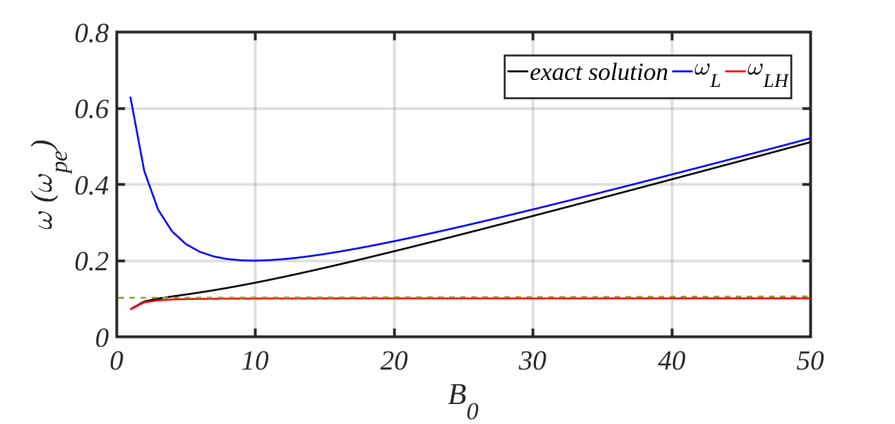
Dispersion curve of X-mode is shown in fig.1. We have classified dipersion curve into three regions depending on the dominant role played by the species. Region I is dominated by dynamics of ions and Region III for electrons. Region II is stop band as it lies between (resonance point) and (cut-off point).
Dispersion relation for X-mode is obtained
| (5) |
Principal resonance occur when
| (6) |
This is a bi-quadratic equation, it’s lower end solution is plotted as function of applied magnetic field in fig.4. As can be seen from the figure, when (at ) it falls in criteria I and solution of eq. 6 matches perfectly with reduced expression of . At higher magnetic fields, saturates at while solution of eq. 6 approaches left hand cut off ( ) asymptotically which concludes that at this higher magnetic field the resonance point and cut off approach each other thus effectively reduce the width of the stop band. This was checked by simulation as well for frequency parameter lying in region II(i.e. stop band). Under criteria I, laser reflected back. On the other hand, under criteria II laser pulse was able to propagate through the plasma. This was possible due to effective reduction of stop band and resonance point lying well above EM frequency. So, effectively this case does not lie in region II but in region I.
In Fig.3, we have plotted the dispersion curve for X-mode in two criteria. As one can observe from the left subplot that in criteria I, all the regions are well separated while in the criteria II stop band has shrunk. Moreover, the dispersion follows (as ). Therefore, it rules out any other mode excitation when .
To summarize our propagation characteristics according to their region of dispersion curve in fig. 1. is given in table II.
| criteria I | criteria II | |
|---|---|---|
| Region I | LH | Transparent |
| Region II | Stop band | Transparent |
| Region III | Transparent | N.A |
Detail quantitative analysis to calculate absorption, reflection, transmission coefficients has also been done which is presented here in tabulated form (Table III).
| R | T | A | ||
|---|---|---|---|---|
| Region I | 3 | 0.67 | 8.9 | 0.32 |
| 8 | 0.0663 | 0.872 | 0.0246 | |
| 20 | 0.0035 | 0.9931 | 0.02 | |
| Region II | 3 | 0.99 | 7.95 | 1.9 |
| 8 | 0.998 | 0.0036 | ||
| 20 | 0.0089 | 0.9823 | 0.0047 | |
| 40 | 5.6 | 0.9989 | 0.0018 | |
| Region III | 3 | 0.013 | 0.9742 | 0.003 |
| 8 | 0.006 | 0.9988 | 0.0019 | |
| 40 | 0.0035 | 0.9931 | 0.02 |
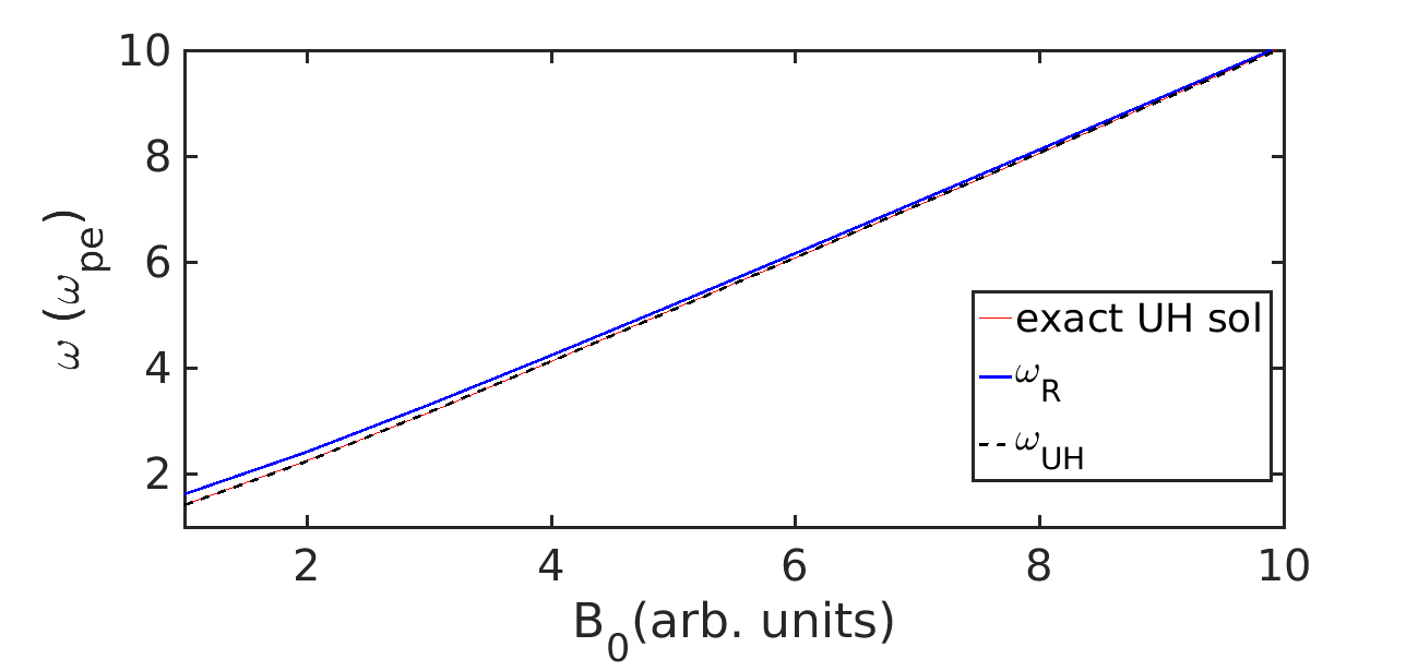
One comment should be made here about another solution in the upper end of frequency scale, it was found that at high magnetic field region dominates all modes and cut off points and hence they merge very well. Plot of exact solution of eq.6 as function of applied is given in fig.5. As one can observe here gap between and is very thin and at high magnetic fields they also merge indicating that stop band at upper frequency also vanishes with application of strong magnetic field.
III.2 and Analysis
In any dispersive medium, as the refractive index of media change spatially, the frequency of the EM wave remains same while its wavelength suffers a change. In this section we calculate the modified and the phase velocity of incident laser pulse. We observe that by varying ambient magnetic field, phase velocity of laser pulse also changes (approaches velocity of light in vacuum,) while decreasing the perturbations in the plasma.
Fig.6 shows a comparison of all three cases lying in Region I. Initially (at t=0), electric field due to laser is present in the system. In case(A) (), the laser interacts with plasma and gets reflected back from the plasma surface. However, for case(B) (, satisfying the condition ), there are certain modes generated in plasma and as a result we observe a finite magnitude of in the system. that get generated in plasma have higher magnitude than . On the other hand, in case(C) (, satisfying the condition ), the plasma seems to be completely undisturbed by the laser as pulse freely propagates inside it without creating any perturbations in the medium and goes into vacuum space in the right side. The transparency induced in plasma on applying external magnetic field is the key observation of this work. Plasma density plots show that in case(A), plasma density at the interface is modified, on the contrary, for case(B), density perturbations are present in the bulk plasma as well. Ion density fluctuates more than electrons which propagates in longitudinal direction as can be seen at later times in fig.7. For case(C), there being density perturbations that can be seen at is due to laser field i.e. electrons and ions fluctuates with same amplitude, justifying our observation that plasma remains undisturbed via interaction with laser in this case[fig. 7].
| Velocity from method I | Modified | Velocity from method II | |
|---|---|---|---|
| 8 | 0.78 | 0.2518 | 0.79 |
| 15 | 0.87 | 0.228 | 0.88 |
| 20 | 0.92 | 0.2137 | 0.94 |
| 40 | 0.96 | 0.2030 | 0.98 |
Fig. 8 shows the FFT of of laser with respect to time for four different value of magnetic field, where transparency has been induced. It can be seen that the frequency of laser() does not change while propagating inside plasma (we show FFT of with time at two different values of x in the bulk plasma and obtain the same peak.). However, of EM wave gets modified on propagation inside plasma (figure 9). The shift from the initial value of decreases on increasing applied magnetic field. We calculate the modified velocity of EM wave in plasma by peak frequency of the wave from the FFT and modified value (method II in table 4) and found that velocity of the wave inside plasma approaches to on increasing applied magnetic field ( Table 4). In table 4, we calculate velocity by two methods. In Method I, we choose a point on the waveform and calculate the time taken by that point to cover a particular distance and method II includes calculation of velocity by modification in . So we conclude that strong magnetization can stop pulse modification while pulse waveform is propagating through plasma media.
III.3 Reversible and Irreversible exchange of energy
In this study, we observed that depending on region and criteria, the laser energy exchange is either reversible or irreversible.
As one can notice from table3, in region I criteria I there is significant absorption and this region is well explored in refVashistha et al. 2020. From these studies we know that in region I criteria I energy is dominantly coupled to ions and this coupling process is irreversible. While in region I criteria II, due to tansparency, energy transfer is observe to be reversible. As when laser is present in the plasma, electrons and ions oscillate due to oscillating electric field and when the field passes through, they come to rest.
In region II criteria I, laser reflects back due to formation of shielding fields so there’s no exchange of energy altogether. On the other hand region II criteria II is effectively Region I criteria II so there’s similar exchange of energy which is reversible.
In region III criteria I, we observe transparency and reversible exchange of energy. This is quite different from other two regions, the reason behind this is simple. As the time scales of region III are same as electrons, with electrons are strongly magnetized. So that’s why laser is not able to couple its energy into electron effectively. To couple laser energy into electron irreversibly one has to weakly magnetise the electron and that can be achieved by ensuring another inequality i.e. . When we simulated with this condition by taking , we observe absorption into electrons and about energy to ions irreversibly while of laser pulse was reflected back.
We concluded that when the species are tightly bound to external magnetic field, they are not able to take energy from EM pulse irreversibly. That’s why in region I and criteria II when both the species were tightly magnetized to external magnetic field they were unable to couple their motion to laser pulse and that’s how pulse was transparent in this medium. In region III where it is in propagating region when electrons were tightly bounded we observe transparency for similar reason. One can argue that ions are not magnetized in this condition but this region’s time scales are fast so only electron motion is important here.
III.4 Drift Velocity Comparison in Different Regions
In this section, we will provide proof on how charge species are magnetized or unmagnetized in different regimes and their analytic estimates are compared to their simulation values. Under the effect of oscillating electric field and external magnetic field, the longitudinal drift can be written by eq.7
| (7) |
Here, the suffix represents the electron and ion species respectively. Like in Criteria II, both ions and electrons are strongly magnetised and the dynamics are governed by the Lorentz force i.e. eq.7. And as longitudinal velocity is independent of mass of the species for this criteria, there’s no possibility of charge separation such that there are no shielding fields to restrict the EM pulse propagation. A comparative analysis has been done between analytical drift given in eq.7 and numerical longitudinal drift experienced by both ion and electron in subplot(B) of fig. 10 and it can be observed that there’s no velocity difference between species which results in no net charge density separation and hence EM wave is able to propagate unhindered. In Criteria I, electrons follow eq.7 while ion motion is governed by electric fields as they are unmagnetized. This is shown in subplot (A) and (C) of fig.10. We observe that they match well. When (named as Criteria 0), both species are unmagnetized and they follow the longitudinal electric field (see subplot (D) of fig.10).
IV conclusion
A detail PIC simulation has been carried out by us to show complete transparency of EM wave radiation through a plasma in the presence of strong ambient field. The strength of the magnetic field has to be strong enough to elicit magnetised response from both electron and ion species at the EM wave frequency.
The effect is understood by realising that at such strong magnetic field the the hybrid modes essentially vanish and in that regime resonance point and cut-off points approach each other resulting in reduction and eventually disappearance of the width of the stop band. Thus, the EM wave freely propagates inside the plasma medium for any choice of frequency in this particular regime. It has also been shown that the particle drifts are identical for both electron and ion species at strong magnetic field. Thus, plasma provides for no charge and current sources in the EM wave propagation. The electrostatic perturbations, ( which lead to irreversible transfer of EM wave energy to plasma) normally occur due to differential drift of the two species. In this case the drifts being identical there is no conversion to electrostatic perturbations of the EM wave.
We feel that these observations will have important significance in the context of astrophysical plasma near pulsar and magnetars where the magnetic field is quite strong and would elicit magnetised plasma response for typical EM frequencies of interest.
Acknowledgements
The authors would like to acknowledge the OSIRIS Consortium, consisting of UCLA ans IST(Lisbon, Portugal) for providing access to the OSIRIS4.0 framework which is the work supported by NSF ACI-1339893. AD would like to acknowledge her J. C. Bose fellowship grant JCB/2017/000055 and the CRG/2018/000624 grant of DST for the work. The simulations for the work described in this paper were performed on Uday, an IPR Linux cluster.
References
- Vashistha et al. (2020) A. Vashistha, D. Mandal, A. Kumar, C. Shukla, and A. Das, New Journal of Physics 22, 063023 (2020), URL https://doi.org/10.1088%2F1367-2630%2Fab8cad.
- Vashistha et al. (2021) A. Vashistha, D. Mandal, and A. Das, Nuclear Fusion 61, 026016 (2021), URL https://doi.org/10.1088/1741-4326/abcc1a.
- Medvedev (2006) M. V. Medvedev, The Astrophysical Journal 651, L9 (2006), URL https://doi.org/10.1086/509075.
- Vikhlinin et al. (2001) A. Vikhlinin, M. Markevitch, and S. S. Murray, The Astrophysical Journal 549, L47 (2001), URL https://doi.org/10.1086/319126.
- Vogt and Enßlin (2003) C. Vogt and T. A. Enßlin, A&A 412, 373 (2003), eprint astro-ph/0309441.
- Taylor et al. (2002) G. B. Taylor, A. C. Fabian, and S. W. Allen, Monthly Notices of the Royal Astronomical Society 334, 769 (2002), ISSN 0035-8711, URL https://doi.org/10.1046/j.1365-8711.2002.05555.x.
- Medvedev et al. (2006) M. V. Medvedev, L. O. Silva, and M. Kamionkowski, The Astrophysical Journal 642, L1 (2006), URL https://doi.org/10.1086/504470.
- Alves et al. (2012) E. P. Alves, T. Grismayer, S. F. Martins, F. Fiúza, R. A. Fonseca, and L. O. Silva, The Astrophysical Journal 746, L14 (2012), URL https://doi.org/10.1088/2041-8205/746/2/l14.
- Alves et al. (2014) E. P. Alves, T. Grismayer, R. A. Fonseca, and L. O. Silva, New Journal of Physics 16, 035007 (2014), URL https://doi.org/10.1088/1367-2630/16/3/035007.
- Mazur and Heyl (2011) D. Mazur and J. S. Heyl, Monthly Notices of the Royal Astronomical Society 412, 1381 (2011), ISSN 0035-8711, eprint https://academic.oup.com/mnras/article-pdf/412/2/1381/5743737/mnras0412-1381.pdf, URL https://doi.org/10.1111/j.1365-2966.2010.17995.x.
- Parent et al. (2011) D. Parent, M. Kerr, P. R. den Hartog, M. G. Baring, M. E. DeCesar, C. M. Espinoza, E. V. Gotthelf, A. K. Harding, S. Johnston, V. M. Kaspi, et al., The Astrophysical Journal 743, 170 (2011), URL https://doi.org/10.1088/0004-637x/743/2/170.
- Camilo et al. (2000) F. Camilo, V. M. Kaspi, A. G. Lyne, R. N. Manchester, J. F. Bell, N. D’Amico, N. P. F. McKay, and F. Crawford, The Astrophysical Journal 541, 367 (2000), URL https://doi.org/10.1086/309435.
- Kaw and Dawson (1969) P. K. Kaw and J. M. Dawson, The Physics of Fluids 12, 2586 (1969), eprint https://aip.scitation.org/doi/pdf/10.1063/1.1692400, URL https://aip.scitation.org/doi/abs/10.1063/1.1692400.
- Dawson and Oberman (1963) J. Dawson and C. Oberman, The Physics of Fluids 6, 394 (1963), eprint https://aip.scitation.org/doi/pdf/10.1063/1.1706745, URL https://aip.scitation.org/doi/abs/10.1063/1.1706745.
- Kaw (2017) P. K. Kaw, Rev. Mod. Plasma Phys. 1, 15970 (2017).
- Teychenné et al. (1998) D. Teychenné, A. Giulietti, D. Giulietti, and L. A. Gizzi, Phys. Rev. E 58, R1245 (1998), URL https://link.aps.org/doi/10.1103/PhysRevE.58.R1245.
- Giulietti et al. (1997) D. Giulietti, L. A. Gizzi, A. Giulietti, A. Macchi, D. Teychenné, P. Chessa, A. Rousse, G. Cheriaux, J. P. Chambaret, and G. Darpentigny, Phys. Rev. Lett. 79, 3194 (1997), URL https://link.aps.org/doi/10.1103/PhysRevLett.79.3194.
- Siminos et al. (2012) E. Siminos, M. Grech, S. Skupin, T. Schlegel, and V. T. Tikhonchuk, Phys. Rev. E 86, 056404 (2012), URL https://link.aps.org/doi/10.1103/PhysRevE.86.056404.
- Kulagin et al. (2007) V. V. Kulagin, V. A. Cherepenin, M. S. Hur, and H. Suk, Physics of Plasmas 14, 113102 (2007), eprint https://doi.org/10.1063/1.2799169, URL https://doi.org/10.1063/1.2799169.
- Palaniyappan et al. (2012) S. Palaniyappan, B. M. Hegelich, H.-C. Wu, D. Jung, D. C. Gautier, L. Yin, B. J. Albright, R. P. Johnson, T. Shimada, S. Letzring, et al., Nature Physics 8, 763 (2012).
- Mandal et al. (2020) D. Mandal, A. Vashistha, and A. Das, Journal of Plasma Physics 86, 905860606 (2020).
- Chatterjee et al. (2017) G. Chatterjee, K. M. Schoeffler, P. Kumar Singh, A. Adak, A. D. Lad, S. Sengupta, P. Kaw, L. O. Silva, A. Das, and G. R. Kumar, Nature communications 8, 15970 (2017), URL http://dx.doi.org/10.1038/ncomms15970http://10.0.4.14/ncomms15970https://www.nature.com/articles/ncomms15970{#}supplementary-information.
- Gad et al. (2012) R. Gad, J. G. Leopold, A. Fisher, D. R. Fredkin, and A. Ron, Phys. Rev. Lett. 108, 155003 (2012), URL https://link.aps.org/doi/10.1103/PhysRevLett.108.155003.
- Kawamori et al. (2012) E. Kawamori, W.-J. Syugu, T.-Y. Hsieh, S.-X. Song, and C. Z. Cheng, Phys. Rev. Lett. 108, 075003 (2012), URL https://link.aps.org/doi/10.1103/PhysRevLett.108.075003.
- Shvets and Wurtele (2002) G. Shvets and J. S. Wurtele, Phys. Rev. Lett. 89, 115003 (2002), URL https://link.aps.org/doi/10.1103/PhysRevLett.89.115003.
- Shvets et al. (2005) G. Shvets, M. Tushentsov, M. D. Tokman, and A. Kryachko, Physics of Plasmas 12, 056701 (2005), eprint https://doi.org/10.1063/1.1865053, URL https://doi.org/10.1063/1.1865053.
- Hur et al. (2003) M. S. Hur, J. S. Wurtele, and G. Shvets, Physics of Plasmas 10, 3004 (2003), eprint https://doi.org/10.1063/1.1580816, URL https://doi.org/10.1063/1.1580816.
- Boller et al. (1991) K.-J. Boller, A. Imamoğlu, and S. E. Harris, Phys. Rev. Lett. 66, 2593 (1991), URL https://link.aps.org/doi/10.1103/PhysRevLett.66.2593.
- Fleischhauer et al. (2000) M. Fleischhauer, S. Yelin, and M. Lukin, Optics Communications 179, 395 (2000), ISSN 0030-4018, URL http://www.sciencedirect.com/science/article/pii/S0030401899006793.
- Harris (1993) S. E. Harris, Phys. Rev. Lett. 70, 552 (1993), URL https://link.aps.org/doi/10.1103/PhysRevLett.70.552.
- Hemker (2000) R. G. Hemker, Thesis, University of California, Los Angeles (2000), eprint 1503.00276.
- Fonseca et al. (2002) R. A. Fonseca, L. O. Silva, F. S. Tsung, V. K. Decyk, W. Lu, C. Ren, W. B. Mori, S. Deng, S. Lee, T. Katsouleas, et al., OSIRIS: A Three-Dimensional, Fully Relativistic Particle in Cell Code for Modeling Plasma Based Accelerators (Springer Berlin Heidelberg, Berlin, Heidelberg, 2002), pp. 342–351, ISBN 978-3-540-47789-1, URL http://dx.doi.org/10.1007/3-540-47789-6_36.
- Fonseca et al. (2008) R. A. Fonseca, S. F. Martins, L. O. Silva, J. W. Tonge, F. S. Tsung, and W. B. Mori, Plasma Physics and Controlled Fusion 50, 124034 (2008), URL http://stacks.iop.org/0741-3335/50/i=12/a=124034.