Hidden symmetries, spin and charge of artificial magnetic monopolesPreprint: LA-UR-21-23554
Abstract
We discuss the non-Abelian artificial magnetic monopoles associated with -level energy crossing in quantum systems. We found that hidden symmetries reveal themselves as observables such as spin, charge and other physical degrees of freedom. We illustrated our results on concrete examples of two and three energy-level crossing. Our results can be useful for modeling of various phenomena in physical and biological systems.
Keywords:
Geometric phase, monopole, quasienergy, spinI Introduction
Recent experimental results provide evidence for the emergence of artificial magnetic monopoles in the crystal-momentum space, noncommutative quantum mechanics, the anomalous Hall effect of ferromagnetic materials, and magnetic superconductors, trapped -type atoms, anisotropic spin systems, in a Bose-Einstein condensate of degenerate dressed states, etc. In particular, these monopoles own artificial magnetic fields, making it possible to model many physical phenomena BM; Br; FNT; SR; Hal; FP; ZLS; MSN; PVMM; DGJ; RPN; NVJ; RVWC; CSPA; RRKMH.
These artificial magnetic monopoles are related to the Berry phase, and energy-level crossing B0; B1. The effective gauge field gives rise to a ‘magnetic’ monopole located at the parameter space’s degeneracy point. In the simplest case of double degeneracy with two linearly independent eigenvectors, the energy surfaces form a double cone’s sheets. In the neighborhood of the degenerate point (apex of the cones), the behavior of the system can be characterized by three parameters: Arn. Each eigenstate, , gives rise to the Berry’s connection defined by , and the curvature associated with , is the field strength of artificial magnetic monopole located at the degenerate point B0; B1; BW; BD.
In general, for a quantum-mechanical system governed by a slowly varying parameter-dependent and periodic Hamiltonian, the wavefunction gains a geometric phase, which depends on the path in parameter space. For a non-adiabatic evolution of the quantum system, Berry’s phase becomes the Aharonov-Anandan geometric phase AA. The further development of this concept for the quantum mechanical systems with degenerate eigenvalues leads to the non-Abelian geometric phases WFZA; MCA; MCA1. (For a comprehensive review, see WFSA.) With each eigenstate, a monopole is associated, which is located at the degenerate point and carries its own charge. However, the total charge equals zero. For -level energy crossing, one has monopoles with different charges. And again, the total charge equals zero.
In this paper, we show that instead of -monopoles with the different charges, -level energy crossing can be characterized by a single non-Abelian artificial monopole located at the degenerate point. The monopole has matrix-valued “charge” with values in the Lie algebra of the group . In particular, for trapped - type atom interacting with two laser beams, the monopole emerges. We show that in this case, the hidden symmetry reveals itself not as the spin of the monopole but as a rather complicated mixture of spin and charge degrees of freedom.
The structure of the paper is as follows. In Sec. II, we describe the Dirac magnetic monopole’s general properties and discuss its spin. In Sec. III, we discuss the relationship between artificial magnetic monopoles and geometric phases. We show how the isospin of the artificial magnetic monopole turns into the monopole’s spin. In Sec. IV, we discuss the properties of quasienergies and geometric phases for time-periodic quantum systems. In particular, we consider superconducting qubit interacting with resonator, and spin system driven by circularly polarized field, to illustrate our findings. In Sec V, we generalize our results for -level energy crossing. We demonstrate that in this case, a non-Abelian single fictitious magnetic monopole with a matrix-valued charge occurs. In Conclusion, we discuss our results and possible applications. Through the paper, unless stated otherwise, we use the natural units, .
II Mathematical preliminaries
A magnetic monopole, introduced by Dirac in 1931 Dir, yields a magnetic field of pointlike particle,
| (1) |
where is a charge of monopole. From the second pair of Maxwell equations it follows,
| (2) |
However, the definition implies that , that is in a contradiction with Eq. (2). This contradiction can be resolved by using a singular vector potential,
| (3) |
Here the unit vector, , determines the direction of a singular string passing from the origin of coordinates to infinity. It is easy to verify now that , where
| (4) |
is the contribution of the singular string.
The choice of the vector potential (3) is unique up to a gauge transformation. For instance, the Schwinger’s choice is Sw_1
| (5) |
and the string is propagated from to , so that
| (6) |
Using the gauge freedom in the definition of the vector potential, one can show that NF; N1a
| (7) |
where
| (8) |
with being polar angle in the plane orthogonal to . The Dirac and Schwinger vector-potentials are related as follows:
| (9) |
From rotational symmetry of the theory, it follows immediately that an arbitrary gauge transformation can be undone by rotation , . Using this fact and adapting the results of Wu2; Jac; Jac1, one can show that the compensating gauge transformation is defined by a nonintegrable phase factor,
| (10) | ||||
| (11) |
where the integral is taken along the geodesic .
The equation of motion of a non-relativistic particle of a charge and mass , moving in the field of a magnetic monopole, reads
| (12) |
where . From Eq. (12) one can deduce that
| (13) |
Here is a gauge invariant angular momentum, and
| (14) |
is a total angular momentum, with being a unit vector from to .
One can show, by making use of Eqs. (12), (14), that the motion of the charged particle is confined to a cone with axis and angle (see Fig. 1) NG; LRP; LBNZ; SHY
| (15) |
The unit vector precesses around with the angular velocity
| (16) |
The motion of the charged particle in the field of the magnetic monopole is unbounded (Fig. 1), and taking into account the conservation of the energy, one can write SHY
| (17) |
where is the minimal distance between the particle and monopole located at the origin of coordinates. The equation of orbit can be written as,
| (18) |
where .

In the framework of the quantum mechanics, a motion of charged massive non-relativistic particle in the field of a magnetic monopole is described by the Schrödinger equation
| (19) |
where the Hamiltonian is given by
| (20) |
Dirac showed that quantum mechanics is consistent with the existence of magnetic monopoles, if the quantization condition , with being integer, holds Dir.
Writing the wavefunction as and employing the spherical coordinates, we obtain for eigenvalue problem, , the following equation,
| (21) |
In a classical approach the last term in Eq.(14) usually is interpreted as a contribution of the electromagnetic field, which carries an angular momentum WHA; Gol1; Gol2,
| (22) |
A quantum-mechanical description leads to the generalization of this picture and interpretation of as a spin of the composed charge-monopole particle11 1 The notion of an intrinsic spin in the Dirac monopole problem was introduced by Goldberg Gol1; Gol2. The role of spin in the consistent theory of magnetic monopole is widely discussed in the literature, see, e.g. WHA; Gol1; Gol2; SMN; SMN1; WF; WF1; JRRC; HPHG; SJ1; MKD; MAK..
Classical total angular momentum (14) can be recast as
| (23) |
Motivated by this classical expression, one could introduce the spin by defining the momentum operator as SJ1,
| (24) |
which yields
| (25) |
Here is a standard angular momentum operator, and obeyes usual spin commutation relations:
| (26) |
Then one can see that the gauge invariant operator leads to the following commutation relations:
| (27) |
and, thus, it is not acceptable as the angular momentum for a charged particle moving in the field of a magnetic monopole. The correct commutation relations are obtained for the total angular momentum:
| (28) |
Computation of the kinetic energy, , yields MAK
| (29) |
where
| (30) |
From (29) it follows
| (31) |
Using (31), one can look for a solution of Eq. (21) obeying
| (32) | ||||
| (33) |
Making use of these relations in Eq. (21) we obtain the radial Schrödinger equation.
Spin formulation of the theory, given by (29), leads to the canonical momentum, , which involves the non-Abelian vector potential MAK
| (34) |
The magnetic field strength now is determined by
| (35) |
The Abelian approach is recovered employing the unitary transformation MAK,
| (36) |
Under this transformation, (34) takes the form
| (37) |
For the eigenvalue of the spin operator, this yields the Dirac vector potential (3) with .
III Geometric phases and artificial magnetic monopoles
Let be the -dimensional Hilbert space and a set forms the orthonormal basis in . Using the Einstein summation convention, a given quantum state may be written as , where the repeated index . The space of rays is defined as an equivalence class of states , if , where is the complex constant. Thus, the space of rays being the projective Hilbert space is isomorphic to the complex projective space . The normalized states belong to the unit sphere . Indeed, the normaliztion condition implies , where , and . The complex projective space may be parametrized as follows: Let us assume that , then one can introduce the coordinates in as .
For an arbitrary quantum evolution , the geometric phase gained by the system on the time interval can be written as , where the total phase is , the dynamical phase being . If the trajectory is closed curve in the complex projective space , then the initial normalized state returns to itself up to a phase factor: . Then the geometric phase is given by the integral over the in the complex projective space PD:
| (38) |
where
| (39) |
is the connection one-form.
Applying the Stokes’s theorem, one can obtain
| (40) |
where the integration is performed over the surface subtended by the circuit , and is the curvature two-form
| (41) |
From the geometric point of view, the geometric phase generates the holonomy element , where denotes path ordering, with respect to the natural connection in a principal -bundle SB; Chj. The simplest illustrative example of geometric phase is a two-level system. In this case, the ray space is the Poincare sphere ; and the geometric phase space brings out to be one-half of the solid angle subtended by the closed curve in ray space.
The Aharonov-Anandan (AA) phase AA, is a particular case of the geometric phase , when the evolution of the quantum system is defined by the Schrödinger eqution,
| (42) |
Suppose that the wavefunction , being a solution of Eq. (42), satisfies the following condition
| (43) |
Let us consider a modified wavefunction
| (44) |
where is any function satisfying . Then, the total phase calculated for the time interval may be written as , where the “dynamical phase” is given by
| (45) |
and for the geometric AA phase one has AA
| (46) |
This yields the connection one-form and the curvature two-form as follows AS:
| (47) |
Geometric phase for an arbitrary quantum evolution can be obtained, also, from the total phase by subtracting the dynamical phase MMSY; MS; MS1; MS2:
| (48) |
where , and
| (49) |
For the adiabatic evolution with the periodic Hamiltonian, , the AA geometric phase reduces to the Berry phase as follows. Let be eigenstate corresponding to the eigenvalue . Then in the adiabatic approximation the geometric phase is given by B1; GW; B2
| (50) |
Here we assume that the instantaneous eigenvectors form the orthonormal basis, .
Validity of the adiabatic approximation is defined by the following condition:
| (51) |
This restriction is violated nearby the degeneracies, where the eigenvalues coalesce.
Inserting in the expression the complete basis system condition, , and employing the Schrödinger equation, , we obtain
| (52) |
It follows herefrom that the curvature diverges at the degeneracy points , where the energy levels, say and , are crossing, . For further it is of importance the following result: Chj.
III.1 Diabolical points and “magnetic” monopoles
In the typical case of double degeneracy with two linearly independent eigenvectors, the energy surfaces form the sheets of a double cone (see Fig. 2). The apex of the cones is called a “diabolical point” (DP) B0; BW. For a generic Hermitian Hamiltonian, the co-dimension of the DP is three, and therefore, it can be characterized by three parameters: Arn. The eigenstates, , give rise to the Berry’s connection defined as , and the curvature, , associated with is the field strength of ‘magnetic’ monopole located at the DP B0; B1; BW; BD. The Berry phase, , is interpreted as a holonomy associated with parallel transport along a circuit SB.

Since in the vicinity of each DP only terms related to the invariant subspace formed by the two-dimensional Jordan block make substantial contributions, the -dimensional problem becomes effectively two-dimensional (for details see Arn; KMS). This implies that there exists the map such that in the vicinity of the DP the quantum system can be described by the effective two-dimensional Hamiltonian, , where . This yields , where and
| (53) |
Thus, the geometric phase is independent of peculiarities of a quantum-mechanical system.
In what follows, we consider in detail the Berry phase associated with a generic Hamiltonian of two-level system:
| (54) |
The solution of the eigenvalue problem, , is given by , where . We choose the eigenvectors as,
where are the spherical coordinates in the parameter space. In the basis of the eigenstates the Hamiltonianan (54) reads
| (61) |
where .
As one can see, the coupling of eigenvalues and occurs at the DP, determined by the equation
| (62) |
Thus, the DP is located at the origin of coordinates in 3-dimensional parameter space, . At the DP we obtain
Inserting formulae (III.1) and (III.1) into Eq. (47), we obtain the connection one-form as,
| (68) |
where , and upper/lower sign corresponds to , respectively. The related curvature two-form reads
| (69) |
and computation of the geometric phase yields
| (70) |
where integration is performed over the contour on the sphere . Applying the Stokes theorem we obtain
| (71) |
where is a closed surface with the boundary , and is the solid angle subtended by the contour .
In the Cartesian coordinates the connection one-form and the curvature two-form can be written as,
| (72) | ||||
| (73) |
The obtained formulae describe two artificial ‘magnetic’ monopoles with the charges and . One can write the field strength of these monopoles as
| (74) |
where and .
III.2 Spin of artificial monopole from isospin
The phenomen of conversion of isopspin degrees of freedom into the spin degrees of freedom was discovered in the quantum gauge field theory, with the spontaneuosly broken isospin symmetry, in the field of magnetic monopole HPTHG; MSW; RJRC. It was demonstrated that the similar phenomenon can arise in some quantum-mechanical systems with induced non-Abelian gauge fields, when there exists isotopic-spin-degenerate energy levels LHZ; LHZ1.
For the monopole (74) we introduce an isospin assuming that the internal (isotopic) degrees of freedom are related with the energy levels crossing at the DP. Below we show that isospin contributes to the total angular momentum and acts as a spin, confirming that the monopole spin comes out from isospin.
Consider a non-Abelian gauge field with internal (isotopic) degrees of freedom: , where are the generators of isospin, being the Pauli matrices. Assuming , where is taking from Eq. (68),
| (76) |
we obtain . The associated field strength is the “magnetic” field of the monopole,
| (77) |
where . Thus, the different charges of the monopole (74), being associated with energy surfaces crossing at the DP, can be described as the monopole with isotopic degrees of freedom.
The total angular momentum, , yields the following commutation relations:
| (78) |
One can show that commutes with the Hamiltonian (61), and, thus, is conserved.
While explicitly the vector potential does not manifest itself as a rotational invariant field, it is rotationally symmetric in the sense that there exists a gauge transformation that compensates the rotational noninvariance of JR1.
Consider the following gauge transformations rotating the unit vector on the sphere :
As one can see, brings the Hamiltonian (61) to its initial form (54):
| (81) |
Here comprises the Pauli matrices. In a new gauge, after some work one obtains JR1; Hooft; PAM; AJFP
| (82) | ||||
| (83) | ||||
| (84) |
The curvature associated with the gauge field is:
| (85) |
Next, inserting (82) into Eq. (25), we obtain , where is a standard operator of the angular momentum. Thus, we find that the total angular momentum and projection of spin on direction are conserved. Quantization is performed in the unitary gauge, where is pointed in the third isospin direction:
| (86) | ||||
| (87) |
Evolution of the monopole spin is determined by the following equations of motion:
| (88) |
For the Hamiltonian (81) we obtain
| (89) |
which is equivalent to the Bloch equation.
IV Quasienergies and geometric phases for time-periodic quantum systems
IV.1 Quasienergies and monopole spin
When a quantum -level system interacts with the periodic external field, a dressed state (or quasi-particle) appears. This quasi-particle is characterized by a combination of the parameters of the system and the external field. In particular, not energy but quasienergy becomes a good quantum number RVI; BPXH. Below we will show that this quasi-particle gains additional degrees of freedom related to the artificial magnetic monopole at the DP’s vicinity. Thus, this monopole contributes to the observables, such as the quasienergy, susceptibility, and others.
Consider a time-periodic Hamiltonian with the period , such that . Let be a new variable. Then one can introduce the time-independent Floquet Hamiltonian,
| (90) |
acting in the extended Hilbert space , where is the space of square integrable functions on the circle . The extended Hilbert space is equipped by the scalar product:
Employing the Floquet theorem SHI; HGM, one can show that the solution of the Schrödinger equation can be written as,
| (91) |
where is the periodic wafefunction with the period . The quasienergies are defined from the eigenvalue problem for the Floquet Hamiltonian:
| (92) |
The total phase accumulated by the quantum system in the period is given by , and the computation of the dynamical phase,
| (93) |
yields the following result:
| (94) |
From here we obtain the geometric phase of the state as MDJ; MDJ1; MDJ2,
| (95) |
Next, one can apply the Hellmann-Feynman theorem,
| (96) | |||||
to obtain a simple formula for the geometric phase accumulated by the quantum system in the period GMPH,
| (97) |
As an illustrative example, let us consider a quantum mechanical system with double degeneracy of quasienergy occurring at the DP. Near the DP the system is characterized by three parameters, , and its dynamics can be described by effective Hamiltonian (81).
Returning back to the geometric phase of a Floquet state, we find that Eq. (95) can be recast as, , where
| (98) |
is the connection one-form, and the integral is taken over the circuit . To recover information on the monopole structure hidden in the quasienergy, we employ Eq. (83) to obtain
| (99) |
where is the monopole spin, , and is the solid angle subtended by the contour .
Suppose that the Hamiltonian of the system depends on the perturbation parameter in such a away that for adiabatic switch of interaction , where is time-independent Hamiltonian. Then the quasienergies satisfy GMPH
| (100) |
where we denote by the eigenenergies of the unperturbated Hamiltonian . From here and Eq. (97) we find that in the adiabatic limit of vanishing perturbation the geometric phase takes the trivial value of .
Let us assume that , where is ‘unperturbated’ stationary Hamiltonian and is a periodic operator. By differentiating the eigenvalue equation , one obtains the relations AK; BWB; SJH
| (101) |
Considering the perturbation parameter as the ‘field’ strength, one may introduce the generalized nonlinear susceptibility as,
| (102) |
In the limit it leads to (up to the numerical constant) widely known in the literature linear susceptibility:
Let us assume that
| (103) |
It yields the following Floquet Hamiltonian,
| (104) |
where and . The quasienergies are defined from the eigenvalue problem for the Floquet Hamiltonian:
| (105) |
We obtain
| (106) |
where is the detuning. The corresponding eigenvectors are
where are the spherical angles in the parameter space:
| (111) | ||||
| (112) | ||||
| (113) |
where and .
First, using (95), we calculate the geometric phase for the contour ,
| (114) |
where is the solid angle subtended by the contour . Taking the derivative of the quasienergy with respect to the frequency, , we obtain
| (115) | ||||
| (116) |
Comparison of these results with (70) yields
| (117) |
that is in agreement with Eq. (97).

Next, using Eqs.(97), (99) and (70), we obtain
| (118) |
From here it follows . Thus, we conclude that with the quasienergy is associated the projection of the monopole spin .
The computation of the generalized nonlinear susceptibility yields
| (119) |
In Fig. 3 we depict the nonlinear susceptibility, , as a function of and the detuning . As one can see, is the bifurcation line.
Let us assume that the perturbation switch on adiabatically, then the susceptibility takes the value or as a result of the spontaneous symmetry breaking. As a consequence, the monopole spin’s projection on the quantization axes takes the value or . Thus, an experiment with measuring nonlinear susceptibility offers the possibility of the experimental test for the monopole spin.
IV.2 Superconducting qubit interacting with a resonator
As the following illustrative example, we consider a superconducting qubit system interacting with a resonator. In the rotating wave approximation, the system is described by the Hamiltonian
| (120) |
We study the dynamics of the system under the condition of a given field approximation for the resonator. We suppose that initially the system is prepared in the pure state
| (121) |
where is a general qubit state, with being its eigenstates, and is the coherent state
| (122) |
Further it is assumed be real, that does not restrict the generality of consideration.
Assuming , one can write the time-dependent state as MDJ1
| (123) |
where
| (124) | |||
| (125) |
Here
| (126) |
and
| (127) |
As can be seen the states defined as
| (128) |
are the Floquet states. Indeed, as can be easily shown, the Floquet modes satisfies
| (129) |
where
| (130) |
is the quasienergy.
To calculate the geometric phase we apply Eq. (97) written as,
| (131) |
The computation yields
| (132) |
where .
As can be shown, the Floquet states are eigenfunctions of the both operators and ,
| (133) | |||
| (134) |
Thus, with the quasienergy is associated the projection of the monopole spin.
In semiclassical limit the corresponding Hamiltonian can be obtained from the initial one by replacing in the expression for with its mean value, , and the boson creation operator by the function . It takes the form MDJ1,
where is the effective coupling constant.
The geometric phase of (132) becomes the nonadiabatic geometric phase
| (138) |
with and . In the adiabatic limit, , it reduces to the Berry phase
| (139) |
IV.3 Spin system driven by circularly polarized field
Let us consider the spin- system driven by a circularly polarized time-periodic field. The Hamiltonian of the system we take in the form LHCH:
| (140) |
where is a magnetic momentum, and is the spin angular momentum operator. Its components obey the standard commutation relations: .
Further we restrict ourselves by consideration of the time-dependent periodic magnetic field rotating in the -plane, thus that . Introducing and , we recast the Hamiltonian of Eq.(140) as
| (141) |
To obtain the matrix representation of the Floquet Hamiltonian, we first introduce the Floquet state basis , where are eigenvectors of the operators and , so that and ().
In terms of the basis the Floquet Hamiltonian reads
| (142) |
where
| (143) |
As can be observed the infinite-dimensional Floquet Hamiltonian has a block-diagonal structure with dimension of each block being . Due the periodicity of quasi-energies only one block can be considered. We choose the central block defined by the subspace spanned by the following set of the Floquet basis . Then the Floquet Hamiltonian (IV.3) reduces to the -dimensional Hamiltonian
| (144) |
where , and is the identity operator. We set , where and .
As can be easily shown, the Floquet states are eigenfunctions of the both operators and ,
| (145) | |||
| (146) |
where . These relations, show that the monopole spin is an observable that can be measured simultaneously with the quasienergy.
The DP is defined by condition . As one can see, at the DP one has a -fold degeneracy. Applying (97), we obtain the geometric phase related with the quasienergy as . In particular, for , we obtain . This is exactly the expression for the Aharonov-Anandan geometric phase for spin- system AA. As known, in the adiabatic approximation it becomes the Berry phase.
V Further generalization
Here we consider more general case when -levels () become degenerate at some point. In this situation the emerging monopole has more complicated structure. Generally, being monopole, it has matrix-valued “charge”, and thus can not be characterized by only one quantum number CSB.
V.1 Non-Abelian monopoles
An outline of the monopoles theory being provided here is based on the review by S. Coleman CSB. Additional details can be found in the aforementioned review, and in the book SHY.
Generalization of the Abelian monopole theory on the gauge group is rather straightforward. For instance, the potential with the south-pointing string can be written as
| (147) |
where is matrix-valued “charge” with values in the Lie algebra of the group , . The potential with the north-pointing string is defined by
| (148) |
Both potentials yield the same ‘magnetic’ field,
| (149) |
The transformation is given by gauge transformation
| (150) |
The requirement to be a single-valued function leads to the quantization condition for non-Abelian monopole:
| (151) |
Since , it must be traceless Hermitian -matrix, which can be diagonalized, so that one can obtain
| (152) |
where . The quantization condition implies that all ’s are integers.
If the gauge group is not but , then the quantization condition is modified as follows CSID
| (153) |
where the matrix denotes the generator in the -dimensional fundamental representation of the group . From here it follows
| (154) |
However, now one has
| (155) |
where is an integer, and as before .
V.2 Trapped -type atom and monopoles
One possible way to implement a non-Abelian monopole is by employing atom-light interaction of atoms with degenerate internal degrees of freedom coupled to spatially varying laser fields OKBM; RJF; LHY; LXLX.
To illustrate these ideas, we consider a system of trapped -type atoms interacting with two laser beams, as schematically shown in Fig. 4 ZLS. (For details, we refer the reader to original papers and review DGJ.).

The quantum mechanical system is governed by the Hamiltonian that in the rotating wave approximation can be written as
| (156) |
where is atom’s momentum and is the trapping potential. The coupling Hamiltonian takes the form,
| (157) |
Here and are the complex, space-dependent Rabi frequencies for the probe and control laser beams, respectively, and is the one-photon detunning.
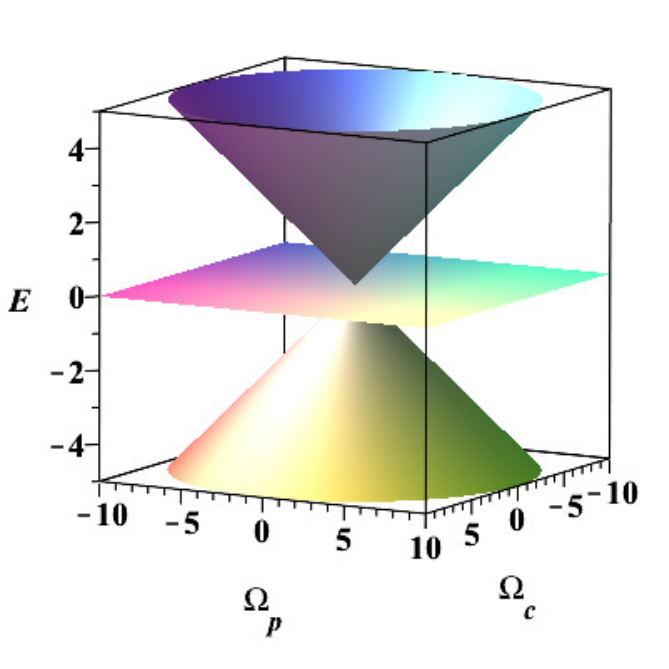
Suppose that that the two-foton excitation is resonant . In such conditions, the diagonalization of yields the following eigenenergies: and , where . We consider the complex Rabi frequencies and as control parameters living in , and set and , where . As one can see, the surfaces of the constant energies, , foliate by .
The eigenstate with the zero energy is called dark sate,
| (158) |
The remaining states with energies read
| (159) |
where is the bright state,
| (160) |
If one chooses the Rabi frequencies as
| (161) | |||||
| (162) |
then in the basis the dark and the bright states can be written as
where
| (169) |
Making use of these results for calculation of the induced gauge field we obtain
| (170) | ||||
| (171) |
Here we set and . One can gather all terms and recast Eqs. (170), (171) as,
| (172) |
where
| (173) |
Eq. (172) defines a natural or canonical connection on . The corresponding curvature , yielding a monopole field, reads
| (174) |
Remark. Geometric phases for two and three-level quantum systems governed by the Hamiltonian belonging to the Lie group or , respectively, are considered in details in Refs. KGMS; KAMN; BAY1.
Topological structures of adiabatic phase for multi-level quantum systems LZZX.
V.2.1 Laser beams with orbital angular momentum
Here we consider the laser beams with the orbital angular momentum and , so that and DGJ. This implies that the Rabi frequencies can be written as, and . Using these results in (170) and (171), we find
| (175) | ||||
| (176) |
where is the relative winding number of beams. From here we obtain
| (177) |
where
| (178) |
Below we will show that the charge belongs to the Lie algebra of the group , .
We look at the Rabi frequencies as the control parameters, taking them as , and . Thus the parameter space is three-dimensional manifold . We define a mapping as follows:
| (179) | |||||
| (180) |
where are the spherical coordinates in . The strength of the corresponding monopole field can be written as
| (181) |
An arbitrary monopole charge for monopole can be written as follows SHY:
| (182) |
where and are generators of Cartan subalgebra of ,
| (183) |
| (184) |
where are integers. Choosing and we obtain
| (185) |
The spin approach is recovered employing the unitary transformation
Under this transformation, the strength of the monopole field, (77), becomes
| (189) |
For general monopole, we obtain
| (190) |
where the first term defines the monopole spin, , and the second one, , describes its hypercharge.
To classify obtained solution one should look for stability group of and determine PJ. The generators of should commute with . There are generators of , that mix the two degenerated values of and generator given by Eq. (151). As was shown in PJ,
| (191) |
Next, using the identity and the fact that the fundamental group of is , one can obtain SHY
| (192) |
Thus, in general case the topological charge of the monopole is
| (193) |
where are integers. The quantization condition (151) takes the form:
| (194) |
Comparing this expression with (173), we find that .
Conclusion
In this paper, we studied the artificial magnetic monopoles associated with energy level crossing in quantum systems. In the simplest case of double degeneracy, the monopole is located at the degenerate point. Then, in the standard approach, one has two monopoles with similar structures of the magnetic field but with opposite charges. In the more complicated case of -level energy crossing there appear monopoles related to the corresponding eigenstates. Each monopole has its own charge, and the total charge of all monopoles equals zero B0; BD; Chj.
We show that in general case of -level energy crossing the quantum system can be successfully described by a single non-Abelian artificial ‘magnetic’ monopole with hidden symmetries and isospin degrees of freedom. In initial representation of the quantum system these hidden symmetries reveal themselves as a mixture of spin and other degrees of freedom.
In particular, for two-level system this monopole behaves as a quasi-particle with a spin one half. We demonstrated by different examples how the artificial monopole exposes itself. For a trapped -type system we found the monopole with the hidden symmetry . In this case, the monopole charge is fractional and represents the mixture of spin and Abelian charge degrees of freedom. These new features of artificial monopoles offer the possibility of the experimental test and can be useful in many physical applications.
Acknowledgements.
AIN acknowledges the support from the CONACyT. The work by G.P.B. was done at Los Alamos National Laboratory managed by Triad National Security, LLC, for the National Nuclear Security Administration of the U.S. Department of Energy under Contract No. 89233218CNA000001.References
- (1) E. Barouch, B.M. McCoy, Phys. Rev. A 3, 786 (1971)
- (2) R. Bhandari, Phys. Rev. Lett. 89, 268901 (2002)
- (3) Z. Fang et al, Science 302, 92 (2003)
- (4) C.M. Savage, J. Ruostekoski, Phys. Rev. A 68, 043604 (2003)
- (5) F.D.M. Haldane, Phys. Rev. Lett. 93, 206602 (2004)
- (6) J. Frenkel and S. H. Pereira, Phys. Rev. D 69, 127702 (2004)
- (7) P. Zhang, Y. Li, C.P. Sun, Eur. Phys. J. D 36, 229 (2005)
- (8) S. Morita, H. Nishimori, J. Math. Phys. 49, 125210 (2008)
- (9) V. Pietilä, M. Möttönen, Phys. Rev. Lett. 102, 080403 (2009)
- (10) J. Dalibard, F. Gerbier, G. Juzeliūnas, P. Öhberg, Rev. Mod. Phys. 83, 1523 (2011)
- (11) P. Račkauskas, V. Novičenko, H. Pu, G. Juzeliūnas, Phys. Rev. A 100, 063616 (2019)
- (12) V. Novičenko, G. Juzeliūnas, Phys. Rev. A 100, 012127 (2019)
- (13) G. Valentí-Rojas, N. Westerberg, P. Öhberg, Phys. Rev. Research 2, 033453 (2020)
- (14) S. Cusumano, A. De Pasquale, V. Giovannetti, Phys. Rev. Lett. 124, 190401 (2020)
- (15) M.W. Ray, E. Ruokokoski, M. Kandel, S. Mottonen, D.S. Hall, Nature 505, 657–660 (2014)
- (16) M.V. Berry, Proc. R. Soc. A 392, 45 (1984)
- (17) M.V. Berry, in Anomalies, Phases, Defects, ed. by U.M. Bregola, G. Marino, G. Morandi (Bibliopolis, Naples, 1990), p. 125
- (18) V.I. Arnold, Geometric Methods in the Theory of Ordinary Differential Equations (Springer, New York, 1983)
- (19) M.V. Berry, M. Wilkinson, Proc. Roy. Soc. A 392, 15 (1984)
- (20) M.V. Berry, M.R. Dennis, Proc. Roy. Soc. A 459, 1261 (2003)
- (21) Y. Aharonov, J. Anandan, Phys. Rev. Lett. 58(16), 1593 (1987)
- (22) F. Wilczek, A. Zee, Phys. Rev. Lett. 52, 2111 (1984)
- (23) C.A. Mead, Phys. Rev. Lett. 59, 161 (1987)
- (24) C.A. Mead, Rev. Mod. Phys. 64, 51 (1992)
- (25) A. Shapere, F. Wilczek (eds.), Geometric Phases in Physics (World Sci., Singapore, 1989)
- (26) P.A.M. Dirac, Proc. Roy. Soc. Lond. A 133, 60 (1931)
- (27) J. Schwinger, Phys. Rev. 144, 1087 (1966)
- (28) A.I. Nesterov, F. Aceves de la Cruz, Phys. Lett. A 302, 253 (2002)
- (29) A.I. Nesterov, Phys. Lett. A 328, 110 (2004)
- (30) T.T. Wu, C.N. Yang, Nucl. Phys. B 107, 365 (1976)
- (31) R. Jackiw, Phys. Rev. Lett. 54, 159 (1985)
- (32) R. Jackiw, Phys. Lett. B 154, 303 (1985)
- (33) G. Nadeau, Am. J. Phys. 28, 566 (1960)
- (34) I.R. I. Richard Lapidus, J.L. Pietenpol, Am. J. Phys. 28, 17 (1960)
- (35) D. Lynden-Bell, M. Nouri-Zonoz, Rev. Mod. Phys. 70, 427 (1998)
- (36) Y. Shnir, Magnetic Monopoles (Springer, New York, 2005)
- (37) H.A. Wilson, Phys. Rev. 75, 309 (1949)
- (38) A.S. Goldhaber, Phys. Rev. 140, B1407 (1965)
- (39) A.S. Goldhaber, Phys. Rev. Lett. 36, 1122 (1976)
- (40) M.N. Saha, Indian J. Phys. 10, 145 (1936)
- (41) M.N. Saha, Phys. Rev. 75, 1968 (1949)
- (42) F. Wilczek, Phys. Rev. Lett. 48, 1144 (1982)
- (43) F. Wilczek, Phys. Rev. Lett. 48, 1146 (1982)
- (44) R. Jackiw, C. Rebbi, Phys. Rev. Lett. 36, 1116 (1976)
- (45) P. Hasenfratz, G. ’t Hooft, Phys. Rev. Lett. 36, 1119 (1976)
- (46) J. Schwinger, Science 165, 757 (1969)
- (47) K.A. Milton, L.L. DeRaad, J. Math. Phys. 19 (1978)
- (48) K.A. Milton, Rep. Prog. Phys. 69, 1637 (2006)
- (49) D.N. Page, Phys. Rev. A 36, 3479 (1987)
- (50) B. Simon, Phys. Rev. Lett. 51, 2167 (1983)
- (51) D.C.A. Jamiolkowski, Geometric Phases in Classical and Quantum Mechanics (Birkhäuser, New York, 2004)
- (52) J. Anandan, L. Stodolsky, Phys. Rev. D 35, 2597 (1987)
- (53) M. Maamache, Y. Saadi, Phys. Rev. Lett. 101, 150407 (2008)
- (54) S. Massar, Phys. Rev. A 54, 4770 (1996)
- (55) N. Mukunda, R. Simon, Ann. Phys. 228, 205 (1993)
- (56) N. Mukunda, R. Simon, Ann. Phys. 228, 269 (1993)
- (57) J.C. Garrison, E.M. Wright, Phys. Lett. A 128, 177 (1988)
- (58) M.V. Berry, Ann. N. Y. Acad. Sci. 755, 303 (1995)
- (59) O.N. Kirillov, A.A. Mailybaev, A.P. Seyranian, J. Phys. A 38, 5531 (2005)
- (60) P. Hasenfratz, G. ’t Hooft, Phys. Rev. Lett. 36, 1119 (1976)
- (61) J. Moody, A. Shapere, F. Wilczek, Phys. Rev. Lett. 56, 893 (1986)
- (62) R. Jackiw, C. Rebbi, Phys. Rev. Lett. 36, 1116 (1976)
- (63) H.Z. Li, Phys. Rev. Lett. 58, 539 (1987)
- (64) H.Z. Li, Phys. Rev. D 35, 2615 (1987)
- (65) R. Jackiw, Phys. Rev. Lett. 56, 2779 (1986)
- (66) G.’t Hooft, Nuclear Physics B 79, 276 (1974)
- (67) A. Polyakov, Jetp Letters 20, 194 (1974)
- (68) J. Arafune, P.G.O. Freund, C.J. Goebel, J. Math. Phys. 16, 433 (1975)
- (69) V.I. Ritus, Zh. Eksp. Ter. Fiz. 51, 1544 (1966)
- (70) P. Brusheim, H.Q. Xu, Phys. Rev. B 79, 205323 (2009)
- (71) H. Sambe, Phys. Rev. A 7, 2203 (1973)
- (72) J. Hausinger, M. Grifoni, Phys. Rev. A 81, 022117 (2010)
- (73) D.J. Moore, J. Phys. A 23, L665 (1990)
- (74) D.J. Moore, J. Phys. A 23, 5523 (1990)
- (75) D.J. Moore, Phys. Rep. 210, 1 (1991)
- (76) M. Grifoni, P. Hanggi, Phys. Rep. 304, 229 (1998)
- (77) K. Aizu, J. Math. Phys. 4, 125210 (1963)
- (78) W.B. Brown, Proc. Cambridge. Phil. Soc. 54, 251 (1958)
- (79) J.H. Shirley, Phys. Rev. 138, B979 (1965)
- (80) E. Layton, Y. Huang, S.I. Chu, Phys. Rev. A 41, 42 (1990)
- (81) S. Coleman, Aspects of Symmetry: Selected Erice Lectures (Cambridge University Press, Cambridge, 1995)
- (82) S. Coleman, in Les Houches 1981, Proceedings, Gauge Theories in High Energy Physics, Part 1 (1983)
- (83) K. Osterloh, M. Baig, L. Santos, P. Zoller, M. Lewenstein, Phys. Rev. Lett. 95, 010403 (2005)
- (84) J. Ruseckas, G. Juzeliūnas, P. Öhberg, M. Fleischhauer, Phys. Rev. Lett. 95, 010404 (2005)
- (85) L.H. Lu, Y.Q. Li, Phys. Rev. A 76, 023410 (2007)
- (86) X.J. Liu, X. Liu, L.C. Kwek, C.H. Oh, Phys. Rev. Lett. 98, 026602 (2007)
- (87) G. Khanna, S. Mukhopadhyay, R. Simon, N. Mukunda, Annals of Physics 253, 55 (1997)
- (88) Arvind, K.S. Mallesh, N. Mukunda, Journal of Physics A: Mathematical and General 30(7), 2417 (1997)
- (89) Y. Ben-Aryeh, Optics and Spectroscopy 94(5), 724 (2003)
- (90) Z. Liu, X. Zhou, X. Liu, J. Chen, Journal of Physics A 40, 1661 (2007)
- (91) J. Preskill, Ann. Rev. of Nucl. and Part. Sci. 34, 461 (1984)