Topological Orders, Braiding Statistics, and Mixture of Two Types of Twisted $BF$ Theories in Five Dimensions

It is beneficial for us to review topological excitations and their braiding processes in $3$D and $4$D before we move into the $5$-dimensional spacetime. Anyon in the fractional quantum Hall effect (FQHE), a typical $3$D topological order, may be the most well-known example of topological excitations in $3$D. The self-statistics of anyons is captured by the phase difference after exchanging two anyons in the $2$D space. If viewed in $3$D, the world-lines of two anyons form a braid during the exchange. Geometrically, anyons are particle excitations, the only possible excitation in $3$D topological orders.²² 2 In $3$D topological orders, loop excitations are regarded equivalent to particle excitations. More concretely, because a loop excitation is impenetrable in $2$D space, it actually behaves like a particle excitation. Therefore, we do not consider loop excitations in $3$D topological orders. In $4$D topological orders, topological excitation spectrum is composed by particle excitations and loop excitations lantian3dto1; lantian3dto2. Braiding processes in $4$D topological orders can be divided into three classes zhang2021compatible: particle-loop braiding Witten1989; horowitz89; Horowitz1990; hansson2004superconductors; Baez2011; bti6, multi-loop (three or four) braiding wang_levin1; 2016arXiv161209298P, and particle-loop-loop braiding yp18prl. In particle-loop braiding, a particle excitation moves around a loop excitation such that its spatial trajectory and the loop excitation form a Hopf link. This Hopf link can also be identified from the intersection of the world-line of the particle and the world-sheet of the loop.³³ 3 For simplicity, when we mention particle, loop, or membrane, we refer to topological excitations in topological orders. In multi-loop braiding, three or four loops are linked in a special manner and their intersecting world-sheets indicate the topological invariant characterizing such braiding. In particle-loop-loop braiding, one particle moves around two unlinked loops such that its spatial trajectory and these two loops form Borromean rings yp18prl; RN874, or in general a Brunnian link.

In $5$D, besides particles and loops, there is a kind of exotic topological excitations, dubbed as membranes, which look like closed 2-dimensional surfaces⁴⁴ 4 We only consider membrane excitation that has a shape of a $2$-sphere in this paper. Membrane excitations with other shapes, e.g., $2$-torus, may have more fascinating properties.. The membrane excitations in $3$D space have not been considered because they are impenetrable. However, in $4$D space, the interior of a membrane excitation becomes accessible due to the extra dimension. Therefore, nontrivial braiding processes involving particles, loops and membranes are possible in $5$D.

In a braiding process of $5$D topological order, excitations move in $5$D spacetime in a particular manner, resulting in their $1$D world-line, $2$D world-sheet, and/or $3$D world-volume intersecting in a corresponding fashion. The $5$D TQFT can tell us about how these manifolds intersect in $5$D though which is not easy to imagine for us living in $3$D. To visualize braiding processes in $5$D topological order, we need to present them in lower dimensions. For this purpose, we can perform the following procedures. First, noticed that only the relative motion of excitations matters in a braiding process, we can assume one of the excitations to be static in $4$D space, then we project the world-lines/world-sheets/world-volumes from $5$D spacetime to $4$D space. For the static excitation, it is just fixed in $4$D space; for other excitations doing relative motion, their spatial trajectories are left in $4$D space after projection. An intuitive example is the anyon braiding in $3$D, shown in figure 1, in which the world-lines of anyons can be projected to spatial trajectories in $2$D plane.

Yet, the static excitation and spatial trajectories in $4$D space are still strange to observer in $3$D space. Our strategy is to furthermore project these spatial trajectories to slices of $4$D space, i.e., $3$D space. As an example, figure 2 shows the projection of spatial trajectory of particle-loop braiding from $3$D space to $2$D plane.

This example shows how an observer in $2$D space can understand braiding process in $4$D spacetime. In summary, by projecting the general world-lines in $5$D spacetime to spatial trajectories in $4$D space, then viewing them in $3$D slices, we can observe the braiding processes in $5$D topological order. This method will be explained by several pictures when discussing braiding and $5$D TQFT in the following main text.

As the effective theory of topological order, TQFT describes braiding processes by revealing how the world-lines (in general meaning) of excitations intersect in spacetime. A braiding process is nontrivial only if the world-lines of excitations form a link that is homotopic invariant. By constructing gauge-invariant observables, we know how to count the intersections of world-lines to obtain a result that is invariant under homotopic mapping of world-lines. In this and following sections, we use TQFT actions and gauge-invariant observables to study braiding processes in $5$D topological order.

The study of $BF$ term has a long history Horowitz1990. Discovered from quantum gravity and high energy physics, now $BF$ theories have been introduced into frontiers of condensed matter physics. In an $n$-dimensional spacetime manifold $M$, the $BF$ term is the wedge product of a $p$-form $\mathscr{B}$ and an $\left(n-p\right)$-form $\mathscr{F}=d\mathscr{A}$ where $\mathscr{A}$ is an $\left(n-p-1\right)$-form: $\mathscr{B}\wedge d\mathscr{A}$. $BF$ term in $3$D and $4$D reads $\tilde{A}dA$ and $BdA$ respectively, where $\tilde{A}$ and $A$ are $1$-form, $B$ is $2$-form. Theories with $BF$ terms have been applied to many different physical systems hansson2004superconductors; YeGu2015; bti2; bti6; bti1; Ye:2017aa; ye16a; PhysRevB.99.205120. It is easy to verify that $\tilde{A}dA$ ($BdA$) is the only $BF$ term in $3$D ($4$D). However, in $5$D, by taking $p=2$ or $p=3$, there are two types of $BF$ terms, i.e., $CdA$ and $\widetilde{B}dB$ which are respectively called type-I and type-II in this paper. Here, $C$ is a $3$-form, $\widetilde{B}$ and $B$ are two different $2$-form’s. These two types of $BF$ terms in $5$D are the cornerstone of this paper. With the action $S\sim\int_{M}\mathscr{B}d\mathscr{A}$, one can calculate the linking number of a $p$ and $\left(n-p-1\right)$-dimensional sub-manifolds Horowitz1990; 2016arXiv161209298P. In this section, we study the action with type-I and type-II $BF$ term in details, revealing the connection between braiding processes in $5$D topological orders and $BF$ terms.

We first look at the action with type-I $BF$ term:

$$S=\int\frac{N_{1}}{2\pi}C^{1}dA^{1},$$

(1)

which is invariant up to boundary term under gauge transformations

$$A^{1}\rightarrow A^{1}+d\chi^{1},\ C^{1}\rightarrow C^{1}+dT^{1},$$

(2)

where 0-form $\chi^{1}$ and 2-form $T^{1}$ are $\mathbb{U}\left(1\right)$ gauge parameters with $\oint d\chi^{1}\in 2\pi\mathbb{Z}$ and $\oint dT^{1}\in 2\pi\mathbb{Z}$. We consider the following gauge invariant observable (Wilson operator)

	$\displaystyle\mathcal{W}\left(\omega_{1},\gamma_{1}\right)=$	$\displaystyle\exp\left({\rm i}m_{1}\int_{\omega_{1}}C^{1}\right)\exp\left({\rm i}e_{1}\int_{\gamma_{1}}A^{1}\right)$
	$\displaystyle=$	$\displaystyle\exp\left[{\rm i}m_{1}\int C^{1}\wedge\delta^{\perp}\left(\omega_{1}\right)+{\rm i}e_{1}\int A^{1}\wedge\delta^{\perp}\left(\gamma_{1}\right)\right],$		(3)

where $\omega_{1}$ is a closed $3$D volume and $\gamma_{1}$ is a closed $1$D curve; charges $m_{1},e_{1}\in\mathbb{Z}$.⁵⁵ 5 Subscripts ($1,2,\cdots$, or general $i,j$) are used to distinguish manifolds that labeled by the same Greek letter. In this paper, $\gamma_{i}$ labels different $1$D closed curves; $\sigma_{i}$ and $\widetilde{\sigma}_{i}$ label different $2$D closed surfaces; $\omega_{i}$ stands for different $3$D closed volumes. $\Sigma_{i}$, $\Omega_{i}$, and $\Xi_{i}$ are the Seifert (hyper)surfaces: $\partial\Sigma_{i}=\gamma_{i}$, $\partial\Omega_{i}=\sigma_{i}$, and $\partial\Xi_{i}=\omega_{i}$. $\mu_{i}|_{X}$, $\nu_{i}|_{X}$, and $\lambda_{i}|_{X}$ respectively stand for general $1$D open curve, $2$D open surface, and $3$D open volume on manifold $X$. The expectation value is given by $\left\langle\mathcal{W}\left(\omega_{1},\gamma_{1}\right)\right\rangle=\frac{1}{\mathcal{Z}}\int\mathscr{D}A\mathscr{D}C\mathcal{W}\left(\omega_{1},\gamma_{1}\right)\exp\left({\rm i}S\right)$ where the partition function is defined as $\mathcal{Z}=\int\mathscr{D}C\mathscr{D}A\exp\left({\rm i}S\right)$. By integrating out $C^{1}$ we get $dA^{1}=-\frac{2\pi m_{1}}{N_{1}}\delta^{\perp}\left(\omega_{1}\right)$ which can be solved by $A^{1}=-\frac{2\pi m_{1}}{N_{1}}\delta^{\perp}\left(\Xi_{1}\right)$ with $\partial\Xi_{1}=\omega_{1}$, i.e., $\Xi_{1}$ is a Seifert hypersurface bounded by $\omega_{1}$. $\delta^{\perp}\left(\omega_{1}\right)$ is the $2$-form valued delta function distribution supported on $\omega_{1}$ and $\delta^{\perp}\left(\Xi_{1}\right)$ is similarly defined. Plugging the solution back to $\left\langle\mathcal{W}\left(\omega_{1},\gamma_{1}\right)\right\rangle$, we get

	$\displaystyle\left\langle\mathcal{W}\left(\omega_{1},\gamma_{1}\right)\right\rangle=$	$\displaystyle\exp\left[-\frac{{\rm i}2\pi e_{1}m_{1}}{N_{1}}\int\delta^{\perp}\left(\Xi_{1}\right)\wedge\delta^{\perp}\left(\gamma_{1}\right)\right]$
	$\displaystyle=$	$\displaystyle\exp\left[-\frac{{\rm i}2\pi e_{1}m_{1}}{N_{1}}\#\left(\Xi_{1}\cap\gamma_{1}\right)\right],$		(4)

i.e., $\left\langle\mathcal{W}\left(\omega_{1},\gamma_{1}\right)\right\rangle$ is determined by counting the intersection of $\Xi_{1}$ and $\gamma_{1}$. In $3$D, the linking number of two closed curves $\gamma_{i}$ and $\gamma_{j}$ is defined by the intersection number $\#\left(\Sigma_{i}\cap\gamma_{j}\right)$ where $\Sigma_{i}$ is a Seifert surface of $\gamma_{i}$. Analogous to this, $\#\left(\Xi_{1}\cap\gamma_{1}\right)$ defines the linking number of $\gamma_{1}$ and $\omega_{1}$ (whose Seifert hypersurface is $\Xi_{1}$) in $5$D. In Sec II.1, we mention that $5$D TQFT describes braiding process via intersection pattern of world-lines of excitations in $5$D. The action (1) and $\left\langle\mathcal{W}\left(\omega_{1},\gamma_{1}\right)\right\rangle$ describe the braiding process of a particle and a membrane once we interpret $\gamma_{1}$ ($\omega_{1}$) as the closed world-line (world-volume) of particle (membrane). Figure 3 illustrates this particle-membrane braiding by projecting it in different $3$D space.

Next we focus on the action that consists of a type-II $BF$ term:

$$S=\int\frac{N_{1}}{2\pi}\widetilde{B}^{1}dB^{1}$$

(5)

which is invariant up to boundary terms under

$$B^{1}\rightarrow B^{1}+dV^{1},\ \widetilde{B}^{1}\rightarrow\widetilde{B}^{1}+d\widetilde{V}^{1}.$$

(6)

Here, $1$-form $V^{1}$ and 1-form $\widetilde{V}^{1}$ are $\mathbb{U}\left(1\right)$ gauge parameters with $\oint dV^{1}\in 2\pi\mathbb{Z}$ and $\oint d\widetilde{V}^{1}\in 2\pi\mathbb{Z}$. We point out that $\widetilde{B}^{1}$ and $B^{1}$ are two independent $2$-form gauge field variables. The corresponding gauge-invariant observable is

$$\mathcal{W}\left(\widetilde{\sigma}_{1},\sigma_{1}\right)=\exp\left({\rm i}m_{1}\int_{\widetilde{\sigma}_{1}}\widetilde{B}^{1}\right)\exp\left({\rm i}e_{1}\int_{\sigma_{1}}B^{1}\right),$$

(7)

where $\widetilde{\sigma}_{1}$ and $\sigma_{1}$ are two closed $2$D surfaces; charges $m_{1},e_{1}\in\mathbb{Z}$. Similar to the calculation of $\left\langle\mathcal{W}\left(\omega_{1},\gamma_{1}\right)\right\rangle$ above, we get the solution $B^{1}=-\frac{2\pi m_{1}}{N_{1}}\delta^{\perp}\left(\widetilde{\Omega}_{1}\right)$ with $\partial\widetilde{\Omega}_{1}=\widetilde{\sigma}_{1}$, i.e., $\widetilde{\Omega}_{1}$ is a Seifert hypersurface bounded by $\widetilde{\sigma}_{1}$. Plugging this solution back, we obtain

	$\displaystyle\left\langle\mathcal{W}\left(\widetilde{\sigma}_{1},\sigma_{1}\right)\right\rangle=$	$\displaystyle\exp\left[-\frac{{\rm i}2\pi e_{1}m_{1}}{N_{1}}\int\delta^{\perp}\left(\widetilde{\Omega}_{1}\right)\wedge\delta^{\perp}\left(\sigma_{1}\right)\right]$
	$\displaystyle=$	$\displaystyle\exp\left[-\frac{{\rm i}2\pi e_{1}m_{1}}{N_{1}}\#\left(\widetilde{\Omega}_{1}\cap\sigma_{1}\right)\right],$		(8)

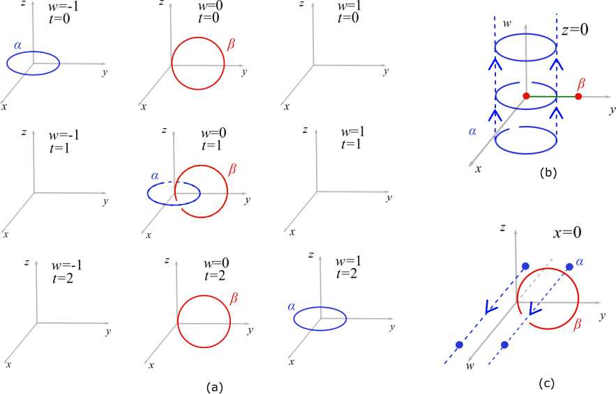
which indicates that $\left\langle\mathcal{W}\left(\widetilde{\sigma}_{1},\sigma_{1}\right)\right\rangle$ is determined by counting the intersection of $\widetilde{\Omega}_{1}$ and $\sigma_{1}$. Similarly, $\widetilde{\sigma}_{1}$ and $\sigma_{1}$ can be viewed as closed world-sheets of two loop excitations whose linking number is given by $\#\left(\widetilde{\Omega}_{1}\cap\sigma_{1}\right)$. Therefore, the type-II $BF$ term $\widetilde{B}^{1}dB^{1}$ describes to the braiding process of two loops and the braiding statistical phase can be extracted from $\left\langle\mathcal{W}\left(\widetilde{\sigma_{1}},\sigma_{1}\right)\right\rangle$. Figure 4 provides a diagrammatic representation of this loop-loop braiding by projecting the world-sheets to spatial trajectories of loops from $5$D to $4$D space.

So far we have investigated TQFT actions that consist of single $BF$ term. The coefficient $\frac{N_{1}}{2\pi}$ of the $BF$ term encodes the $\mathbb{Z}_{N_{1}}$ gauge group. If a $\prod_{i=1}^{n}\mathbb{Z}_{N_{i}}$ topological order is considered, i.e., the gauge group is $G=\prod_{i=1}^{n}\mathbb{Z}_{N_{i}}$, there are twisted terms allowed in TQFT actions besides $BF$ terms. As examples, we present some TQFT actions that consist of $BF$ terms and one twisted term in $4$D $\prod_{i=1}^{n}\mathbb{Z}_{N_{i}}$ topological orders Kapustin2014; YeGu2015; 2016arXiv161209298P; yp18prl; PhysRevB.99.235137; Tiwari:2016aa. With twisted term $AAdA$ or $AAAA$, TQFT actions $S=\int\sum_{i}\frac{N_{i}}{2\pi}B^{i}dA^{i}+qA^{i}A^{j}dA^{k}$ and $S=\int\sum_{i}\frac{N_{i}}{2\pi}B^{i}dA^{i}+qA^{i}A^{j}A^{k}A^{l}$ describe multi-loop braidings (three-loop and four-loop, respectively; $q$ is the proper coefficient). With twisted term $AAB$, the action $S=\int\sum_{i}\frac{N_{i}}{2\pi}B^{i}dA^{i}+qA^{i}A^{j}B^{k}$ describes the particle-loop-loop braiding. It is natural to expect that TQFT actions of $BF$ terms and twisted terms in $5$D are related to braiding processes of topological excitations. We divide the TQFT actions into $3$ classes according to the type of their $BF$ terms, namely type-I $BF$ theory, type-II $BF$ theory, and mixed $BF$ theory. In the remaining part of this section, we consider $BF$ theory with only one twisted term. Consistent combination of all twisted terms will be explored in section III.

We start with type-I $BF$ terms with a twisted term formed by $A$ and $C$, i.e., $AAC$, $AdAdA$, $AAAdA$, and $AAAAA$.

$AAC$ twisted topological term. By considering three $C^{i}dA^{i}$ terms, we can introduce the twisted term $A^{i}A^{j}C^{k}$. The corresponding TQFT action is

$$S=S_{BF}+S_{AAC}=\int\sum_{i=1}^{3}\frac{N_{i}}{2\pi}C^{i}dA^{i}+qA^{1}A^{2}C^{3},$$

(9)

where $q$ is a quantized and periodic coefficient, $q=\frac{pN_{1}N_{2}N_{3}}{\left(2\pi\right)^{2}N_{123}}$, $p\in\mathbb{Z}_{N_{123}}$, $N_{123}$ is the greatest common divisor of $N_{1}$, $N_{2}$ and $N_{3}$. The property of coefficient $q$ results from two requirements on the TQFT action: large gauge invariance and flux identification. In appendix A we derive the quantization and periodicity of $AAC$ and other twisted terms. It should be pointed out that the indices $i$, $j$, and $k$ in $A^{i}A^{j}C^{k}$ have to be mutually different. For example, the $A^{1}A^{2}C^{2}$ term is prohibited, because either $A^{2}$ or $C^{2}$ has to be the Lagrange multiplier, which means that they cannot simultaneously appear in the twisted term. A more rigorous explanation is that the an action with $A^{1}A^{2}C^{2}$ term would no more be gauge-invariant, which is similar to the $4$D case $S\sim\int\sum_{i=1}^{2}B^{i}dA^{i}+A^{1}A^{2}B^{2}$ studied in the Sec. IV A of ref. zhang2021compatible.

This action (9) is invariant under gauge transformations:

	$\displaystyle A^{1}\rightarrow A^{1}+d\chi^{1},\$	$\displaystyle C^{1}\rightarrow C^{1}+dT^{1}-\frac{2\pi q}{N_{1}}\left(\chi^{2}C^{3}-A^{2}T^{3}+\chi^{2}dT^{3}\right),$
	$\displaystyle A^{2}\rightarrow A^{2}+d\chi^{2},\$	$\displaystyle C^{2}\rightarrow C^{2}+dT^{2}+\frac{2\pi q}{N_{2}}\left(\chi^{1}C^{3}-A^{1}T^{3}+\chi^{1}dT^{3}\right),$
	$\displaystyle C^{3}\rightarrow C^{3}+dT^{3},\$	$\displaystyle A^{3}\rightarrow A^{3}+d\chi^{3}-\frac{2\pi q}{N_{3}}\left[\left(\chi^{1}A^{2}+\frac{1}{2}\chi^{1}d\chi^{2}\right)-\left(\chi^{2}A^{1}+\frac{1}{2}\chi^{2}d\chi^{1}\right)\right],$		(10)

where $\chi^{i}$ and $T^{i}$ are 0-form and 2-form gauge parameters, respectively. The gauge-invariant observable is

	$\displaystyle\mathcal{W}=$	$\displaystyle\exp\left\{{\rm i}\int_{\omega_{1}}e_{1}\left[C^{1}+\frac{1}{2}\frac{2\pi q}{N_{1}}\left(d^{-1}A^{2}C^{3}-d^{-1}C^{3}A^{2}\right)\right]\right.$
		$\displaystyle+{\rm i}\int_{\omega_{2}}e_{2}\left[C^{2}+\frac{1}{2}\frac{2\pi q}{N_{2}}\left(d^{-1}C^{3}A^{1}-d^{-1}A^{1}C^{3}\right)\right]$
		$\displaystyle+\left.{\rm i}\int_{\gamma_{3}}e_{3}\left[A^{3}+\frac{1}{2}\frac{2\pi q}{N_{3}}\left(d^{-1}A^{1}A^{2}-d^{-1}A^{2}A^{1}\right)\right]\right\}$		(11)

with $e_{1}$, $e_{2}$, and $e_{3}$ being integers. The derivation of gauge transformation (10) and verification of gauge-invariance of (11) is detailed in appendix B. The operation $d^{-1}$ is defined as $d^{-1}C^{3}|_{\omega_{i}}\equiv\int_{\lambda_{3}|_{\omega_{i}}}C^{3}$ where $\lambda_{3}|_{\omega_{i}}$ is an open $3$D volume on $\omega_{i}$ with $i=1,2$. As a $2$-form, $d^{-1}C^{3}$ is well-defined on $\omega_{i}$ if and only if $C^{3}$ is exact on $\omega_{i}$, i.e., $\int_{\omega_{i}}C^{3}=0$. The action of $d^{-1}$ on $A^{i}$ is defined as $d^{-1}A^{i}|_{\omega_{j}}\equiv\int_{\mu_{i}|_{\omega_{j}}}A^{i}$ and $d^{-1}A^{i}|_{\gamma_{3}}\equiv\int_{\mu_{i}|_{\gamma_{3}}}A^{i}$, where $\mu_{i}$ is an open curve on $\omega_{j}$ or $\gamma_{3}$. As a $0$-form, $d^{-1}A^{i}$ is well-defined on $\omega_{j}$ or $\gamma_{3}$ if and only if the integral of $A^{i}$ over any $1$-dimensional closed sub-manifolds of $\omega_{j}$ or $\gamma_{3}$ is zero. Since $A^{1}$, $A^{2}$, and $C^{3}$ are required to be exact on specific manifolds, it is straightforward that $dA^{1}$, $dA^{2}$, and $dC^{3}$ are zero on corresponding manifolds. This in fact guarantees the gauge invariance of (11). From a geometric perspective, the exactness condition implies restrictions that some sub-manifolds are not linked. In other words, the gauge invariance of observable is associated with the geometric interpretation of braiding process. The gauge fields and their fluxes are defined on specific sub-manifolds. For example, consider a gauge field $\mathscr{A}$ whose flux $d\mathscr{A}$ is defined on a closed $1$-manifold $\gamma_{1}$: $d\mathscr{A}=\delta^{\perp}\left(\gamma_{1}\right)$. Say, $\mathscr{A}$ is exact on another closed $1$-manifold $\gamma_{2}$, this means that $\int_{\Sigma}d\mathscr{A}=\int_{\gamma_{2}}\mathscr{A}=0$ with $\partial\Sigma=\gamma_{2}$. Since $\int_{\Sigma}d\mathscr{A}=\int\delta^{\perp}\left(\Sigma\right)\wedge\delta^{\perp}\left(\gamma_{1}\right)=\#\left(\Sigma\cap\gamma_{1}\right)$, the linking number of $\gamma_{1}$ and $\gamma_{2}$ is $0$ due to $\mathscr{A}$ is exact on $\gamma_{2}$. On the other hand, the gauge invariance of $\mathcal{W}$ ensures that $\left\langle\mathcal{W}\right\rangle$ is invariant under homotopic mapping of world-lines of excitations. However, sometimes $\left\langle\mathcal{W}\right\rangle$ does not clearly show how world-lines are linked . The exactness condition, required to meet gauge invariance, will give some hints since they reveal which sub-manifolds are not linked.

The expectation value is given by $\left\langle\mathcal{W}\right\rangle=\frac{1}{\mathcal{Z}}\int\mathscr{D}A\mathscr{D}C\mathcal{W}\exp\left({\rm i}S\right)$. Integrating out $C^{1}$, $C^{2}$, and $A^{3}$ implies $A^{1,2}=-\frac{2\pi e_{1,2}}{N_{1,2}}\delta^{\perp}\left(\Xi_{1,2}\right)$ and $C^{3}=-\frac{2\pi e_{3}}{N_{3}}\delta^{\perp}\left(\Sigma_{3}\right)$ with $\partial\Xi_{1,2}=\omega_{1,2}$ and $\partial\Sigma_{3}=\gamma_{3}$. Here, $\omega$ stands for $3$D closed volume, $\gamma$ stands for $1$D closed curve, etc, as explained in footnote 5. Putting these solutions back in $\left\langle\mathcal{W}\right\rangle$, we have

	$\displaystyle\int qA^{1}A^{2}C^{3}=$	$\displaystyle-\frac{\left(2\pi\right)^{3}qe_{1}e_{2}e_{3}}{N_{1}N_{2}N_{3}}\int\delta^{\perp}\left(\Xi_{1}\right)\wedge\delta^{\perp}\left(\Xi_{2}\right)\delta^{\perp}\left(\Sigma_{3}\right),$
	$\displaystyle=$	$\displaystyle-\frac{pN_{1}N_{2}N_{3}}{\left(2\pi\right)^{2}N_{123}}\frac{\left(2\pi\right)^{3}e_{1}e_{2}e_{3}}{N_{1}N_{2}N_{3}}\#\left(\Xi_{1}\cap\Xi_{2}\cap\Sigma_{3}\right)$
	$\displaystyle=$	$\displaystyle-\frac{2\pi pe_{1}e_{2}e_{3}}{N_{123}}\#\left(\Xi_{1}\cap\Xi_{2}\cap\Sigma_{3}\right);$		(12)

	$\displaystyle\int_{\omega_{1}}e_{1}\left[\frac{q}{2}\left(d^{-1}A^{2}C^{3}-d^{-1}C^{3}A^{2}\right)\right]=$	$\displaystyle\frac{\pi pe_{1}e_{2}e_{3}}{N_{123}}\left[\int\delta^{\perp}\left(\omega_{1}\right)\wedge\delta^{\perp}\left(\Sigma_{3}\right)\wedge d^{-1}\delta^{\perp}\left(\Xi_{2}\right)|_{\omega_{1}}\right.$
		$\displaystyle-\left.\int\delta^{\perp}\left(\omega_{1}\right)\wedge\delta^{\perp}\left(\Xi_{2}\right)\wedge d^{-1}\delta^{\perp}\left(\Sigma_{3}\right)|_{\omega_{1}}\right].$		(13)

By definition, $d^{-1}\delta^{\perp}\left(\Xi_{2}\right)|_{\omega_{1}}=\int_{\mu_{2}|_{\omega_{1}}}\delta^{\perp}\left(\Xi_{2}\right)=\int\delta^{\perp}\left(\mu_{2}|_{\omega_{1}}\right)\wedge\delta^{\perp}\left(\Xi_{2}\right)$, etc. Thus

	$\displaystyle\int_{\omega_{1}}e_{1}\left[\frac{q}{2}\left(d^{-1}A^{2}C^{3}-d^{-1}C^{3}A^{2}\right)\right]=$	$\displaystyle\frac{\pi pe_{1}e_{2}e_{3}}{N_{123}}\left[\int\delta^{\perp}\left(\omega_{1}\right)\wedge\delta^{\perp}\left(\Sigma_{3}\right)\wedge\int\delta^{\perp}\left(\mu_{2}|_{\omega_{1}}\right)\wedge\delta^{\perp}\left(\Xi_{2}\right)\right.$
		$\displaystyle-\left.\int\delta^{\perp}\left(\omega_{1}\right)\wedge\delta^{\perp}\left(\Xi_{2}\right)\wedge\int\delta^{\perp}\left(\lambda_{3}|_{\omega_{1}}\right)\wedge\delta^{\perp}\left(\Sigma_{3}\right)\right]$
	$\displaystyle=$	$\displaystyle\frac{\pi pe_{1}e_{2}e_{3}}{N_{123}}\left[\#\left(\omega_{1}\cap\Sigma_{3}\cap\mu_{2}|_{\omega_{1}}\cap\Xi_{2}\right)\right.$
		$\displaystyle-\left.\#\left(\omega_{1}\cap\Xi_{2}\cap\lambda_{3}|_{\omega_{1}}\cap\Sigma_{3}\right)\right].$		(14)

In a similar manner, we can calculate the remaining parts of $\left\langle\mathcal{W}\right\rangle$ and end up with

	$\displaystyle\left\langle\mathcal{W}\right\rangle=$	$\displaystyle\exp\left\{-\frac{{\rm i}2\pi pe_{1}e_{2}e_{3}}{N_{123}}\#\left(\Xi_{1}\cap\Xi_{2}\cap\Sigma_{3}\right)\right.$
		$\displaystyle+\frac{{\rm i}\pi pe_{1}e_{2}e_{3}}{N_{123}}\left[\#\left(\omega_{1}\cap\Sigma_{3}\cap\mu_{2}|_{\omega_{1}}\cap\Xi_{2}\right)-\#\left(\omega_{1}\cap\Xi_{2}\cap\lambda_{3}|_{\omega_{1}}\cap\Sigma_{3}\right)\right]$
		$\displaystyle+\frac{{\rm i}\pi pe_{1}e_{2}e_{3}}{N_{123}}\left[\#\left(\omega_{2}\cap\Xi_{1}\cap\lambda_{3}|_{\omega_{2}}\cap\Sigma_{3}\right)-\#\left(\omega_{2}\cap\Sigma_{3}\cap\mu_{1}|_{\omega_{2}}\cap\Xi_{1}\right)\right]$
		$\displaystyle+\left.\frac{{\rm i}\pi pe_{1}e_{2}e_{3}}{N_{123}}\left[\#\left(\gamma_{3}\cap\Xi_{2}\cap\mu_{1}|_{\gamma_{3}}\cap\Xi_{1}\right)-\#\left(\gamma_{3}\cap\Xi_{1}\cap\mu_{2}|_{\gamma_{3}}\cap\Xi_{2}\right)\right]\right\}.$		(15)

Geometrically, $\left\langle\mathcal{W}\right\rangle$ is determined by counting the intersections of several sub-manifolds in $5$D. According to their dimension, we can interpret their relations with excitations. The $1$D $\gamma_{i}$ can be understood as the closed world-line of particle. The $3$D $\omega_{i}$ can be regarded as the closed world-volume of membrane. $\Sigma_{i}$ and $\Xi_{i}$ are Seifert (hyper)surfaces: $\partial\Sigma_{i}=\gamma_{i}$ and $\partial\Xi_{i}=\omega_{i}$. We can see that all these sub-manifolds are related to one particle and two membranes. In this sense, we believe that the $AAC$ term along with its gauge-invariant observable (11) describe the braiding process of one particle and two membranes. Exploited with the exactness conditions, figure 5 illustrates this particle-membrane-membrane braiding in $3$D space.

In addition, the expectation value (15) is expressed as the sum of several terms: $\left\langle\mathcal{W}\right\rangle=\exp\left(-\frac{{\rm i}2\pi pe_{1}e_{2}e_{3}}{N_{123}}\mathfrak{L}\right)$ with

	$\displaystyle\mathfrak{L}=$	$\displaystyle\#\left(\Xi_{1}\cap\Xi_{2}\cap\Sigma_{3}\right)$
		$\displaystyle-\frac{1}{2}\left[\#\left(\omega_{1}\cap\Sigma_{3}\cap\mu_{2}|_{\omega_{1}}\cap\Xi_{2}\right)-\#\left(\omega_{1}\cap\Xi_{2}\cap\lambda_{3}|_{\omega_{1}}\cap\Sigma_{3}\right)\right]$
		$\displaystyle-\frac{1}{2}\left[\#\left(\omega_{2}\cap\Xi_{1}\cap\lambda_{3}|_{\omega_{2}}\cap\Sigma_{3}\right)-\#\left(\omega_{2}\cap\Sigma_{3}\cap\mu_{1}|_{\omega_{2}}\cap\Xi_{1}\right)\right]$
		$\displaystyle-\frac{1}{2}\left[\#\left(\gamma_{3}\cap\Xi_{2}\cap\mu_{1}|_{\gamma_{3}}\cap\Xi_{1}\right)-\#\left(\gamma_{3}\cap\Xi_{1}\cap\mu_{2}|_{\gamma_{3}}\cap\Xi_{2}\right)\right].$		(16)

$\#\left(\Xi_{1}\cap\Xi_{2}\cap\Sigma_{3}\right)$ counts the signed intersections of $\Xi_{1}$, $\Xi_{2}$ and $\Sigma_{3}$ and other terms have similar geometric meanings. Each term in $\mathfrak{L}$ (16) is not homotopic invariant because it depends on the choices of Seifert (hyper)surfaces. However, $\mathfrak{L}$ as the sum of these terms, is homotopic invariant due to the gauge invariance of $\left\langle\mathcal{W}\right\rangle$. We see that a mathematical invariant is obtained via physical gauge-invariant field theory. The formula of $\mathfrak{L}$ is similar to the equation (9) of ref. yp18prl which computes the Milnor’s triple linking number from a $4$D TQFT. In fact, the Milnor’s triple linking number of $3$ closed curves is also expressed as the sum of several homotopic-variant terms milnor1954link; mellor2003geometric. Analogously, eq. (16) can be regarded as the “triple linking number” of closed world-lines (in general meaning) of two membranes and one particle in $5$D. In the following main text, we will see more observables whose expectation values are expressed in a similar manner. It is interesting to reveal the mathematical structure behind them.

$AdAdA$ twisted topological term. Next, we consider the $AdAdA$ term, i.e., the Chern-Simons term in $5$D.⁶⁶ 6 When $BF$ term is not included, the theory is studied in ref. lapa17. For a gauge group $G=\prod_{i=1}^{n}\mathbb{Z}_{N_{i}}$, the type-I $BF$ theory with $AdAdA$ term has the form of

$$S=S_{BF}+S_{AdAdA}=\int\sum_{i=1}^{n}\frac{N_{i}}{2\pi}C^{i}dA^{i}+qA^{i}dA^{j}dA^{k}$$

(17)

with gauge transformations $A^{i}\rightarrow A^{i}+d\chi^{i}$ and $C^{i}\rightarrow C^{i}+dT^{i}$. The indices of $A^{i}dA^{j}dA^{k}$, same or different, take values from $\left\{1,2,\cdots,n\right\}$. The simplest type-I $BF$ theory with $AdAdA$ term is

$$S=\int\frac{N_{1}}{2\pi}C^{1}dA^{1}+qA^{1}dA^{1}dA^{1}$$

(18)

with $q=\frac{p}{\left(2\pi\right)^{2}}$, $p\in\mathbb{Z}_{N_{1}}$. This action (18) describes a $\mathbb{Z}_{N_{1}}$ $5$D topological order. The gauge-invariant observable for (18) is

$$\mathcal{W}=\exp\left({\rm i}e_{1}\int_{\omega_{1}}C^{1}\right)=\exp\left[{\rm i}e_{1}\int C^{1}\wedge\delta^{\perp}\left(\omega_{1}\right)\right]$$

(19)

with the expectation value

$$\left\langle\mathcal{W}\right\rangle=\exp\left[-\frac{{\rm i}2\pi pe_{1}e_{1}e_{1}}{N_{1}N_{1}N_{1}}\#\left(\Xi_{1}\cap\omega_{1}\cap\omega_{1}\right)\right].$$

(20)

If the gauge group is $G=\mathbb{Z}_{N_{1}}\times\mathbb{Z}_{N_{2}}$, the $AdAdA$ twisted term can also be $A^{1}dA^{2}dA^{1}$ or $A^{2}dA^{1}dA^{2}$. They are the only two linearly independent terms because $d\left(A^{1}A^{2}dA^{1}\right)=dA^{1}A^{2}dA^{1}-A^{1}dA^{2}dA^{1}$ and $d\left(A^{1}A^{2}dA^{2}\right)=dA^{1}A^{2}dA^{2}-A^{1}dA^{2}dA^{2}$. The corresponding type-I $BF$ theory and gauge-invariant observable is

	$\displaystyle S=$	$\displaystyle\int\sum_{i=1}^{2}\frac{N_{i}}{2\pi}C^{i}dA^{i}+qA^{1}dA^{2}dA^{1},$		(21)
	$\displaystyle\mathcal{W}=$	$\displaystyle\exp\left({\rm i}\sum_{i=1}^{2}e_{i}\int_{\omega_{i}}C^{i}\right)=\exp\left[{\rm i}\sum_{i=1}^{2}e_{i}\int C^{i}\wedge\delta^{\perp}\left(\omega_{i}\right)\right],$		(22)
	$\displaystyle\left\langle\mathcal{W}\right\rangle=$	$\displaystyle\exp\left[-\frac{{\rm i}2\pi pe_{1}e_{2}e_{1}}{N_{1}N_{2}N_{1}}\#\left(\Xi_{1}\cap\omega_{2}\cap\omega_{1}\right)\right];$		(23)

or

	$\displaystyle S^{\prime}=$	$\displaystyle\int\sum_{i=1}^{2}\frac{N_{i}}{2\pi}C^{i}dA^{i}+q^{\prime}A^{2}dA^{1}dA^{2},$		(24)
	$\displaystyle\mathcal{W}^{\prime}=$	$\displaystyle\exp\left({\rm i}\sum_{i=1}^{2}e_{i}\int_{\omega_{i}}C^{i}\right)=\exp\left[{\rm i}\sum_{i=1}^{2}e_{i}\int C^{i}\wedge\delta^{\perp}\left(\omega_{i}\right)\right],$		(25)
	$\displaystyle\left\langle\mathcal{W}^{\prime}\right\rangle=$	$\displaystyle\exp\left[-\frac{{\rm i}2\pi pe_{2}e_{1}e_{2}}{N_{2}N_{1}N_{2}}\#\left(\Xi_{2}\cap\omega_{1}\cap\omega_{2}\right)\right].$		(26)

The coefficients of twisted terms are $q=\frac{p}{\left(2\pi\right)^{2}}$, $p\in\mathbb{Z}_{N_{12}}$ and $q^{\prime}=\frac{p^{\prime}}{\left(2\pi\right)^{2}}$, $p^{\prime}\in\mathbb{Z}_{N_{12}}$; $\mathbb{Z}_{N_{12}}$ is the greatest common divisor of $N_{1}$ and $N_{2}$. The general case is that $G=\prod_{i=1}^{3}\mathbb{Z}_{N_{i}}$ in which the twisted term is $A^{1}dA^{2}dA^{3}$. In fact, $A^{1}dA^{2}dA^{3}$, $A^{2}dA^{3}dA^{1}$, and $A^{3}dA^{1}dA^{2}$ are identical up to a boundary term because $d\left(A^{1}A^{2}dA^{3}\right)=A^{2}dA^{3}dA^{1}-A^{1}dA^{2}dA^{3}$ and $d\left(A^{1}dA^{2}A^{3}\right)=A^{3}dA^{1}dA^{2}-A^{1}dA^{2}dA^{3}$. The type-I $BF$ theory with $A^{1}dA^{2}dA^{3}$ is

$$S=\int\sum_{i=1}^{3}\frac{N_{i}}{2\pi}C^{i}dA^{i}+qA^{1}dA^{2}dA^{3}$$

(27)

with $q=\frac{p}{\left(2\pi\right)^{2}}$, $p\in\mathbb{Z}_{N_{123}}$. For this type-I $BF$ theory (27), the gauge-invariant observable is

$$\mathcal{W}=\exp\left({\rm i}\sum_{i=1}^{3}e_{i}\int_{\omega_{i}}C^{i}\right)=\exp\left[{\rm i}\sum_{i=1}^{3}e_{i}\int C^{i}\wedge\delta^{\perp}\left(\omega_{i}\right)\right],$$

(28)

and its expectation value is

$$\left\langle\mathcal{W}\right\rangle=\exp\left[-\frac{{\rm i}2\pi pe_{1}e_{2}e_{3}}{N_{1}N_{2}N_{3}}\#\left(\Xi_{1}\cap\omega_{2}\cap\omega_{3}\right)\right].$$

(29)

We conclude that the $A^{i}dA^{j}dA^{k}$ twisted term describes the braiding process of three membranes, in which membranes move in $5$D leaving their intersecting world-volumes described by $\#\left(\Xi_{i}\cap\omega_{j}\cap\omega_{k}\right)$. For the action $S\sim\int\sum BdA+A^{i}dA^{j}dA^{k}$, the expectation value of gauge-invariant observable takes the form of $\left\langle\mathcal{W}\right\rangle\sim\exp\left[\#\left(\Xi_{i}\cap\omega_{j}\cap\omega_{k}\right)\right]$. All these three sub-manifolds are related with membranes: $\omega_{j}$ and $\omega_{k}$ can be regarded as the closed world-volumes of membrane $i$ and $j$; $\Xi_{i}$ is the Seifert hypersurface of $\omega_{i}$, the closed world-volume of membrane $i$. $\left(\Xi_{i}\cap\omega_{j}\cap\omega_{k}\right)$ can be seen as the intersection of three membranes’ world-volumes. Therefore, we believe that the $AdAdA$ term describes the braiding of three membrane whose phase shift is related to $\#\left(\Xi_{i}\cap\omega_{j}\cap\omega_{k}\right)$.

References

• (1) X.-G. Wen, Choreographed entanglement dances: Topological states of quantum matter, Science (2019) .
• (2) X.-G. Wen, A theory of 2+1d bosonic topological orders, Natl. Sci. Rev. (2015) [arXiv:1506.05768].
• (3) M. Levin and X.-G. Wen, Colloquium : Photons and electrons as emergent phenomena, Rev. Mod. Phys. 77 (2005) 871.
• (4) X.-G. Wen, Colloquium: Zoo of quantum-topological phases of matter, Rev. Mod. Phys. 89 (2017) 041004.
• (5) S. Hartnoll, S. Sachdev, T. Takayanagi, X. Chen, E. Silverstein and J. Sonner, Quantum connections, Nature Reviews Physics 3 (2021) 391.
• (6) A. Kitaev and J. Preskill, Topological entanglement entropy, Phys. Rev. Lett. 96 (2006) 110404.
• (7) M. Levin and X.-G. Wen, Detecting topological order in a ground state wave function, Phys. Rev. Lett. 96 (2006) 110405.
• (8) L. Kong and H. Zheng, A mathematical theory of gapless edges of 2d topological orders. part i, Journal of High Energy Physics 2020 (2020) 1.
• (9) L. Kong and H. Zheng, A mathematical theory of gapless edges of 2d topological orders. part ii, Nuclear Physics B 966 (2021) 115384.
• (10) C. Nayak, S.H. Simon, A. Stern, M. Freedman and S. Das Sarma, Non-abelian anyons and topological quantum computation, Rev. Mod. Phys. 80 (2008) 1083.
• (11) E. Witten, Quantum field theory and the jones polynomial, Commun. Math. Phys. 121 (1989) 351.
• (12) X.-G. Wen, Topological orders and edge excitations in fractional quantum hall states, Advances in Physics 44 (1995) 405 [https://doi.org/10.1080/00018739500101566].
• (13) X.-G. Wen, Classifying gauge anomalies through symmetry-protected trivial orders and classifying gravitational anomalies through topological orders, Phys. Rev. D 88 (2013) 045013.
• (14) L. Kong and X.-G. Wen, Braided fusion categories, gravitational anomalies, and the mathematical framework for topological orders in any dimensions, 2014.
• (15) M.A. Levin and X.-G. Wen, String-net condensation: A physical mechanism for topological phases, Phys. Rev. B 71 (2005) 045110.
• (16) Y.-S. Wu, General theory for quantum statistics in two dimensions, Phys. Rev. Lett. 52 (1984) 2103.
• (17) X. Chen, Z.-C. Gu and X.-G. Wen, Local unitary transformation, long-range quantum entanglement, wave function renormalization, and topological order, Phys. Rev. B 82 (2010) 155138.
• (18) A. Kitaev and C. Laumann, Topological phases and quantum computation, 0904.2771.
• (19) A. Kitaev, Anyons in an exactly solved model and beyond, Ann. Phys. 321 (2006) 2.
• (20) A.Y. Kitaev, Fault-tolerant quantum computation by anyons, Annals of Physics 303 (2003) 2 [quant-ph/9707021].
• (21) T. Lan, L. Kong and X.-G. Wen, Classification of (3+1)​D\mathbf{(}3+1\mathbf{)}\mathrm{D} bosonic topological orders: The case when pointlike excitations are all bosons, Phys. Rev. X 8 (2018) 021074.
• (22) T. Lan and X.-G. Wen, Classification of 3+1​D3+1\mathrm{D} bosonic topological orders (ii): The case when some pointlike excitations are fermions, Phys. Rev. X 9 (2019) 021005.
• (23) A.P.O. Chan, P. Ye and S. Ryu, Braiding with borromean rings in (3+13+1)-dimensional spacetime, Phys. Rev. Lett. 121 (2018) 061601.
• (24) X. Wen, H. He, A. Tiwari, Y. Zheng and P. Ye, Entanglement entropy for (3+1)-dimensional topological order with excitations, Phys. Rev. B 97 (2018) 085147.
• (25) C. Wang and M. Levin, Braiding statistics of loop excitations in three dimensions, Phys. Rev. Lett. 113 (2014) 080403.
• (26) P. Ye and Z.-C. Gu, Vortex-line condensation in three dimensions: A physical mechanism for bosonic topological insulators, Phys. Rev. X 5 (2015) 021029.
• (27) C.-M. Jian and X.-L. Qi, Layer construction of 3d topological states and string braiding statistics, Phys. Rev. X 4 (2014) 041043.
• (28) S. Jiang, A. Mesaros and Y. Ran, Generalized modular transformations in (3+1)​D(3+1)\mathrm{D} topologically ordered phases and triple linking invariant of loop braiding, Phys. Rev. X 4 (2014) 031048.
• (29) C. Wang, C.-H. Lin and M. Levin, Bulk-boundary correspondence for three-dimensional symmetry-protected topological phases, Phys. Rev. X 6 (2016) 021015.
• (30) Y. Wan, J.C. Wang and H. He, Twisted gauge theory model of topological phases in three dimensions, Phys. Rev. B 92 (2015) 045101.
• (31) P. Ye, T.L. Hughes, J. Maciejko and E. Fradkin, Composite particle theory of three-dimensional gapped fermionic phases: Fractional topological insulators and charge-loop excitation symmetry, Phys. Rev. B 94 (2016) 115104.
• (32) P. Ye and Z.-C. Gu, Topological quantum field theory of three-dimensional bosonic abelian-symmetry-protected topological phases, Phys. Rev. B 93 (2016) 205157.
• (33) A. Kapustin and R. Thorngren, Anomalies of discrete symmetries in various dimensions and group cohomology, ArXiv e-prints (2014) [1404.3230].
• (34) P. Ye and X.-G. Wen, Constructing symmetric topological phases of bosons in three dimensions via fermionic projective construction and dyon condensation, Phys. Rev. B 89 (2014) 045127.
• (35) S.-Q. Ning, Z.-X. Liu and P. Ye, Symmetry enrichment in three-dimensional topological phases, Phys. Rev. B 94 (2016) 245120.
• (36) S.-Q. Ning, Z.-X. Liu and P. Ye, Topological gauge theory, symmetry fractionalization, and classification of symmetry-enriched topological phases in three dimensions, arXiv e-prints (2018) [1801.01638].
• (37) P. Ye, Three-dimensional anomalous twisted gauge theories with global symmetry: Implications for quantum spin liquids, Phys. Rev. B 97 (2018) 125127.
• (38) J.C. Wang and X.-G. Wen, Non-abelian string and particle braiding in topological order: Modular SL⁡(3,ℤ)\mathrm{SL}(3,\mathbb{Z}) representation and (3+1)(3+1)-dimensional twisted gauge theory, Phys. Rev. B 91 (2015) 035134.
• (39) J.C. Wang, Z.-C. Gu and X.-G. Wen, Field-theory representation of gauge-gravity symmetry-protected topological invariants, group cohomology, and beyond, Phys. Rev. Lett. 114 (2015) 031601.
• (40) X. Chen, A. Tiwari and S. Ryu, Bulk-boundary correspondence in (3+1)-dimensional topological phases, Phys. Rev. B 94 (2016) 045113.
• (41) J. Wang, X.-G. Wen and S.-T. Yau, Quantum Statistics and Spacetime Surgery, ArXiv e-prints (2016) [1602.05951].
• (42) P. Putrov, J. Wang and S.-T. Yau, Braiding statistics and link invariants of bosonic/fermionic topological quantum matter in 2+1 and 3+1 dimensions, Annals of Physics 384 (2017) 254 .
• (43) P. Ye, M. Cheng and E. Fradkin, Fractional ss-duality, classification of fractional topological insulators, and surface topological order, Phys. Rev. B 96 (2017) 085125.
• (44) A. Tiwari, X. Chen and S. Ryu, Wilson operator algebras and ground states of coupled 𝐵𝐹\mathit{BF} theories, Phys. Rev. B 95 (2017) 245124.
• (45) K. Walker and Z. Wang, (3+1)-TQFTs and topological insulators, Frontiers of Physics 7 (2012) 150 [1104.2632].
• (46) Z.-F. Zhang and P. Ye, Compatible braidings with hopf links, multiloop, and borromean rings in (3+1)(3+1)-dimensional spacetime, Phys. Rev. Research 3 (2021) 023132.
• (47) M.-Y. Li and P. Ye, Fracton physics of spatially extended excitations, Phys. Rev. B 101 (2020) 245134.
• (48) M.-Y. Li and P. Ye, Fracton physics of spatially extended excitations. II. Polynomial ground state degeneracy of exactly solvable models, arXiv e-prints (2021) arXiv:2104.05735 [2104.05735].
• (49) S. Pai and M. Pretko, Fractonic line excitations: An inroad from three-dimensional elasticity theory, Phys. Rev. B 97 (2018) 235102.
• (50) T.H. Hansson, V. Oganesyan and S.L. Sondhi, Superconductors are topologically ordered, Annals of Physics 313 (2004) 497.
• (51) Y. Aharonov and D. Bohm, Significance of electromagnetic potentials in the quantum theory, Phys. Rev. 115 (1959) 485.
• (52) J. Preskill and L.M. Krauss, Local discrete symmetry and quantum-mechanical hair, Nuclear Physics B 341 (1990) 50 .
• (53) M.G. Alford and F. Wilczek, Aharonov-bohm interaction of cosmic strings with matter, Phys. Rev. Lett. 62 (1989) 1071.
• (54) L.M. Krauss and F. Wilczek, Discrete gauge symmetry in continuum theories, Phys. Rev. Lett. 62 (1989) 1221.
• (55) M.G. Alford, K.-M. Lee, J. March-Russell and J. Preskill, Quantum field theory of non-abelian strings and vortices, Nuclear Physics B 384 (1992) 251 .
• (56) G.T. Horowitz and M. Srednicki, A quantum field theoretic description of linking numbers and their generalization, Communications in Mathematical Physics 130 (1990) 83.
• (57) G.T. Horowitz, Exactly soluble diffeomorphism invariant theories, Commun. Math. Phys. 125 (1989) 417.
• (58) J.C. Baez and J. Huerta, An invitation to higher gauge theory, General Relativity and Gravitation 43 (2011) 2335.
• (59) P. Ye and J. Wang, Symmetry-protected topological phases with charge and spin symmetries: Response theory and dynamical gauge theory in two and three dimensions, Phys. Rev. B 88 (2013) 235109.
• (60) P. Cromwell, E. Beltrami and M. Rampichini, The mathematical tourist, The Mathematical Intelligencer 20 (1998) 53.
• (61) A. Vishwanath and T. Senthil, Physics of three-dimensional bosonic topological insulators: Surface-deconfined criticality and quantized magnetoelectric effect, Phys. Rev. X 3 (2013) 011016.
• (62) B. Han, H. Wang and P. Ye, Generalized wen-zee terms, Phys. Rev. B 99 (2019) 205120.
• (63) A. Kapustin and N. Seiberg, Coupling a qft to a tqft and duality, Journal of High Energy Physics 2014 (2014) 1.
• (64) Q.-R. Wang, M. Cheng, C. Wang and Z.-C. Gu, Topological quantum field theory for abelian topological phases and loop braiding statistics in (3+1)(3+1)-dimensions, Phys. Rev. B 99 (2019) 235137.
• (65) J. Milnor, Link groups, Ann. Math. 59 (1954) 177.
• (66) B. Mellor and P. Melvin, A geometric interpretation of milnor’s triple linking numbers, Algebr. Geom. Topol. 3 (2003) 557.
• (67) M.F. Lapa, C.-M. Jian, P. Ye and T.L. Hughes, Topological electromagnetic responses of bosonic quantum hall, topological insulator, and chiral semimetal phases in all dimensions, Phys. Rev. B 95 (2017) 035149.
• (68) D. Gaiotto, A. Kapustin, N. Seiberg and B. Willett, Generalized global symmetries, J. High Energy Phys. 2015 (2015) 1.
• (69) C.W. von Keyserlingk and F.J. Burnell, Walker-wang models and axion electrodynamics, Phys. Rev. B 91 (2015) 045134.
• (70) X. Chen, A. Dua, P.-S. Hsin, C.-M. Jian, W. Shirley and C. Xu, Loops in 4+1d Topological Phases, arXiv e-prints (2021) arXiv:2112.02137 [2112.02137].