The Intrinsic Scatter of Galaxy Scaling RelationsJournal: The Astrophysical Journalastropy (Price-Whelan et al. 2018), photutils (Bradley et al. 2020), numpy (Harris et al. 2020), scipy (Jones et al. 2001)
Abstract
We present a compendium of disk galaxy scaling relations and a detailed characterization of their intrinsic scatter. Observed scaling relations are typically characterized by their slope, intercept, and scatter; however, these parameters are a mixture of observational errors and astrophysical processes. We introduce a novel Bayesian framework for computing the intrinsic scatter of scaling relations that accounts for nonlinear error propagation and covariant uncertainties. Bayesian intrinsic scatters are percent more accurate than those obtained with a first-order classical method, which systematically underestimates the true intrinsic scatter. Structural galaxy scaling relations based on velocity (), size (), luminosity (), colour (), central stellar surface density (), stellar mass (), dynamical mass (), stellar angular momentum (), and dynamical angular momentum (), are examined to demonstrate the power and importance of the Bayesian formalism. Our analysis is based on a diverse selection of over 1000 late-type galaxies from the Photometry and Rotation Curve Observations from Extragalactic Surveys compilation with deep optical photometry and extended rotation curves. We determine the tightest relation for each parameter by intrinsic orthogonal scatter, finding , , and to be especially tight. The scatter of the , , and relations is mostly intrinsic, making them ideal for galaxy formation and evolutionary studies. Our code to compute the Bayesian intrinsic scatter of any scaling relation is also presented. We quantify the correlated nature of many uncertainties in galaxy scaling relations and scrutinize the uncertain nature of disk inclination corrections and their effect on scatter estimates.
Keywords:
galaxies: general – galaxies: spiral – galaxies: kinematics and dynamics – galaxies: statistics – methods: statistical – techniques: miscellaneousI Introduction
Scaling relations are a critical component of any characterization and understanding of galaxy formation and evolutionary scenarios. For instance, a necessary benchmark for the success and fine-tuning of hydrodynamics or semi-analytic models of galaxies is the degree to which they reproduce the slope and scatter of known scaling relations for observed galaxies (Steinmetz & Navarro 1999; Brook et al. 2012b; Scannapieco et al. 2012; Knebe et al. 2018; Lagos et al. 2018). In addition, one can describe the evolution of galaxies with time (redshift) in terms of scaling relations (Mo et al. 1998; Hopkins et al. 2009; Peng et al. 2010; van der Wel et al. 2014; Mowla et al. 2019). Scaling relations of observed galaxies and their residuals are also valuable for estimating galaxy distances (Tully & Fisher 1977; Jacoby et al. 1992; Willick 1999; Sakai et al. 2000; Kourkchi et al. 2020) and fine-tuning structural parameter corrections (Tully & Fouqué 1985; Giovanelli et al. 1994; Willick et al. 1997; Courteau et al. 2007; Giovanelli 2013). They can also drive the discovery of new physical relationships (Bender et al. 1993; Woo et al. 2008; Beifiori et al. 2012; Ellison et al. 2020).
Galaxy scaling relations are typically linear in log scale and are therefore characterized by three quantities: slope, intercept, and scatter. Cold Dark Matter (CDM) galaxy formation models that match both the abundance and size distribution of galaxies can reproduce some galaxy scaling relations such as velocity-luminosity, also known as the Tully-Fisher relation (Tully & Fisher 1977, TFR;), with reasonable accuracy (Dutton et al. 2011; Brook et al. 2012b; Ferrero et al. 2017). Simultaneously matching multiple scaling relations is, however, a challenging task (Dutton et al. 2011; Trujillo-Gomez et al. 2011). Small changes to a numerical model can indeed result in significant changes to slope, intercept, and/or scatter for one or more scaling relations simultaneously (Dutton et al. 2010; Brook et al. 2012a; Kim et al. 2014; Schaller et al. 2015).
Scaling relation slopes and scatters reported in the literature can vary greatly as a result of the many different selection functions, systematic errors from heterogeneous reduction and analysis methods, observational errors, bandpass sensitivities, and other effects (see Section V). Short of being able to correct for all biases and systematic differences, attempts to compare empirical scaling relations with theoretical models of galaxy structure require at least that most (tractable) observational errors be removed (Strauss & Willick 1995; Pizagno et al. 2005; Pizagno et al. 2007; Saintonge & Spekkens 2011; Lelli et al. 2017). In this work, we present a detailed framework for the simultaneous derivation of the intrinsic scatter estimates for numerous galaxy scaling relations.
The intrinsic slope, intercept and total scatter of a scaling relation can be found to arbitrary precision (limit of random error goes to zero) by fitting a model to a large unbiased galaxy sample. However, the intrinsic scatter must also be inferred by modeling uncertainties. Due to the complex and heteroscedastic nature of observational uncertainties in astronomy, accounting for their impact in empirical studies can be challenging (Isobe et al. 1990; Andreon & Hurn 2013). Two broad paths are typically explored to connect galaxy observations and models. One path consists of generating mock observations of a model by introducing uncertainties tuned to a specific observational campaign (Jonsson et al. 2010; Snyder et al. 2015; Torrey et al. 2015; Bottrell et al. 2017; Yung et al. 2019). This technique has the advantage of being flexible; once the mock observations are complete, one can apply standard analysis pipelines and produce any desired quantity for a large sample size. The results are however nontransferable between different models and observations, and so must be redone for each model-observation pair. The second path accounts directly for uncertainties and effectively subtracts their effects from an analysis of observational data in order to arrive at intrinsic quantities. This second method is in principle preferable since physically meaningful results are directly extracted and can instantly be compared with any model. The main drawback of this approach is the complexity in accounting for sample completeness, bias, and uncertainty in the data.
The TFR is a case where the intrinsic scatter has been inferred from observations (Bernstein et al. 1994; Gnedin et al. 2007; Pizagno et al. 2007; Reyes et al. 2011; Saintonge & Spekkens 2011), and likewise for the radial acceleration relation (McGaugh 2004; McGaugh et al. 2016; Lelli et al. 2017) where intrinsic scatters can differentiate physical models (McGaugh et al. 2016; Rong et al. 2018; Stone & Courteau 2019). However, intrinsic scatter estimates in some of these examples are determined to first order by subtracting the average uncertainty in quadrature. This “classical” analysis (detailed in Section II.2) has notable drawbacks, including the absence of correlated uncertainties and an assumption of linearity in all transformations, not to mention the possibility of returning nonphysical negative scatters. In contrast, some weak lensing scaling relations are now benefiting from Bayesian estimates of intrinsic scatter that more robustly account for sources of error (Sereno & Ettori 2015).
In this work, we present a Bayesian framework for analyzing intrinsic scatter and apply it to a suite of well-known structural and dynamical galaxy scaling relations. This framework is easily implemented numerically and provides robust measures of intrinsic scatter, even when confronted with certain biases that the classical analysis cannot take into consideration (Appendix B).
This paper is organized as follows. We begin by modeling the scatter of a general scaling relation in Section II and explicitly define the classical and Bayesian procedures for evaluating intrinsic scatters. Section III then describes the Photometry and Rotation Curve Observations from Extragalactic Surveys (PROBES) compilation that is used in our analysis; it represents the largest collection of deep long slit spectroscopic rotation curves coupled with deep multiband photometry to date. Section IV presents the fit results and intrinsic scatter measurements following the outlined analysis techniques. Section V performs a detailed literature comparison with our results and many others, including a comparison of intrinsic scatters where available. We expound in Section VI on robust measures of intrinsic scatter as a powerful metric for validating and improving galaxy evolutionary models. For more information on the numerical technique, see Appendix B where we present the numerical method to compute Bayesian intrinsic scatters and tests of the technique’s stability. Appendix C provides a minimalist python implementation of the Bayesian intrinsic scatter code for ease of use by other authors. In Section III.4 we explore the uncertain nature of inclination corrections and the importance of a multi-scaling relation analysis to determine their true form.
II Intrinsic Scatter Model
We have noted that any (linear) scaling relation can be represented by a slope, intercept, and scatter. This section pertains specifically to the characterization of a scaling relation’s intrinsic scatter. Modeling the scatter of a scaling relation involves clearly defining the source of each perturbation on a data point and tracking their effect on the position of this point in a given mathematical transformation. We express the mathematical model used to define intrinsic scatter and its relation to observational uncertainties. In a classical framework, the intrinsic scatter is calculated by averaging the observational uncertainties to first order and subtracting them in quadrature from the total observed scatter. In a Bayesian framework, a posterior is constructed for the intrinsic scatter by marginalizing over all observational uncertainties. Both frameworks are reviewed below.
II.1 Scatter Model for Scaling Relations
We first assume a vector of variables that describes the measurements taken of an object (e.g. a galaxy). A scaling relation is constructed using the functions and for each axis. Some values in may not be used in the or functions and some may be used by both (likely leading to covariance); simply represents all necessary inputs to compute the relation. The scaling relation is a function such that for a “perfect” relation. Nature does not produce perfect (scatter-free) relations though; instead, every object (galaxy) will suffer a perturbation from the relation drawn from an intrinsic scatter distribution. Since the exact nature of the intrinsic scatter cannot be recovered exactly, its form is assumed to be a normal distribution, which scatters about the -axis. There is some loss of generality in the assumption of normal distribution; however there is no compelling reason to suspect otherwise. Thus our scaling relation can be written where is the perturbation drawn from where is a normal distribution probability density function (pdf) and is the intrinsic scatter.
The quantities cannot be measured perfectly, and we measure instead where is some perturbation drawn from where are the uncertainties for each variable. For each measured quantity, we have access to the measurement () and the uncertainty (); the specific intermediate is unknown though its distribution is known.
The residuals from a scaling relation can then be decomposed into their measurement uncertainty and intrinsic scatter components. Forward residuals are represented as which after decomposition look like . Thus the residual can be measured, but and are unknown. Recovering , which generates the distribution, can be achieved in various ways as we address below. Section II.2 presents the classical first-order method and Section II.3 presents our more careful Bayesian technique.
II.2 Classical Intrinsic Scatter
In the classical framework, the observed scatter () and uncertainty scatter () of a scaling relation are computed to first order and subtracted in quadrature to produce the intrinsic scatter. Assuming a normal distribution, the observed scatter is computed with a standard deviation of the forward residuals; estimating the scatter due to uncertainty is more complex. For an individual data point, the uncertainty scatter is computed as:
| (1) |
where is the -axis scatter, is a variable used in computing the relation, is the derivative of the relation with respect to variable , and is the uncertainty on variable . In the specific context of galaxy scaling relations, data are highly heteroscedastic, and a procedure for averaging the uncertainties is required. The average of the variances (not the standard deviation ) gives an unbiased estimator of the scatter due to observational uncertainties:
| (2) |
where is the total number of observations. The intrinsic scatter is then computed as . Note that while this formula may produce negative intrinsic scatters, these values must be reported despite the unrealistic value for the estimator to be unbiased on average. The value of interest is , not , and so a square root must be taken. In the event that is negative, we report a negative ; the estimator for is therefore . A confidence interval for can be determined using bootstrap sampling (Efron 1992).
II.3 Bayesian Intrinsic Scatter
The Bayesian framework involves marginalizing over all observational uncertainties, leaving a pdf for possible intrinsic scatter values. If were known, we could write for each galaxy and construct a pdf for directly. Since is unknown (only the distribution from which it is drawn), we construct:
| (3) |
which corresponds to the probability of obtaining the residual () given a proposed intrinsic scatter () and perturbation () combination. A notable aspect of the algorithm presented in Equation 3 is the generality of the function , such that our Bayesian intrinsic scatters may be computed for any scaling relation for which residuals are measured. The marginalization over the pdf () of possible values yields a pdf of . Bayes Theorem is then used to convert the result into a pdf for intrinsic scatter:
| (4) | ||||
where is the prior for the intrinsic scatter (we use a flat prior from zero to the total scaling relation scatter) and is the normalization. The product of all posteriors is used to combine the results for many objects (galaxies). While simple, this procedure cannot be computed analytically; instead, numerical techniques must be used to perform the integral in Equation 4. Section II.4 presents such a procedure for computing the integral. Tests demonstrating the robustness of the Bayesian method relative to the classical method with a toy model are also presented in Appendix B. In our idealized toy model, the estimates of the Bayesian intrinsic scatter have at minimum a relative accuracy improvement over classical estimates; however many factors influence the true error for a real scaling relation. A code to compute a Bayesian intrinsic scatter is also presented in Appendix C.
II.4 Numerical Bayesian Intrinsic Scatters
The procedure for marginalizing over observational uncertainties to get the intrinsic scatter of a scaling relation described in Section II.3 cannot be completed analytically; however, numerical techniques can achieve arbitrary precision. The integration in Equation 4 can numerically be performed with relative ease, though with a slightly modified procedure. Depicted in Figure 1 are the critical steps of the numerical procedure as performed with a toy model.
The toy model data in Figure 1-a are constructed as follows. Five-hundred mock “galaxies” are sampled from a two-dimensional Gaussian distribution (only 50 shown for clarity) forming the true distribution of the galaxies () with intrinsic scatter as the forward residual standard deviation. Each data point is assigned a unique observational uncertainty () in the -axis and -axis separately by drawing an uncertainty from a uniform distribution over the range , thus making the data heteroscedastic. The data points are then perturbed by sampling normal distributions with variance determined by their assigned observational uncertainty; this simulates the perturbations giving . The Bayesian algorithm knows only the final position of the data points () and the assigned observational uncertainty for each data point (). The data are fit with a BCES bisector algorithm (see Section IV.1) and all residuals are computed relative to this.
In Figure 1-b the observational uncertainties () are numerically integrated over by sampling their distribution 500 times (only 100 shown for clarity). In Figure 1-c the residuals of the samples form a pdf for the perturbation given the observed data point and observational uncertainties. Figure 1-d shows the likelihood for as a function of possible values. This is essentially an inverted gaussian distribution, the probability density is plotted by varying for a fixed x (not the other way around) where x is a single residual value after sampling in Figure 1-b. In Figure 1-e, the “integral” is performed by summing each likelihood at a given value, and Bayes theorem is used to turn this into a pdf for . Only two examples are shown for clarity, one that favours low values and one that favours large values. Finally, in Figure 1-f, the product of all posteriors is taken to give the posterior for the full dataset in Figure 1-a.
III PROBES Sample
We have described a new and powerful method for computing intrinsic scatters for arbitrary scaling relations. To demonstrate the general usefulness of this algorithm, we will apply it to a compendium of galaxy scaling relations. We begin by describing the data used in our analysis.
The PROBES compilation combines several rotation curve surveys and homogeneous photometry from the Dark Energy Spectroscopic Instrument Legacy Imaging Survey (Dey et al. 2019, DESI-LIS;). Here we describe the parameter extraction techniques used in this analysis as well as the choices for corrections, uncertainty propagation, and data quality cuts.
III.1 Light Profile Extraction Using AutoProf
Photometry for our analysis comes from the DESI-LIS, which provides images in the , , and bands for a large ( deg2) section of the sky (Dey et al. 2019). The intersection of DESI-LIS and PROBES (Section III.2.1) totals 1396 galaxies to be used for our analysis, with some removed due to selection cuts described in Section III.6. Images are processed using our surface photometry package, AutoProf, which is briefly described below.
AutoProf is our Python-based galaxy image isophotal solution pipeline, with functions for center finding, background subtraction, star masking, isophote fitting, and surface brightness profile extraction. Center finding uses centering methods from the photutils Python package (Bradley et al. 2020) or with a user-defined center (in pixel coordinates). Background subtraction and star masking are also completed using standard tools from the photutils package. Star masking is generally turned off by default, but wrappers are included for IRAF star finding (Tody 1986) and the DAO star finder (Stetson 1987). The isophote optimization algorithm minimizes the amplitude of low-order fast Fourier transform coefficients (Cooley & Tukey 1965) for flux values evaluated around an isophote, plus a regularization term (Shai Shalev-Shwartz 2014). The regularization term penalizes large differences in ellipticity and position angle between adjacent isophotes using the norm (the sum of squared differences; also see Shai Shalev-Shwartz 2014). This effectively smooths out the isophotal solution while not setting any explicit boundaries on the difference between adjacent isophotes. In some cases, typically for non-axisymmetric features such as bars or strong spiral arms, it is desirable to allow for large variations in ellipticity and/or position angle. Multiple isophotes are fit simultaneously; these are selected with geometrically growing radii out to a signal-to-noise ratio (S/N) of (typically ), beyond which the ellipticity and position angle are taken as constant. To sample a surface brightness profile, the isophotal solution ellipticity and position angle are linearly interpolated allowing for any desired sampling of the image. Surface brightnesses are taken as the median flux from many sample points around an isophote, and so most foreground stars need not be masked from an image as they will be ignored by the median. A curve of growth is computed as the integral of the surface brightness profile; the summed flux of all pixels within each isophote is reported as well. The fluxes are converted to the AB magnitude system11 1 See Dey et al. 2019 and https://www.legacysurvey.org/dr8/description/ for specifics of the DESI-LIS photometry.
Isophotal solutions are visually inspected to identify possible failures such as those involving non-axisymmetric features. Most PROBES galaxies already have archival photometry available, though for a limited range of photometric bands. These (heterogeneous) light profiles were used to validate the accuracy of the automated DESI-LIS photometry. Galaxies deemed to have failed the visual isophote inspection or deviate in some pathological way from the older PROBES photometry were discarded. The surface brightness profiles are evaluated out to a typical photometric depth in the band of roughly before reaching a cutoff uncertainty of . AutoProf will be released in a future publication.
III.2 Input Parameters
PROBES is composed of a large set of galactic observations. These observations take the form of rotation curves, photometry, distances, and morphological types. Below we describe the nature of the PROBES observations and uncertainty modeling. These uncertainties will be propagated through all extracted parameters (Section III.3), necessary for the computation of intrinsic scatters.
III.2.1 Rotation Curves
PROBES draws rotation curves from seven different surveys, each with different selection criteria. See Stone & Courteau 2019 for a brief description of the PROBES compilation or consult the original survey papers for more detail (Mathewson et al. 1992; Mathewson & Ford 1996; Courteau 1997; Courteau et al. 2000; Lelli et al. 2016; Ouellette et al. 2017).
The survey by Dale et al. 1999 is not described in Stone & Courteau 2019 and was added subsequently to PROBES. This sky spanning sample, also referred to as “SCII”, provides 522 H rotation curves for galaxies from 52 Abell clusters up to redshifts of . Distances to these galaxies come from a combination of Hubble-Lemaître flow and cluster distances. Galaxies are selected from the Abell Rich Cluster Catalog (Abell et al. 1989), favouring those with redshift information available at the time.
Observed velocities are measured through long slit H spectroscopy for all galaxies except those assembled in the Lelli et al. 2016 “SPARC” compilation, which has HI or hybrid HI/ H profiles. A rotation curve must include a minimum of 10 independent radial points in order to be included in our analysis. The global recessional velocity is subtracted from each rotation curve by fitting the Courteau 1997 multiparameter model using a regularized, error weighted, least-squares fit (Tibshirani 1996; Zou & Hastie 2005; Friedman et al. 2010). Some surveys already have subtracted recessional velocities; however, we readjust the velocity centers with our multiparameter model for consistency (with one exception). Lelli et al. 2016 presented folded rotation curves (all measurements at positive radii), so no further recessional velocity subtraction is performed. For those that do require a global velocity subtraction, we compare the Courteau 1997 multiparameter model fits with a simple arctan model (also used in Courteau 1997) and find a good agreement with scatter. This average scatter is included in our uncertainty model as a random global shift in the rotation curve for the Bayesian analysis. For the classical analysis, it is added in quadrature to the velocity measurement uncertainties. Most surveys report both velocity measurements and uncertainties for each data point; if uncertainties are not provided, we use the standard deviation of the residuals from the Courteau 1997 multiparameter model fit as the uncertainty (this is an upper bound for the average uncertainty).
III.2.2 Photometry
The photometry extraction procedure described in Section III.1 also generates an uncertainty for all measurements. For surface brightness values, the uncertainty is determined by taking the half interquartile range and dividing by the square root of the number of samples. The half interquartile range is used instead of the standard deviation as it is more robust to outliers (pixels affected by foreground stars), but limits to the same value for normally distributed data. These uncertainties are calculated in linear flux space and converted to mag arcsec-2 with where is the flux and is the uncertainty. We also include a global photometric uncertainty of for all surface brightness values to account for uncertainty in background subtraction, flux calibration, and global model differences such as center selection. The curve of growth is computed by integrating the surface brightness profile. The uncertainty for the curve of growth at each point is determined by Monte Carlo sampling many surface brightness profiles (using the uncertainty for each point) and re-integrating. We then use the half interquartile range of the many samples to determine an uncertainty for each point in the curve of growth.
An ellipticity and position angle profile for each galaxy are also extracted using AutoProf. The ellipticity values are used to compute a representative inclination for the outer disk of each galaxy according to Equation 5. Comparison of our ellipticity values with those reported in the original PROBES surveys yields an average ellipticity error, , of 0.05, which is used as the uncertainty for all ellipticity values. Given non-axisymmetric features in galaxies, we do not estimate ellipticity errors uniquely for each galaxy. The outer disk ellipticity at approximately from each profile is used to compute the global inclination of a disk galaxy via:
| (5) |
where is the axis ratio (); is the galaxy intrinsic thickness (); , , , are the principal (semi-)axes of the galaxy; and is the galaxy inclination (Hubble 1926). Since cannot be directly measured for each galaxy, a fixed value is assumed for our sample of (Hall et al. 2012). There is an uncertainty associated with for which many values have been proposed (Haynes & Giovanelli 1984; Lambas et al. 1992; Mosenkov et al. 2015); we associate an error of with . This somewhat arbitrary uncertainty value spans the range of proposed values. The sampling range is restricted to so as not to reach unphysical values. It also corresponds to the range proposed in Haynes & Giovanelli 1984. Inclination plays a critical role in the analysis of galaxy structure as it is used to correct most of the extracted structural parameters described in Section III.3. As such, the choice of can influence the resulting fitted slope and scatter by over , though more typically of the order of . We consider our value close enough to the true thickness for our purposes, though further study is severely needed.
Our photometry is also corrected for galactic extinction using the Schlegel et al. 1998 dust map for each of the bands extracted using NED22 2 The NASA/IPAC Extragalactic Database (NED) is operated by the Jet Propulsion Laboratory, California Institute of Technology, under contract with the National Aeronautics and Space Administration.. An uncertainty of is assumed for all extinction values. We do not apply any -correction as all PROBES galaxies are local ().
III.2.3 Distance
Distance is measured through a variety of methods in PROBES, the most common being Hubble-Lemaître flow distances, but it also includes, in a few cases, surface brightness fluctuations, the tip of the red giant branch, variable stars, cluster distances, and supernovae light-curve distance measurements. Redshift-independent distances are mostly used in the SPARC and Ouellette et al. 2017 compilations. Secondary distance indicators based on galaxy scaling relations, such as the TFR, are left out as they form the basis of the present analysis.
Distance uncertainties are conservatively assumed to be for Hubble-Lemaître flow distances; if more accurate distance estimates are available in the original survey, those values are used instead. A subset of the galaxies in Dale et al. 1999 are missing distance measurements; these and their associated uncertainty values are supplemented using NED distance measurements and are required for several parameters in Section III.3, meaning that the distance uncertainties are correlated for scaling relations involving these parameters. The ability to effortlessly account for these correlated uncertainties is a major strength of the Bayesian intrinsic scatter method.
III.2.4 Morphological Type
Morphological, or Hubble, types are provided for most original surveys in PROBES. Any missing Hubble types were supplemented using NED. No uncertainty is associated with Hubble types as they were mostly used for diagnostic purposes while developing our analysis, though they do enter into Model 1 of Section III.4. Hubble types are coded from 0 to 10 as: S0, Sa, Sab, Sb, Sbc, Sc, Scd, Sd, Sdm, Sm, and Im.
III.3 Extracted Parameters
Once the data have been extracted from the raw observations, they can be processed into useful parameters. Here, we present the nine core parameters used in our analysis. In most descriptions, we include the largest sources of uncertainty, though these are not handled identically in the classical and Bayesian regimes. The classical method described in Section II.2 only works to first order and does not include covariances. The equations for classical uncertainty can be found in Appendix A. The Bayesian method from Section II.3 propagates uncertainties while fully accounting for nonlinear functions and covariances between variables. Figure 2 shows the final results from this data extraction for all combinations of the studied parameters. The layout of this figure will be used throughout the paper to present our analysis for all combinations of parameters in our multidimensional study.
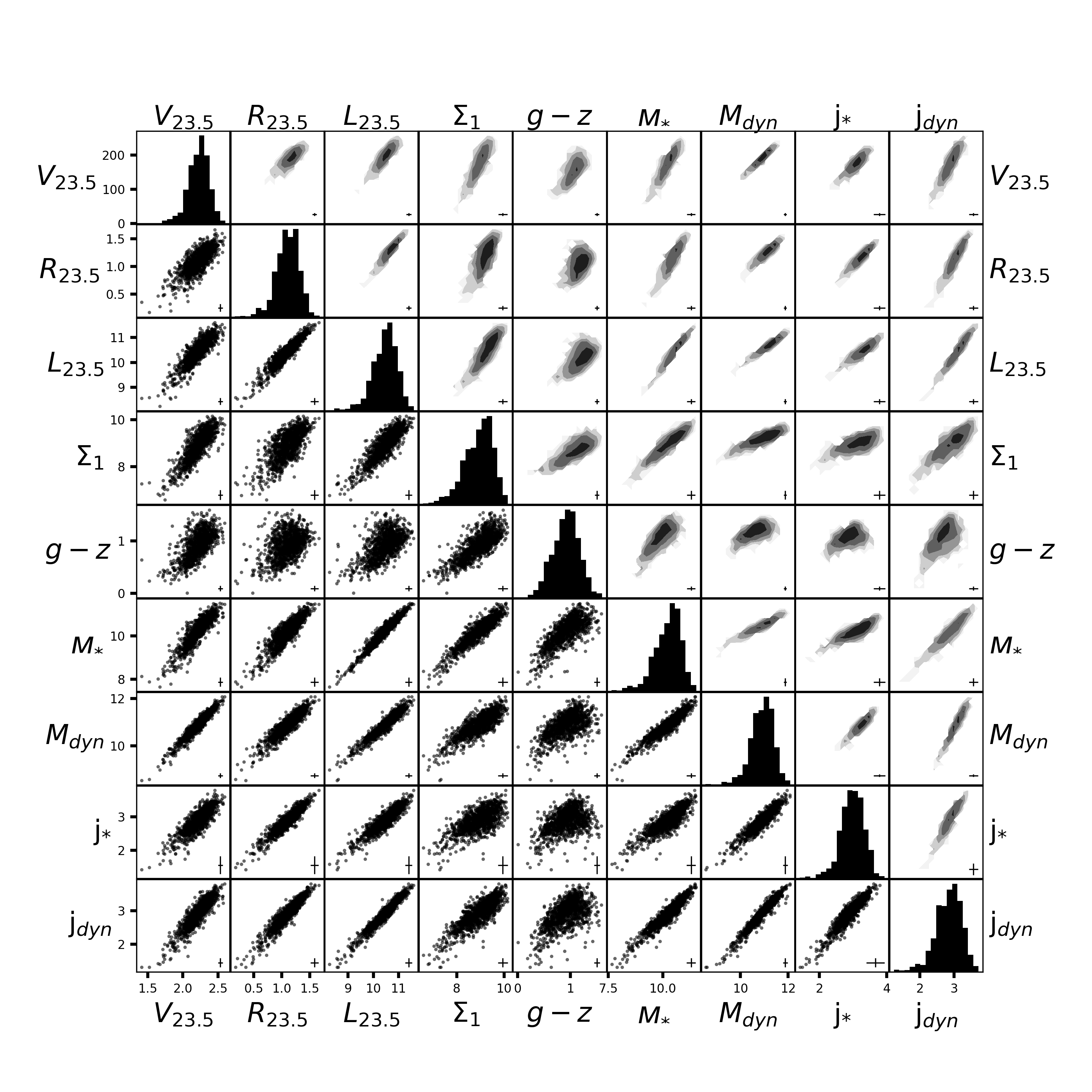
III.3.1
The galaxy size metric used in this analysis corresponds to the isophotal radius, converted to a physical radius using the distance for each galaxy. All sizes in this paper are measured in the band as described in Section III.1. This size metric yields minimal scatter in various scaling relations (Hall et al. 2012; Trujillo et al. 2020a). Incidentally, the radius measured at the band corresponds to a median stellar density of with a quartile range of . The radius advocated by Trujillo et al. 2020a thus samples radii larger than . Both size metrics produce an equally tight size - stellar mass relation (Trujillo et al. 2020b). The range of stellar surface densities for also matches closely the predicted critical gas surface density for star formation in Schaye 2004.
is used as the metric at which all other parameters are measured, except which is measured at (Section III.3.6). It is thus essential that the Bayesian intrinsic scatter model can account for correlated uncertainties, as many variables share at some point in their calculation. is calculated as:
| (6) |
where is the isophotal radius in radians, taken directly from the surface brightness profile. is the distance in parsecs, and is the inclination correction factor (see Section III.4).
III.3.2
The total luminosity in the band, integrated to , is used as a standard metric for the total brightness of a galaxy. The luminosity is computed from a curve of growth, which is itself the integral of a surface brightness profile. Thus, all uncertainties related to zero-point calibrations and isophote uncertainties are carried forward. is calculated as described in Equation 7 below:
| (7) |
where is the solar absolute magnitude calibration, is the apparent magnitude in the band at , and is the inclination correction factor (see Section III.4). We adopt as our preferred luminosity over other metrics, such as the last point in the light profile or extrapolating to infinity, both because it is evaluated at a consistent location in the galaxy profile and it encompasses most of the total light. For comparison, the total light evaluated at the last point of the profile is on average (median) only greater than .
III.3.3
The rotation velocity of each galaxy is computed at the radius and corrected for inclination with the factor and for redshift broadening with the factor, where is the heliocentric velocity of the galaxy divided by the speed of light. Our measurement of uses a fit of the Courteau 1997 multiparameter model to the observed rotation curve. For rotation curves that do not extend to , the fit is extrapolated out to the required radius. A substantial of the PROBES rotation curves require extrapolated estimates for , although over half of these extrapolations are less than beyond the last point in the rotation curve. Once extracted, the velocity is corrected for inclination and redshift broadening as indicated in Equation 8.
| (8) |
where is the observed velocity computed from the Courteau 1997 model, is the systematic velocity which is one of the model fit parameters, is the inclination in radians, and is the heliocentric redshift. All PROBES galaxies are relatively nearby, and the respective redshift corrections (and their uncertainties) are quite small.
III.3.4
Colours for PROBES galaxies are computed as the difference of the and band magnitudes measured at in the DESI-LIS photometry processed as described in Section III.1. We choose colour over (which can also be measured from the DESI-LIS) for its longer baseline and low measurement error. Colours are useful as inputs to colour mass-to-light transformations (Taylor et al. 2011; Conroy 2013; Roediger & Courteau 2015; Zhang et al. 2017; García-Benito et al. 2019) and can be used to construct scaling relations on their own. The colours are calculated as:
| (9) |
where is the apparent magnitude in the band, is the apparent magnitude in the band, and is the inclination correction factor. While the and band magnitudes may be corrected independently first and then have both corrections added to the colour, we have found that the two corrections were highly correlated. It is therefore more accurate in the classical framework to use a single correction factor.
III.3.5
Stellar masses are calculated using the band luminosity (Section III.3.2) and colour (Section III.3.4) input to the Roediger & Courteau 2015 colour to mass-to-light transformations (based on the Bruzual & Charlot 2003 stellar population model). A random error of is assumed for mass-to-light transformations (Roediger & Courteau 2015, see Sec. 4.1 of). Errors on colour/luminosity measurements are propagated separately. For the mass range of most galaxies in PROBES, the Roediger & Courteau 2015 mass-to-light transformations are consistent with other transformations such as Zhang et al. 2017. Numerous uncertainty factors affect stellar mass estimates and are described in the luminosity and colour sections (Sections III.3.2 and III.3.4) Equation 10 expresses the stellar mass calculation.
| (10) |
where is the mass-to-light ratio as a function of the colour . The luminosity and colour are taken as the corrected values in this formula, and no further inclination correction is needed. The stellar mass is, by construction, highly correlated with the luminosity and colour; this is challenging to adequately represent in a classical framework.
III.3.6
The quantity refers to the stellar-mass surface density within a radius of (Cheung et al. 2012; Fang et al. 2013; Zolotov et al. 2015; Teimoorinia et al. 2016; Chen et al. 2020b). Our values are computed using band luminosity (out to ), colour (out to ), and the Roediger & Courteau 2015 colour to mass-to-light transformations as detailed in Section III.3.5. Equation 11 details our stellar-mass surface density calculation.
| (11) | ||||
where is the inclination correction for , is the magnitude within , and is the colour within . The determination of the physical radius at requires a distance measurement. Distance and mass-to-light transformation are the most significant sources of uncertainty in . Because of their common dependence on distance, and are strongly correlated even though they are measured at two different fiducial radii. Obtaining measurements within requires galaxies to be well resolved; nearly of the PROBES galaxies have seeing lengths less than , and are therefore sufficiently resolved for the calculation of . We calculate for all galaxies even if is not in principle resolved; the unresolved of the PROBES galaxies shows a small bias of the order of in their residuals for some scaling relations.
III.3.7
We compute the total mass out to using the observed rotation curves corrected for inclination. Equation 12 expresses the total mass calculation, which is simply a combination of results from Equation 8 and Equation 6 using the virial theorem (Binney & Tremaine 2008).
| (12) |
where is the gravitational constant (all other quantities are as defined above). As would be expected, the total mass is highly correlated with velocity and radius; however, it is also correlated with other variables such as luminosity (and stellar mass) since they share distance as a large source of uncertainty. The Bayesian uncertainty method (Section II.3) is especially well suited to handle strong correlations of this kind, such as those that arise in the context of the stellar mass-halo mass relation (Section V.6).
III.3.8
The dynamical angular momentum of a galaxy is a conserved quantity (in isolation), making it an effective lens into the history of galaxy formation. The specific angular momentum removes the trivial correlation between mass and angular momentum, allowing the physical relationship between these parameters to be studied more directly.
The specific angular momentum, , is computed out to by integrating the velocity profile found by fitting the Courteau 1997 multiparameter model. The use of a model, instead of interpolating between galaxy velocity measurements, is more robust to noise, though some angular momentum information may be lost. Note that the largest deviations from the Courteau 1997 model occur near the center of the galaxy where contributions to angular momentum are suppressed by a factor of , so ultimately the model’s favourable behaviour against noise produces more accurate angular momentum measures.
The expression for specific angular momentum is shown in Equation 13:
| (13) |
where is the rotational velocity as a function of radius, corrected for inclination and redshift as in Section III.3.3. and are as described in Sections III.3.1 and III.3.7, respectively. Note that we only use deprojected quantities in this formula and no further inclination correction is required. Because the angular momentum profiles do not level off at , our profiles are sensitive to the choice of cutoff radius. Therefore, our results describe the angular momentum within and not the total angular momentum.
III.3.9
The stellar specific angular momentum is computed by integrating the stellar surface density and velocity out to . As in Section III.3.8, the Courteau 1997 multiparameter model is used to infer the velocity component. Thanks to the fine sampling and high signal-to-noise of our photometry, we can forgo any model fitting and use the interpolated stellar surface density profile () directly from our isophotal fitting solution. The stellar angular momentum in our analysis is calculated as in Equation 14 as follows:
| (14) |
where is the intensity as a function of radius, and is the mass-to-light ratio as a function of radius (we use the same transformations as in Section III.3.5). is the inclination correction factor. The term in the integral is the corrected quantity from Section III.3.1 and the correction factor is assumed to only correct for the inclination dependence of the intensity profile and the mass-to-light profile . As with , the stellar angular momentum profiles do not converge within and thus do not represent the total stellar angular momentum.
III.4 Inclination Corrections
Most galaxy structural parameters, detailed in Section III.3, show some degree of correlation with inclination. Any parameter correlation with inclination is undesirable as fundamental galaxy properties should not depend on their apparent orientation and projection on the sky. In the case of , this dependence can be counteracted by dividing by ; for other parameters, the transformation is not so trivial.
There are three primary sources of inclination dependence: (i) projection (geometric effect) on the sky; (ii) radiative transfer through the distribution of dust and gas in a galaxy, and (iii) stellar population distributions (or really any other spatially varying quantity). Projection effects can often be handled analytically, for example, in the case of surface brightness (Byun et al. 1994). The brightness (or intensity per unit area) of an ideal galaxy taken as a transparent infinite slab will increase with inclination relative to face-on orientation since it is being projected through a larger length of the slab. The increased brightness could be corrected by multiplying the linear flux by in order to recover the face-on value from any inclination (Holmberg 1958; Giovanelli et al. 1994). However, galaxies are not ideal transparent slabs; instead, they have complex dust, gas, and stellar structures whose nature and distribution may vary from galaxy to galaxy. We have attempted to correct surface brightnesses (and thus all subsequent extracted parameters) with a pure geometric correction of . However, this yielded larger scatter estimates for many of our scaling relations. Clearly, more than simple geometric corrections are at play. A more generalized transformation is required to model these effects.
| Index | Model | Inspiration |
|---|---|---|
| (1) | (2) | (3) |
| 0 | Giovanelli et al. 1994 | |
| 1 | Han 1992 | |
| 2 | Tully et al. 1998 | |
| 3 | Maller et al. 2009 |
Note. — Column (1) indexes the inclination correction models. Column (2) gives the model. Column (3) lists the literature source that inspired the correction model. Note that our model may differ from the quoted source, but is conceptually related (see the text for more details). A subscript means that the parameter changes with morphological type.
The ideal form of a generalized inclination correction model is unknown, though many variations have been tried since at least Holmberg 1958 who used a cosec function. The most common approach takes the form detailed in Giovanelli et al. 1994 and included as Model 0 in Table 1 (Burstein et al. 1991; Han 1992; Willick et al. 1995; Tully et al. 1998; Shao et al. 2007; Graham & Worley 2008; Unterborn & Ryden 2008; Cho & Park 2009; Maller et al. 2009; Masters et al. 2010; Devour & Bell 2016; Devour & Bell 2017; Devour & Bell 2019). Other forms have been explored as well (Möllenhoff et al. 2006; Driver et al. 2007; Driver et al. 2008; Shao et al. 2007; Tempel et al. 2010; Yip et al. 2010; Xiao et al. 2012; Kourkchi et al. 2019). The two common parameterizations of inclination dependence rely on a function of either the axial ratio, , or the inclination (from Equation 5). The latter accounts for the thickness of the disk via a (poorly constrained) flattening parameter , while the former does not. Dust-free images of edge-on galaxies show that the values are clearly nonzero and so our modest assumed value (, Hall et al. 2012) should provide a closer approximation to the truth. The factors in Table 1 encapsulate our ignorance about the exact nature of the obscuration in a galaxy as a function of inclination. The nature of obscuration may vary with disk thickness, dust distribution, disk features, and other unknown factors in a galaxy. As such, the coefficients may change for different galaxy types. Han 1992 divided their sample into Hubble type bins before computing their correction factor; however, later studies have used other techniques. Tully et al. 1998 divided galaxies into magnitude bins then used the TFR to reformat the correction factor as a function of velocity (see also Willick et al. 1997). Driver et al. 2007; Driver et al. 2008 and Masters et al. 2010 separated galaxies into “bulgy” and “disky” groups in order to compute their . Maller et al. 2009 tried two subdivision techniques, one based on magnitude and the other based on Sérsic index, while Cho & Park 2009’s corrections used concentration index as a representation of morphology. In their related series of papers, Devour & Bell 2016; Devour & Bell 2017; Devour & Bell 2019 exploited a two-dimensional space of magnitude and colour in infrared bands. The above works establish a consensus that inclination corrections depend on some notion of galaxy “families” with similar properties. However, the range of techniques speaks to the difficulty of finding parameters that are not themselves inclination dependent.
To generalize the concept of inclination correction, we consider a general model that expresses an extracted parameters dependence on inclination. The model may depend on any galactic parameter, in principle, though we restrict our consideration to inclination, velocity, morphological type, and concentration as these are (mostly) independent of inclination themselves. We can then determine an inclination correction by fitting where is the extracted parameter (Section III.3), is inclination, is the rotation velocity, is morphological type, and is the light concentration index. The fit is performed with a least-squares regression, then the inclination correction is taken to be: which corrects to a face-on value33 3 Internal extinction is still present in face-on systems. Its correction would require a wavelength-dependent radiative transfer code. Such a treatment is beyond the scope of the present study.. Any term in the model that does not depend on inclination will ultimately be absent from the correction and is only used for the sake of fitting. For clarity, the coefficients for these “absent” terms are labeled with .
| Model | Coefficient | |||||
|---|---|---|---|---|---|---|
| (1) | (2) | (3) | (4) | (5) | (6) | (7) |
| 0 | 10.40 | 0.91 | 1.08 | 8.87 | 2.91 | |
| 0 | 0.33 | -0.49 | -0.15 | 0.06 | -0.72 | |
| 1 | 10.46 | 0.97 | 1.09 | 9.06 | 2.91 | |
| 1 | -0.10 | -0.58 | -0.31 | -0.30 | -0.96 | |
| 1 | 10.61 | 0.92 | 1.17 | 9.05 | 3.04 | |
| 1 | 0.48 | -0.51 | -0.07 | 0.13 | -0.63 | |
| 1 | 10.39 | 0.89 | 1.09 | 8.72 | 2.93 | |
| 1 | 0.59 | -0.51 | -0.02 | 0.10 | -0.51 | |
| 1 | 10.45 | 0.88 | 1.16 | 8.67 | 3.06 | |
| 1 | 0.89 | -0.26 | 0.16 | 0.35 | -0.25 | |
| 1 | 9.91 | 0.79 | 0.84 | 8.48 | 2.56 | |
| 1 | 0.08 | -0.27 | -0.41 | 0.44 | -1.12 | |
| 2 | 4.29 | -0.65 | -1.34 | 2.63 | -1.59 | |
| 2 | 1.48 | 1.54 | -0.02 | 3.24 | -1.86 | |
| 2 | -0.58 | -0.95 | -0.08 | -1.51 | 0.49 | |
| 3 | 4.29 | -0.65 | -1.34 | 2.63 | -1.59 | |
| 3 | 1.58 | -0.43 | 0.69 | -0.04 | 0.40 | |
| 3 | 1.18 | 1.13 | 0.40 | 2.84 | 1.63 | |
| 3 | 1.48 | 1.54 | -0.02 | 3.24 | -1.86 | |
| 3 | -0.89 | -0.44 | -0.39 | 0.55 | 0.61 | |
| 3 | 0.31 | -0.50 | 0.31 | -2.06 | -0.12 | |
We considered several models to describe inclination correlations; four such models are listed in Table 1 for comparison. Model 0 is a base case where all galaxies are considered, without regard to subdivision by “family.” Model 1 divides galaxies into bins by morphological type and fits the coefficients for each bin. This represents the simplest notion of inclination correction family. Model 2 allows the coefficient on to be a function of velocity (now expressed as ). Note that Tully et al. 1998 fit coefficients to the residuals of a colour-magnitude fit, while we fit the coefficients directly to the extracted parameter. Tully et al. 1998 used the color and the dependence of on inclination was assumed to be negligible. Model 4 is inspired by Maller et al. 2009, who used infrared wavelength photometry and Sérsic indices. However, the TFR indicates that magnitude in any band (and especially infrared bands) is a tight function of velocity, and so we use it in its stead. Similarly, instead of the Sérsic index, we prefer using the model-independent light concentration index . Maller et al. 2009 fitted their data with their Equation 6 for nearly face-on galaxies, and then fitted the residuals with their coefficients from Equation 9 using a minimization. Our Model 4 encodes this two-step residual fitting into a single operation, though it gives no explicit preference to near face-on galaxies at any point. Table 2 lists the coefficients fitted to the models in Table 1.
After fitting the various models, we examined their effects on our suite of galaxy scaling relations. Figure 3 shows the variation of the scatter and slope with each correction model. Only relations involving parameters that were directly inclination-corrected, and velocity, are included for clarity. Relations not included in the figure showed similar variability with the inclination correction model. Applied to our data, these techniques had mixed effects on our scaling relations, alternately increasing and decreasing the slope/scatter of many scaling relations. Ideally, an accurate model should yield a broad scatter reduction for an ensemble of scaling relations. The only model that fits this description is Model 0, which has no notion of galaxy “families” despite the broad range of PROBES galactic properties. Thus our analysis will use Model 0 for projection correction throughout, even though the true correction likely depends on some notion of galaxy family. Our data are likely not sensitive enough to reveal the nature of (putative) galaxy families.
Figure 3 also reveals the challenging nature of inclination corrections and the power of examining many scaling relations simultaneously. This figure shows that any inclination correction model does confer a reduced scatter in some cases and an increased scatter in others. An inclination correction scheme based on the examination of a single scaling relation could easily map to non-intrinsic quantities.
III.5 Bayesian Error Budget
In the Bayesian formalism, all measurements with uncertainties are randomly sampled and refit with the above analysis methods. As a result, a simplistic uncertainty propagation as shown in Appendix A is not possible; instead, the movement of a point can only be traced when a given variable is perturbed. Figure 4 shows the effect of every source of uncertainty in our analysis for a single galaxy. A similar figure could be produced for every galaxy and there would be some variability in the figures as sources of error change in relative significance; however, UGC 12521 exhibits many typical features.
Since the Bayesian method works by resampling all measurements and then recomputing all variables, some variables did not neatly map into Figure 4. Velocity is determined by fitting a rotation curve comprising many measurements that are typically all individually resampled. To produce a clear signal, we instead increased/decreased all of the velocities by . This is unlikely to occur in a true random sampling scenario; the velocity uncertainty in the figure is thus a worst-case scenario. The surface brightness profile data were also adjusted in the same direction by causing the whole profile to shift (in proportion to the surface brightness, SB, uncertainty), again making this a worst-case scenario for the amount of shift in Figure 4. To account for the systematic velocity uncertainty, the profiles were adjusted after fitting the Courteau 1997 multiparameter model. A systemic velocity shift prior to fitting the model would be canceled by the fitting routine.
Figure 4 shows that all scaling relations have some correlated uncertainties, as well as the relative scatter dependencies for each relation. Distance is typically the dominant source of error. Photometric zero-point, mass-to-light ratio, velocity, and axial ratio are also significant contributors. Curvature can also be seen in some scaling relations (i.e. the versus relation); the proper error propagation for those can only be captured in the Bayesian analysis.
Anticorrelated errors, such as those in most relations involving and the axis ratio , contribute to a scatter increase in a manner that cannot be ascertained by classical analysis. The fits in each panel also show that correlated distance errors (and other correlated sources of error) are often closely, but not entirely, aligned with a scaling relation. Because correlated error vectors would not perfectly slide along the relation, a classical analysis would under(over)estimate intrinsic scatter if distance errors are included (excluded).
III.6 Data Quality Cuts
Various data cuts were applied for quality control. Tests in Appendix B suggest that quality cuts based on parameter uncertainty do not bias intrinsic scatter measurements, while cuts based on deviations from a relation (often referred to as “sigma clipping”) drastically bias scatter measurements. Our fitting method (described in Section IV.1) is also robust to quality cuts; note that sigma clipping is never used in our analysis, even as part of our fitting procedure. Further tests on our fitting routine and intrinsic scatter estimators were performed for a variety of data modifications. The fitting algorithm is robust to realistic sampling biases (e.g. magnitude limited data), covariant observational uncertainties, and slightly incorrect estimates of observational uncertainty. See Appendix B for more details.
Table 3 lists the cuts for the removal of a galaxy from our analysis. Multiple cuts may remove the same galaxy so the totals given for each cut cannot be simply added together. Note as well that some cuts may not remove galaxies from the analysis; however, they may be used for the Bayesian intrinsic scatter calculations if the random sampling generates a pathological galaxy sample.
Starting with 1396 galaxies, we apply our data quality cuts to give 1152 high-quality galaxy samples. Note that we apply our Bayesian analysis to the full original sample, and simulate the effect of our data quality cuts. This means that some galaxies may enter into our Bayesian intrinsic scatter calculation if they are close to the edge of of a data quality cut.
| Variable | Units | N-removed | |||
|---|---|---|---|---|---|
| (1) | (2) | (3) | (4) | (5) | (6) |
| dex | - | - | 0.1 | 65 | |
| deg | 30 | 80 | 10 | 118 | |
| dex | -1 | 2 | 0.15 | 23 | |
| dex | 6.5 | 12 | 0.3 | 28 | |
| dex | 0.8 | 3 | 0.1 | 53 | |
| mag | -0.5 | 2 | 0.2 | 37 | |
| dex | 7 | 12 | 0.4 | 34 | |
| dex | 6 | 10.5 | 0.4 | 22 | |
| dex | 6 | 13 | 0.2 | 76 | |
| dex | 0 | 4.5 | 0.4 | 61 | |
| dex | 1 | 4 | 0.3 | 82 |
Note. — Variables in Column (1) are described in Sections III.3 and III.2. Column (2) indicates the units of the (log/linear) limits. Columns (3) and (4) give a lower and upper bound for each variable. Column (5) gives an upper bound on uncertainty. Column (6) reports the number of galaxies cut from PROBES by limits on that variable, though some galaxies may be removed on account of multiple constraints. No value/limit is set for the distance measurements.
IV Results
IV.1 Scaling Relation Fits
Before evaluating the scatter around a scaling relation, we must first fit linear relations to all parameter combinations. However, the choice of regression model can significantly impact the resulting fitted parameters. For the study of galaxy scaling relations, both axes have heteroscedastic uncertainty (often covariant uncertainty) and neither can be considered an independent variable. Furthermore, a nonzero intrinsic scatter is expected to be present in each scaling relation.
Note. — This table is formatted like Figure 2 with results for each relation at the intersection of two variables. The first column gives the -axis parameter for each scaling relation. The second column gives the linear fit parameters where the fit is of the form: . Reading across a row gives every parameter option as the -variable. The diagonal cells are left blank. Parameter uncertainties are determined by Monte Carlo sampling.
Fits are performed using the BCES bisector algorithm of Akritas & Bershady 1996. These are presented in Table 4 which is organized like Figure 2. The BCES bisector algorithm can model covariant heteroscedastic uncertainties, which we extract from our Bayesian error analysis. All scaling relations appear in the table twice to account for forward and inverse relations, though the fits are performed with a BCES bisector and so the forward and inverse fits are compatible. The first column and first row are analogous to axes of a plot, and so for any value in the table, one can look at the column header to get the -axis and the row variable to get the -axis. The uncertainties presented here include only random errors computed from the Bayesian method and so correspond to the posterior. They do not account for the systematic errors that result from galaxy sample selection or the choice of model. As will be seen in Section V, systematic errors are the dominant source of discrepancies when scaling relation fits from independent studies are inter-compared.
The resulting fits include a large number of known scaling relations. These include relations such as stellar mass - luminosity that are too strongly correlated to be used for testing galaxy formation models. While our values agree well with the literature (see Section V), there is a great variety in intercepts due to parameter choices making their comparison more challenging.
IV.2 Intrinsic Scatter of Scaling Relations
| j∗ | jdyn | |||||||||
|---|---|---|---|---|---|---|---|---|---|---|
| j∗ | ||||||||||
| jdyn | ||||||||||
Note. — This table is formatted like Figure 2 with results for each relation at the intersection of two variables. Each row gives every possible -axis combination for a given -axis. is the observed forward scatter, is the Bayesian intrinsic scatter (see Section II.3), and is the classical intrinsic scatter (see Section II.2). Uncertainty estimates for and are determined by bootstrap sampling; for , the uncertainty is taken from the posterior as the credible interval. The superscript number is the positive value, and the subscript is the negative value. The diagonal cells are left empty.
The intrinsic scatters for all scaling relations under consideration are given in Table 5 in a format similar to Table 4. All scatters are reported as the forward scatter for each parameter combination. Observed scatters () are computed as half the to quartile range of the residuals, which is similar to a standard deviation except more robust to outliers. Bayesian scatters () are computed following Sections II.3 and II.4 with uncertainty determined from the posterior. Classical scatters () are computed following Section II.2 with uncertainty determined by the bootstrap method and taking the to quartiles to get asymmetric uncertainties.
Combining Tables 4 and 5 yields an orthogonal scatter via . The Bayesian intrinsic orthogonal scatter can be used to determine the tightest relation for each variable; however, some tight relations can be considered trivial if the variables depend on each other. The relations , , , , and are deemed trivial in that sense. The tightest relations for each parameter are then found to be: ; ; ; ; ; ; ; ; and , with some parameters having multiple equally tight relations. It is perhaps not surprising that the TFR and stellar TFR are on the list of tightest relations. However, the other tight relations on this list also warrant a closer examination.
Another interesting aspect of Table 5 is the fraction of total scatter, which is intrinsic. The intrinsic scatter fraction is computed in quadrature as where our Bayesian results are used for the intrinsic scatter. Most relations have intrinsic scatters ranging from 70 to 90 percent, with a few relations spanning greater extremes. The , , and relations, also found in our list of tightest scaling relations, have nearly 100 percent intrinsic scatter, making them ideally suited for comparisons with galaxy formation models.
To facilitate intuitive comparisons between scaling relations, Figure 5 presents the slope data from Table 4 and the scatter data from Table 5 graphically. The scatters are represented by ellipticity, which is set to the orthogonal scatter; thus, the forward and inverse versions of each relation are represented by an ellipse of the same thickness. All axes are in dex except which is expressed in magnitude; the latter is converted into dex (dividing by 2.5) before plotting to allow for better visual comparison. generally produces the broadest relations, though it does have a tight nontrivial relationship with .
The orange dashed lines represent cases where the classical intrinsic scatter is negative, as is seen in several cases. Most of these negative classical intrinsic scatter relations display a large covariance caused by one axis being strongly dependent on the other, the , , and relations being the clearest examples. Other cases where the classical uncertainty is negative are due to a shared variable that dominates the uncertainty in each axis, such as the , , and relations. These are all cases where the shared distance uncertainty dominates the covariance, rather than the dependence of one variable on the other. While the possibility of a negative intrinsic scatter is a problematic aspect of a classical analysis, this can sometimes be rectified by identifying the shared uncertainty and simply omitting it from an uncertainty propagation. More sinister are cases where the covariance is not strong enough to cause a negative intrinsic scatter and may remain unnoticed. For example, all of the variables in this analysis share a covariance with inclination due to the internal extinction corrections (see Section III.4; the rotational velocity correction also involves ).
Several qualitative results become apparent upon inspection of Table 5 and Figure 5. Foremost is that the Bayesian intrinsic scatters tend to be larger than the classical estimates. This general result comes from the ability of the Bayesian method to account for covariant uncertainties, which Figure 4 shows are very common. All parameters, except and , depend on distance and gain much of their observational uncertainty from distance errors; any relation with two distance-dependent parameters will thus have a large source of correlated error, which Appendix B shows as a critical point of failure for the classical method. Without exception, inclination is a covariant source of uncertainty in all scaling relations studied in this work; though its effect is smaller than distance uncertainty, Appendix B indicates that even a small covariance can impact classical error propagations. These covariant sources of error contribute less scatter to a relation than the naive classical method assumes. Therefore, the Bayesian method ultimately returns a higher intrinsic scatter value. The effect is most pronounced for and where nearly all classical intrinsic scatter measurements for their scaling relations return negative values. This is not too surprising as these are composite quantities that depend on many factors and so have many source of error to combine.
Another noticeable trend in Table 5 is that the credible intervals for the Bayesian intrinsic scatter values are smaller than the confidence intervals for the classical method. This effect is most significant when the classical intrinsic scatter estimates approach (or cross) zero. In the region around zero scatter, classical estimates are more unstable resulting in the larger uncertainty on the intrinsic scatter. The behaviour of Bayesian intrinsic scatter estimates around zero is better defined, thanks in part to priors that prevent estimates from crossing that threshold. Therefore, the Bayesian intrinsic scatter estimates will be biased high on average. However, they will also typically be closer to the true value than classical estimates (this is generally true of Bayesian methods, also see Appendix B). An inadequate choice of model can also bias both Bayesian and classical intrinsic scatter estimates. For instance, a poorly chosen inclination correction model will typically bias scatter measurements (and therefore intrinsic scatter estimates) higher than their true value. These systematic effects are not reflected in the uncertainty ranges in Table 5 which only shows the random component.
Some specific cases in Figure 5 stand out. The and versus relations and most relations involving colour have similar intrinsic scatter predictions for the Bayesian and classical analyses. These are the cases where most sources of uncertainty are not shared between each axis; it is no coincidence that and colour are in all such relations as they are distance independent (which is a major source of correlated uncertainty). The relation for which the Bayesian and classical methods disagree is vs. which Figure 4 shows has inclination as a large anti-correlated source of error. Anticorrelated errors have a stronger impact on the Bayesian algorithm than the classical method. The Bayesian algorithm cannot in fact assign a zero intrinsic scatter to a relation; one would instead have to perform a Bayes factor analysis to compare the zero and nonzero intrinsic scatter models. This analysis would operationally be similar to our intrinsic scatter calculation, but a detailed description is beyond the scope of this paper.
Figure 5 shows a comparison of many scaling relations by orthogonal scatter. One can read across a row of the figure and see all cases with a single variable as the -axis. A discussion of the generalized applications of these relations, as standard candles for instance, is beyond the scope of this paper, though the format of Figure 5 is conducive to exploring new relationships.
These broad trends indicate the necessity of using Bayesian intrinsic scatter measurements instead of classical techniques. Differences between the two methods extend beyond the trivial second-order effect, but involve systematic and significant departures. We examine specific scaling relations more closely in Section V, and compare our results to the literature.
V Discussion
This section presents a comparison of some of our results with literature values. This exercise demands special attention since structural parameters are rarely measured in matching fashion from study to study. In Table 6 we present our literature comparisons for a few well-studied scaling relations as a subset of those relations presented in Tables 4 and 5. Whenever possible, we perform a unit conversion to units used in our analysis (for example instead of magnitudes), detailing our transformations in the relevant subsection when these are nontrivial. Bandpass transformations were not applied; instead, we report the published values and indicate the wavelengths in which the linear fit parameters were originally measured. Some parameters, such as luminosity, size, and colour, will be greatly affected by the choice of bandpass; others, such as stellar mass, central stellar surface density, and stellar angular momentum, are in principle bandpass independent. However, systematic errors due to the choice of mass-to-light transformations may exist. Comparing scaling relations based on bandpass-dependent quantities, such as the TFR, for different studies thus requires additional care.
Coupled with our analysis technique to evaluate intrinsic scatters, we can achieve higher precision in our estimates than previous (individual) analyses have allowed. However, each relation deserves individual attention in order to fully realize its connection with galaxy formation and evolutionary models. This section focuses on empirical (observational) results; detailed comparisons with simulations are beyond the scope of this paper. The scaling relations examined briefly below set the stage for more detailed investigations elsewhere.
| Source | size | velocity | band | fit method | N | |||
|---|---|---|---|---|---|---|---|---|
| (1) | (2) | (3) | (4) | (5) | (6) | (7) | (8) | (9) |
| Tully-Fisher relation: | ||||||||
| This work | H | 2 bisector | 1152 | |||||
| Tully & Fisher 1977 | HI W | visual | 18 | |||||
| Pierce & Tully 1988 | 0.1 | HI W | OLS | 26 | ||||
| Courteau 1997 | 0.2 | H | OLS | 304 | ||||
| Verheijen 2001 | 0.12 | HI | IOLS | 21 | ||||
| Pizagno et al. 2005 | H | OLS+ | 81 | |||||
| McGaugh 2005 | HI | OLS | 181 | |||||
| Courteau et al. 2007 | H | ODR | 1303 | |||||
| Pizagno et al. 2007 | H | OLS+ | 162 | |||||
| Avila-Reese et al. 2008 | 0.195 | HI W | ODR | 76 | ||||
| Saintonge & Spekkens 2011 | HI W | ODR | 3655 | |||||
| Reyes et al. 2011 | 0.22 | H | IOLS+ | 189 | ||||
| Hall et al. 2012 | 0.27 | 0.15 | HI W | ODR | 668 | |||
| Bradford et al. 2016 | HI W | Kelly 2007 | 930 | |||||
| Ponomareva et al. 2017 | HI | ODR | 32 | |||||
| Ouellette et al. 2017 | H | OLS bisector | 46 | |||||
| Stellar Tully-Fisher relation: | ||||||||
| This work | H | 2 bisector | 1152 | |||||
| Pizagno et al. 2005 | H | OLS+ | 81 | |||||
| Avila-Reese et al. 2008 | 0.21 | HI W | ODR | 76 | ||||
| Dutton et al. 2010 | H | OLS | ||||||
| Reyes et al. 2011 | 0.20 | H | OLS+ | 189 | ||||
| Hall et al. 2012 | 0.305 | 0.281 | HI W | ODR | 668 | |||
| Bradford et al. 2016 | HI W | SDSS | Kelly 2007 | 930 | ||||
| Ouellette et al. 2017 | H | OLS bisector | 46 | |||||
| Lapi et al. 2018 | 3.42 | 0.08 | mixed | OLS | 546 | |||
| Aquino-Ortíz et al. 2020 | 0.20 | mixed | MaNGA | 2 | 200 | |||
| Size-velocity relation: | ||||||||
| This work | H | 2 bisector | 1152 | |||||
| Courteau et al. 2007 | 0.17 | 0.15 | H | ODR | 1303 | |||
| Avila-Reese et al. 2008 | 0.290 | HI W | ODR | 76 | ||||
| Saintonge & Spekkens 2011 | 0.11 | HI W | ODR | 3655 | ||||
| Hall et al. 2012 | 0.152 | 0.146 | HI W | ODR | 668 | |||
| Ouellette et al. 2017 | 0.137 | H | OLS bisector | 69 | ||||
| Lapi et al. 2018 | 1.04 | 0.04 | mixed | OLS | 546 | |||
| Size-luminosity relation: | ||||||||
| This work | 2 bisector | 1152 | ||||||
| Courteau et al. 2007 | 0.14 | 0.13 | ODR | 1303 | ||||
| Avila-Reese et al. 2008 | 0.201 | ODR | 76 | |||||
| Saintonge & Spekkens 2011 | 0.05 | ODR | 3655 | |||||
| Hall et al. 2012 | 0.076 | 0.060 | ODR | 668 | ||||
| Arora et al. in prep. | ODR | 2500 | ||||||
| Size-stellar mass relation: | ||||||||
| This work | 2 bisector | 1152 | ||||||
| Shen et al. 2003 | OLS | 99,786 | ||||||
| Pizagno et al. 2005 | OLS+ | 81 | ||||||
| Fernández Lorenzo et al. 2013 | SDSS | OLS | ||||||
| Lange et al. 2015 | OLS | 6151 | ||||||
| Ouellette et al. 2017 | 0.15 | OLS bisector | 69 | |||||
| Lapi et al. 2018 | 0.23 | 0.05 | OLS | 546 | ||||
| Wu et al. 2020 | F814W | |||||||
| Trujillo et al. 2020b | 464 | |||||||
| Arora et al. in prep. | ODR | 2433 | ||||||
| Stellar-to-halo-mass relation: | ||||||||
| This work | H | 2 bisector | 1152 | |||||
| Reyes et al. 2011 | 0.26 | H | OLS+ | 189 | ||||
| Ouellette et al. 2017 | 0.342 | 0.31 | H | OLS bisector | 69 | |||
| Lapi et al. 2018 | 1.08 | 0.08 | mixed | OLS | 546 | |||
| -Stellar mass relation: | ||||||||
| This work | 2 bisector | 1152 | ||||||
| Barro et al. 2017 | 0.25 | CANDELS | 1328 | |||||
| Woo & Ellison 2019 | 0.86 | 0.24 | OLS | |||||
| Chen et al. 2020a | 0.93 | MaNGA | OLS | 3654 | ||||
| Arora et al. in prep. | ODR | 2433 | ||||||
| Specific angular momentum-mass relation: | ||||||||
| This work | H | 2 bisector | 1152 | |||||
| Takase & Kinoshita 1967 | 18 | |||||||
| Zasov & Rubtsova 1989 | HI W, | 34 | ||||||
| Specific stellar angular momentum-stellar mass relation: | ||||||||
| This work | 2 bisector | 1152 | ||||||
| Romanowsky & Fall 2012 | 0.22 | OLS | 64 | |||||
| Cortese et al. 2016 | 0.18 | SAMI | 106 | 86 | ||||
| Posti et al. 2018 | 0.19 | m | ODR | 92 | ||||
| Lapi et al. 2018 | 0.50 | 0.05 | OLS | 546 | ||||
| Sweet et al. 2018 | mixed | 106 | 91 | |||||
| Mancera Piña et al. 2021 | m | ODR | 132 | |||||
Note. — Column (1) gives the literature source of the scaling relation. Column (2) reports the slope and its uncertainty. Columns (3) and (4) give the forward observed and intrinsic scatter, respectively. In some cases for Columns (2)-(4), the values were transformed from their published value for consistency to ensure uniform units/meaning. Column (5) gives the choice of size metric, if relevant for that relation. Column (6) gives the velocity metric, if relevant, where “HI W” is the HI line width, and the velocity subscripts , refer to the isophotal radius, 2.2 disk scale lengths, of total light, a flat average, and the maximum radius available, respectively. Column (7) gives the bandpass for each measurement, when relevant. In some cases, the original survey from which the photometry was taken is indicated instead of a single bandpass. Column (8) gives an indication of the fitting method. This should be taken as a broad category; see the original article for more information. Where ODR, OLS, IOLS, OLS refer to orthogonal distance regression, ordinary least-squares regression, inverse ordinary least-squares regression, and ordinary least-squares with nonzero intrinsic scatter, respectively. Column (9) gives the number of galaxies in each fit. Dots [] mean that no data are available. If multiple relations were available from a given source, the most relevant version was selected for comparison ( band, local universe, measurements at , bisector fit, late-type galaxies, etc.). This table cannot properly capture the wealth of information found in the literature. Our quoted slope for Lapi et al. 2018 uses the derivative at the pivot point of their fit, ultimately using the value “” from their Table 1; see the original paper for details.
V.1 Tully-Fisher Relation:
The TFR between the rotational velocity, , and total luminosity44 4 The TFR is often expressed in terms of absolute magnitude; in this case a factor of transforms between the slope measurements., , of a spiral galaxy has received considerable attention since its inception (Tully & Fisher 1977; Pierce & Tully 1992; Strauss & Willick 1995; Mo et al. 1998; Verheijen 2001; Courteau et al. 2007; Ferrero et al. 2020, to cite a few). The TFR itself is known to exhibit a wide range of slopes, intercepts, and scatters, depending on the choice of wavelength, sample, and analysis techniques. In their original paper, Tully & Fisher 1977 used photographic photometry and HI line widths for a sample of 18 galaxies to find a photographic ( band equivalent) slope of . Courteau 1997 used band photometry of 304 Sc galaxies and examined many different measures of velocity with two large samples, finding a variety of slopes from up to and forward scatter measurements ranging from 0.14 to depending on the adopted parameters. Later work by Courteau et al. 2007 revealed only weak correlations of the TFR residuals with colour, morphological type, surface brightness, size, and concentration (Zwaan et al. 1995; Courteau & Rix 1999, see also). In their Appendix, Courteau et al. 2007 provide theoretical derivations for the TFR slopes, showing that it can range from three to four depending on various assumptions.
Verheijen 2001 performed a detailed analysis of the TFR parameters against sample, velocity metric, and passband choice, ultimately suggesting that the intrinsic scatter may be zero. Their use of a classical analysis, which systematically underestimates the true value, is likely responsible for their low intrinsic scatter estimate.
The study of 162 spiral galaxies by Pizagno et al. 2007 focused on the scatter of the TFR given combinations of SDSS , and photometric bands; three definitions of global velocity; and variations on extinction corrections, quality flags, and weighting of data points. They again found that the choice of bandpass and analysis method had profound effects on the slope and scatter.
In an attempt to settle one element of this variability, the study by Hall et al. 2012 examined various reference radii for the measurement of luminosity and velocity, consistently finding that the isophotal radius, , measured at the SB level of 23.5 band mag arcsec-2, yields some of the tightest VRL relations (based on a forward scatter analysis).
An extensive examination of bandpass effects on the TFR by Ponomareva et al. 2017 found that 3.6 produces the tightest relation (by orthogonal scatter). Having only 32 galaxies in their sample, random errors were a challenge for Ponomareva et al. 2017 and they found all wavelengths at, or longer than, the band had the same orthogonal scatter to within of each other.
The TFR has been extensively studied, and the works presented in this section are but a small representation of the total literature. Still, we have established general consistency between our analysis and previous, mostly smaller, studies. Some of the above studies have reported measurements for the intrinsic TFR scatter, highlighting its importance for extragalactic studies. Rhee 2000 noted that the true intrinsic scatter is likely larger than classical estimates. With our method, we can finally quantify the effect of covariant uncertainties on the intrinsic scatter of the TFR.
V.2 Stellar Tully-Fisher Relation:
Two variants of the TFR, the stellar and baryonic TFR (STFR and BTFR, respectively), involve a correlation between the rotational velocity and the stellar or total baryonic masses of a galaxy (McGaugh et al. 2000; Verheijen 2001; McGaugh 2005; Hall et al. 2012; Bradford et al. 2016; Ouellette et al. 2017). Note that PROBES has stellar masses, but gas masses are largely unavailable (at the time of writing); therefore, the BTFR is beyond the scope of our research. For a comprehensive review of the BTFR, see Bradford et al. 2016. Here we will only examine the STFR; all STFR values are presented in Table 6.
An operational advantage of the STFR and BTFR over the basic TFR is the elimination of bandpass dependencies. In principle, estimates of the STFR and BTFR should not depend on the methods used to obtain stellar masses and velocities. Therefore, it is surprising that the STFR should exhibit as much, if not more, internal variation in slope and scatter measures than the TFR. Systematic differences in choices of mass-to-light transformations may be at play.
Three studies (Hall et al. 2012; Bradford et al. 2016; Ouellette et al. 2017) have consistent slope measures to ours; however, their scatter values are considerably larger. Differences between the STFR and BTFR are mostly seen at low masses, and sample selection (e.g. yielding varying proportions of low-mass galaxies) may explain these.
V.3 Size-Velocity Relation:
The size-velocity relation (hereafter ) is another tight correlation that can be used as a distance indicator or to constrain galaxy formation models. The slope of the relation is expected to be near one for dark-matter-dominated systems (Mo et al. 1998; Courteau et al. 2007). The PROBES sample includes all of the galaxies studied in Courteau et al. 2007. Despite this significant overlap, we find a larger slope and smaller scatter. These differences in slope and scatter result mostly from using disk scale lengths (Courteau et al. 2007) instead of isophotal radii (this study) and the choice of inclination correction (see Section III.4).
Saintonge & Spekkens 2011 studied the relation for a large collection of Sc galaxies from the SFI++ sample (Springob et al. 2007). Despite the close agreement in slopes, our scatter is considerably larger than theirs. The differences may stem largely from sample selection, with the PROBES sample covering a broader range of morphologies, as well as our velocity measures ( versus HI line width) and photometric band passes ( versus band).
Hall et al. 2012 also explored combinations of velocity, size, and luminosity for 3041 spiral galaxies with HI line widths and SDSS imaging. Their analysis considered different radial definitions, wavelength bands, and sample selection criteria, finding that structural parameters measured at (in their case for the band), yield the tightest scaling relations. In Table 6, we report the results from their highest-quality “sample D,” which has moderate inclinations and well-determined distances. For their less restrictive “sample B,” they find an slope of , which matches our value more closely. Their use of integrated line widths instead of spatially resolved rotation curves should not significantly impact the scatter of the TFR (Courteau 1997). However, resolved rotation curves inform us about the location of the velocity measurement whereas that spatial information is lost with line widths. Other potential sources of discrepancy include the choice of inclination corrections, and their distance calibration (see Hall et al. 2012 Figure 19). Addressing the choice of distance calibration, Hall et al. 2012 found an relation with slope 1.33 and scatter of . An intrinsic scatter for their study can be inferred by taking their reported average uncertainties in size () and velocity () and performing a classical error analysis; this yields an intrinsic scatter of , which is somewhat lower than our intrinsic scatter estimate. Since this value agrees with our classical intrinsic scatter value, the discrepancy is likely due to expected differences between classical and Bayesian scatter analyses.
The Lapi et al. 2018 analysis reported forward and inverse fits to their relation. Using the technique from Isobe et al. 1990, we compute a bisector fit from the forward and inverse fits in Lapi et al. 2018. Their resulting slope is the shallowest among all reported in Table 6. This discrepancy may stem from their use of a disk scale length as the size metric. Courteau et al. 2007 also got a shallower slope and used disk scale lengths as their size metric. The remarkably small scatter of Lapi et al. 2018 is likely connected to their use of stacked profiles.
V.4 Size-Luminosity Relation:
The size-luminosity relation (hereafter ) has the interesting property that both axes are proportional to distance, and therefore distance errors will not significantly contribute to scatter. Although useless as a distance indicator, the residuals of the relation may offer useful comparisons with galaxy formation models without the nuisance of distance uncertainty (Crain et al. 2015).
There is a clear bimodality in results, with Courteau et al. 2007 and Avila-Reese et al. 2008 getting shallow slopes and larger scatters than the other studies. The use of disk scale lengths as the fiducial size metric in these two studies is the most likely source of discrepancy. Sample size (Avila-Reese et al. 2008, e.g.) can also be a factor. Studies that use as their size metric show relative agreement, though classical treatments (Saintonge & Spekkens 2011; Hall et al. 2012) underestimate the intrinsic scatter.
While Hall et al. 2012 did not compute an intrinsic scatter directly, this can be inferred from their reported observational uncertainties. Their reported measurement errors for luminosity and size of and , respectively, imply an intrinsic scatter of based on a classical analysis. Since our data and parameter extraction techniques are similar, the scatter difference is likely due to adopting a classical computation methodology. The classical analysis cannot account for covariances such as the shared effect of a photometric zero-point uncertainty (a positive fluctuation would increase both the luminosity and the size), the shared effect from distance uncertainties, and the shared effect of inclination uncertainties. With so many shared variables, a classical analysis of the intrinsic scatter in the relation is not possible without considering extra covariant terms.
The relation is an ideal testbed for the validation of intrinsic scatter analyses as the variables are strongly correlated, yet the relation itself is nontrivial. The scatter of this relation offers insight into the cosmic diversity of observed galaxies whilst minimizing the influence of observational uncertainties. In fact, our Bayesian analysis finds that essentially all of the scatter is intrinsic as uncertainty contributions are small. It is also a highly reproducible relation, with our results and those of Saintonge & Spekkens 2011 and Hall et al. 2012 being quite similar.
V.5 Size-Stellar Mass Relation:
The size-stellar mass (hereafter ) relation probes several aspects of galactic models including star formation history, angular momentum distribution, and coupling with the dark matter halo. Given the dependence of and on distance, this scaling relation cannot be used as a distance estimator. However, a distinct advantage of the relation over the related relation is the expected independence of on bandpass, making it simpler to compare across observational and numerical studies. As stated previously, the choice of size metric acutely impacts the shape and scatter of the related scaling relations. Studies based on produce tighter relations than other size metrics, and yield slopes consistent with ours (), while those using or consistently get shallower slopes (). Moreover, the intrinsic scatter from Pizagno et al. 2005 is almost twice our value. While Trujillo et al. 2020b used , their intrinsic scatter is slightly smaller than ours, as expected for a classical analysis. As previously stated, Lapi et al. 2018 reported a tight relation, despite using , as a result of their stacking method. The explanation for the larger scatter found by Ouellette et al. 2017 could include small sample size and cluster environment (most other studies sample field environments).
Fernández Lorenzo et al. 2013 considered morphological segregation in their analysis, including early-type galaxies. We have only extracted their slopes for morphologies corresponding to Sb, Sbc, and Sc galaxies as these represent the best overlap with our samples. Table 6 gives their slopes and scatters separated by a “/” character. Shen et al. 2003 also fitted two relations, for low- and high-mass systems (with a transition mass of ). Their use of a circular (Petrosian) half light radius for the relation however explains their extreme slopes and large scatter (Hall et al. 2012).
Overall, the small intrinsic scatter of the relation offers an excellent benchmark for the comparison of observational and/or numerical studies. However, results and their interpretation depend sensitively on the sample selection function and the adopted size metric.
V.6 Stellar-to-Total-Mass Relation:
The stellar-to-total-mass relation (hereafter STMR) plays an important role in understanding the interplay of baryons and dark matter; it is studied across a broad range of scales (see, e.g., Behroozi et al. 2013, for a comparison of several studies). Note that theoretical studies typically examine the Stellar-to-Halo Mass Relation, while observations are limited to STMRs within a finite galactocentric radius (Ouellette et al. 2017). The slope of the STMR changes at a halo-mass scale of (Moster et al. 2010), which represents the star formation efficiency in massive halos. The PROBES sample does not reach the turnover mass range, and we may fit a single power law to our data.
Reyes et al. 2011 and Ouellette et al. 2017 both report STMR slopes that are fully consistent with ours; however, their scatter and intrinsic scatter values are considerably larger. Both studies fit small samples, which increases the uncertainty on their results as a small number of outliers could greatly increase the observed scatter. In the case of Reyes et al. 2011, the increased scatter may also be due to their use of as the radius at which masses are measured, is a variant of the effective radius that is known to produce broader scaling relations. In the case of Ouellette et al. 2017 our analysis techniques are well aligned and so the only other likely explanation is the environment. The Ouellette et al. 2017 sample is taken from the Virgo cluster and our sample is a mix of environments with mostly field galaxies.
Lapi et al. 2018 performed their analysis on stacked data and found an STMR slope and scatter that are considerably lower than ours. Differences are likely explained by their use of stacked data and disk scale length as a size metric.
V.7 -Stellar Mass Relation:
The -stellar mass relation is of great interest to the galaxy formation community. has been empirically shown to be connected with black hole mass, and the transition to a quenched state (Chen et al. 2020b). Unlike other measures such as stellar surface density within the effective radius (), is insensitive to mergers (Szomoru et al. 2012; Barro et al. 2017). Stellar mass is of course sensitive to mergers, and so it is surprising that Barro et al. 2017 find the slope of the -stellar mass relation to be constant as a function of redshift with a slope of (though the zero-point does evolve with time). Our scatter measurements are in close agreement with those of Barro et al. 2017, who reported a scatter of roughly for their star forming galaxies sample, where our value is for a broad range of late-type galaxies.
Woo & Ellison 2019 fit an stellar mass and examine the position of galaxies in the relation and how it is connected to stellar age, specific star formation rate, and metallicity. Specific evolutionary modes are indicated by the apparent paths that galaxies follow in this relation. Fitting only star forming galaxies, they find a slope of 0.86, which is somewhat smaller than our value, though the difference may be attributed to the use of a least-squares fit on the relation. Their scatter measurement of is, however, in excellent agreement with our observed scatter.
Chen et al. 2020a used a large sample of galaxies from the MaNGA (Bundy et al. 2015) survey to find stellar mass to be one of the strongest predictors of radial gradients in stellar population indicators. We find excellent agreement with the Chen et al. 2020a -stellar mass slope of 0.93 for low-mass galaxies (); our reported slope is .
V.8 Specific Angular Momentum-Mass Relation:
Dynamical angular momentum , like dynamical mass, is of special interest to galaxy formation studies since it is a conserved quantity (at least for isolated systems). Angular momentum is also closely tied to dynamical mass through a simple theoretical prediction. Assuming a galaxy is a solid rotating sphere, its moment of inertia will be and total mass is . Computing the angular momentum gives ; the specific angular momentum has (Crampin & Hoyle 1964). Galaxies are, of course, not solid rotating spheres, yet this assumption matches several observational studies, which we discuss below.
The two sources in Table 6 that report the relation have slopes that are consistent with ours; their scatter values are not available. The literature on relation is perhaps not as rich as other relations discussed above, perhaps because of the highly correlated nature of its two variables. Our Bayesian analysis allows for a full accounting of correlations and their effect on intrinsic scatter estimates allowing us to confidently proceed with our analysis. We find a tight relation with a robust slope considerably steeper the simple theoretical predictions above. A possible interpretation is provided by considering the spin-parameter () and energy () of a collapsing halo. This results in a similar power-law relation , though with extra terms (Peebles 1969). If Peebles’s expression represents all relevant parameters, then we must have to roughly reproduce the observed relation.
V.9 Specific Stellar Angular Momentum-Stellar Mass Relation:
The stellar version of the relation involves the complexities of baryonic physics. Nevertheless, the uniformity of empirical results is remarkable (see Table 6) with values for the slope and scatter consistent with ours.
The relative consistency of slope and scatter estimates is quite remarkable given the range of size measures, photometric band passes, and sample sizes used in these various studies. Lapi et al. 2018 consistently report very small scatters due to their stacking method. Our intrinsic scatter is also smaller than those of Posti et al. 2018 and Mancera Piña et al. 2021 possibly due to anticorrelated errors through the axial ratio (see Figure 4). Anticorrelated variables make the Bayesian intrinsic scatter estimates smaller than the classical ones.
Some studies of the relation include a third variable to account for the presence of a bulge (Obreschkow & Glazebrook 2014; Fall & Romanowsky 2018; Sweet et al. 2018). While our Bayesian intrinsic scatter algorithm is well suited for an arbitrary number of dimensions, a multidimensional analysis of scaling relations is beyond the scope of this paper.
V.10 Future Directions
Our analysis has revealed several avenues for future work. The comparison of our results with other studies makes clear that sample selection is a major hindrance, as small samples do not produce reliable results; yet large samples may also exhibit a range of morphologies, masses, environments, etc that can significantly alter final results. Care is required to avoid sampling and selection bias.
We have also (re)visited inclination corrections and their substantial effect on the slope and scatter of galaxy scaling relations. This is discussed in some detail in Section III.4 and will undoubtedly require additional attention on many fronts (empirical, numerical, and theoretical).
Scaling relations also depend sensitively on the choice and definition of the parameters inherent to the relation itself. Most notably, the size metric at which quantities are measured can substantially affect the slope and scatter of the resulting scaling relations (Courteau 1997; Courteau et al. 2007; Hall et al. 2012; Bradford et al. 2016; Trujillo et al. 2020a).
Several scaling relations may have more complicated forms than a single power law, such as the curved STMR, and/or depend on a third parameter such as morphology, bulge/disk ratio, or stellar mass. The Bayesian framework presented in Section II.3 is uniquely suited to address multidimensional analyses. Being entirely based on residuals, the Bayesian method is also well suited for the analysis of intrinsic scatter in nonlinear and multidimensional scaling relations. Exciting avenues for future exploration that could benefit from our Bayesian intrinsic scatter analysis include the evolution of scaling relation scatter against a reference variable or with redshift. The same framework could also account for the changing scatter across a scaling relation, e.g., from the bright to the fainter end. Being entirely forward modeling and residual based, our Bayesian intrinsic scatter analysis is powerful and flexible.
VI Conclusions
We have presented a Bayesian technique for computing intrinsic scatters of arbitrary scaling relations and demonstrated its robustness over the classical first-order method. Because the Bayesian method relies exclusively on forward parameter calculations, no derivatives or inverse functions are required to propagate measurement uncertainties. We have explained the process of estimating Bayesian intrinsic scatters and compared them with “classical” estimates; the former is typically larger than the latter.
We have also applied our method to a suite of observed galaxy scaling relations. For these tests, we use the “PROBES” heterogeneous compilation of 1396 galaxies with spatially resolved H rotation curves and homogeneous photometry extracted by us from the DESI-LIS. Our scaling relations are constructed from all possible combinations of nine structural parameters for late-type galaxies. The resulting scaling relations are homogeneously fit using a BCES bisector. Both Bayesian and classical intrinsic scatter values are then computed for each relation. The agreement between our slope and scatter values and the literature is generally good (Table 6).
Our analysis has yielded the following data products and main results:
- •
A robust set of homogeneously fit scaling relations from a large sample of late-type galaxies covering a broad range of structural properties (Section IV). This includes tables of observed, classical, and Bayesian intrinsic scatters (Table 5), and a detailed comparison with literature values (Section V);
- •
A code to compute Bayesian intrinsic scatters (Appendix C);
- •
An appreciation that Bayesian intrinsic scatters are typically larger than classical intrinsic scatters, as they account for parameter covariances and error propagation through robust fitting techniques (Section II). Most relations have intrinsic scatters ranging from 60 to 90 percent of the total observed value, with a few relations spanning greater extremes.
- •
An appreciation that Bayesian intrinsic scatters are more robust to biases in the data than classical methods (Appendix B);
- •
An identification that the scatter of , , and scaling relations is mostly intrinsic, largely because most observational errors slide along the scaling relations, making some of these relations ideally suited for comparisons with galaxy formation models;
- •
An identification of the tightest scaling relations by intrinsic orthogonal scatter (Section IV.2). For each structural parameter, these relations are: ; ; ; ; ; ; ; ; and , with some parameters having multiple equally tight relations.
- •
A revised discussion on the nature and impact of projection corrections for galaxy structural parameters (Section III.4)
Genuine care is required in order to achieve meaningful analyses of galaxy scaling relations. As discussed in Section V, the parameters associated with any given galaxy scaling relation depend greatly on sample selection and analysis methods. Accurate and representative structural parameters of galaxies, the simultaneous study of multiple scaling relations, and the derivation of robust measures of intrinsic scatter will facilitate comparisons with galaxy formation and evolutionary models. The proper characterization of intrinsic scaling relation scatters ought to help bridge the gap between observations and simulations by removing one of the layers that stands between them.
Appendix A Classical Uncertainty Functions
Here, we report the classical uncertainty functions for all of the extracted parameters in Section III.3. These expressions are determined via Equation 1 and include all sources of uncertainty from Section III for which we could assign a value and calculate derivatives. Table 7 includes expressions for uncertainty for all parameters as used in our analysis.
| Variable | Classical uncertainty |
|---|---|
| (1) | (2) |
Note. — Expressions for classical uncertainty propagation as described in Equation 1. These are computed for all points in each scaling relation and used for the classical uncertainty propagation in Section II.2. The variables are described in the text and Section III.3.
Some variable names appear in Table 7 for the first time and so we describe them here: is the uncertainty on the distance to a galaxy and appears in many of the relations. and are the uncertainty on inclination correction factors for the corresponding variables. is the uncertainty in the surface brightness at the selected radius () and is the local slope of the SB profile at . is the uncertainty on the apparent band magnitude, and is the slope of the curve of growth at the isophotal radius . is the inclination uncertainty (propagation through Equation 5 not shown for clarity), and is the redshift uncertainty. is the uncertainty on the individual velocity measurement at , or the closest point to it. The uncertainty on the systematic velocity was determined by fitting rotation curves with alternative methods (such as an arctan model) and finding typical agreement to within . This value is used as the systematic velocity uncertainty for all galaxies. and are the slopes of the and band growth curves, respectively. is the slope of the mass-to-light ratio as a function of colour, and is the uncertainty on the mass-to-light ratio within set to (Roediger & Courteau 2015, Sec 4.1 of). Similarly, is the uncertainty on the mass-to-light ratio within . is the uncertainty on the magnitude within . is the uncertainty on the intensity at .
Appendix B Testing Data Truncations
Various alterations of the toy model can be made to test the effects of realistic biases in the data. Truncating the data on an axis can represent sampling biases. We test the effect of truncating extreme values on the -axis by setting a lower bound to the axis that removes a given percentage of the data points. Truncating based on uncertainty can represent data quality cuts, and we test the effect of setting an uncertainty threshold that removes some percentage of the data. Truncating based on the residual after fitting a relation can represent sigma clipping, and we test the effect of removing data points with large residuals as well. Shown in Figure 6 are tests for the stability of each method against five types of bias in the data; each test is performed using 1000 trials of the toy model. We compare the relative error between the predicted intrinsic scatter value and the true value as a function of the degree of data bias.
| Bias | 1 | 2 | 3 | 4 |
|---|---|---|---|---|
| (1) | (2) | (3) | (4) | (5) |
| quality cuts | 0.05 | 0.10 | 0.25 | 0.50 |
| sampling bias | 0.05 | 0.10 | 0.25 | 0.50 |
| sigma clipping | 0.01 | 0.02 | 0.03 | 0.05 |
| scaled | 0.02 | 0.05 | 0.10 | 0.25 |
| covariance | 0.01 | 0.02 | 0.05 | 0.10 |
Note. — Table of data modifications from Figure 6 to test the Bayesian and classical intrinsic scatter methods. Column (1) indicates the type of bias applied to the data. Columns (2) - (5) indicate the degree of bias. The numbers in the table have a different meaning for each bias type. Quality cuts, sampling bias, and sigma clipping values refer to the fraction of removed data points. Scaled refers to the factor by which the mock observation uncertainties are scaled relative to their true value. Covariance refers to the degree of extra covariant scatter introduced to the mock observations (note that the toy model intrinsic scatter is approximately 0.13 in the same arbitrary units).
Figure 6 makes clear that scatter analyses are adversely impacted by sigma-clipping methods, since their accuracy and uncertainty bounds are invalidated. This effect becomes significant for the both classical and Bayesian algorithms once as little as of the data are removed. Indeed, sigma clipping eliminates some of the most informative data points from the sample; points close to the relation are consistent with any intrinsic scatter, while those far from the relation that have small uncertainty can only be explained with a nonzero intrinsic scatter. Figure 6 also shows that truncations based on an axis or on uncertainty (as are used in Section III.6) have essentially no effect on either method. We tested truncating up to of the data, and the relative error only increased slightly as would be expected with less data to analyze. Finally, we see that the Bayesian method performs better than the classical method in the ideal toy model (zero bias) by about . The difference is even more pronounced if there is some bias to the data such as correlated errors.
More sinister is the possibility that the observational uncertainties are themselves incorrect. Perhaps a given uncertainty is overestimated as the observer wished to present conservative values, or the uncertainty could be underestimated due to an unknown factor influencing the data. Whatever the cause, biased uncertainties can potentially present a significant barrier to measuring accurate intrinsic scatter values. We test the effect of modifying the uncertainty quality. We also test the impact of correlated uncertainties and verify the statement in Section II that the Bayesian algorithm properly handles correlated uncertainties.
To test for incorrect observational uncertainties, we randomly selected of the data points and scaled their uncertainty by some factor, thus considering both inconsistent data (only half the data is modified) and incorrect uncertainty values. This scaling is done after each data point is perturbed by its uncertainty, so the algorithms will only have access to the scaled (incorrect) values.
To test for correlated uncertainties, an extra uncertainty is added to simultaneously scatter the data in both axes. The classical method considers each axis separately and so the error will be added in quadrature to both axes, while the Bayesian technique includes the new uncertainty in its sampling algorithm as a covariant term.
Figure 6 also shows that both algorithms can handle a small-scale manipulation to the uncertainty values; however the Bayesian algorithm estimate and its uncertainty are consistently more robust. At scaling, the classical algorithm produces an essentially meaningless uncertainty range. The test for covariance in Figure 6 demonstrates, as expected, that the classical method is negatively impacted by this type of uncertainty while the Bayesian method handles it smoothly.
Appendix C Bayesian Intrinsic Scatter Code
Here we present the Bayesian intrinsic scatter code. The Python code below relies on the public numpy (Harris et al. 2020) and scipy (Jones et al. 2001) packages. The code defines the function BayesianIntrinsicScatter which has several arguments described below.
The argument phi_list is a list object where each element contains all of the measurement information for a galaxy (rotation curve, surface brightness profile, distance, etc.) and the associated uncertainties. The galaxy object (elements of the phi_list list) may be formatted in any way that is easiest for the user as the code does not directly interact with them, instead only passing them to other functions. sigma_max is the maximum possible intrinsic scatter value for the prior; typically the total scatter of the scaling relation is used. The two X and Y arguments are functions that take a phi_list element and evaluate the / axes of the scaling relation in question. These functions can return None to indicate that a point has exceeded a data quality cut and should be ignored. Other than returning None, no other assumptions are made about the output of X and Y as they are only passed to user-defined functions. sample_phi_params is a function that takes no arguments and returns any parameters that are needed for the sample_phi function. sample_phi takes parameters from sample_phi_params and an element from phi_list and returns the element resampled about its uncertainty values. For example, the distance measurement would be resampled by a normal distribution about the original measurement with the uncertainty as the standard deviation. relation_f is the function for the scaling relation; it takes as arguments a tuple of parameters, an -axis value, and a -axis value, then returns the residual. relation_f_fit takes a list of -axis values and a list of -axis values and returns the tuple of parameters needed for relation_f. N_samples is the number of times to sample the sample_phi function for each galaxy and should be at least 500 for the posterior to converge. N_sigma is the number of points to evaluate the intrinsic scatter pdf. sigma_min is the minimum value at which to evaluate the intrinsic scatter pdf. nprocs is the number of processors used for the calculations; this can accelerate the Bayesian intrinsic scatter measurement. If the speed up is not needed, one can replace the instances of pool.map with map for the same functionality. min_pass is the minimum number of evaluations out of N_samples that do not return None required for a galaxy to be included in the intrinsic scatter calculation.
While the Bayesian intrinsic scatter calculation is somewhat more complicated than a classical intrinsic scatter analysis, there are some distinct advantages. From a coding perspective, there are only a few functions that need to be defined. The X and Y functions are effectively already needed to construct the scaling relation in the first place. The sample_phi function is relatively simple to construct as it typically only involves sampling normal distributions. Again the relation_f and relation_f_fit functions must already be constructed in order to fit the scaling relation. Contrast this with the classical error analysis where derivatives must be computed for each axis as a function of each input value that has an uncertainty. Once implemented for the first time, the Bayesian intrinsic scatter calculation is actually easier than the classical analysis, though it does take longer to compute.
import numpy as np
from scipy.integrate import trapz
from scipy.stats import norm
from functools import partial
from multiprocessing import Pool

def _pdf(r,s):
    return np.sum(norm.pdf(r, loc = 0, scale = s))

def BayesianIntrinsicScatter(phi_list, sigma_max, X, Y,
                             sample_phi_params, sample_phi,
                             relation_f, relation_f_fit,
                             N_samples = 500, N_sigma = 100,
                             sigma_min = 0.01, nprocs = 4,
                             min_pass = 100):
    pool = Pool(nprocs)
    # array of values at which to evaluate the intrinsic scatter pdf
    S = np.linspace(sigma_min, sigma_max, N_sigma)

    residuals = [[] for n in range(len(phi_list))]
    for r in range(N_samples):
        params = sample_phi_params()
        # Resample galaxy list
        sample = pool.map(partial(sample_phi, params), phi_list)
        # Evaluate scaling relation axes
        XY = zip(pool.map(X,sample), pool.map(Y,sample),
                 range(len(phi_list)))
        XY = list(filter(lambda xy: not None in xy, XY))
        # Fit scaling relation
        fit = relation_f_fit(list(xy[0] for xy in XY),
                             list(xy[1] for xy in XY))
        for xy in XY:
            # Store scaling relation residual
            residuals[xy[2]].append(relation_f(fit, xy[0], xy[1]))

    posteriors = []
    for r in filter(lambda r: len(r) > min_pass, residuals):
        # evaluate the intrinsic scatter pdf for this galaxy
        pdf = np.array(pool.map(partial(_pdf, r), S))

        # normalize pdf to integral 1
        posteriors.append(np.log10(pdf/trapz(pdf, S)))

    # Take product of single galaxy posteriors and normalize
    P_sigmai = np.sum(posteriors, axis = 0)
    P_sigmai -= np.max(P_sigmai)
    P_sigmai = (10**P_sigmai)/trapz(10**P_sigmai, S)

    return S, P_sigmai
References
- Abell et al. (1989) Abell, G. O., Corwin, Harold G., J., & Olowin, R. P. 1989, ApJS, 70, 1
- Akritas & Bershady (1996) Akritas, M. G. & Bershady, M. A. 1996, ApJ, 470, 706
- Andreon & Hurn (2013) Andreon, S. & Hurn, M. 2013, Statistical Analysis and Data Mining: The ASA Data Science Journal, 9, 15
- Aquino-Ortíz et al. (2020) Aquino-Ortíz, E., Sánchez, S. F., et al. 2020, ApJ, 900, 109
- Arora et al. (in prep.) Arora, N., Stone, C., et al. in prep., in prep.
- Avila-Reese et al. (2008) Avila-Reese, V., Zavala, J., et al. 2008, AJ, 136, 1340
- Barro et al. (2017) Barro, G., Faber, S. M., et al. 2017, ApJ, 840, 47
- Behroozi et al. (2013) Behroozi, P. S., Wechsler, R. H., & Conroy, C. 2013, ApJ, 770, 57
- Beifiori et al. (2012) Beifiori, A., Courteau, S., et al. 2012, MNRAS, 419, 2497
- Bender et al. (1993) Bender, R., Burstein, D., & Faber, S. M. 1993, ApJ, 411, 153
- Bernstein et al. (1994) Bernstein, G. M., Guhathakurta, P., et al. 1994, AJ, 107, 1962
- Binney & Tremaine (2008) Binney, J. & Tremaine, S. 2008, Galactic Dynamics: Second Edition (Princeton University Press)
- Bottrell et al. (2017) Bottrell, C., Torrey, P., et al. 2017, MNRAS, 467, 2879
- Bradford et al. (2016) Bradford, J. D., Geha, M. C., & van den Bosch, F. C. 2016, ApJ, 832, 11
- Bradley et al. (2020) Bradley, L., Sipőcz, B., et al. 2020
- Brook et al. (2012a) Brook, C. B., Stinson, G., et al. 2012a, MNRAS, 419, 771
- Brook et al. (2012b) Brook, C. B., Stinson, G., et al. 2012b, MNRAS, 424, 1275
- Bruzual & Charlot (2003) Bruzual, G. & Charlot, S. 2003, MNRAS, 344, 1000
- Bundy et al. (2015) Bundy, K., Bershady, M. A., et al. 2015, ApJ, 798, 7
- Burstein et al. (1991) Burstein, D., Haynes, M. P., & Faber, M. 1991, Nature, 353, 515
- Byun et al. (1994) Byun, Y. I., Freeman, K. C., & Kylafis, N. D. 1994, ApJ, 432, 114
- Chen et al. (2020a) Chen, G., Zhang, H.-X., et al. 2020a, ApJ, 895, 146
- Chen et al. (2020b) Chen, Z., Faber, S. M., et al. 2020b, ApJ, 897, 102
- Cheung et al. (2012) Cheung, E., Faber, S. M., et al. 2012, ApJ, 760, 131
- Cho & Park (2009) Cho, J. & Park, C. 2009, ApJ, 693, 1045
- Conroy (2013) Conroy, C. 2013, ARA&A, 51, 393
- Cooley & Tukey (1965) Cooley, J. W. & Tukey, J. W. 1965, Mathematics of computation, 19, 19
- Cortese et al. (2016) Cortese, L., Fogarty, L. M. R., et al. 2016, MNRAS, 463, 170
- Courteau (1997) Courteau, S. 1997, AJ, 114, 2402
- Courteau et al. (2007) Courteau, S., Dutton, A. A., et al. 2007, ApJ, 671, 203
- Courteau & Rix (1999) Courteau, S. & Rix, H.-W. 1999, ApJ, 513, 561
- Courteau et al. (2000) Courteau, S., Willick, J. A., et al. 2000, ApJ, 544, 636
- Crain et al. (2015) Crain, R. A., Schaye, J., et al. 2015, MNRAS, 450, 1937
- Crampin & Hoyle (1964) Crampin, D. J. & Hoyle, F. 1964, ApJ, 140, 99
- Dale et al. (1999) Dale, D. A., Giovanelli, R., et al. 1999, AJ, 118, 1489
- Devour & Bell (2016) Devour, B. M. & Bell, E. F. 2016, MNRAS, 459, 2054
- Devour & Bell (2017) Devour, B. M. & Bell, E. F. 2017, MNRAS, 468, L31
- Devour & Bell (2019) Devour, B. M. & Bell, E. F. 2019, ApJS, 244, 3
- Dey et al. (2019) Dey, A., Schlegel, D. J., et al. 2019, AJ, 157, 168
- Driver et al. (2008) Driver, S. P., Popescu, C. C., et al. 2008, ApJ, 678, L101
- Driver et al. (2007) Driver, S. P., Popescu, C. C., et al. 2007, MNRAS, 379, 1022
- Dutton et al. (2010) Dutton, A. A., Conroy, C., et al. 2010, MNRAS, 407, 407
- Dutton et al. (2011) Dutton, A. A., van den Bosch, F. C., et al. 2011, MNRAS, 410, 1660
- Efron (1992) Efron, B. 1992, in Breakthroughs in statistics (Springer), 569–593
- Ellison et al. (2020) Ellison, S. L., Thorp, M. D., et al. 2020, MNRAS, 493, L39
- Fall & Romanowsky (2018) Fall, S. M. & Romanowsky, A. J. 2018, ApJ, 868, 133
- Fang et al. (2013) Fang, J. J., Faber, S. M., et al. 2013, ApJ, 776, 63
- Fernández Lorenzo et al. (2013) Fernández Lorenzo, M., Sulentic, J., et al. 2013, MNRAS, 434, 325
- Ferrero et al. (2020) Ferrero, I., Navarro, J. F., et al. 2020, arXiv e-prints, arXiv:2009.03916
- Ferrero et al. (2017) Ferrero, I., Navarro, J. F., et al. 2017, MNRAS, 464, 4736
- Friedman et al. (2010) Friedman, J., Hastie, T., & Tibshirani, R. 2010, Journal of statistical software, 33, 33
- García-Benito et al. (2019) García-Benito, R., González Delgado, R. M., et al. 2019, A&A, 621, A120
- Giovanelli (2013) Giovanelli, R. 2013, Advancing the Physics of Cosmic Distances, 289, 296
- Giovanelli et al. (1994) Giovanelli, R., Haynes, M. P., et al. 1994, AJ, 107, 2036
- Gnedin et al. (2007) Gnedin, O. Y., Weinberg, D. H., et al. 2007, ApJ, 671, 1115
- Graham & Worley (2008) Graham, A. W. & Worley, C. C. 2008, MNRAS, 388, 1708
- Hall et al. (2012) Hall, M., Courteau, S., et al. 2012, MNRAS, 425, 2741
- Han (1992) Han, M. 1992, ApJ, 391, 617
- Harris et al. (2020) Harris, C. R., Millman, K. J., et al. 2020, Nature, 585, 585
- Haynes & Giovanelli (1984) Haynes, M. P. & Giovanelli, R. 1984, AJ, 89, 758
- Holmberg (1958) Holmberg, E. 1958, Meddelanden fran Lunds Astronomiska Observatorium Serie II, 136, 1
- Hopkins et al. (2009) Hopkins, P. F., Hernquist, L., et al. 2009, ApJ, 691, 1424
- Hubble (1926) Hubble, E. P. 1926, ApJ, 64
- Isobe et al. (1990) Isobe, T., Feigelson, E. D., et al. 1990, ApJ, 364, 104
- Jacoby et al. (1992) Jacoby, G. H., Branch, D., et al. 1992, PASP, 104, 599
- Jones et al. (2001) Jones, E., Oliphant, T., et al. 2001, SciPy: Open source scientific tools for Python, [Online; accessed Jan 2021]
- Jonsson et al. (2010) Jonsson, P., Groves, B. A., & Cox, T. J. 2010, MNRAS, 403, 17
- Kelly (2007) Kelly, B. C. 2007, ApJ, 665, 1489
- Kim et al. (2014) Kim, J.-h., Abel, T., et al. 2014, ApJS, 210, 14
- Knebe et al. (2018) Knebe, A., Pearce, F. R., et al. 2018, MNRAS, 475, 2936
- Kourkchi et al. (2020) Kourkchi, E., Tully, R. B., et al. 2020, ApJ, 902, 145
- Kourkchi et al. (2019) Kourkchi, E., Tully, R. B., et al. 2019, ApJ, 884, 82
- Lagos et al. (2018) Lagos, C. d. P., Tobar, R. J., et al. 2018, MNRAS, 481, 3573
- Lambas et al. (1992) Lambas, D. G., Maddox, S. J., & Loveday, J. 1992, MNRAS, 258, 404
- Lange et al. (2015) Lange, R., Driver, S. P., et al. 2015, MNRAS, 447, 2603
- Lapi et al. (2018) Lapi, A., Salucci, P., & Danese, L. 2018, ApJ, 859, 2
- Lelli et al. (2016) Lelli, F., McGaugh, S. S., & Schombert, J. M. 2016, AJ, 152, 157
- Lelli et al. (2017) Lelli, F., McGaugh, S. S., et al. 2017, ApJ, 836, 152
- Maller et al. (2009) Maller, A. H., Berlind, A. A., et al. 2009, ApJ, 691, 394
- Mancera Piña et al. (2021) Mancera Piña, P. E., Posti, L., et al. 2021, A&A, 647, A76
- Masters et al. (2010) Masters, K. L., Nichol, R., et al. 2010, MNRAS, 404, 792
- Mathewson & Ford (1996) Mathewson, D. S. & Ford, V. L. 1996, ApJS, 107, 97
- Mathewson et al. (1992) Mathewson, D. S., Ford, V. L., & Buchhorn, M. 1992, ApJS, 81, 413
- McGaugh (2004) McGaugh, S. S. 2004, ApJ, 609, 652
- McGaugh (2005) McGaugh, S. S. 2005, ApJ, 632, 859
- McGaugh et al. (2016) McGaugh, S. S., Lelli, F., & Schombert, J. M. 2016, Phys. Rev. Lett., 117, 201101
- McGaugh et al. (2000) McGaugh, S. S., Schombert, J. M., et al. 2000, ApJ, 533, L99
- Mo et al. (1998) Mo, H. J., Mao, S., & White, S. D. M. 1998, MNRAS, 295, 319
- Möllenhoff et al. (2006) Möllenhoff, C., Popescu, C. C., & Tuffs, R. J. 2006, A&A, 456, 941
- Mosenkov et al. (2015) Mosenkov, A. V., Sotnikova, N. Y., et al. 2015, MNRAS, 451, 2376
- Moster et al. (2010) Moster, B. P., Somerville, R. S., et al. 2010, ApJ, 710, 903
- Mowla et al. (2019) Mowla, L. A., van Dokkum, P., et al. 2019, ApJ, 880, 57
- Obreschkow & Glazebrook (2014) Obreschkow, D. & Glazebrook, K. 2014, ApJ, 784, 26
- Ouellette et al. (2017) Ouellette, N. N.-Q., Courteau, S., et al. 2017, ApJ, 843, 74
- Peebles (1969) Peebles, P. J. E. 1969, ApJ, 155, 393
- Peng et al. (2010) Peng, Y.-j., Lilly, S. J., et al. 2010, ApJ, 721, 193
- Pierce & Tully (1988) Pierce, M. J. & Tully, R. B. 1988, ApJ, 330, 579
- Pierce & Tully (1992) Pierce, M. J. & Tully, R. B. 1992, ApJ, 387, 47
- Pizagno et al. (2005) Pizagno, J., Prada, F., et al. 2005, ApJ, 633, 844
- Pizagno et al. (2007) Pizagno, J., Prada, F., et al. 2007, AJ, 134, 945
- Ponomareva et al. (2017) Ponomareva, A. A., Verheijen, M. A. W., et al. 2017, MNRAS, 469, 2387
- Posti et al. (2018) Posti, L., Fraternali, F., et al. 2018, A&A, 612, L6
- Price-Whelan et al. (2018) Price-Whelan, A. M., Sipőcz, B. M., et al. 2018, AJ, 156, 123
- Reyes et al. (2011) Reyes, R., Mandelbaum, R., et al. 2011, MNRAS, 417, 2347
- Rhee (2000) Rhee, M. H. 2000, in Astronomical Society of the Pacific Conference Series, Vol. 201, Cosmic Flows Workshop, ed. S. Courteau & J. Willick, 134
- Robotham & Obreschkow (2015) Robotham, A. S. G. & Obreschkow, D. 2015, PASA, 32, e033
- Roediger & Courteau (2015) Roediger, J. C. & Courteau, S. 2015, MNRAS, 452, 3209
- Romanowsky & Fall (2012) Romanowsky, A. J. & Fall, S. M. 2012, ApJS, 203, 17
- Rong et al. (2018) Rong, Y., Li, H., et al. 2018, MNRAS, 477, 230
- Saintonge & Spekkens (2011) Saintonge, A. & Spekkens, K. 2011, ApJ, 726, 77
- Sakai et al. (2000) Sakai, S., Mould, J. R., et al. 2000, ApJ, 529, 698
- Scannapieco et al. (2012) Scannapieco, C., Wadepuhl, M., et al. 2012, MNRAS, 423, 1726
- Schaller et al. (2015) Schaller, M., Dalla Vecchia, C., et al. 2015, MNRAS, 454, 2277
- Schaye (2004) Schaye, J. 2004, ApJ, 609, 667
- Schlegel et al. (1998) Schlegel, D. J., Finkbeiner, D. P., & Davis, M. 1998, ApJ, 500, 525
- Sereno & Ettori (2015) Sereno, M. & Ettori, S. 2015, MNRAS, 450, 3633
- Shai Shalev-Shwartz (2014) Shai Shalev-Shwartz, S. B.-D. 2014, Understanding Machine Learning: From Theory to Algorithms (Cambrige University Press)
- Shao et al. (2007) Shao, Z., Xiao, Q., et al. 2007, ApJ, 659, 1159
- Shen et al. (2003) Shen, S., Mo, H. J., et al. 2003, MNRAS, 343, 978
- Snyder et al. (2015) Snyder, G. F., Torrey, P., et al. 2015, MNRAS, 454, 1886
- Springob et al. (2007) Springob, C. M., Masters, K. L., et al. 2007, ApJS, 172, 599
- Steinmetz & Navarro (1999) Steinmetz, M. & Navarro, J. F. 1999, ApJ, 513, 555
- Stetson (1987) Stetson, P. B. 1987, PASP, 99, 191
- Stone & Courteau (2019) Stone, C. & Courteau, S. 2019, ApJ, 882, 6
- Strauss & Willick (1995) Strauss, M. A. & Willick, J. A. 1995, Phys. Rep., 261, 271
- Sweet et al. (2018) Sweet, S. M., Fisher, D., et al. 2018, ApJ, 860, 37
- Szomoru et al. (2012) Szomoru, D., Franx, M., & van Dokkum, P. G. 2012, ApJ, 749, 121
- Takase & Kinoshita (1967) Takase, B. & Kinoshita, H. 1967, PASJ, 19, 409
- Taylor et al. (2011) Taylor, E. N., Hopkins, A. M., et al. 2011, MNRAS, 418, 1587
- Teimoorinia et al. (2016) Teimoorinia, H., Bluck, A. F. L., & Ellison, S. L. 2016, MNRAS, 457, 2086
- Tempel et al. (2010) Tempel, E., Tamm, A., & Tenjes, P. 2010, A&A, 509, A91
- Tibshirani (1996) Tibshirani, R. 1996, Journal of the Royal Statistical Society: Series B (Methodological), 58, 58
- Tody (1986) Tody, D. 1986, in Society of Photo-Optical Instrumentation Engineers (SPIE) Conference Series, Vol. 627, Instrumentation in astronomy VI, ed. D. L. Crawford, 733
- Torrey et al. (2015) Torrey, P., Snyder, G. F., et al. 2015, MNRAS, 447, 2753
- Trujillo et al. (2020a) Trujillo, I., Chamba, N., & Knapen, J. H. 2020a, MNRAS, 493, 87
- Trujillo et al. (2020b) Trujillo, I., Chamba, N., & Knapen, J. H. 2020b, MNRAS, 495, 3777
- Trujillo-Gomez et al. (2011) Trujillo-Gomez, S., Klypin, A., et al. 2011, ApJ, 742, 16
- Tully & Fisher (1977) Tully, R. B. & Fisher, J. R. 1977, A&A, 54, 661
- Tully & Fouqué (1985) Tully, R. B. & Fouqué, P. 1985, ApJS, 58, 67
- Tully et al. (1998) Tully, R. B., Pierce, M. J., et al. 1998, AJ, 115, 2264
- Unterborn & Ryden (2008) Unterborn, C. T. & Ryden, B. S. 2008, ApJ, 687, 976
- van der Wel et al. (2014) van der Wel, A., Franx, M., et al. 2014, ApJ, 788, 28
- Verheijen (2001) Verheijen, M. A. W. 2001, ApJ, 563, 694
- Willick (1999) Willick, J. A. 1999, in Formation of Structure in the Universe, 213
- Willick et al. (1995) Willick, J. A., Courteau, S., et al. 1995, ApJ, 446, 12
- Willick et al. (1997) Willick, J. A., Strauss, M. A., et al. 1997, ApJ, 486, 629
- Woo et al. (2008) Woo, J., Courteau, S., & Dekel, A. 2008, MNRAS, 390, 1453
- Woo & Ellison (2019) Woo, J. & Ellison, S. L. 2019, MNRAS, 487, 1927
- Wu et al. (2020) Wu, P.-F., van der Wel, A., et al. 2020, ApJ, 888, 77
- Xiao et al. (2012) Xiao, T., Wang, T., et al. 2012, MNRAS, 421, 486
- Yip et al. (2010) Yip, C.-W., Szalay, A. S., et al. 2010, ApJ, 709, 780
- Yung et al. (2019) Yung, L. Y. A., Somerville, R. S., et al. 2019, MNRAS, 490, 2855
- Zasov & Rubtsova (1989) Zasov, A. V. & Rubtsova, T. V. 1989, Soviet Astronomy Letters, 15, 51
- Zhang et al. (2017) Zhang, H.-X., Puzia, T. H., & Weisz, D. R. 2017, ApJS, 233, 13
- Zolotov et al. (2015) Zolotov, A., Dekel, A., et al. 2015, MNRAS, 450, 2327
- Zou & Hastie (2005) Zou, H. & Hastie, T. 2005, Journal of the royal statistical society: series B (statistical methodology), 67, 67
- Zwaan et al. (1995) Zwaan, M. A., van der Hulst, J. M., et al. 1995, MNRAS, 273, L35