Generalized Simple Streaming Codes
from MDS CodesThis research is supported by the J C Bose National Fellowship JCB/2017/000017.
Abstract
Streaming codes represent a packet-level FEC scheme for achieving reliable, low-latency communication. In the literature on streaming codes, the commonly-assumed Gilbert-Elliott channel model, is replaced by a more tractable, delay-constrained, sliding-window (DCSW) channel model that can introduce either random or burst erasures. The known streaming codes that are rate optimal over the DCSW channel model are constructed by diagonally embedding a scalar block code across successive packets. These code constructions have field size that is quadratic in the delay parameter and have a somewhat complex structure with an involved decoding procedure. This led to the introduction of simple streaming (SS) codes in which diagonal embedding is replaced by staggered-diagonal embedding (SDE). The SDE approach reduces the impact of a burst of erasures and makes it possible to construct near-rate-optimal streaming codes using Maximum Distance Separable (MDS) code having linear field size. The present paper takes this development one step further, by retaining the staggered-diagonal feature, but permitting the placement of more than one code symbol from a given scalar codeword within each packet. These generalized, simple streaming codes allow us to improve upon the rate of SS codes, while retaining the simplicity of working with MDS codes. We characterize the maximum code rate of streaming codes under a constraint on the number of contiguous packets over which symbols of the underlying scalar code are dispersed. Such a constraint leads to simplified code construction and reduced-complexity decoding.
Index Terms:
Streaming codes, low-latency communication, packet-level FEC, MDS codes.I Introduction
The availability of a reliable, low-latency communication system is key to many envisaged 5G applications such as telesurgery, augmented and virtual reality. Packet drops are commonplace in a communication network and can arise due to congestion in the network, a weak wireless link or delayed packet arrival. There is need for a communication scheme that can recover from such packet losses in a timely fashion [1]. Packet duplication amounts to using a repetition code and is clearly inefficient. Instantaneous-feedback-based approaches such as ARQ incur an undesired round-trip delay. Streaming codes represent a packet-level Forward Error Correction (FEC) scheme that is both efficient and of low latency.
The study of streaming codes began in [2, 3] where packet-level FEC codes capable of handling an erasure burst within a decoding-delay-window were investigated. Here, encoding is carried out using a packet-expansion framework, a feature that has been retained in the subsequent literature as well, including the present paper. At any time , if is the message packet, then the coded packet , where represents parity. A decoding-delay constraint of , is construed as requiring that be decoded by time .
In [4], a delay-constrained sliding-window (DCSW) channel model was introduced as a tractable deterministic approximation to the more realistic Gilbert-Elliott erasure channel model [5, 6, 7, 8] that is capable of causing burst and random erasures. An DCSW channel imposes a decoding-delay constraint of and permits either at most random erasures or else, a burst of erasures within any sliding window of size time slots, where . Without loss of generality we can set (see [4, 9]). A packet-level code will be referred to as an streaming code if it can recover under decoding-delay from all the admissible erasure patterns of the DCSW channel. An upper bound on the rate of streaming code was derived in [4] and codes achieving this rate for all possible parameters were first presented in [10, 11], thereby characterizing the optimal rate . These initial rate-optimal codes are over a finite field of size exponential in . Currently, the known [9, 12] rate-optimal streaming code constructions have field size that is quadratic in the delay parameter . In [13], rate-optimal streaming codes with rate at least are constructed by combining Maximum Distance Separable (MDS) codes and Maximum Rank Distance codes, but this construction requires a large field size of . Streaming codes for variable size message packets are studied in [14]. Other FEC schemes suitable for streaming setting can be found in [15, 16, 17, 18, 19, 20, 21, 22, 23].
Constructions of streaming codes were originally based on diagonal embedding (DE) of a scalar block code within the packet stream and these codes have a complex structure that could make implementation challenging. Under DE, every diagonal in the packet stream is a codeword in . In [24], a variant of DE called staggered-diagonal embedding (SDE) is introduced which reduces the impact of burst erasures.
In SDE framework a coded packet can contain atmost one symbol from a codeword. Dispersion span is defined as the number of contiguous packets over which code symbols of the underlying scalar code are dispersed. If , then decoding is simplified as each codeword in can be block decoded. For example, in Fig. 1(b) the dispersion span is . Simple Streaming (SS) codes are constructed by SDE with and the underlying scalar code is chosen to be a Reed-Solomon or other MDS code over a finite field of size . MDS codes are widely used in practice and low-complexity algorithms and libraries for encoding and decoding MDS codes are available [25, 26]. The maximum possible rate of a streaming code obtained through SDE with is characterized in [24] and SS codes achieve it. In [27], SDE with dispersion span larger than is explored.
In the present paper, we take the development of streaming codes one step further by allowing within the SDE framework, the embedding of more than one code symbol form the underlying scalar code within a coded packet. We refer to this form of embedding as Generalized SDE (GSDE). Under the condition that the dispersion span satisfies , we characterize the maximum possible rate of an streaming code constructed via GSDE. We show that the underlying scalar code can always be chosen to be an MDS code and hence these codes are simpler to implement. The resultant streaming codes are referred to as Generalized Simple Streaming (GSS) codes. Clearly, the rate of a GSS code can be no smaller than that of a SS code and we characterize the improvement in code rate over than of an SS code.
I-A Motivating Example:
For , the best possible rate of a streaming code is . This rate can be achieved by DE of scalar code presented in [9], see Fig. 1(a). A field of size is required and this code is not easy to implement. The rate achievable using an SS code is , obtained by SDE of MDS code as illustrated in Fig. 1(b). We now describe the construction of an streaming code constructed using GSDE of an MDS code having rate , as shown in Fig. 1(c). Here the code symbols are dispersed across consecutive packets. The embedding can be described using dispersion vector which indicates the number of symbols assigned to successive packets within which the symbols of the MDS codeword are embedded. If denotes the coded packet at time , then is a codeword of , for all . It can be seen that the erasure of any packets or consecutive packets will result in the loss of at most code symbols which is within the erasure-recovery capability of the scalar MDS code. Since here, the decoding-delay constraint is trivially satisfied.
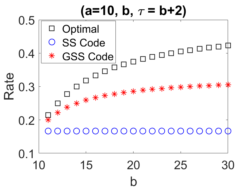
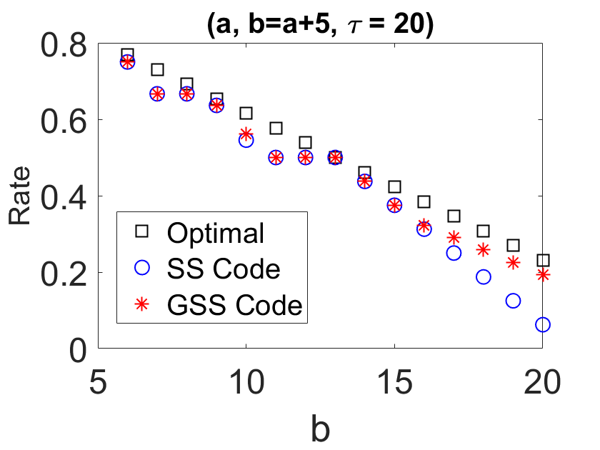
This example illustrates the possibility of improving upon the rate of SS codes by embedding more than one symbol of an MDS codeword within a single packet. Fig. 2 shows the rate of various streaming code constructions for two different parameter settings and the rate gain of GSS code over SS code can be observed in it.
The GSDE framework is formally introduced in Section II and the construction of a GSS code is linked to an interesting combinatorial problem. An upper bound on the rate of streaming codes constructed through GSDE with is derived in Section III. The streaming code constructions are presented in Section IV and it is shown that the rate bound derived in Section III is always achievable.
II Generalized Staggered Diagonal Embedding
Let be an scalar linear code which is systematic, with message symbols appearing as first code symbols. Let be an tuple of non-negative integers with . With out loss of generality we assume . We will refer to as the base code and as the dispersion vector. The parameter is referred to as the dispersion span. Let the coded packet at time be denoted by . Set for all . We say that the packet-level code is constructed by GSDE of base code with dispersion vector if for every ,
|
|
are code symbols of a codeword in . The packet-level code thus obtained has rate . Under the GSDE framework, symbols from a codeword in the base code are dispersed across at most successive packets. Consider a codeword and let be the time indices of the consecutive packets across which this codeword is dispersed. Then, coded packet contains code symbols of . The GSDE framework can be viewed as a generalization of DE and SDE frameworks. For all , for DE, whereas can take values only in for SDE. In GSDE, we allow to be any non-negative integer.
In this paper we focus on the case. This restriction ensures that it suffices to decode each scalar codeword in the conventional block-decoding way, i.e., decode all underlying message symbols after receiving all code symbols belonging to unerased packets. We note that since is permitted for , is equivalent to setting . Throughout the remainder of the paper, when we speak of GSDE, we mean GSDE with . We will now reduce the problem of streaming code construction using GSDE with to a combinatorial problem.
Definition 1.
For example, is a dispersion vector. Now let be an -dispersion vector. Pick an MDS code and construct a packet-level code by GSDE of with dispersion vector . We now argue that the packet-level code thus constructed is an streaming code. An MDS code can recover from erasure of any code symbols. If any arbitrary coded packets are erased, then by (2) at most symbols of any codeword of are erased. If consecutive packets are erased, then once again, no more than code symbols are lost from any codeword, since (3) holds for . Thus (2) guarantees recovery from random erasures whereas (3) assures recovery in the presence of a burst of erasures. The delay constraint is trivially met since symbols of a codeword are spread across consecutive packets. Hence, we have the following Lemma.
Lemma 1.
If there exists an -dispersion vector , then an streaming code of rate can be constructed through GSDE of MDS code with dispersion vector .
We complete the description of relation between dispersion vector and streaming code construction through GSDE by establishing the converse.
Lemma 2.
If GSDE of an base code with dispersion vector results in an streaming code, then is an -dispersion vector, where .
Proof: An code can not recover from more than erasures. Hence, from the -burst erasure and -random erasure correction property of an streaming code, it follows that is an -dispersion vector.
Let denote the maximum rate possible of an streaming codes constructed through GSDE with . It can be inferred from Lemma 2 that the rate of a GSDE based streaming code can not exceed the rate associated to the underlying dispersion vector. Thus, from Lemma 1 and Lemma 2 it follows that can be determined by finding out the maximum rate associated to an -dispersion vector, i.e.,
|
. |
In our search for maximum rate under GSDE, it suffices to restrict our attention to MDS codes. This can be seen as follows. Let be an scalar code that is not an MDS code. Consider an streaming code of rate constructed by GSDE of using dispersion vector . By Lemma 2, is necessarily an -dispersion vector for some . The GSDE of an MDS code with dispersion vector will result in an streaming code of rate . Thus it is not possible to outperform an MDS base code in terms of rate.
We next state our main result, which is the characterization of the maximum possible rate of streaming codes constructed via GSDE and with .
Theorem 3.
Let , where . Then, where
III Rate Upper Bound
Theorem 4.
Let , where . If or , then .
Proof: Let be an -dispersion vector with rate . Suppose . Since obeys (3) we have
Hence and therefore when . Proof for remaining parameter ranges can be found in Appendix -A.
To derive rate upper bound for the case , we first show the existence of a maximum-rate dispersion vector having a specific structure.
Lemma 5.
For any valid , there exists an -dispersion vector of rate with for some .
Proof: See Appendix -B.
From Lemma 5, it can be inferred that in order to determine one needs to look at only the -dispersion vectors for which (3) is satisfied with equality for at least one case.
Theorem 6.
Let , where . If and , then , where .
Proof: Let and be an -dispersion vector of rate with . From Lemma 5 such a dispersion vector always exists. Let and
|
|
(4) |
Let , and be such that
| (5) |
Since satisfies (3), we have
| (6) | |||
| (7) | |||
| (8) |
Adding (5), (6), (7) and (8) gives an upper bound on ,
| (9) |
We will now prove an upper bound on to derive an upper bound on the rate. Let for and . Define to be the set of indices of largest elements from set . It is possible to pick elements from as and . We construct a set comprising of elements given by . Note that the sets ’s and are all disjoint by definition. This implies that:
| (10) |
Let such that , then . Let us define:
| (11) |
By the definition of in (4):
| (12) |
As we pick largest element from to get it follows that:
| (13) |
By substituting (11), (12), (2) in (10) it follows that:
| (14) |
We will now show that . From equation (3) we have
Therefore . Substituting this in equation (14) we get
Now using (9), we have Hence .
IV Constructions
In this section we present two dispersion vector constructions. As explained in Section II, streaming codes can be constructed by GSDE of appropriate MDS codes guided by these dispersion vectors.
Construction 7.
Let , where , . We construct dispersion vector as:
| (15) |
Theorem 8.
The dispersion vector defined by (15) is an dispersion vector with and .
Proof: Clearly, . Note that for all . Hence for any with , . It can also be seen that for all .
The rate of above dispersion vector is , which matches with the rate upper bound in Theorem 4 when or . Hence we have the following corollary.
Corollary 9.
If or , then .
The GSDE of suitable MDS code with above dispersion vector results in SS codes presented in [24]. Since all entries of dispersion vector belong to here, GSDE is same as SDE for this case. For example, this dispersion vector construction gives , which is a dispersion vector. Now GSDE of a MDS code with leads to SS code of rate shown in Fig. 1(b). Now we present a dispersion vector whose rate is same as the rate upper bound in Theorem 6 for case.
Construction 10.
Let with , . Set and . We note that and are always non-negative integers. Now we construct dispersion vector as:
| (16) |
Theorem 11.
If and , then the dispersion vector defined in (16) is an -dispersion vector with and .
Proof: By definition . Pick an element subset such that for all . From , it follows that . Then it can be easily seen that , for all with . Now from the definition of we have . Thus, (2) holds for all with . Additionally, it holds with equality for some cases. For any , it is easy to see that . Hence (3) holds with equality for all the cases.
For , the dispersion vector defined in (16) has rate
where . This rate matches with the upper bound in Theorem 6, resulting in the corollary given below and thereby completing the proof of Theorem 3.
Corollary 12.
Suppose and . Then where .
If or , then GSS code is defined to be same as SS code. For , GSS code is obtained through GSDE of appropriate MDS code with dispersion vector defined by (16). Thus, rate of GSS code . Consider example. The dispersion vector given by (16) for this case is , which is a dispersion vector. The resultant GSS code of rate is given in Fig. 1(c).
If , then and . It follows that GSS codes have rate strictly greater than rate of SS codes if and only if . Table I presents some parameters for which GSS code gives rate improvement over SS code. The table also shows field size requirement for those parameters. We note that for GSS codes and hence a finite field of size is sufficient in the worst-case.
| (3,5,5) | 0.375 | 25 | 0.25 | 3 | 0.3 | 9 |
| (4,5,10) | 0.583 | 100 | 0.556 | 8 | 0.56 | 24 |
| (5,8,16) | 0.6 | 256 | 0.545 | 10 | 0.558 | 42 |
| (9,15,15) | 0.318 | 225 | 0.1 | 9 | 0.25 | 27 |
| (10,18,20) | 0.379 | 400 | 0.231 | 12 | 0.297 | 36 |
V Conclusion
Simple streaming codes are generalized here by permitting each packet to contain more than one code symbol from the underlying scalar code. This results in an increase in code rate that is quantified. The generalized streaming codes presented in this paper use MDS code as the underlying scalar code along with conventional block decoding and hence are simpler to implement than rate-optimal streaming codes known in literature.
References
- [1] G. Americas, “5G Services Innovation,” 2019.
- [2] E. Martinian and C. W. Sundberg, “Burst erasure correction codes with low decoding delay,” IEEE Trans. Inf. Theory, vol. 50, no. 10, pp. 2494–2502, 2004.
- [3] E. Martinian and M. Trott, “Delay-Optimal Burst Erasure Code Construction,” in Proc. Int. Symp. Inf. Theory. IEEE, 2007, pp. 1006–1010.
- [4] A. Badr, P. Patil, A. Khisti, W. Tan, and J. G. Apostolopoulos, “Layered Constructions for Low-Delay Streaming Codes,” IEEE Trans. Inf. Theory, vol. 63, no. 1, pp. 111–141, 2017.
- [5] E. N. Gilbert, “Capacity of a burst-noise channel,” Bell system technical journal, vol. 39, no. 5, pp. 1253–1265, 1960.
- [6] E. O. Elliott, “Estimates of error rates for codes on burst-noise channels,” The Bell System Technical Journal, vol. 42, no. 5, pp. 1977–1997, 1963.
- [7] G. Haßlinger and O. Hohlfeld, “The Gilbert-Elliott model for packet loss in real time services on the internet,” in Proc. 14th GI/ITG Conference on Measurement, Modelling and Evaluation of Computer and Communication Systems. VDE Verlag, 2008, pp. 269–286.
- [8] M. Vajha, V. Ramkumar, M. Jhamtani, and P. V. Kumar, “On sliding window approximation of gilbert-elliott channel for delay constrained setting,” CoRR, vol. abs/2005.06921, 2020.
- [9] M. N. Krishnan, D. Shukla, and P. V. Kumar, “Low Field-size, Rate-Optimal Streaming Codes for Channels With Burst and Random Erasures,” IEEE Trans. Inf. Theory, vol. 66, no. 8, pp. 4869–4891, 2020.
- [10] S. L. Fong, A. Khisti, B. Li, W. Tan, X. Zhu, and J. G. Apostolopoulos, “Optimal streaming codes for channels with burst and arbitrary erasures,” IEEE Trans. Inf. Theory, vol. 65, no. 7, pp. 4274–4292, 2019.
- [11] M. N. Krishnan and P. V. Kumar, “Rate-Optimal Streaming Codes for Channels with Burst and Isolated Erasures,” in Proc. Int. Symp. Inf. Theory. IEEE, 2018, pp. 1809–1813.
- [12] E. Domanovitz, S. L. Fong, and A. Khisti, “An explicit rate-optimal streaming code for channels with burst and arbitrary erasures,” pp. 1–5, 2019.
- [13] D. Dudzicz, S. L. Fong, and A. Khisti, “An explicit construction of optimal streaming codes for channels with burst and arbitrary erasures,” IEEE Trans. Commun., vol. 68, no. 1, pp. 12–25, 2020.
- [14] M. Rudow and K. V. Rashmi, “Streaming codes for variable-size arrivals,” in 56th Annual Allerton Conference on Communication, Control, and Computing, Allerton 2018, Monticello, IL, USA, October 2-5, 2018, 2018, pp. 733–740.
- [15] N. Adler and Y. Cassuto, “Burst-erasure correcting codes with optimal average delay,” IEEE Trans. Inf. Theory, vol. 63, no. 5, pp. 2848–2865, 2017.
- [16] D. Leong and T. Ho, “Erasure coding for real-time streaming,” in Proceedings of the 2012 IEEE International Symposium on Information Theory, ISIT 2012, Cambridge, MA, USA, July 1-6, 2012, 2012, pp. 289–293.
- [17] D. Leong, A. Qureshi, and T. Ho, “On coding for real-time streaming under packet erasures,” in Proceedings of the 2013 IEEE International Symposium on Information Theory, Istanbul, Turkey, July 7-12, 2013, 2013, pp. 1012–1016.
- [18] D. Malak, M. Médard, and E. M. Yeh, “Tiny codes for guaranteeable delay,” IEEE Journal on Selected Areas in Communications, vol. 37, no. 4, pp. 809–825, 2019.
- [19] S. Yang and R. W. Yeung, “Batched sparse codes,” IEEE Trans. Inf. Theory, vol. 60, no. 9, pp. 5322–5346, 2014.
- [20] A. Shokrollahi, “Raptor codes,” IEEE Trans. Inf. Theory, vol. 52, no. 6, pp. 2551–2567, 2006.
- [21] A. R. Iyengar, P. H. Siegel, R. L. Urbanke, and J. K. Wolf, “Windowed decoding of spatially coupled codes,” IEEE Trans. Inf. Theory, vol. 59, no. 4, pp. 2277–2292, 2013.
- [22] A. J. Feltström and K. S. Zigangirov, “Time-varying periodic convolutional codes with low-density parity-check matrix,” IEEE Trans. Inf. Theory, vol. 45, no. 6, pp. 2181–2191, 1999.
- [23] S. C. Draper and A. Khisti, “Truncated tree codes for streaming data: Infinite-memory reliability using finite memory,” in 8th International Symposium on Wireless Communication Systems, ISWCS 2011, Aachen, Germany, November 6-9, 2011, 2011, pp. 136–140.
- [24] M. N. Krishnan, V. Ramkumar, M. Vajha, and P. V. Kumar, “Simple streaming codes for reliable, low-latency communication,” IEEE Commun. Lett., vol. 24, no. 2, pp. 249–253, 2020.
- [25] J. S. Plank and K. M. Greenan, “Jerasure: A library in C facilitating erasure coding for storage applications–version 2.0,” Technical Report UT-EECS-14-721, University of Tennessee, Tech. Rep., 2014.
- [26] “Intel Intelligent Storage Acceleration Library,” https://software.intel.com/content/www/us/en/develop/tools/isa-l.html.
- [27] V. Ramkumar, M. Vajha, M. N. Krishnan, and P. V. Kumar, “Staggered diagonal embedding based linear field size streaming codes,” in IEEE International Symposium on Information Theory, ISIT 2020, Los Angeles, CA, USA, June 21-26, 2020, 2020, pp. 503–508.
-A Proof of Theorem 4
Let be an -dispersion vector with rate . Suppose . Let where . Let us set
| (17) |
We first obtain an upper bound on in terms of and . Let , such that
| (18) |
Since satisfies (3),
| (19) | |||
| (20) |
| (21) |
Now we derive an upper bound on and then use it to obtain the rate upper bound. Define for all . From (17) we get
| (22) |
Let be the set of indices of largest elements from . Then by pigeonhole principle,
| (23) |
Let us define
-B Proof of Lemma 5
Lemma 13.
Let be an dispersion vector with rate . Define and suppose . Then there exists an dispersion vector with for some .
Proof: It is always possible to pick a subset with such that for all . Now suppose . Then, it follows that , for all with . Since , doesn’t satisfy (3) with equality for any . This contradicts the fact that is an dispersion vector. Hence,
| (24) |
Define and . Now we will argue that for all . Let with . Assign and . For any ,
Since ,
for all with . We also have
Therefore is an dispersion vector. This dispersion vector has rate , which is a contradiction. Hence,
| (25) |
Suppose , resulting in for all . Then, from (24) we have . It follows from statement of Lemma that . Since and , this results in a contradiction. Therefore is non-empty. We note that and . From (24), we get
| (26) |
Let and . Since and , it follows from (25) that there exists some with . If , then by (25) and (26) we have
which is not possible. Hence, there exists some such that . With this notation we define the new dispersion vector as:
Claim 1
is an dispersion vector with rate .
Proof of Claim 1
Since , is a -tuple of non-negative integers. Now from definition of it follows that
thus satisfying (1). For all ,
Thus satisfies (3).
If for with , then . Otherwise, (2) is violated for . It can be easily seen that
For all such that and ,
For such that and , . This means
for all with and . Thus, (2) holds for .
It is possible to pick an with and , then we have
Thus, is an dispersion vector. This completes the proof of Claim 1.
Since and , it can be easily seen that .