MoSES_2PDF: A GIS-Compatible GPU-accelerated High-Performance Simulation Tool for Grain-Fluid Shallow Flows
Abstract
We introduce a GPU-accelerated simulation tool, named Modeling on Shallow Flows with Efficient Simulation for Two-Phase Debris Flows (MoSES_2PDF), of which the input and output data can be linked to the GIS system for engineering application. MoSES_2PDF is developed based on the CUDA structure, so that it can well run with different NVIDIA GPU cards, once the CUDA vers. 9.2 (or higher) is installed. The performance of the MoSES_2PDF is evaluated, and it is found that the present GPU-CUDA implementation can enhance the efficiency by up to 230 folds, depending on the PC/workstations, models of GPU card and the mesh numbers in the computation domain. Two numerical examples are illustrated with two distinct initial inflow conditions, which are included in two modes of MoSES_2PDF, respectively. In the numerical example of a large -scale event, the 2009 Hsiaolin event, the results computed by two distinct NVIDIA GPU cards (RTX-2080-Ti and Tesla-V100) are found to be identical but tiny deviation is figured out in comparison with the results computed by the conventional single-core CPU-code. It is speculated to be caused by the different structure in the source codes and some float/double operation. In addition to the illustration in GIS system, the computed results by MoSES_2PDF can also be shown with animated 3D graphics in the ANSI-Platform, where the user can interact with 3D scenes. The feasibility, features and facilities of MoSES_2PDF are demonstrated with respect to the two numerical examples concerning two real events.
Keywords GPU-accelerated CUDA GIS-compatible Grain-fluid shallow flows Simulatiom tool
1 Introduction
Many of the geophysical hazardous flows, such as landslides or debris flows, usually take place in mountain area and flow on non-trivial topography. It is clear that the geometry of the topography may have significant impacts on the flow paths. For the sake of hazard assessment, risk management or evaluation of disaster mitigation countermeasures, numerical simulation is commonly a powerful tool for scenario investigation. Hence, it is highly requested to develop an effective tool of high efficiency and high performance for providing useful information concerning the flow behavior, such as the paths, velocity and flow thickness, etc. A successful simulation of hazardous flows on real topography depends on the availability of the digital elevation model (DEM) essential. With the rapidly growing popularity of the UAV and the integrated modern remote sensing technology, the expensive high resolution data, such as the LiDAR-derived DEM or the aerial photos, has become affordable and enriched the Geographic Information System (GIS) a lot. From the viewpoint of scenario investigation, one of the urgent tasks would be the integration of the simulation tools with the GIS as well as with a high efficient computational performance. Numerical simulation based on Physics-based dynamical models can help the quantitative investigation on the impacts caused by the plausible geophysical hazardous flows. However, in addition to the high-resolution DEMs, it also requests expensive computer resources, depending on the resolution and computation domain. The launch of Compute United Device Architecture (CUDA), a parallel computing platform and programming model, provides an econamic solution for speeding up the computational efficiency by means of employing the graphical processing units (GPUs). The computation duration can therefore be shorten to be less than the scenario time. Hence, either computation with real-time illustration or training for model parameters has become achieveable in an efficient way even without expensive computer resources.
In the past decades, many efforts have been devoted to modeling these highly destructive flows. Since these flows are generally thin (measured normal to the basal surface) in comparison with the large extension in the direction tangential to the topographic surface, shallowness assumption and depth-integration are often introduced for reducing the complexity of the model equations as well as of the numerical approach. For the ease of deriving the governing equations, many of the models are given in Cartesian coordinates (Pitman and Le 2005; Li and Duffy 2011, e.g.,), where the topography is added on the horizontal or inclined plane, or in the locally inclined Cartesian-type coordinates (Pudasaini 2012; Pudasaini and Mergili 2019, e.g.,). For an appropriate description of the depth-averaged velocity as well as for the employment of the shallowness assumption, the terrain-fitted coordinate system has been introduced. In addition to the curved-twisted coordinate proposed by Pudasaini and Hutter 2003, the remarkable works for general topography are Bouchut and Westdickenberg 2004; Tai and Kuo 2008; Tai et al. 2012 and Luca et al. 2016. As well, assuming the non-trivial topographic surface to be composed of finite number of triangles, local coordinate system is introduced on each triangular element for reducing the complexity of numerical implementation in a unstructured mesh system (Rauter and Tuković 2018; Tai et al. 2021, see).
Regarding the composition of the flow body, models for hazardous flows can be divided into four categories: a) single-phase model; b) quasi-two-phase models; c) two-phase models; and d) multi-phase approaches. The key issue by the single-phase approach is the introduction of an appropriate rheological relation, which is definitely different to the Newtonian one due to the complex composition. Taking into account the existence of yield stress, models with the Bingham plastic relation (Liu and Mei 1989; Coussot 1997, e.g.,) or with the Herschel-Bulkley law (Huang and Garcia 1998; Ancey 2007, e.g.,) have been suggested. In addition, a generalized visoplastic model is proposed by Chen (1988), covering the models by Bagnold’s model (Bagnold 1954) and Takahashi’s constitutive relation (Takahashi 1978). For the ease of numerical implementation, commercial codes are mainly released based on the single-phase models for engineering purposes. One of the most popular ones is the FLO-2D, initially following the rheological model proposed by O’Brien and Julien 1985; O’Brien and Julien 1988 and improved by many sequential works (O’Brien et al. 1993, e.g.).
The quasi-two-phase or the two-phase models are based on the concept of two-phase mixture. However, in the quasi-two-phase models, the relative velocity between the two constituents is assumed to be very small, so that its impacts are assumed to be insignificant and only one velocity is considered for the conservation of linear momentum (Iverson 1997; Iverson and Denlinger 2001; Pudasaini et al. 2005; Tai and Kuo 2012, e.g.,). Since only one velocity is taken into account, the dynamic behavior of the flow body is similar to a single-phase fluid (if entrainment or deposit at the bottom is not included), and the effects of the concentration are then parametrically (instead of dynamically) considered in the rheological relation. In addition to the type of Coulomb-mixture (Iverson 1997; Iverson and Denlinger 2001), another approach is the quasi-two-phase grain-flow model, widely employed in Japan for engineering applications, e.g., Egashira 1997; Egashira 2007; Nakatani et al. 2008; Liu et al. 2013; Nakatani et al. 2016. Emphasizing the the role of the interstitial fluid on the behavior of flows, the Coulomb-mixture theory has been improved by introducing the non-hydrostatic pore-fluid pressure for the dilatancy effects by the solid constituent (Iverson 2009; Iverson and George 2014).
In the two-phase models, each constituent is described by individual momentum equation and has its own velocity. Hence, the key feature of a two-phase model is the capability of describing the phase separation, which is documented in field surveys and laboratory experiments. To our limited knowledge, the first inspiring two-phase model for debris flows would be Pitman and Le 2005, although the fundamental investigation on two-phase mixture theory for grain-fluid has been made since years (Anderson and Jackson 1967, e.g.,). Based on Pitman and Le 2005, Pelanti et al. 2008 introduced the well-balancing property in the numerical implementation, where the variable topography is included. Pailha and Pouliquen 2009 suggested a two-phase description for the initiation of underwater granular avalanches. Luca et al. 2012 has theoretically considered over-saturated mixtures in coordinate of general topography. The quadratic viscous drag force and virtual mass force are considered in Pudasaini 2012. A two-phase model in two-layer type and taking into account the dilatancy effects can be found in Bouchut et al. 2016, which mainly considers the submarine debris flows, i.e. the upper layer is pure fluid and not thin. With two-layer approach, the partially unsaturated grain-fluid mixtures are modeled by Meng et al. 2017, where a fluid-saturated granular layer is overlaid by a pure granular material. With thermodynamically consistent derivation, models of granular-fluid mixtures with non-hydrostatic pore pressure can be found in Heß et al. 2017; Heß et al. 2019, where the solid phase is assumed hypoplastic. The multi-phase approach can be found in Pudasaini and Mergili 2019, where the flow body is composed of three phases (the coarse and fine solid fractions, and the viscous interstitial fluid), and the model equations are given in the locally inclined Cartesian-type coordinates for describing the flows over a non-trivial topography.
Regarding the GIS-compatible simulation tool, Mergili et al. 2017 introduced a GIS-supported open-source computational framework, r.avaflow, which is developed to link to the open-source GIS package, GRASS GIS. The r.avaflow is based on a two-phase solid-fluid mixture model (Pudasaini 2012), and mass exchange at the basal surface (entrainment or deposition) are taken into account. In addition, r.avaflow allows multiple-model-runs that multiple parameter sets can be simultaneously executed with the parallel processing function. Although it does not shorten the duration for a single run (a parameter set), this facility may help in looking for the optimal parameter set or collecting abundant plausible simulation scenarios. The r.avaflow has been extended for the multi-phase flow model (Pudasaini and Mergili 2019), see Mergili 2014-2020, and several engineering applications are available in Mergili et al. 2020; Baggio et al. 2021.
Although many of the above-mentioned models are with numerical implementation and able to provide satisfactory results, the computation processes are usually very time-consuming and cost a lot of computer resources. In order to improve the efficiency of computation, one may speed up the computing applications by harnessing the power of graphical processing units (GPUs). Although GPU was originally designed for graphics rendering on computers, especial for the illustration of 3D objects, GPU-accelerated high-performance computation has become more and more popular in various scientific fields, such as Artificial Intelligence (AI), machine learning (ML), deep learning (DL) etc. For example, Castro et al. 2011, Brodtkorb et al. 2012, de la Asunción et al. 2013, and Aureli et al. 2020 have proposed GPU-accelerated approach based on the shallow water equations (SWEs), while Dazzi et al. 2019 integrated the GPU-accelerated 2D SWEs code with levee breach mechanism. A GPU-enhanced 2D SWEs code for curved triangular meshes is developed by Wu et al. 2021, of which the scheme is entropy stable and provides high-order accuracy.
However, there is no GIS-compatible and GPU-accelerated simulation tool for two-phase grain-fluid flows yet. Based on the two-phase model by Tai et al. 2019, we developed the GPU-accelerated simulation tool, MoSES_2PDF, which follows the CUDA structure to integrate the GPGPU technology. In addition, the MoSES_2PDF is designed to be GIS-compatible. That is, the input data is in the asc-format and can be directly acquired from GIS systems (ArcGIS, QGIS), and the output results can be transformed into asc-format for illustration in GIS systems. On the other hand, in MoSES_2PDF we also use the GPU graphics rendering functions in OpenGL for 3D numerical results presentation, which combines the computation results with 3D objects to mimic the effect of reality simulation.
In the second section, we brief the grain-fluid model and employed numerical implementation. The introduction of the framework of MoSES_2PDF and its performance with the GPU parallel computation facility are given in Sect. 3, two modes for different initial inflow conditions are designed and three output formats available for results illustration. In the fourth section, two application examples are illustrated, which are two historical events taking place in 2009 in Taiwan. The application potential and the key features of MoSES_2PDF are summarized and highlighted in the concluding remarks.
2 Modeling and Numerical Implementation
2.1 Modeling
In the GIS system, the topography is described by a set of altitudes of terrain locations over a regular horizontal grid, the digital elevation model (DEM). Based on the DEM, a terrain-fitted coordinate system can be introduced in the vertical-horizontal-oriented Cartesian coordinates , where the - and -axis lie on the horizontal plane and the direction of points upwards. The system can be chosen in the way that, e.g., the projections of -axis and -axis on the horizontal plane coincide with -axis and -axis, respectively (cf. Fig. 1). The coordinates between and is related by the transformation matrix , see Tai et al. 2012 or Luca et al. 2016 for details.
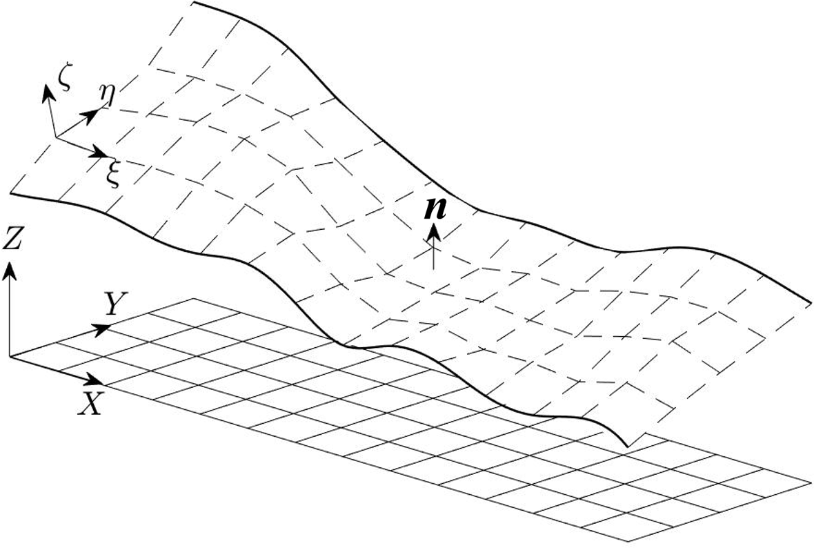
In MoSES_2PDF, the evolution of the flow body is computed by a depth-integrated two-phase grain-fluid model for debris flows over rugged topography (Tai et al. 2019), where the conservations of mass and momentum are taken into account and both of the coordinate systems, and , are used. Hence, there are 6 model equations for the evolutions of the 6 physical quantities, . Here and hereafter, the superscripts “” and “ ” indicate the variables for the solid and fluid constituent, respectively, and the subscript X,Y,Z indicates component in , while ξ,η,ζ for the one in . For a concise description, the employed model equations are not shown here, but presented in A for readers.
Since the flow body is treated as a two-phase mixture, in , and are defined, where denoting the depth-averaged volume fraction and represents the flow thickness measured in the direction normal to the basal topography. In addition, it should be noted that the variables and are the - and -component of the flow velocity projected on the horizontal plane. With the help of the transformation matrix on the basal surface, one can get the flow velocities tangential to the topographic surface.
2.2 Numerical implementation
MoSES_2PDF is developed based on the CUDA structure (CUDA Toolkit vers. 11.0). The employed numerical implementation is same as in Tai et al. 2019, that the balance equations with respect to the solid and fluid constituent are computed separately at each time step, where the anti-diffusive, non-oscillatory central scheme (adNOC, see Kurganov and Tadmor 2000; Kurganov et al. 2007) is used for solving the six differential equations. For details of the numerical implementation, we refer the readers to Tai et al. 2019, in which the code is developed for single-processor (single-core) computation.
The high resolution in space is achieved by utilizing the cell reconstruction, such as the total variation diminishing (TVD), essentially non-oscillatory (ENO) or weighted essentially non-oscillatory (WENO) scheme. And the high-order accuracy in time is carried out by the multi-step Runge-Kutta (RK) method with respect to a semi-discrete formulation given in Kurganov and Tadmor 2000. In MoSES_2PDF, the Minmod TVD slope limiter is adopted and the two-step modified Euler (second-order RK) is employed. As indicated in Kurganov and Tadmor 2000, the time step should be limited by the Courant-Friedrichs-Lewy (CFL) condition with a number of 0.125 and the CFL = 0.1 is set in MoSES_2PDF.
3 Framework of MoSES_2PDF and its Performance
3.1 Framework

3.1.1 Teamwork of CPU and GPU
With respect to the hardware structure, the computational framework of MoSES_2PDF can be divided into two sections, the CPU- and GPU-section, where they have to communicate with each other to complete the operation of computation. Since the data transfer between the sections could be very time-consuming, it is therefore designed in the way to minimize the data transfer as possible, that the CPU-section mainly processes file reading and output, and the rest computational procedures are operated in the GPU-section, cf. Fig. 2.
According to the characteristics of applied numerical scheme, the execution hierarchy of single instruction corresponding to multiple threads (SIMT) is employed as the GPU computing architecture for the purpose of a high efficiency in computation. Besides, most of the calculations are matrix operations, yielding the fact that the memory location of a matrix may cover several blocks, depending on the size of the computational domain (grid numbers). It leads to a hurdle in looking for the global extreme (maximum or minimum) value in the matrices, because the function of global synchronization is not supported in the CUDA parallel-programming model (library). If one uses the type of loop for searching over the whole domain in the CPU-section, the data transfer/collection among the blocks will significantly retard the computational efficiency. Hence, the extreme-value-searching plays a crucial role in efficiency enhancement, and one has to find an effective way for data communication among different blocks. In MoSES_2PDF, we adopt the method of optimizing parallel reduction, proposed by Harris et al. 2007, in the CUDA code to compute the maximum/minimum values in the entire domain. That is, taking the maximum value as example, the maximum value on each block is first figured out, and then they will be transferred to a specified block, in which the global maximum value is identified. In this way, the computation efficiency of the searching process is improved with a significantly higher efficiency than the computation of using the loop type.
3.1.2 Operation of MoSES_2PDF
The operation of MoSES_2PDF consist of four main stages (cf. Fig. 2):
(0) Preparation;
(1) Input and parameter setting; (2) Computation; and (3) Results illustration:
Stage 0: Preparation
Based on different initial inflow types at the boundaries of computational domain,
MoSES_2PDF provides two modes:
In the first mode (Mode-I), finite masses with specified concentration(s)
are to be released in the computational domain, where there is no mass inflow from the boundary
in the initial condition. This mode is mainly used for the simulation of landslide type,
and this type of releasing finite mass(es) can be found in many works
(Gray et al. 1999; Pitman and Le 2005; Kuo et al. 2009; Mergili et al. 2017; Pudasaini and Mergili 2019; de’Michieli Vitturi et al. 2019, e.g.,).
The second mode (Mode-II) is used when there are materials flowing into the computational
domain through the boundaries. That is, the inflow condition
(the hydrograph of the flow thickness, volume fraction (concentration) of solid/fluid phase,
velocities and the inflow locations) at the specified locations of boundary can be defined in Mode-II.
This kind of inflow condition is often adopted in debris flow simulations, such as the debris flow simulator
Kanako 2D (Nakatani et al. 2008; Liu et al. 2013; Nakatani et al. 2016, e.g.,), developed by the
team in Kyoto university, Japan.
In both modes, no reflection boundary condition is set in the whole process of computation.
In addition to choosing the suitable mode, one has to prepare the DEM of the specified computational domain
and its associate initial condition (the flow thickness, concentration of solid/fluid phase and
velocity distribution of the flow body). The DEM is in the asc-format, which can be directly extracted
from GIS system (ArcGIS or QGIS). According to the initial inflow type,
the data file, the initial configuration for Mode-I or the inflow condition for Mode-II, should be prepared
(in ASCII-format).
Stage 1: Input and parameter setting
Once the code is initiated, a text-file “par_list” is to be read first,
on which all the model parameters, the total
simulate time, the time interval for results output,
and the locations of the DEM file, inflow/initial condition file
can be specified. The model parameters consist of:
(a) the angle of basic friction between the solid
constituent and the basal surface;
(b) the drag coefficient between the solid and the fluid constituents,
caused by the related velocity between the two constituents;
(c) the viscosity coefficient , similar to the Reynolds number with value
inversely proportional to the viscosity; and
(d) the fluid friction coefficient .
Since the employed model is for two-phase solid-fluid flows, the initial
concentration of solid phase
is also given in the text-file “par_list”.
Stage 2: Computation
Once the reading process is completed in the CPU-section,
all the data will be transmitted to the GPU-section for computing
the evolutions of the variables.
When it arrives at the specified time level for results output, the data
is transferred from the GPU memory to the host memory for the output
operation by CPU, cf. Fig. 2.
As elaborated in Sect. 2.2, the time interval should be determined
according to the assigned CFL condition, for
which the global maximum wave speed is needed.
Since the time interval has to be determined at each time step, this process
is the most time-consuming one.
With the method of optimizing
parallel reduction mentioned in Sect. 3.1.1, the
efficiency of the model computation can be enhanced by ca. 20-fold.
Stage 3: Results illustration
The output of the computed results includes the total flow
thickness (measured normal to the basal surface), the fraction of solid phase, the -
and -components of velocity for the solid and fluid phases, respectively.
In the data processing, the results can be converted in three different types,
depending on the requirement of illustration platform.
The first is the asc-file format for illustration in GIS system
(ArcGIS or QGIS) as well as for the
subsequent applications.
The second is in the format for drawing contour maps by Python,
usually for scientific investigation.
The third type is for a three-dimensional scenario illustration tool
(Advanced Numerical Scenario Illustration Platform, ANSI-Platform), developed
by Y.C. Tai and his coworkers with OpenGL. The ANSI-platform provides
animated 3D graphics with user-interactive facility, that
one can interact with 3D scenes (zoom in/out, translate or rotate)
for examining the simulation results.
In case the corresponding ortho-photo of satellite image is available,
the animated 3D topography can be integrated with the photograph on its surface
for the purpose of or scenario investigation, hazard assessment or
disaster mitigation.
3.2 Performance of GPU parallel computation
The performance of the MoSES_2PDF with/without GPU-CUDA computation is evaluated by a campaign of the accumulated elapsed time (duration of computation) for running 10,000 steps with various number of meshes. In this campaign, computations by single-process of PC (i7-8700 CPU@3.20 GHz, 16 GB memory, Linux OS) and by workstations with two different models of NVIDIA GPU cards (Geforce RTX 2080 Ti with i7-8700 CPU@3.20 GHz and Tesla V100-SXM2-32GB with Xeon Gold 6154 CPU@3.00GHz) are performed. Altogether, there are 6 numbers of meshes (i.e., 10,000, 50,000, 100,000, 250,000, 500,000 and 1,000,000) in the computational domain for evaluating the performance.
The accumulated elapsed time is calculated by the averaged duration of three repeated runs for minimizing the time deviations by each computation. As shown in Fig. 3, the duration of computation increases for more meshes, where the solid lines indicate the accumulated elapsed time and the dashed lines stand for the speedup ratio. The speedup ratio reflects the increasing rate, of which the value is determined by the duration for the GPU computation divided by the elapsed time for the CPU single-processor computation. For computation with 10,000 meshes, the GPU speedup ratio is about 20-fold, while its magnitude rapidly increases as the number of meshes grows up to 100,000. When the number of meshes reaches 500,000, the speedup ratio exceeds 150-fold, while it is about 160-fold for computation with 1,000,000 meshes.

It is interesting to find that there is one nick of speedup ratio at mesh number of 250,000 with respect to the computation by GPU-Tesla V100, although the elapsed time monotonically increases as the mesh number grows. This nick is suspected to be caused by the arrangement of memory allocation in the Tesla-GPU card, e.g., the block size in threads as elaborated in Ryoo et al. 2007. In general, the enhancement of the efficiency is extremely significant, and the more the meshes there are, the better the efficiency is improved. The employment of the GPU computation sheds the light on the achievement of a real-time computation and illustration for scenario investigation of hazard assessment or disaster management.
4 Application examples
Two application examples are introduced: the 2009 Hsiaolin landslide and the DF004 debris flow event. Both of the events took place during the typhoon Morakot in 2009 and locate at southern Taiwan. More than 470 people were killed in the 2009 Hsiaolin event, and 41 victims are identified during the debris flow event DF004 (Dong et al. 2011; Soil Water Conserv. Bureau 2009, cf.). In the 2009 Hsiaolin landslide event, all the blocks of released mass lay in the computational domain (see Fig. 4a). In the computation, the blocks are released simultaneously, sliding downward and attacking the Hsiaolin village, so that this event is categorized as the landslide type and the MoSES_2PDF-I (Mode-I) is utilized. In the DF004 debris flow event, a large amount of soil, sand and water rushed from upstream into the Nansalu village along the gully, so that the Mode-II is used for the simulation.
In the two application examples, there are totally five parameters to be set, of which the four, , are the material parameters and is the solid concentration of the initial/inflow flow body. For showing the feasibility of MoSES_2PDF, they are set identical to the ones used in previous studies (Tai et al. 2019; Tai et al. 2020), as listed in Table 1. In addition, for ease of depicting the dynamic evolution of the flow body as well as identifying the flow paths, only the area covered by flow thickness more than 10 cm will be shown in the results illustration, if not additionally specified.
| Parameter | |||||
|---|---|---|---|---|---|
| Value |
4.1 The 2009 Hsiaolin Landslide
The 2009 Hsiaolin Landslide is of an abnormal large-scale, that the largest scar area caused by the released mass covers about 57 hectares and the total volume exceeds 20 million cubic meters (Dong et al. 2011; Kuo et al. 2011). Because of the huge size and the severe casualties, many post-event investigations have been conducted. Based on the difference of the pre- and post-event DEMs, landslide blocks are identified for reconstructing the flow paths, (Kuo et al. 2011; Tai et al. 2019, see). The computational domain and mesh size are identical as in Tai et al. 2019, that it covers km2 and with resolution m. Hence there are totally 85,956 cells, including 3 ghost cells at each boundary, in the computation. For the sake of validating the GPU implementation in MoSES_2PDF, identical parameters are adopted (see Table 1), and the total simulation time is set to 181.82 s, when the whole flow body is nearly at the state of rest.
With identical initial condition and parameters, the single-processor (core) computation and GPU parallel computation with RTX 2080 Ti and Tesla V100 are performed. The single-core computation took about 2.5 hours, while the GPU parallel computations with CUDA implementation took only ca. 80 s and 56 s with RTX-2080-Ti and Tesla-V100, respectively. Although the GPU computations are identical (12,427 steps), they are slightly deviated from the CPU results (12,454 steps). After a tedious checking process between the CPU- and GPU-codes as well as results, it is found that the difference of the first time step occurs at the eighth decimal place. The discrepancy is suspected to be caused by the coding structure and cut-off error in the float/double operation in the GPU-computations. Nevertheless, regarding the final deposition area the difference is rather minor. At t = 181.82 s, the deposited mass covers 14,872 meshes where only 25 are in difference, if the meshes with thickness less than 1 cm are isolated. In case only flow thickness more than 10 cm is taken into account, there are 23 in 13,600 meshes to be deviated. In both cases, the deviation is less than . Hence, only the facility of GPU computation is provided in MoSES_2PDF.
a)
b)

c)

Figure 4b depicts the computed distribution of solid phase over the contour topographic map at s. It is found that the high concentration of solid phase approximately coincides with the locations of valley. In Fig. 4c, the flow paths are indicated by the cyan shade, which is illustrated on the orthophoto of satellite image taken about 6 months after the event. The bar areas in the satellite image can be recognized beneath the cyan shade and they approximately point out the zones rushed by the landslide mass. The sound agreement reveals the feasibility of the MoSES_2PDF with CUDA implementation for scenario simulation in high efficiency.

Figure 4ab are plotted by the illustration facility written by Python, and Fig. 4c is constructed by the toolbox embedded in the QGIS. Figure 5 is one snapshot of the animated 3D scenes in the ANSI-Platform, where the surface of the topography is integrated with the satellite image. In the ANSI-Platform, the dynamic distribution of flow body is depicted with color map, the accumulated flow paths are given by brown shade, where the partly transparent shade enables the structure or topographic features in the photographs to be recognized.
4.2 The channel-type debris flow: DF004 event

In the DF004 event, the debris flow rushed through the channelized valley and attacked the Nansalu village after a long traveling distance around 17:00 on Aug. 9th, 2009. Large amount of debris were entrained from the river bed during the movement. For isolating the complex process of collecting the debris during the traveling stage and improving the simulation efficiency, the computational domain focuses on the encountered village, where appropriate inflow conditions are estimated based on the records of the nearest rainfall station several hours before the occurrence of the debris flow.
In the computation domain there are 27,720 meshes (including 3 ghost cells at each boundaries), covering an area of m2. The mesh size is m. The inflow condition consists of the inflow locations, the associate fluxes and durations at the boundaries of the computational domain. In general, the inflow location and fluxes (hydrograph) are estimated by a 1D computation with empirical relation (based on the rainfall records and the peak discharge with respect to a return period of 200 years), see Nakatani et al. 2008; Liu et al. 2013; Nakatani et al. 2016. In the present study, the inflow condition is based on the computed results by a rainfall run-off model and scaling the 3 hours rainfall record before the event into 6 minutes (see the top panels of Fig. 6 and report by Soil Water Conserv. Bureau 2020), where the locations with high fluxes are set to be the inflow points of debris flows, cf. the yellow section at the eastern boundary of the computational domain in Fig. 7. Figure 6 shows the rainfall records (3 hours before the event) and the estimated inflow flux at the 30 inflow meshes, which coincide with the bar area in the post-event picture (see Fig. 7b). The scenario period is 12 mins, and it takes 202.8 s and 119.43 s for the GPU-2080-Ti and GPU-Tesla-V100 computations, respectively.
a)
b)

c)

Figure 7 illustrates the flow thickness (panels a and b) and the associated distribution of volume fraction for the solid constituent (panel c) at mins in the computation. Here we recall that the areas with flow depth less than 10 cm are isolated. Figure 7a is integrated with the satellite image taken before the event, and panels b and c are integrated with post-event images. Both of the images are provided by the Big Geospatial Information System (BigGIS), a web-based database created by the Soil and Water Conservation Bureau (SWCB), Taiwan. The brown line marks the plausible debris-flow-endangered area delineated by the SWCB, Taiwan, using the Ikeya’s empirical formula (Ikeya 1981). It is found that the flow body approximately coincides with the brown-line-marked area. In addition, the purple-line-circulated area depicts the survey area post disaster (Soil Water Conserv. Bureau 2009), in which the volume of the deposited debris was estimated up to 70,000 m3 lying in the circulated area, while it is about 66,066 m3 in the computation by MoSES_2PDF.
As shown in Fig. 7bc, the inflow locations in the computation coincide with the bare area in the post-event image, which approximately mimics the plausible flow paths from upstream during the event. In the computation, the flow thickness may reach more than 10 cm in the area of village (see Fig. 7ab). Nevertheless, the transparency feature reveals that houses and buildings in the northern part of the village was neither flushed away nor buried. One of the possible reasons is that the flow thickness is thin, although it is more than 10 cm. The other reason is the fact that the applied DEM does not include the buildings, so that the impacts of the building cannot be reproduced and less mass was collected in the purple-line-circulated area. In Fig. 7c, it is found that the variation of the solid concentration approximately indicates the topography, where the locations of low solid concentration are in coincidence with the positions of high topography gradient, especially with the contour of the river bank. The village is mainly covered by the flow body of high solid concentration, which is speculated to be caused by the relatively flat and gentle slope in the village area.
5 Concluding remarks
In the present study, we have presented a GPU-accelerated simulation tool, MoSES_2PDF, for two-phase grain-fluid shallow flows, where the input and output data can be integrated with the GIS system for subsequent application. In comparison with the conventional CPU computation, the present GPU-CUDA implementation can enhance the efficiency by up to 230 folds, depending on the PC/workstations, GPU cards and the mesh numbers in the computation domain. According to the types of initial condition, there are two modes by MoSES_2PDF: Mode-I is for the landslide type and Mode-II is for debris flow type. Two application examples are illustrated: the 2009 Hsiaolin landslide event and the DF004 debris flow event. Each of them is corresponding to the associated mode, and sound agreements are delievered with respect to the post-event satellite images as well as field survey.
The MoSES_2PDF is able to provide the identical results either with the RTX-2080-Ti or the Tesla-V100 GPU cards, although the results are is slightly deviated from the ones computed by the CPU-code. This discrepancy is suspected to be caused by the different structure in the source codes and some float/double operation. In addition, the utilization of MoSES_2PDF is not limited by the above-listed GPU-cards. In our tests, MoSES_2PDF can well run with many other NVIDIA GPU cards, such as models GTX-1060, GTX-1080-Ti, RTX-2070, RTX-3070, RTX-3090. The requirement is that the CUDA vers. 9.2 (or higher version) should be installed.
As well, the MoSES_2PDF is also equipped with three output facilities for illustrating the computed results. In addition to the asc-format by GIS and conventional contour maps, the ANSI-Platform provides with the animated 3D graphics, where the user can interact with 3D scenes for demonstrating or investigating the computed results. Besides, taking benefits of the high computational efficiency, MoSES_2PDF is able to perform abundant plausible scenarios in short time. It may help us to figure out the best fitted or optimal parameters by means of back-calculation of historical events for hazard assessment or prediction before the event taking place. The features and facilities of MoSES_2PDF make it suited in an efficient way for engineering applications as well as for the hazard assessment or evaluation of plausible disaster mitigation countermeasures.
Codeavailability
The codes for producing the results, the associated illustration facilities and the numerical examples are available on request to th ecorresponding author. It is remarked that, following the government regulation, only the DEMs with resolution of m can be provided.
Acknowledgements
The financial support of the Ministry of Science and Technology, Taiwan (MOST 109-2221-E-006-022-) and the Soil and Water Conservation Bureau, Council of Agriculture, Taiwan (SWCB-109-269) are acknowledged. In addition, the authors thank the Taiwan Computing Cloud (TWCC) for the utilization of the GPU computation (NVIDIA Tesla-V-100-SXM2-32GM).
References
- Pitman and Le [2005] E Bruce Pitman and Long Le. A two-fluid model for avalanche and debris flows. Philosophical Transactions of the Royal Society A: Mathematical, Physical and Engineering Sciences, 363(1832):1573–1601, 2005.
- Li and Duffy [2011] Shuangcai Li and Christopher J Duffy. Fully coupled approach to modeling shallow water flow, sediment transport, and bed evolution in rivers. Water Resources Research, 47(3), 2011.
- Pudasaini [2012] Shiva P Pudasaini. A general two-phase debris flow model. Journal of Geophysical Research: Earth Surface, 117(F3), 2012.
- Pudasaini and Mergili [2019] Shiva P Pudasaini and Martin Mergili. A multi-phase mass flow model. Journal of Geophysical Research: Earth Surface, 124(12):2920–2942, 2019.
- Pudasaini and Hutter [2003] Shiva P Pudasaini and Kolumban Hutter. Rapid shear flows of dry granular masses down curved and twisted channels. Journal of Fluid Mechanics, 495:193, 2003.
- Bouchut and Westdickenberg [2004] F. Bouchut and M. Westdickenberg. Gravity driven shallow water models for arbitrary topography. Comm. Math. Sci, 2:359–389, 2004.
- Tai and Kuo [2008] Yih-Chin Tai and Ch-Y Kuo. A new model of granular flows over general topography with erosion and deposition. Acta Mechanica, 199(1-4):71–96, 2008.
- Tai et al. [2012] Yih-Chin Tai, Chih-Yu Kuo, and Wai-How Hui. An alternative depth-integrated formulation for granular avalanches over temporally varying topography with small curvature. Geophysical & Astrophysical Fluid Dynamics, 106(6):596–629, 2012.
- Luca et al. [2016] Ioana Luca, Yih-Chin Tai, Chih-Yu Kuo, et al. Shallow geophysical mass flows down arbitrary topography. Springer, 2016.
- Rauter and Tuković [2018] Matthias Rauter and Željko Tuković. A finite area scheme for shallow granular flows on three-dimensional surfaces. Computers & Fluids, 166:184–199, 2018.
- Tai et al. [2021] Yih-Chin Tai, Jeaniffer Vides, Boniface Nkonga, and Chih-Yu Kuo. Multi-mesh-scale approximation of thin geophysical mass flows on complex topographies. Communications in Computational Physics, 29(1):148–185, 2021.
- Liu and Mei [1989] Ko Fei Liu and Chiang C Mei. Slow spreading of a sheet of bingham fluid on an inclined plane. Journal of fluid mechanics, 207:505–529, 1989.
- Coussot [1997] Philippe Coussot. Mudflow rheology and dynamics. Balkema editions, Rotterdam, The Netherlands, 1997.
- Huang and Garcia [1998] Xin Huang and Marcelo H Garcia. A herschel–bulkley model for mud flow down a slope. Journal of fluid mechanics, 374:305–333, 1998.
- Ancey [2007] Christophe Ancey. Plasticity and geophysical flows: a review. Journal of Non-Newtonian Fluid Mechanics, 142(1-3):4–35, 2007.
- Bagnold [1954] Ralph Alger Bagnold. Experiments on a gravity-free dispersion of large solid spheres in a newtonian fluid under shear. Proceedings of the Royal Society of London. Series A. Mathematical and Physical Sciences, 225(1160):49–63, 1954.
- Takahashi [1978] Tamotsu Takahashi. Mechanical characteristics of debris flow. Journal of the Hydraulics Division, 104(8):1153–1169, 1978.
- O’Brien and Julien [1985] J.S. O’Brien and P.Y. Julien. Physical properties and mechanics of hyperconcentrated sediment flows. Proc. ASCE HD Delineation of landslides, flash flood and debris flow Hazards, 1985.
- O’Brien and Julien [1988] Jim S. O’Brien and Pierre Y. Julien. Laboratory analysis of mudflow properties. Journal of hydraulic engineering, 114(8):877–887, 1988.
- O’Brien et al. [1993] James S O’Brien, Pierre Y. Julien, and W.T. Fullerton. Two-dimensional water flood and mudflow simulation. Journal of hydraulic engineering, 119(2):244–261, 1993.
- Iverson [1997] Richard M Iverson. The physics of debris flows. Reviews of geophysics, 35(3):245–296, 1997.
- Iverson and Denlinger [2001] Richard M Iverson and Roger P Denlinger. Flow of variably fluidized granular masses across three-dimensional terrain: 1. coulomb mixture theory. Journal of Geophysical Research: Solid Earth, 106(B1):537–552, 2001.
- Pudasaini et al. [2005] SP Pudasaini, Y Wang, and K Hutter. Modelling debris flows down general channels. Natural Hazards and Earth System Sciences, 5(6):799–819, 2005.
- Tai and Kuo [2012] Y.-C. Tai and C.-Y. Kuo. Modelling shallow debris flows of the Coulomb-mixture type over temporally varying topography. Natural Hazards and Earth System Sciences, 12(2):269–280, 2012.
- Egashira [1997] Shinji Egashira. Constitutive equations of debris flow and their applicability. In 1st. International Conference on Debris-Flow Hazards Mitigation, ASCE, 1997, pages 340–349, 1997.
- Egashira [2007] Shinji Egashira. Review of research related to sediment disaster mitigation. Journal of Disaster Research, 2(1):11–18, 2007.
- Nakatani et al. [2008] Kana Nakatani, Takashi Wada, Yoshifumi Satofuka, and Takahisa Mizuyama. Development of “kanako 2d (ver. 2.00),” a user-friendly one-and two-dimensional debris flow simulator equipped with a graphical user interface. International Journal of Erosion Control Engineering, 1(2):62–72, 2008.
- Liu et al. [2013] Jinfeng Liu, Kana Nakatani, and Takahisa Mizuyama. Effect assessment of debris flow mitigation works based on numerical simulation by using Kanako 2d. Landslides, 10(2):161–173, 2013.
- Nakatani et al. [2016] Kana Nakatani, Satoshi Hayami, Yoshifumi Satofuka, and Takahisa Mizuyama. Case study of debris flow disaster scenario caused by torrential rain on kiyomizu-dera, kyoto, japan-using hyper kanako system. Journal of Mountain Science, 13(2):193–202, 2016.
- Iverson [2009] Richard M Iverson. Elements of an improved model of debris-flow motion. In AIP Conference Proceedings, volume 1145(1), pages 9–16. American Institute of Physics, 2009.
- Iverson and George [2014] Richard M Iverson and David L George. A depth-averaged debris-flow model that includes the effects of evolving dilatancy. i. physical basis. Proceedings of the Royal Society A: Mathematical, Physical and Engineering Sciences, 470(2170):20130819, 2014.
- Anderson and Jackson [1967] T Bo Anderson and Roy Jackson. Fluid mechanical description of fluidized beds. equations of motion. Industrial & Engineering Chemistry Fundamentals, 6(4):527–539, 1967.
- Pelanti et al. [2008] Marica Pelanti, François Bouchut, and Anne Mangeney. A roe-type scheme for two-phase shallow granular flows over variable topography. ESAIM: Mathematical Modelling and Numerical Analysis, 42(5):851–885, 2008.
- Pailha and Pouliquen [2009] Mickael Pailha and Olivier Pouliquen. A two-phase flow description of the initiation of underwater granular avalanches. Journal of Fluid Mechanics, 633:115, 2009.
- Luca et al. [2012] I Luca, CY Kuo, K Hutter, and YC Tai. Modeling shallow over-saturated mixtures on arbitrary rigid topography. Journal of Mechanics, 28(3):523–541, 2012.
- Bouchut et al. [2016] François Bouchut, Enrique Domingo Fernández Nieto, Anne Mangeney, and Gladys Narbona Reina. A two-phase two-layer model for fluidized granular flows with dilatancy effects. Journal of Fluid Mechanics, 801, 166-221., 2016.
- Meng et al. [2017] Xiannan Meng, Yongqi Wang, Chun Wang, and Jan-Thomas Fischer. Modeling of unsaturated granular flows by a two-layer approach. Acta Geotechnica, 12(3):677–701, 2017.
- Heß et al. [2017] Julian Heß, Yongqi Wang, and Kolumban Hutter. Thermodynamically consistent modeling of granular-fluid mixtures incorporating pore pressure evolution and hypoplastic behavior. Continuum mechanics and thermodynamics, 29(1):311–343, 2017.
- Heß et al. [2019] Julian Heß, Yih-Chin Tai, and Yongqi Wang. Debris flows with pore pressure and intergranular friction on rugged topography. Computers & Fluids, 190:139–155, 2019.
- Mergili et al. [2017] Martin Mergili, Jan-Thomas Fischer, Julia Krenn, and Shiva P Pudasaini. r.avaflow v1, an advanced open-source computational framework for the propagation and interaction of two-phase mass flows. Geoscientific Model Development, 10(2):553–569, 2017.
- Mergili [2014-2020] M. Mergili. r.avaflow – the mass flow simulation tool. r.avaflow 2.3 user manual. https://www.avaflow.org/manual.php, 2014-2020.
- Mergili et al. [2020] Martin Mergili, Michel Jaboyedoff, José Pullarello, and Shiva P Pudasaini. Back calculation of the 2017 piz cengalo–bondo landslide cascade with r. avaflow: what we can do and what we can learn. Natural Hazards and Earth System Sciences, 20(2):505–520, 2020.
- Baggio et al. [2021] Tommaso Baggio, Martin Mergili, and Vincenzo D’Agostino. Advances in the simulation of debris flow erosion: The case study of the rio gere (italy) event of the 4th august 2017. Geomorphology, 381:107664, 2021.
- Castro et al. [2011] Manuel J Castro, Sergio Ortega, Marc De la Asuncion, José M Mantas, and José M Gallardo. Gpu computing for shallow water flow simulation based on finite volume schemes. Comptes Rendus Mécanique, 339(2-3):165–184, 2011.
- Brodtkorb et al. [2012] André R Brodtkorb, Martin L Sætra, and Mustafa Altinakar. Efficient shallow water simulations on gpus: Implementation, visualization, verification, and validation. Computers & Fluids, 55:1–12, 2012.
- de la Asunción et al. [2013] Marc de la Asunción, Manuel J Castro, Enrique Domingo Fernández-Nieto, José M Mantas, Sergio Ortega Acosta, and José Manuel González-Vida. Efficient gpu implementation of a two waves tvd-waf method for the two-dimensional one layer shallow water system on structured meshes. Computers & Fluids, 80:441–452, 2013.
- Aureli et al. [2020] Francesca Aureli, Federico Prost, Renato Vacondio, Susanna Dazzi, and Alessia Ferrari. A gpu-accelerated shallow-water scheme for surface runoff simulations. Water, 12(3):637, 2020.
- Dazzi et al. [2019] S Dazzi, R Vacondio, and P Mignosa. Integration of a levee breach erosion model in a gpu-accelerated 2d shallow water equations code. Water Resources Research, 55(1):682–702, 2019.
- Wu et al. [2021] Xinhui Wu, Ethan J Kubatko, and Jesse Chan. High-order entropy stable discontinuous galerkin methods for the shallow water equations: curved triangular meshes and gpu acceleration. Computers & Mathematics with Applications, 82:179–199, 2021.
- Tai et al. [2019] Yih-Chin Tai, Julian Heß, and Yongqi Wang. Modeling two-phase debris flows with grain-fluid separation over rugged topography: Application to the 2009 hsiaolin event, taiwan. Journal of Geophysical Research: Earth Surface, 124(2):305–333, 2019.
- Kurganov and Tadmor [2000] Alexander Kurganov and Eitan Tadmor. New high-resolution central schemes for nonlinear conservation laws and convection–diffusion equations. Journal of Computational Physics, 160(1):241–282, 2000.
- Kurganov et al. [2007] Alexander Kurganov, Guergana Petrova, et al. A second-order well-balanced positivity preserving central-upwind scheme for the saint-venant system. Communications in Mathematical Sciences, 5(1):133–160, 2007.
- Harris et al. [2007] Mark Harris et al. Optimizing parallel reduction in cuda. Nvidia developer technology, 2(4):70, 2007.
- Gray et al. [1999] J.M.N.T. Gray, M. Wieland, and K. Hutter. Gravity-driven free surface flow of granular avalanches over complex basal topography. Proc. R. Soc. Lond. A, 455:1841–1875, 1999.
- Kuo et al. [2009] C.Y. Kuo, Y.C. Tai, F. Bouchut, A. Mangeney, M. Pelanti, R.F. Chen, and K.J. Chang. Simulation of Tsaoling landslide, Taiwan, based on Saint Venant equations over general topography. Engineering Geology, 104(3-4):181 – 189, 2009.
- de’Michieli Vitturi et al. [2019] Mattia de’Michieli Vitturi, Tomaso Esposti Ongaro, Giacomo Lari, and Alvaro Aravena. Imex_sflow2d 1.0: a depth-averaged numerical flow model for pyroclastic avalanches. Geoscientific Model Development, 12(1):581–595, 2019.
- Ryoo et al. [2007] Shane Ryoo, Christopher Rodrigues, Sam Stone, Sara Baghsorkhi, Sain-Zee Ueng, and Wen-mei W Hwu. Program optimization study on a 128-core gpu. In The First Workshop on General Purpose Processing on Graphics Processing Units, pages 30–39. Citeseer, 2007.
- Dong et al. [2011] Jia-Jyun Dong, Yun-Shan Li, Chyh-Yu Kuo, Rui-Tang Sung, Ming-Hsu Li, Chyi-Tyi Lee, Chien-Chih Chen, and Wang-Ru Lee. The formation and breach of a short-lived landslide dam at Hsiaolin village, Taiwan—part I: Post-event reconstruction of dam geometry. Engineering geology, 123(1):40–59, 2011.
- Soil Water Conserv. Bureau [2009] Soil Water Conserv. Bureau. Disaster Fast Report: 2009 typhoon Morakot – Namasia township 003 (in Chinese). Technical report, Soil Water Conserv. Bureau (SWCB), Taiwan, 2009.
- Tai et al. [2020] Yih-Chin Tai, Chi-Jyun Ko, Kun-Ding Li, Yu-Chen Wu, Chih-Yu Kuo, Rou-Fei Chen, and Ching-Weei Lin. An idealized landslide failure surface and its impacts on the traveling paths. Frontiers in Earth Science, 8:313, 2020.
- Kuo et al. [2011] CY Kuo, Yih-Chin Tai, CC Chen, KJ Chang, AY Siau, JJ Dong, RH Han, T Shimamoto, and CT Lee. The landslide stage of the hsiaolin catastrophe: simulation and validation. Journal of Geophysical Research: Earth Surface, 116(F4), 2011.
- Soil Water Conserv. Bureau [2020] Soil Water Conserv. Bureau. GIS integrated web-based system for scenario investigation on slope failure and sediment-related disasters (in Chinese). Technical report, SWCB-109-269, Taiwan, 2020.
- Ikeya [1981] Hiroshi Ikeya. A method of designation for area in danger of debris flow. Erosion and sediment transport in Pacific Rim Steeplands, 132:578–588, 1981.
Appendix A Model equations
In MoSES_2PDF, the employed model equations are adopted form the ones in Tai et al. 2019. With the shallowness assumption for the flow body, the depth-integrated dimensionless equations of leading-order read
| (1) |
| (2) |
for the mass conservation, where is the Jacobian determinant on the basal surface for coordinate transformation, denote the tangential components of the depth-averaged velocities in , respectively. In (1) and (2), and with the depth-averaged volume fraction, where stands for the flow thickness measured normal to the basal topographic surface.
Regarding the momentum balance equations for the solid and fluid constituents, the evolutions of and are determined by
| (3) |
and
| (4) |
respectively, where and stand for the fluxes,
| (5) |
| (6) |
| (7) |
| (8) |
Here, we recall that the unit normal vector at the basal surface reads in , and are the - and -components of the phase velocity projected on the horizontal plane. In Eqs. (5) to (8), is the inverse of the transformation matrix. is the aspect ratio, the ratio of the flow characteristic thickness to the characteristic length along the basal surface. stands for the depth-averaged solid pressure, where is the -component of the unit normal vector of the basal surface and denotes the density ratio of the fluid constituent to the solid one. Besides, stands for the mean fluid pressure.
The right hand side of (3) consists of four source terms and they are
| (9) |
| (10) |
| (11) |
where means the solid basal pressure, represents the angle of basal friction and the drag coefficient for the drag force induced by the relative velocity between the constituents. In (9), the solid basal pressure reads , where means the centripetal acceleration due to the local velocity of the solid constituent and curvature of the basal surface, and it is given by [Tai et al. 2012, Tai et al. 2019, e.g.]
| (15) |
with
for both directions. In (12), stands for the fluid basal pressure and represents the fluid friction coefficient. The fluid basal pressure is determined by with
the centripetal acceleration with respect to the fluid velocity and the local curvature of the topographic surface.