Non-Terrestrial Networks for UAVs:
Base Station Service Provisioning Schemes
with Antenna Tilt Thanks:  The material in this article was presented, in part, at the Global Communications Conference, Taipei, Taiwan, Dec. 2020 [1]. Thanks:  S. Kim and M. Kim are with the Department of Information and Communication Engineering, Daegu Gyeongbuk Institute of Science and Technology (DGIST), Daegu 42988, South Korea (e-mail: kseongjun@dgist.ac.kr; ads5577@dgist.ac.kr). J. Y. Ryu is with the Department of Information and Communication Engineering, Gyeongsang National University, Tongyeong 53064, South Korea (e-mail: jongyeol_ryu@gnu.ac.kr) J. Lee is with the Department of Electrical and Computer Engineering, Sungkyunkwan University (SKKU), Suwon 16419, South Korea (e-mail: jemin.lee@skku.edu) T. Q. S. Quek is with the Information Systems Technology and Design Pillar, the Singapore University of Technology and Design, Singapore 487372 (e-mail: tonyquek@sutd.edu.sg).

We consider a NTN for UAV, where BS, ground users (GUs), and aerial users (AUs) (i.e., UAV) are randomly distributed in the spatial domain. The locations of users are modeled by HPPP (HPPP) $\Phi_{\text{U},i}$ with density $\lambda_{i}$, where $i\in\left\{\text{G},\text{A}\right\}$ denotes the type of users, i.e., $i=\text{G}$ for GU and $i=\text{A}$ for AU.¹¹ 1 Note that we can also assume AU are distributed according to MHCPP (MHCPP) with density $\lambda_{\text{A}}$ that considers the minimum safety horizontal distance, $d_{\text{min}}$, between any two AU like the ones in [30, 31]. However, the performance analysis and the results of this work will be the same as only the density of AU affects the performance, not the distribution as the downlink is considered.

The height of the $k$th user is $h_{k}$, where $h_{k}=h_{\text{G}}$ for $k\in\mathcal{U}_{\text{G}}$ and $h_{k}=h_{\text{A}}$ for $k\in\mathcal{U}_{\text{A}}$. Here $\mathcal{U}_{\text{G}}$ and $\mathcal{U}_{\text{A}}$ are the user index sets of GU and AU, respectively.

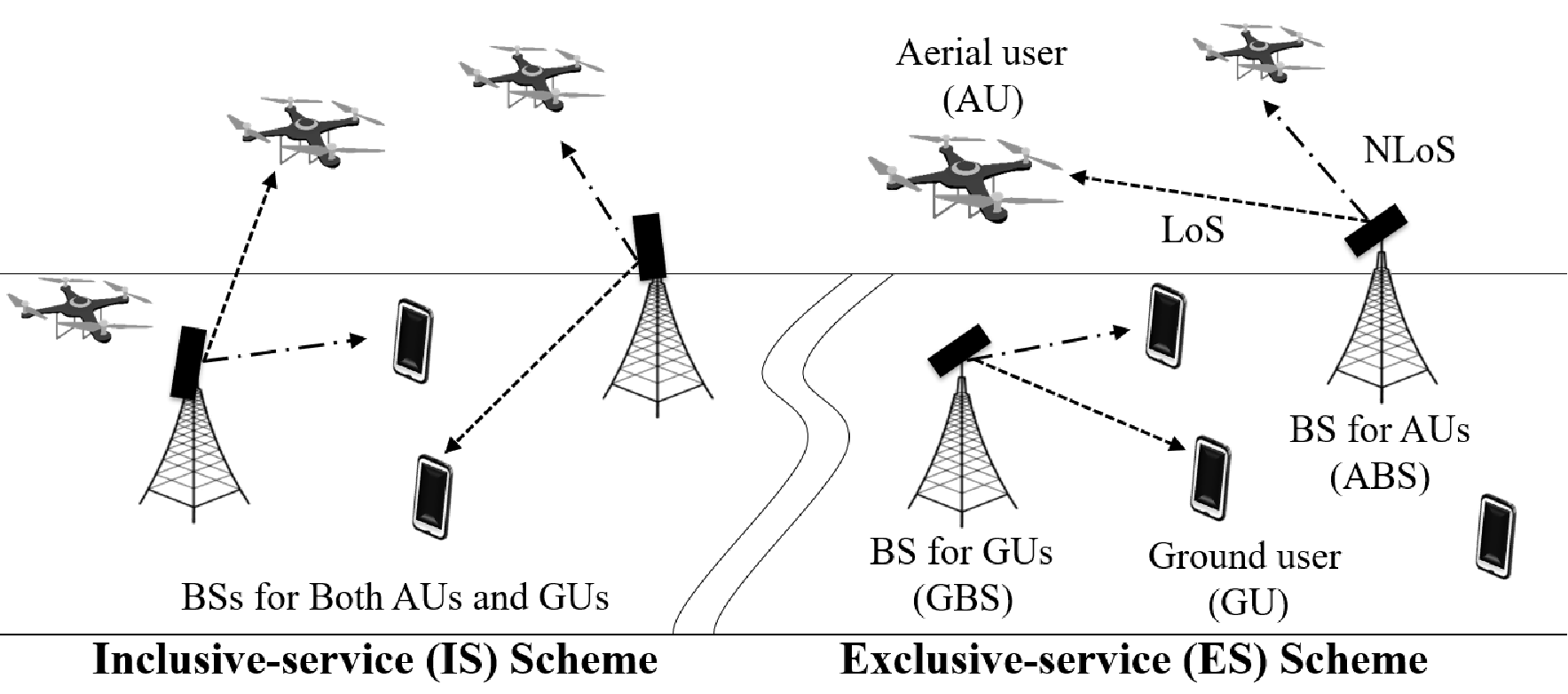
In this paper, as shown in Figure 1, we consider the two types of BS service provisioning schemes as follows.

• •

  Inclusive-service BS (IS-BS) scheme: In this scheme, BS serve both GU and AU simultaneously. Hence, the antenna tilt angle of the BS has to be designed to serve both GU and AU efficiently. The locations of BS are modeled by HPPP $\Phi_{\text{B},\text{O}}$ with density $\lambda_{\text{B}}$. Since there is only one type of BS, the BS density for GU, $\lambda^{\text{IS}}_{\text{B,G}}$, and the BS density for AU, $\lambda^{\text{IS}}_{\text{B,A}}$, are the same as the total BS density (i.e., $\lambda^{\text{IS}}_{\text{B,G}}=\lambda^{\text{IS}}_{\text{B,A}}=\lambda_{\text{B}}$). Note that this scheme is the one, generally used in prior works such as [22, 23, 25].

• •

  Exclusive-service BS (ES-BS) scheme: In this scheme, BS are divided into two groups: 1) a BS for GU ( GBS (GBS)) and 2) a BS for AU ( ABS (ABS)). The GBS and ABS exclusively serve GU and AU, respectively. Therefore, the antenna tilt angles of GBS and ABS need to be designed respectively to serve aimed users efficiently. We assume the distributions of GBS and ABS also follow HPPP, $\Phi_{\text{B},\text{G}}$ and $\Phi_{\text{B},\text{A}}$, with densities $\lambda^{\text{ES}}_{\text{B,G}}=\rho_{\text{B},\text{G}}\lambda_{\text{B}}$ and $\lambda^{\text{ES}}_{\text{B,A}}=(1-\rho_{\text{B},\text{G}})\lambda_{\text{B}}$, respectively, where $\rho_{\text{B},\text{G}}$ is the portion of GBS among all BS.

Regardless of BS types, for all BS, the antenna height is $h_{\text{B}}$ and the transmission power is $P_{\text{t}}$.

In UAV communications, both LoS and NLoS environments can be considered for the links between a BS and a GU as well as between a BS and an AU. The probability of forming LoS link between the BS at $\mathbf{x}=(x_{\text{B}},y_{\text{B}},h_{\text{B}})$ and the $k$th user at $(x_{k},y_{k},h_{k})$ is given by [32]²² 2 The LoS probability is also defined differently in [10]. However, it is determined by the elevation angle between the transmitter and the receiver, not by the link distance.

where $Q(x)\hskip-2.84526pt=\hskip-2.84526pt\int_{x}^{\infty}\!\frac{1}{\sqrt{2\pi}}\exp(-\frac{t^{2}}{2})\,dt$ is the Q-function and the horizontal distance between the BS and the $k$th user is given by $r_{k,\mathbf{x}}\hskip-2.84526pt=\hskip-2.84526pt\sqrt{\left(x_{k}\hskip-2.84526pt-\hskip-2.84526ptx_{\text{B}}\right)^{2}\hskip-2.84526pt+\hskip-2.84526pt\left(y_{k}-y_{\text{B}}\right)^{2}}$. Here, $\mu$, $\nu$ and $\xi$ are environment parameters determined by the density and the height of obstacles. Since the NLoS environment is a complementary event of the LoS environment, the NLoS probability between the BS and the $k$th user is given by $p_{\text{N}\hskip-1.70717pt}\left({r_{k,\mathbf{x}}}\right)=1-p_{\text{L}\hskip-1.70717pt}\left({r_{k,\mathbf{x}}}\right)$.

Based on the LoS probability, we consider different path loss exponents and channel fading models for LoS and NLoS links. The path loss exponent for LoS and NLoS links are denoted by $\alpha_{\text{L}}$ and $\alpha_{\text{N}}$, respectively. The channel fading is modeled by Nakagami-$m$ fading, so the distribution of the channel gain is given by

where $\Gamma(x)=\int_{0}^{\infty}t^{x-1}e^{-t}dt$ and $v\in\{\text{L},\text{N}\}$ is the channel environment, i.e., $v=\text{L}$ for LoS links and $v=\text{N}$ for NLoS links. In addition, we assume that $m_{\text{L}}>1$, and $m_{\text{N}}=1$, which means Rayleigh fading, i.e., $\Omega_{\text{N}}\sim\text{exp}(1)$. From (2), we denote the channel fading between the $k$th user and the BS as

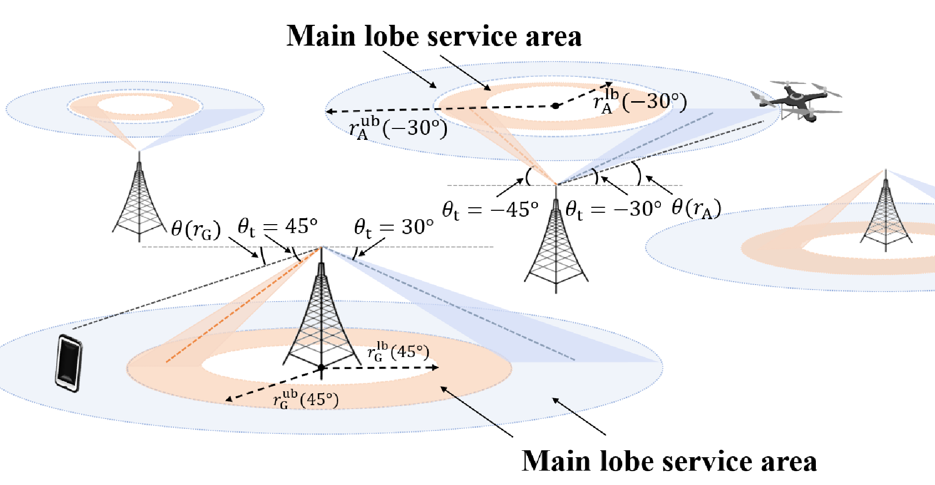
The antenna power gain of the BS is determined by two types of power gains: horizontal and vertical directional antenna gains. We consider an omnidirectional antenna in the horizontal direction, so the horizontal directional antenna gain remains constant regardless of the direction of the antenna. Therefore, we assume the horizontal directional antenna gain is equal to a unit gain [33]. In this paper, we focus on the design of the vertical antenna tilt angle for AU as well as GU, and we consider the directional antenna in the vertical direction. As shown in Fig. 2, the vertical directional antenna gain is determined by the vertical antenna tilt angle, $-90^{\circ}\hskip-1.42262pt<\hskip-1.42262pt\theta_{\text{t}}\hskip-1.42262pt<\hskip-1.42262pt90^{\circ}$, which is the angle tilted upward or downward relative to the horizontal plane.³³ 3 Note that there are two types of tilting methods[34]: mechanical tilting and electrical tilting. The mechanical tilting rotates the antenna of the BS physically. On the other hand, the electrical tilting applies an overall phase shift to all antenna elements in the array. In this paper, we consider the electrical tilting method to analyze the communication performance mathematically. Here, we define that the BS antenna tilt angle is a negative value when the BS antenna tilt angle is up-tilted, i.e., tilting upwards with respect to the horizontal plane of the BS antenna. On the other hand, the BS antenna tilt angle is defined as a positive value when the BS antenna tilt angle is down-tilted, i.e., tilting downwards with respect to the horizontal plane of the BS antenna. Based on the 3GPP (3GPP) specification [29], for given $r_{k,\mathbf{x}}$, the BS antenna power gain $G\hskip-0.85358pt(\hskip-0.85358ptr_{k,\mathbf{x}},\theta_{\text{t}}\hskip-0.85358pt)$ can be represented by a function of the tilt angle as

where $\theta_{\text{3dB}}=10^{\circ}$ is the 3dB beamwidth and $\eta$ is the minimum power leaking to the side lobe besides the main lobe, which is commonly 20dB. In (4), $\theta\left(r_{k,\mathbf{x}}\right)$ is the elevation angle between the BS antenna and the $k$th user, which is given by

where $h_{k}-h_{\text{B}}$ is the height difference between the BS and the $k$th user. In this work, without loss of generality, we assume that the height of AU is higher than that of BS (i.e., $h_{\text{A}}-h_{\text{B}}>0$), while the height of GU is lower than that of BS (i.e., $h_{\text{G}}-h_{\text{B}}<0$). From (4), for given $\theta_{\text{t}}$, the user can be served with the main lobe when $12\!\left(\!\frac{\theta\left(r_{k,\mathbf{x}}\right)+\theta_{\text{t}}}{\theta_{\text{3dB}}}\!\right)^{\!\!2}\geq\eta$. Here, we define the boundary of horizontal distance between a BS and the $k$th user that the user is served by the main lobe as $r_{k}^{\text{lb}}\left(\theta_{\text{t}}\right)\leq r_{k,\mathbf{x}}\leq r_{k}^{\text{ub}}\left(\theta_{\text{t}}\right)$, where $r_{k}^{\text{lb}}\left(\theta_{\text{t}}\right)$ and $r_{k}^{\text{ub}}\left(\theta_{\text{t}}\right)$ are the lower and upper boundaries. Since all GU and all AU have the same height, $h_{\text{G}}$ and $h_{\text{A}}$, respectively, the boundaries are determined by the user types not user’s specific location, i.e. $r_{k}^{\text{ub}}\left(\theta_{\text{t}}\right)=r_{i}^{\text{ub}}\left(\theta_{\text{t}}\right)$ and $r_{k}^{\text{lb}}\left(\theta_{\text{t}}\right)=r_{i}^{\text{lb}}\left(\theta_{\text{t}}\right)$ for $k\in\mathcal{U}_{i}$, and given as follows

where $\theta_{\text{th}}=\theta_{\text{3dB}}\sqrt{\eta/12}$. In (6)-(9), the boundaries $r_{i}^{\text{ub}}\left(\theta_{\text{t}}\right)$ and $r_{i}^{\text{lb}}\left(\theta_{\text{t}}\right)$ are defined to be positive when $\theta_{\text{t}}$ satisfies each conditions. For the convenience of analysis, we rewrite $G\left(r_{k,\mathbf{x}},\theta_{\text{t}}\right)$ in (4) according to the boundaries in (6)-(9) as

where $b_{k,{1}}(\theta_{\text{t}})=0,b_{k,{2}}(\theta_{\text{t}})=r_{k}^{\text{lb}}\left(\theta_{\text{t}}\right),b_{k,{3}}(\theta_{\text{t}})=r_{k}^{\text{ub}}\left(\theta_{\text{t}}\right)$, and $b_{k,{4}}(\theta_{\text{t}})=\infty$. In (10), $G_{1}(r_{k,\mathbf{x}},\theta_{\text{t}})=G_{3}(r_{k,\mathbf{x}},\theta_{\text{t}})=10^{-\eta/10}$ is the antenna side lobe gain and $G_{2}(r_{k,\mathbf{x}},\theta_{\text{t}})$ is the antenna main lobe gain, which is given by

From (11), we can see that $G_{2}(r_{k,\mathbf{x}},\theta_{\text{t}})$ is an increasing function of $\theta_{\text{t}}$ for $-\theta_{\text{th}}<\theta_{\text{t}}\leq-\theta\left(r_{k,\mathbf{x}}\right)$, and $G_{2}(r_{k,\mathbf{x}},\theta_{\text{t}})$ is a decreasing function of $\theta_{\text{t}}$ for $-\theta\left(r_{k,\mathbf{x}}\right)\leq\theta_{\text{t}}<\theta_{\text{th}}$. This is because as the antenna tilt angle $\theta_{\text{t}}$ approaches the elevation angle between the BS and the user, the effect of the main lobe becomes dominant and it is maximized when the antenna tilt angle is equal to the elevation angle (i.e., $\theta_{\text{t}}=-\theta\left(r_{k,\mathbf{x}}\right)$).

In conventional networks, the BS association is determined by the mean channel fading gain and the distance-dependent path loss, considering the LoS probability [35]. However, in more realistic UAV networks, the antenna gain $G\left(r_{k,\mathbf{x}},\theta_{\text{t}}\right)$ affected by the horizontal distance between the serving BS and the $k$th user should also be considered in the BS association.

To analyze BS association rules, we first denote BS which belong to $\Phi_{\text{B},l},l\in{\text{\lx@text@lbrace O,G,A\lx@text@rbrace}}$, forming LoS and NLoS links as $\Phi^{\text{L}}_{\text{B},l}$ and $\Phi^{\text{N}}_{\text{B},l}$, respectively. We then divide each of $\Phi^{\text{L}}_{\text{B},l}$ and $\Phi^{\text{N}}_{\text{B},l}$ into three groups according to the BS antenna power gain $G\left(r_{k,\mathbf{x}},\theta_{\text{t}}\right)$ in (10) as

where $j\hskip-2.84526pt\in\hskip-2.84526pt\mathcal{J}$ is the index of BS groups which is determined by $r_{k,\mathbf{x}}$, and $\mathcal{J}\hskip-4.2679pt=\hskip-4.2679pt\{\hskip-1.42262pt1,2,3\hskip-1.42262pt\}$. Note that from (10) and (12), we know that BS in $\Phi^{v1}_{\text{B},l}$ or $\Phi^{v3}_{\text{B},l}$ transmit with the antenna side lobe gain, and BS in $\Phi^{v2}_{\text{B},l}$ transmit with the antenna main lobe gain. First of all, we examine the distribution of the distance between the user and the BS in $\Phi^{vj}_{\text{B},l}$ . The horizontal distance to the nearest BS among the BS in $\Phi^{vj}_{\text{B},l}$ is denoted by $X_{k}^{vj}$. Here, depending on the LoS probability, the density function of $\Phi^{vj}_{\text{B},l}$ is given by $2\pi\lambda_{\text{B},k}^{s}tp_{v}(t)$. Therefore, for BS in $\Phi^{vj}_{\text{B},l}$, the CCDF (CCDF) of $X_{k}^{vj}$ can be obtained as

where (a) is from the void probability[36] and $u_{k,j}(x,\theta_{\text{t}})$ is given as $u_{k,1}(x,\theta_{\text{t}})=\text{min}(x,b_{k,{j+1}}(\theta_{\text{t}}))$ if $j=1$, $u_{k,j}(x,\theta_{\text{t}})=\text{max}(x,b_{k,{j}}(\theta_{\text{t}}))$, otherwise. $\lambda_{\text{B},k}^{s}$ is the density of BS that can serve the $k$th user, i.e., $\lambda_{\text{B},k}^{s}=\lambda_{\text{B},i}^{s}$ when $k\in\mathcal{U}_{i}$. Here, $s\in\left\{\text{IS},\text{ES}\right\}$ is the index of the BS service provisioning scheme. By differentiating (13), we can obtain the PDF (PDF) of $X_{k}^{vj}$ as

where $f^{s}_{X_{k}^{vj}}(x)=0$ if $x\leq b_{k,{j}}(\theta_{\text{t}})$.

We denote $a\in\{{\text{na},\text{sa}}\}$ as the index of the BS association criterion. Here, $a=\text{na}$ and $a=\text{sa}$ indicate the nearest BS association rule and the strongest BS association rule, respectively.

We assume that the available frequency resource is divided into $N$ sub-bands, and the interfering BS are the ones that use the same sub-band. Hence, in the IS-BS scheme, the distribution of the interfering BS is modeled as a HPPP $\Phi_{\text{I},\text{O}}$ with density $\lambda^{\text{IS}}_{\text{I},\text{O}}=\lambda_{\text{B}}/N$ such as in [37]. In the ES-BS scheme, the interference from GBS and ABS needs to be defined differently as they use different tilt angles. The distributions of interfering GBS and ABS are also modeled as HPPP, $\Phi_{\text{I},\text{G}}$ and $\Phi_{\text{I},\text{A}}$, with densities $\lambda^{\text{ES}}_{\text{I},\text{G}}=\lambda^{\text{ES}}_{\text{B,G}}/N$ and $\lambda^{\text{ES}}_{\text{I},\text{A}}=\lambda^{\text{ES}}_{\text{B,A}}/N$, respectively.

For the case that a BS communicates with the $k$th user, the SINR at the user can be given by

where $l_{v\hskip-1.42262pt}\left(r_{k,\mathbf{x}_{\tau}}\right)\hskip-2.27621pt=\hskip-2.27621pt\left(\hskip-1.42262ptr_{k,\mathbf{x}}^{2}\hskip-1.42262pt+\hskip-1.42262pt\left(h_{k}\hskip-2.84526pt-\hskip-2.84526pth_{\text{B}}\right)^{2}\right)^{\hskip-2.84526pt-\frac{\alpha_{v}}{2}},v\in\{\text{L},\text{N}\}$, is the distance-dependent path loss between the $k$th user and the BS at $\mathbf{x}$ for LoS and NLoS links, and $\sigma^{2}$ is the noise power.

In (20), $I^{\text{IS}}\hskip-1.42262pt=\hskip-1.42262ptI^{\text{IS}}_{\text{O}}$ and $I^{\text{ES}}\hskip-1.42262pt=\hskip-1.42262ptI^{\text{ES}}_{\text{G}}+I^{\text{IS}}_{\text{A}}$, where $I^{s}_{l}$ is given by

Using the SINR in (20), when the user associates to a $j$-group BS with the distance $r_{k,\mathbf{x}_{\tau}}$ and the tilt angle $\theta_{\text{t}}$ under the channel environment $v$, the outage probability is given by

where $\gamma_{\text{t}}=2^{\frac{R_{\text{o}}}{W}}-1$ is the target SINR. Here, $R_{\text{o}}$ is the target data rate and $W$ is the bandwidth allocated to each user [38]. In the following theorem, we derive the network outage probability. For readability, instead of notation $\theta_{\text{t}}$, when scheme $s$ is used, we denote antenna tilt angles of the GBS and the ABS as $\theta^{s}_{\text{t,G}}$ and $\theta^{s}_{\text{t,A}}$, respectively. Note that in the IS-BS scheme, since all BS serve both GU and AU, we have a single antenna tilt angle $\theta^{\text{IS}}_{\text{t,O}}$, i.e., $\theta^{\text{IS}}_{\text{t,G}}=\theta^{\text{IS}}_{\text{t,A}}=\theta^{\text{IS}}_{\text{t,O}}$.

References

- [1] S. Kim, M. Kim, J. Y. Ryu, and J. lee, “Impact of base station antenna tilt angle on UAV communications,” in Proc. IEEE Global Commun. Conf. (GLOBECOM), Taipei, Taiwan, Dec. 2020, pp. 1–6.
- [2] F. Rinaldi, H.-L. Maattanen, J. Torsner, S. Pizzi, S. Andreev, A. Iera, Y. Koucheryavy, and G. Araniti, “Non-terrestrial networks in 5G & beyond: A survey,” IEEE Access, vol. 8, pp. 165 178–165 200, Sep. 2020.
- [3] M. Giordani and M. Zorzi, “Non-terrestrial networks in the 6G era: Challenges and opportunities,” IEEE Netw., vol. 35, no. 2, pp. 244–251, Mar. 2021.
- [4] X. Lin, S. Rommer, S. Euler, E. A. Yavuz, and R. S. Karlsson, “5G from space: An overview of 3GPP non-terrestrial networks,” arXiv, Mar. 2021. [Online]. Available: https://arxiv.org/abs/2103.09156
- [5] Y. Zeng, R. Zhang, and T. J. Lim, “Wireless communications with unmanned aerial vehicles: opportunities and challenges,” IEEE Commun. Mag., vol. 54, no. 5, pp. 36–42, May 2016.
- [6] N. H. Motlagh, M. Bagaa, and T. Taleb, “UAV-based IoT platform: A crowd surveillance use case,” IEEE Commun. Mag., vol. 55, no. 2, pp. 128–134, Feb. 2017.
- [7] S. Hayat, E. Yanmaz, and R. Muzaffar, “Survey on unmanned aerial vehicle networks for civil application: A communications viewpoint,” IEEE Commun. Surveys Tuts., vol. 18, no. 4, pp. 2624–2661, Fourth Quart. 2016.
- [8] A. A. Khuwaja, Y. Chen, N. Zhao, M. Alouini, and P. Dobbins, “A survey of channel modeling for UAV communications,” IEEE Commun. Surveys Tuts., vol. 20, no. 4, pp. 2804–2821, Fourth Quart. 2018.
- [9] A. Al-Hourani and K. Gomez, “Modeling cellular-to-UAV path-loss for suburban environments,” IEEE Wireless Commun. Lett., vol. 7, no. 1, pp. 82–85, Feb. 2018.
- [10] A. Al-Hourani, S. Kandeepan, and S. Lardner, “Optimal LAP altitude for maximum coverage,” IEEE Wireless Commun. Lett., vol. 3, no. 6, pp. 569–572, Dec. 2014.
- [11] H. Cho, C. Liu, J. Lee, T. Noh, and T. Q. S. Quek, “Impact of elevated base stations on the ultra-dense networks,” IEEE Commun. Lett., vol. 22, no. 6, pp. 1268–1271, Jun. 2018.
- [12] M. M. Azari, F. Rosas, K. Chen, and S. Pollin, “Ultra reliable UAV communication using altitude and cooperation diversity,” IEEE Trans. Commun., vol. 66, no. 1, pp. 330–344, Jan. 2018.
- [13] P. K. Sharma and D. I. Kim, “UAV-enabled downlink wireless system with non-orthogonal multiple access,” in Proc. IEEE Global Commun. Conf. Workshops. (GC Wkshps), Singapore, Dec. 2017, pp. 1–6.
- [14] H. He, S. Zhang, Y. Zeng, and R. Zhang, “Joint altitude and beamwidth optimization for UAV-enabled multiuser communications,” IEEE Commun. Lett., vol. 22, no. 2, pp. 344–347, Feb. 2018.
- [15] M. Mozaffari, W. Saad, M. Bennis, and M. Debbah, “Efficient deployment of multiple unmanned aerial vehicles for optimal wireless coverage,” IEEE Commun. Lett., vol. 20, no. 8, pp. 1647–1650, Aug. 2016.
- [16] J. Lyu, Y. Zeng, and R. Zhang, “UAV-aided offloading for cellular hotspot,” IEEE Trans. Wireless Commun., vol. 17, no. 6, pp. 3988–4001, Jun. 2018.
- [17] S. Zhang, Y. Zeng, and R. Zhang, “Cellular-enabled UAV communication: A connectivity-constrained trajectory optimization perspective,” IEEE Trans. Commun., vol. 67, no. 3, pp. 2580–2604, Mar. 2019.
- [18] M. Kim and J. Lee, “Impact of an interfering node on unmanned aerial vehicle communications,” IEEE Trans. Veh. Technol., vol. 68, no. 12, pp. 12 150–12 163, Dec. 2019.
- [19] D. Kim, J. Lee, and T. Q. S. Quek, “Multi-layer unmanned aerial vehicle networks: Modeling and performance analysis,” IEEE Trans. Wireless Commun., vol. 19, no. 1, pp. 325–339, Jan. 2020.
- [20] Y. Zeng, J. Lyu, and R. Zhang, “Cellular-connected UAV: Potential, challenges, and promising technologies,” IEEE Wireless Commun., vol. 26, no. 1, pp. 120–127, Feb. 2019.
- [21] X. Lin, V. Yajnanarayana, S. D. Muruganathan, S. Gao, H. Asplund, H. Maattanen, M. Bergstrom, S. Euler, and Y. . E. Wang, “The sky is not the limit: LTE for unmanned aerial vehicles,” IEEE Commun. Mag., vol. 56, no. 4, pp. 204–210, Apr. 2018.
- [22] B. Galkin, J. Kibilda, and L. A. DaSilva, “Backhaul for low-altitude UAVs in urban environments,” in Proc. IEEE Int. Conf. Commun. (ICC), Kansas City, MO, May 2018, pp. 1–6.
- [23] M. M. Azari, F. Rosas, A. Chiumento, and S. Pollin, “Coexistence of terrestrial and aerial users in cellular networks,” in Proc. IEEE Global Commun. Conf. Workshops. (GC Wkshps), Singapore, Dec. 2017, pp. 1–6.
- [24] M. M. Azari, F. Rosas, and S. Pollin, “Reshaping cellular networks for the sky: Major factors and feasibility,” in Proc. IEEE Int. Conf. Commun. (ICC), Kansas City, MO, May 2018, pp. 1–7.
- [25] R. Amer, W. Saad, and N. Marchetti, “Toward a connected sky: Performance of beamforming with down-tilted antennas for ground and UAV user co-existence,” IEEE Commun. Lett., vol. 23, no. 10, pp. 1840–1844, Oct. 2019.
- [26] X. Xu and Y. Zeng, “Cellular-connected UAV: Performance analysis with 3D antenna modeling,” in Proc. IEEE Int. Conf. Commun. Workshops. (ICC Wkshps), Shanghai, China, May 2019, pp. 1–6.
- [27] R. Amer, W. Saad, B. Galkin, and N. Marchetti, “Performance analysis of mobile cellular-connected drones under practical antenna configurations,” in Proc. IEEE Int. Conf. Commun. (ICC), Dublin, Ireland, Jun. 2020, pp. 1–7.
- [28] R. Amer, W. Saad, and N. Marchetti, “Mobility in the sky: Performance and mobility analysis for cellular-connected UAVs,” IEEE Trans. Commun., vol. 68, no. 5, pp. 3229–3246, May 2020.
- [29] 3rd Generation Partnership Project, “Technical specification group radio access network; evolved universal terrestrial radio access (E-UTRA); further advancements for E-UTRA physical layer aspects,” TR 36.814 V9.2.0, Tech. Rep., Mar. 2017, release 9.
- [30] Y. Zhu, G. Zheng, and M. Fitch, “Secrecy rate analysis of uav-enabled mmwave networks using matérn hardcore point processes,” IEEE J. Sel. Areas Commun., vol. 36, no. 7, pp. 1397–1409, Jul. 2018.
- [31] J. Lyu and H.-M. Wang, “Secure uav random networks with minimum safety distance,” IEEE Trans. Veh. Technol., vol. 70, no. 3, pp. 2856–2861, Mar. 2021.
- [32] Z. Yang, L. Zhou, G. Zhao, and S. Zhou, “Blockage modeling for inter-layer UAVs communications in urban environments,” in Proc. IEEE Int. Conf. Telecommun. (ICT), St. Malo, France, Jun. 2018, pp. 307–311.
- [33] R. Hernandez-Aquino, S. A. R. Zaidi, D. McLernon, M. Ghogho, and A. Imran, “Tilt angle optimization in two-tier cellular networks—a stochastic geometry approach,” IEEE Trans. Commun., vol. 63, no. 12, pp. 5162–5177, Dec. 2015.
- [34] S. M. Razavizadeh, M. Ahn, and I. Lee, “Three-dimensional beamforming: A new enabling technology for 5g wireless networks,” IEEE Signal Process. Mag., vol. 31, no. 6, pp. 94–101, Nov. 2014.
- [35] M. Alzenad and H. Yanikomeroglu, “Coverage and rate analysis for unmanned aerial vehicle base stations with LoS/NLoS propagation,” in Proc. IEEE Global Commun. Conf. Workshops. (GC Wkshps), Abu Dhabi, UAE, Dec. 2018, pp. 1–7.
- [36] F. Baccelli and B. Błaszczyszyn, Stochastic Geometry and Wireless Networks, Volume II — Applications, ser. Foundations and Trends in Networking. NoW Publishers, 2009.
- [37] H. ElSawy, A. Sultan-Salem, M. Alouini, and M. Z. Win, “Modeling and analysis of cellular networks using stochastic geometry: A tutorial,” IEEE Commun. Surveys Tuts., vol. 19, no. 1, pp. 167–203, First Quart. 2017.
- [38] S. S. Ikki and M. H. Ahmed, “Performance analysis of decode-and-forward incremental relaying cooperative-diversity networks over rayleigh fading channels,” in Proc. IEEE Veh. Technol. Conf. (VTC), Barcelona, Spain, Apr. 2009, pp. 1–6.
- [39] I. S. Gradshteyn and I. M. Ryzhik, Table of Integrals, Series, and Products, 7th ed. San Diego, CA, USA: Academic Press, 2007.
- [40] 3rd Generation Partnership Project, “Technical specification group radio access network; study on enhanced lte support for aerial vehicles,” TR 36.777 V15.0.0, Tech. Rep., Dec. 2017, release 15.
- [41] J. Holis and P. Pechac, “Elevation dependent shadowing model for mobile communications via high altitude platforms in built-up areas,” IEEE Trans. Antennas Propag., vol. 56, no. 4, pp. 1078–1084, Apr. 2008.
- [42] M. Haenggi and R. K. Ganti, “Interference in large wireless networks,” Foundations and Trends in Networking, vol. 3, no. 2, pp. 127–248, 2009.