TAAC: Temporally Abstract Actor-Critic for Continuous Control
Abstract
We present temporally abstract actor-critic (TAAC), a simple but effective off-policy RL algorithm that incorporates closed-loop temporal abstraction into the actor-critic framework. TAAC adds a second-stage binary policy to choose between the previous action and a new action output by an actor. Crucially, its “act-or-repeat” decision hinges on the actually sampled action instead of the expected behavior of the actor. This post-acting switching scheme let the overall policy make more informed decisions. TAAC has two important features: a) persistent exploration, and b) a new compare-through Q operator for multi-step TD backup, specially tailored to the action repetition scenario. We demonstrate TAAC’s advantages over several strong baselines across 14 continuous control tasks. Our surprising finding reveals that while achieving top performance, TAAC is able to “mine” a significant number of repeated actions with the trained policy even on continuous tasks whose problem structures on the surface seem to repel action repetition. This suggests that aside from encouraging persistent exploration, action repetition can find its place in a good policy behavior. Code will be made public.
1 Introduction
Deep reinforcement learning (RL) has achieved great success in various continuous action domains such as locomotion and manipulation (Schulman et al., 2015; Lillicrap et al., 2016; Duan et al., 2016; Schulman et al., 2017; Fujimoto et al., 2018; Haarnoja et al., 2018). Despite promising empirical results, these widely applicable continuous RL algorithms execute a newly computed action at every step of the finest time scale of a problem. With no decision making at higher levels, they attempt to solve the challenging credit assignment problem over a long horizon. As a result, considerable sample efficiency improvements have yet to be made by them in complex task structures (Riedmiller et al., 2018; Li et al., 2020; Lee et al., 2020b) and extremely sparse reward settings (Andrychowicz et al., 2017; Plappert et al., 2018; Zhang et al., 2021).
On the other hand, it is argued that temporal abstraction (Parr and Russell, 1998; Dietterich, 1998; Sutton et al., 1999; Precup, 2000) is one of the crucial keys to solving control problems with complex structures. Larger steps are taken at higher levels of abstraction while lower-level actions only need to focus on solving isolated subtasks (Dayan and Hinton, 1993; Vezhnevets et al., 2017; Bacon et al., 2017). However, most hierarchical RL (HRL) methods are task specific and nontrivial to adapt. For example, the options framework (Sutton et al., 1999; Precup, 2000; Bacon et al., 2017) requires pre-defining an option space, while the feudal RL framework Vezhnevets et al., 2017; Nachum et al., 2018; Zhang et al., 2021 requires tuning the hyperparameters of dimensionality and domain range of the goal space. In practice, their final performance usually hinges on these choices.
Perhaps the simplest form of an option or sub-policy would be just repeating an action for a certain number of steps, a straightforward idea that has been widely explored (Lakshminarayanan et al., 2017; Sharma et al., 2017; Dabney et al., 2021; Metelli et al., 2020; Lee et al., 2020a; Biedenkapp et al., 2021). This line of works can be regarded as a middle ground between “flat” RL and HRL. They assume a fixed candidate set of action durations, and repeat actions in an open-loop manner. Open-loop control forces an agent to commit to the same action over a predicted duration with no opportunity of early terminations. It weakens the agent’s ability of handling emergency situations and correcting wrong durations predicted earlier. To address this inflexibility, a handful of prior works (Neunert et al., 2020; Chen et al., 2021) propose to output an “act-or-repeat” binary decision to decide if the action at the previous step should be repeated. Because this “act-or-repeat” decision will be examined at every step depending on the current environment state, this results in closed-loop action repetition.
All these action-repetition methods are well justified by the need of action persistence (Dabney et al., 2021; Amin et al., 2021; Zhang and Van Hoof, 2021; Grigsby et al., 2021) for designing a good exploration strategy, when action diversity should be traded for it properly. This trade-off is important because when reward is sparse or short-term reward is deceptive, action diversity alone only makes the agent wandering around its local neighborhood since any persistent trajectory has an exponentially small probability. In such a case, a sub-optimal solution is likely to be found. In contrast, persistence via action repetition makes the policy explore deeper (while sacrificing action diversity to some extent).
This paper further explores in the direction of closed-loop action repetition, striving to discover a novel algorithm that instantiates this idea better. The key question we ask is, how can we exploit the special structure of closed-loop repetition, so that our algorithm yields better sample efficiency and final performance compared to existing methods? As an answer to this question, we propose temporally abstract actor-critic (TAAC), a simple but effective off-policy RL algorithm that incorporates closed-loop action repetition into an actor-critic framework. Generally, we add a second stage that chooses between a candidate action output by an actor and the action from the previous step (Figure 1). Crucially, its “act-or-repeat” decision hinges on the actually sampled individual action instead of the expected behavior of the actor unlike recent works (Neunert et al., 2020; Chen et al., 2021). This post-acting switching scheme let the overall policy make more informed decisions. Moreover,
- i)
for policy evaluation, we propose a new compare-through Q operator for multi-step TD backup tailored to the action repetition scenario, instead of replying on generic importance correction;
- ii)
for policy improvement, we compute the actor gradient by multiplying a scaling factor to the term from DDPG (Lillicrap et al., 2016) and SAC (Haarnoja et al., 2018), where the scaling factor is the optimal probability of choosing the actor’s action in the second stage.
TAAC is much easier to train compared to sophisticated HRL methods, while it has two important features compared to “flat” RL algorithms, namely, persistent exploration and native multi-step TD backup support without the need of off-policyness correction.
We evaluate TAAC on 14 continuous control tasks, covering simple control, locomotion, terrain walking (Brockman et al., 2016), manipulation (Plappert et al., 2018), and self-driving (Dosovitskiy et al., 2017). Averaged over these tasks, TAAC largely outperforms 6 strong baselines. Importantly, our results show that it is our concrete instantiation of closed-loop action repetition that is vital to the final performance. The mere idea of repeating actions in a closed-loop manner doesn’t guarantee better results than the compared open-loop methods. Moreover, our surprising finding reveals that while achieving top performance, TAAC is able to “mine” a significant number of repeated actions with the trained policy even on continuous tasks whose problem structures on the surface seem to repel action repetition (Section 5.6.2). This suggests that aside from encouraging persistent exploration, action repetition can find its place in a good policy behavior. This is perhaps due to that the action frequency of a task can be difficult to be set exactly as the minimum value that doesn’t comprise optimal control while leaving no room for temporal abstraction (Grigsby et al., 2021).
2 Related work
Under the category of temporal abstraction via action repetition, there have been various formulations. Dabney et al., 2021 proposes temporally extended -greedy exploration where a duration for repeating actions is sampled from a pre-defined truncated zeta distribution. This strategy only affects the exploration behavior for generating off-policy data but does not change the training objective. Sharma et al., 2017 and Biedenkapp et al., 2021 learn a hybrid action space and treat the discrete action as a latent variable of action repeating steps, but the introduced temporal abstraction is open-loop and lacks flexibility. One recent work close to TAAC is PIC (Chen et al., 2021) which also learns to repeat the last action to address the action oscillation issue within consecutive steps. However, PIC was proposed for discrete control and its extension to continuous control is unclear yet. Also, PIC predicts whether to repeat the last action independent of a newly sampled action, which requires its switching policy to make a decision regarding the core policy’s expected behavior. In an application section, H-MPO (Neunert et al., 2020) explored how continuous control can benefit from a meta binary action that modifies the overall system behavior. Again, like PIC their binary decision is made in parallel with a newly sampled action. Different from PIC and H-MPO, TAAC only decides “act-or-repeat” after comparing the previous action with a newly sampled action. Moreover, TAAC employs a new compare-through Q operator to exploit repeated actions for multi-step TD backup, and is trained by a much simpler actor gradient by absorbing the closed-form solution of the binary policy into the continuous action objective to avoid parameterizing a discrete policy unlike H-MPO.
3 Preliminaries
We consider the RL problem as policy search in a Markov Decision Process (MDP). Let denote a state, where a continuous action is taken. Let be the action policy, and the probability of the environment transitioning to after an action is taken at . Upon reaching , the agent receives a scalar reward . The RL objective is to find a policy that maximizes the expected discounted return: , where is a discount factor. We also define as the discounted return starting from given that is taken and then is followed, and as the discounted return starting from following .
In an off-policy actor-critic setting with and parameterized by and , a surrogate objective is usually used (Lillicrap et al., 2016; Haarnoja et al., 2018)
| (1) |
This objective maximizes the expected state value over some state distribution, assuming that 1) is sampled from a replay buffer instead of the current policy, and 2) the dependency of the critic on the policy is dropped when computing the gradient of . Meanwhile, is learned separately via policy evaluation with typical TD backup.
4 Temporally abstract actor-critic

To enable temporal abstraction, we decompose the agent’s action decision into two stages (Figure 1): 1) sampling a new candidate action conditioned on the action at the previous time step, and 2) choosing between and as the actual output at the current step. The overall TAAC algorithm is summarized in Algorithm 1 Appendix A.
4.1 Two-stage policy
Formally, let be the binary switching policy, where / means choosing /. For simplicity, in the following we will denote (always assuming its dependency on , , and ). Then our two-stage policy for temporal abstraction is defined as
| (2) |
which can be shown to be a proper probability distribution of . This two-stage policy repeats previous actions through a binary policy , a decision maker that compares and side by side given the current state . Repeatedly favoring results in temporal abstraction of executing the same action for multiple steps. Moreover, this control is closed-loop, as it does not commit to a pre-determined time window; instead it can stop repetition whenever necessary. As a special case, when , reduces to ; when , .
4.2 Policy evaluation with the compare-through operator
The typical one-step TD learning objective for a policy is
| (3) |
where is the Bellman operator, and slowly tracks to stabilize the learning (Mnih et al., 2015). For multi-step bootstrapping, importance correction is usually needed, for example, Retrace (Munos et al., 2016) relies on a function of ( is a behavior policy) to correct for the off-policyness of a trajectory. Unfortunately, our makes probability density computation challenging because of the marginalization over . Thus importance correction methods including Retrace cannot be applied to our case. To address this issue, below we propose a new multi-step Q operator, called compare-through. Then we explain how can exploit this operator for efficient policy evaluation.
For a learning policy , given a trajectory from a behavior policy , let denote the actions sampled from at states and (we do not sample from at ). We define (a point estimate of) the compare-through operator as
| (4) |
where . Intuitively, given a sampled trajectory of length from the replay buffer, the compare-through operator takes an expectation, under the current policy at the sampled states (from to ), over all the sub-trajectoriess (up to length ) of actions that match the sampled actions. Note that Eq. 4 is a point estimate of this expectation. A formal definition of is described by Eq. 17, and its relation to Retrace (Munos et al., 2016) is shown in Appendix L.

Theorem 1 (Policy evaluation convergence)
For the detailed proof we refer the reader to Appendix L. Although the actual setting considered in this paper are continuous state and action domains with function approximators, Theorem 1 still provides some justification for our compare-through operator.
Clearly, any discrete policy could exploit the compare-through operator since there can be a non-zero chance of two discrete actions being compared equal. A typical stochastic continuous policy such as Gaussian used by SAC (Haarnoja et al., 2018) always has for w.r.t. any behavior policy . In this case is no more than just a Bellman operator . However, if a continuous policy is specially structured to be “action-reproducible”, it will enjoy the privilege of using for as the target state. Our two-stage is such a case, where each action () is accompanied by a repeating choice (). Starting from with a previous action , if (both repeated) for all , then we know that . In other words, if two trajectories start with the same , we can compare their discrete sequences in place of the continuous sequences. See Figure 2 for an illustration. Thus for multi-step TD learning we use to replace in Eq. 3.
Remark The compare-through operator is not meant to replace multi-step TD learning with importance correction in a general scenario, as it is only effective for “action-reproducible” policies. Its bootstrapping has a hard cutoff (by checking ) instead of a soft one as in Munos et al., 2016.
On the importance of reward normalization Because computes bootstrapping targets based on dynamic step lengths and rewards are propagated faster with greater lengths, Q values bootstrapped by greater lengths might become overly optimistic/pessimistic (e.g., imagine a task with rewards that are all positive/negative). This could affect the policy selecting actions according to their Q values. However, this side effect is only temporary and will vanish if all Q values are well learned eventually. In practice, we find it beneficial to normalize the immediate reward by its moving average statistics to roughly maintain a zero mean and unit standard deviation (detailed in Appendix I.1).
4.3 Policy improvement with a closed-form
It can be shown (Appendix B) that the parameterized state value of is
| (5) |
Intuitively, the actual Q value of each is an interpolation by between the Q values of and . Our policy improvement objective is then . Note that each time we sample the previous action along with a state from the replay buffer. To encourage exploration, following prior works (Mnih et al., 2016; Riedmiller et al., 2018) we augment this objective with a joint entropy . Thus the final policy improvement objective is
| (6) |
where is a temperature parameter. Given any , we can derive a closed-form solution of the (non-parametric) policy for the innermost expectation as
Then applying the re-parameterization trick , one can show that the estimated actor gradient is
| (7) |
This gradient has a very similar form with SAC’s (Haarnoja et al., 2018), except that here has a scaling factor . We refer the reader to a full derivation of the actor gradient in Appendix D.
Remark on This closed-form solution is only possible after is sampled. It’s essentially comparing the Q values between and . This side-by-side comparison is absent in previous closed-loop repeating methods like PIC (Chen et al., 2021) and H-MPO (Neunert et al., 2020).
Remark on multi-step actor gradient According to Figure 1, the newly generated action at the current step , if repeated as future (), will also influence the maximization of future V values: . As a result, in principle has a multi-step gradient. To exactly compute this multi-step gradient, a fresh rollout of the current via interacting with the environment is necessary. For reasons detailed in Appendix E, we end up truncating this full gradient to the first step, by letting Eq. 6 sample pairs at non-consecutive time steps from the replay buffer. This one-step truncation is also (implicitly) adopted by H-MPO (Neunert et al., 2020) for their action repetition application case. Interestingly, the truncation results in a simple implementation of actor gradient of TAAC similar to SAC’s.
Automatically tuned temperatures Given two entropy targets and , we learn temperatures and from the objective
| (8) |
by adjusting instead of as in SAC (Haarnoja et al., 2018). We learn temperatures for and separately, to enable a finer control of the two policies and their entropy terms, similar to the separate policy constraints (Abdolmaleki et al., 2018; Neunert et al., 2020). Appendix F shows how several equations slightly change if two temperatures are used ( is replaced by or ).
5 Experiments
5.1 Tasks
To test if the proposed algorithm is robust and can be readily applied to many tasks, we perform experiments over 14 continuous control tasks under different scenarios:
- a)
SimpleControl: Three control tasks (Brockman et al., 2016) with small action and observation spaces: MountainCarContinuous, LunarLanderContinuous, and InvertedDoublePendulum ;
- b)
Locomotion: Four locomotion tasks (Brockman et al., 2016) that feature complex physics and action spaces: Hopper, Ant, Walker2d, and HalfCheetah;
- c)
Terrain: Two locomotion tasks that require adapting to randomly generated terrains: BipedalWalker and BipedalWalkerHardcore;
- d)
Manipulation: Four Fetch (Plappert et al., 2018) tasks with sparse rewards and hard exploration (reward given only upon success): FetchReach, FetchPush, FetchSlide, and FetchPickAndPlace;
- e)
Driving: One CARLA autonomous-driving task (Dosovitskiy et al., 2017) that has complex high-dimensional multi-modal sensor inputs (camera, radar, IMU, collision, GPS, etc.): Town01. The goal is to reach a destination starting from a randomly spawned location in a small realistic town, while avoiding collisions and red light violations.
Among the 5 categories, (d) and (e) might benefit greatly from temporal abstraction because of hard exploration or the problem structure (e.g., driving naturally involves repeated actions). Categories (a)-(c) appear unrelated with temporal abstraction, but we test if seemingly unrelated tasks can also benefit from it. By comparing TAAC against different methods across vastly different tasks, we hope to demonstrate its generality, because adaptation to this kind of task variety requires few assumptions about the task structure and inputs/outputs. For more task details, we refer the reader to Appendix I.
| SAC | SAC-Ntd | SAC-Nrep | SAC-Krep | SAC-EZ | SAC-Hybrid | TAAC-1td | TAAC | |
| (Haarnoja et al., 2018) | (Sharma et al., 2017) | (Dabney et al., 2021) | (Neunert et al., 2020) | |||||
| (Biedenkapp et al., 2021) | ||||||||
| Persistent exploration | ✗ | ✗ | ✓ | ✓ | ✓ | ✓ | ✓ | ✓ |
| Multi-step TD | ✗ | ✓ | ✓ | ✓ | ✗ | ✓ | ✗ | ✓ |
| Closed-loop repetition | ✗ | ✗ | ✗ | ✗ | ✗ | ✓ | ✓ | ✓ |
| Learnable duration | ✗ | ✗ | ✗ | ✓ | ✗ | ✓ | ✓ | ✓ |
5.2 Comparison methods
While there exist many off-policy hierarchical RL methods that model temporal abstraction, for example Nachum et al., 2018; Riedmiller et al., 2018; Levy et al., 2019; Li et al., 2020; Zhang et al., 2021, we did not find them readily scalable to our entire list of tasks (especially to high dimensional input space like CARLA), without considerable efforts of adaptation. Thus our primary focus is to compare TAAC with baselines of different formulations of action repetition: vanilla SAC (Haarnoja et al., 2018), SAC-Nrep, SAC-Krep (Sharma et al., 2017; Biedenkapp et al., 2021), SAC-EZ (Dabney et al., 2021), and SAC-Hybrid (Neunert et al., 2020). Although originally some baselines have their own RL algorithm backbones, in this experiment we choose SAC as the common backbone because: 1) SAC is state-of-the-art among open-sourced actor-critic algorithms, 2) a common backbone facilitates reusing the same set of core hyperparameters for a fairer comparison, and 3) by reducing experimental variables, it gives us a better focus on the design choices of action repetition instead of other orthogonal algorithmic components.
Let be a parameter controlling the maximal number of action repeating steps. SAC-Nrep simply repeats every action times. SAC-Krep, inspired by FiGAR (Sharma et al., 2017) and TempoRL (Biedenkapp et al., 2021), upgrades an action to a pair of , indicating that the agent will repeat action for the next steps () without being interrupted until finishing. To implement SAC-Krep, following Delalleau et al., 2020 we extended the original SAC algorithm to support a mixture of continuous and discrete actions (Appendix G). Note that SAC-Krep’s open-loop control is in contrast to TAAC’s closed-loop control. SAC-EZ incorporates the temporally extended -greedy exploration (Dabney et al., 2021) into SAC. During rollout, if the agent decides to explore, then the action is uniformly sampled and the duration for repeating that action is sampled from a truncated zeta distribution , . This fixed duration model encourages persistent exploration depending on the value of the hyperparameter . The training step of SAC-EZ is the same with SAC. SAC-Hybrid shares a similar flavor of H-MPO (Neunert et al., 2020) for closed-loop action repetition. It defines a hybrid policy to output the continuous action and binary switching action in parallel, assuming their conditional independence given the state. This independence between hybrid actions and how the Q values are computed in SAC-Hybrid are the biggest differences with TAAC. We also apply Retrace (Munos et al., 2016) to its policy evaluation with -step TD as done by H-MPO. We refer the reader to the algorithm details of SAC-Hybrid in Appendix H.
In order to analyze the benefit of persistent exploration independent of that of multi-step TD learning, we also compare two additional methods. SAC-Ntd is a variant of SAC where a Q value is bootstrapped by an -step value target with Retrace (Munos et al., 2016) to correct for off-policyness. For ablating TAAC, we evaluate TAAC-1td that employs a typical Bellman operator for one-step bootstrapping. Thus we have 8 methods in total for comparison in each task. See Table 1 for a summary and Appendix J for method details.
In our experiments, we set the repeating hyperparameter to 3 on SimpleControl, Locomotion and Manipulation, and to 5 on Terrain and Driving. Here the consideration of value is mainly for open-loop methods like SAC-Nrep and SAC-Krep because they will yield poor performance with large values of . TAAC is not sensitive to for policy evaluation, as shown in Section 5.5.
5.3 Evaluation protocol
To measure the final model quality, we define score as the episodic return of evaluating (by taking the approximate mode of a parameterized continuous policy; see Appendix C for details) a method for a task episode, where is a pre-defined time limit or when the episode terminates early. Different tasks, even within the same group, can have vastly different reward scales (e.g., tens vs. thousands). So it is impractical to directly average their scores. It is not uncommon in prior works (Hessel et al., 2018) to set a performance range for each task separately, and normalize the score of that task to roughly before averaging scores of a method over multiple tasks. Similarly, to facilitate score aggregation across tasks, we adopt the metric of normalized score (n-score). For each task, we obtain the score (averaged over 100 episodes) of a random policy and denote it by . We also evaluate the best method on that task and obtain its average score . Given a score , its normalized value is calculated as . With this definition, the n-score of each task category (a)-(e) can be computed as the averaged n-score across tasks within that category. Additionally, to measure training convergence speed, we approximate n-AUC (area under the n-score curve normalized by value range) by averaging n-scores on a n-score curve throughout the training. A higher n-AUC value indicates a faster convergence speed. n-AUC is a secondary metric to look at when two methods have similar final n-scores. Finally, by averaging n-score and n-AUC values over multiple tasks, we emphasize the robustness of an RL method.
Given a task, we train each method for the same number of environment frames. Crucially, for fair comparisons we also make each method train 1) for the same number of gradient steps, 2) with the same mini-batch size and learning rate, 3) using roughly the same number of weights, and 4) with a common set of hyperparameters (tuned with vanilla SAC) for the SAC backbone . More details of the experimental settings are described in Appendix J.
| SAC | SAC-Ntd | SAC-Nrep | SAC-Krep | SAC-EZ | SAC-Hybrid | TAAC-1td | TAAC | ||
| Final n-score | SimpleControl | ||||||||
| Locomotion | |||||||||
| Terrain | |||||||||
| (model quality) | Manipulation | ||||||||
| Driving | |||||||||
| All | |||||||||
| n-AUC | SimpleControl | ||||||||
| Locomotion | |||||||||
| Terrain | |||||||||
| (convergence | Manipulation | ||||||||
| speed) | Driving | ||||||||
| All |
5.4 Results and observations
The n-AUC and final n-score values are shown in Table 2, and the training curves of n-score are shown in Figure 3. First of all, we conclude that the tasks are diverse enough to reduce the evaluation variance. The averaged standard deviations are small for most methods. Thus the comparison results are not coincidences and are likely to generalize to other scenarios. Overall, TAAC largely outperforms the 6 baselines regarding both final n-score ( vs. second-best ) and n-AUC ( vs. second-best ), with relatively small standard deviations. Note that the n-AUC gap naturally tends to be smaller than the final n-score gap because the former reflects a convergence trend throughout the training. Moreover, TAAC achieved top performance of n-AUC on each individual task category. Although some baselines achieved best final n-scores by slightly dominating TAAC, their performance is not consistent over all task categories. More observations can be made below.
- -
Persistent exploration and the compare-through operator are both crucial. Even with one-step TD, TAAC-1td’s performance ( and ) already outperforms the baselines. This shows that persistent exploration alone helps much. Furthermore, TAAC is generally better than TAAC-1td ( vs. and vs. ). This shows that efficient policy evaluation by the compare-through operator is also a key component of TAAC.
- -
A proper formulation of closed-loop action repetition is important. The idea of closed-loop action repetition alone is not a magic ingredient, as SAC-Hybrid only has moderate performance among the baselines. Notably, it performs worst on Locomotion and Manipulation. Our analysis revealed that its “act-or-repeat“ policy tends to repeat with very high probabilities on Ant, FetchPickAndPlace, and FetchPush even towards the end of training, resulting in very poor n-scores. All these three tasks feature hard exploration. This result suggests that a good formulation of the idea is crucial. The two-stage decision of TAAC is clearly more informed than the parallel decisions of SAC-Hybrid. Furthermore, even with a latent “act-or-repeat“ action, TAAC manages to maintain the complexity of the Q function as in the original control problem, while SAC-Hybrid has a more complex form (Appendix H).
- -
Naive action repetition works well. Interestingly, in this particular experiment, SAC-Nrep is the overall top-performing baseline due to its relatively balanced results on all task categories. However, when it fails, the performance could be very bad (Locomotion and Terrain). While its sample efficiency is good, it has a difficulty of approaching the optimal control (final mean n-scores in individual task categories) due to its lack of flexibility in the action repeating duration. This suggests that action repetition greatly helps, but a fixed duration is difficult to pick.
- -
Limitation: action repetition hardly benefits tasks with densely shaped rewards and frame skipping. We notice that TAAC is no better than SAC and SAC-EZ on Locomotion regarding the final n-score, although it has slight advantages of n-AUC. The locomotion tasks have densely shaped rewards to guide policy search. Thus action repetition hardly helps locomotion exploration, especially when the 4 tasks already have built-in frameskips (4 frames for Hopper and Walker2d; 5 frames for Ant and HalfCheetah). We believe that more sophisticated temporal abstraction (e.g., skills) is needed to improve the performance in this case.
| Final n-score (model quality) | n-AUC (convergence speed) | |||||||||||
|---|---|---|---|---|---|---|---|---|---|---|---|---|
| S | L | T | M | D | All | S | L | T | M | D | All | |
| TAAC-Ntd () | ||||||||||||
| TAAC () | ||||||||||||
| SAC-Hybrid | ||||||||||||
| SAC-Hybrid-CompThr | ||||||||||||
5.5 Off-policyness experiments
To verify that our compare-through operator is not affected by off-policyness in policy evaluation, we compare TAAC to a variant TAAC-Ntd which always bootstraps a Q value with an -step target, regardless of ’s outputs and without importance correction11 1 We cannot apply Retrace to TAAC-Ntd since the probability density of is computationally intractable.. We choose a large trajectory length to amplify the effect of off-policyness. Table 3 shows that -step TD without importance correction significantly degrades the performance ( vs. and vs. ). In contrast, the compare-through operator well addresses this issue for TAAC.
Furthermore, we implement a variant of SAC-Hybrid by replacing the Retrace operator with our compare-through operator, to see if the result difference between TAAC and SAC-Hybrid is mainly due to different ways of handling off-policyness. Table 3 shows that SAC-Hybrid-CompThr performs similarly to SAC-Hybrid ( vs. and vs. ), suggesting that it is indeed the formulation of SAC-Hybrid that creates its performance gap with TAAC.
5.6 Policy behavior visualization and analysis
In this section, we mainly answer two questions:
- 1)
How is the exploration behavior of TAAC compared to that of SAC, a “flat” RL algorithm?
- 2)
What is the action repetition behavior of TAAC in a trained control task?
5.6.1 Exploration behavior
TAAC introduces persistent exploration along previous actions, having a better chance of escaping the local neighborhood around a state when acting randomly. Thus TAAC’s exploration should yield a better state space coverage than SAC’s does, assuming other identical conditions. To verify this, we visualize the state space coverage by SAC and TAAC during their initial exploration phases.
Specifically, we select two tasks MountainCarContinuous and BipedalWalker for this purpose. For either TAAC or SAC, we play a random version of its policy on either task for K environment frames, to simulate the initial exploration phase where the model parameters have not yet been altered by training. During this period, we record all the K state vectors for analysis. For MountainCarContinuous, each state vector is 2D, representing the car’s “x-position” and “x-velocity” on the 1D track. For BipedalWalker, each state vector is 24D, where the first 4D sub-vector indicates the statistics of the walker’s hull: “angle”, “angular velocity”, “x-velocity”, and “y-velocity”. For visualization, we first extract this 4D sub-vector and form a combined dataset of K vectors from both TAAC and SAC. Then we apply PCA (Jolliffe, 1986) to this dataset and project each 4D vector down to 2D. After this, we are able to draw KDE (kernel density estimate) plots for both MountainCarContinuous and BipedalWalker in Figure 4. We see that on both tasks, a random policy of TAAC is able to cover more diverse states compared to SAC. This suggests that in general, TAAC is better at exploration compared to a “flat” RL method, thanks to its ability of persistent exploration.
5.6.2 Action repetition behavior
In theory, to achieve optimal continuous control, the best policy should always sample a new action at every step and avoid action repetition at all. Thus one might assume that TAAC’s second-stage policy shifts from frequently repeating actions in the beginning of training, to not repeating actions at all towards the end of training, in order to optimize the environment reward. However, some examples in Figure 5 suggest that a significant repetition frequency still exists in TAAC’s top-performing evaluation episodes. Note that because we take the mode of the switching policy during evaluation (Appendix C), this suggests that for those repeating steps, we have by the trained model. In fact, if we evaluate 100 episodes for each of the three tasks in Figure 5 and compute the action repetition percentage (repeating steps divided by total steps), the percentages are surprisingly 89%, 39%, and 49%, even though the agents are doing extremely well! A complete list of action repetition percentages for all 14 tasks can be found in Table 4. Generally, TAAC is able to adjust the repetition frequency according to tasks, resulting in a variety of frequencies across the tasks. More importantly, if we inspect the repeated actions, they are often not even close to action boundaries , ruling out the possibility of the policy being forced to repeat due to action clipping/squashing.
| Tasks | MCC | LLC | IDP | HOP | ANT | WAL | HC | BW | BWH | FR | FP | FS | FPP | TOW |
| Action repetition percentage | 89% | 74% | 26% | 37% | 13% | 26% | 1% | 25% | 39% | 9% | 55% | 54% | 49% | 55% |
We believe that there are two reasons for this surprising observation. First, with many factors such as function approximation, noise in the estimated gradient, and stochasticity of the environment dynamics, it is hardly possible for a model to reach the theoretical upper bound of an RL objective. Thus for a new action and the previous action, if their estimated Q values are very similar, then TAAC might choose to repeat with a certain chance. For example in Figure 5 (c), while the robot arm is lifting the object towards the goal in the air, it can just repeat the same lifting action for 3 steps (at ), without losing the optimal return (up to some estimation error). Similar things happen to the bipedal walker (b) when it is jumping in the air (9 steps repeated at ), and to the mountain car (a) when it is rushing down the hill (11 steps repeated at ). Second, as a function approximator, the policy network have a limited capacity, and it is not able to represent the optimal policy at every state in a continuous space. For non-critical states that can be handled by repeating previous actions, TAAC might learn to offload the decision making of onto , and save ’s representational power for critical states. For example, the robot arm in Figure 5 (c) invokes a fine-grained control by when it’s grasping the object from the table, while later does not invoke for lifting it.
|
|
| |||||||||||||||||||||||||||||||||||||||||||||||||||||||||||||||||||||||||||
| (a) | (b) | (c) |


6 Conclusion
We have proposed TAAC, a simple but effective off-policy RL algorithm that is a middle ground between “flat” and hierarchical RL. TAAC incorporates closed-loop temporal abstraction into actor-critic by adding a second-stage policy that chooses between the previous action and a new action output by an actor. TAAC yielded strong empirical results on a variety of continuous control tasks, outperforming prior works that also model action repetition. The evaluation and visualization revealed the success factors of TAAC: persistent exploration and a compare-through Q operator for multi-step TD backup. We believe that our work has provided valuable insights into modeling temporal abstraction and action hierarchies for solving complex RL tasks in the future.
Societal impact This paper proposes a general algorithm to improve the efficiency of RL for continuous control. The algorithm can be applied to many robotics scenarios in the real world. How to address the potentially unsafe behaviors and risks of the deployed algorithm caused to the surroundings in real-world scenarios remains an open problem and requires much consideration.
References
- Abdolmaleki et al., (2018) Abdolmaleki, A., Springenberg, J. T., Degrave, J., Bohez, S., Tassa, Y., Belov, D., Heess, N., and Riedmiller, M. A. (2018). Relative entropy regularized policy iteration. arXiv.
- Amin et al., (2021) Amin, S., Gomrokchi, M., Aboutalebi, H., Satija, H., and Precup, D. (2021). Locally persistent exploration in continuous control tasks with sparse rewards. In ICML.
- Andrychowicz et al., (2017) Andrychowicz, M., Wolski, F., Ray, A., Schneider, J., Fong, R., Welinder, P., McGrew, B., Tobin, J., Abbeel, P., and Zaremba, W. (2017). Hindsight experience replay. In NeurIPS.
- Bacon et al., (2017) Bacon, P.-L., Harb, J., and Precup, D. (2017). The option-critic architecture. In AAAI.
- Biedenkapp et al., (2021) Biedenkapp, A., Rajan, R., Hutter, F., and Lindauer, M. (2021). Temporl: Learning when to act. In ICML.
- Brockman et al., (2016) Brockman, G., Cheung, V., Pettersson, L., Schneider, J., Schulman, J., Tang, J., and Zaremba, W. (2016). Openai gym. CoRR, abs/1606.01540.
- Chen et al., (2021) Chen, C., Tang, H., Hao, J., Liu, W., and Meng, Z. (2021). Addressing action oscillations through learning policy inertia. In AAAI.
- Dabney et al., (2021) Dabney, W., Ostrovski, G., and Barreto, A. (2021). Temporally-extended epsilon-greedy exploration. In ICLR.
- Dayan and Hinton, (1993) Dayan, P. and Hinton, G. E. (1993). Feudal reinforcement learning. In NeurIPS, pages 271–278.
- Delalleau et al., (2020) Delalleau, O., Peter, M., Alonso, E., and Logut, A. (2020). Discrete and continuous action representation for practical RL in video games. In AAAI workshop on reinforcement learning in games.
- Dietterich, (1998) Dietterich, T. G. (1998). The maxq method for hierarchical reinforcement learning. In ICML, pages 118–126.
- Dosovitskiy et al., (2017) Dosovitskiy, A., Ros, G., Codevilla, F., Lopez, A., and Koltun, V. (2017). CARLA: An open urban driving simulator. In CoRL, pages 1–16.
- Duan et al., (2016) Duan, Y., Chen, X., Houthooft, R., Schulman, J., and Abbeel, P. (2016). Benchmarking deep reinforcement learning for continuous control. In ICML.
- Fujimoto et al., (2018) Fujimoto, S., van Hoof, H., and Meger, D. (2018). Addressing function approximation error in actor-critic methods. In ICML, pages 1587–1596.
- Grigsby et al., (2021) Grigsby, J., Yoo, J. Y., and Qi, Y. (2021). Towards automatic actor-critic solutions to continuous control. arXiv.
- Haarnoja et al., (2018) Haarnoja, T., Zhou, A., Hartikainen, K., Tucker, G., Ha, S., Tan, J., Kumar, V., Zhu, H., Gupta, A., Abbeel, P., and Levine, S. (2018). Soft actor-critic algorithms and applications. arXiv, abs/1812.05905.
- He et al., (2016) He, K., Zhang, X., Ren, S., and Sun, J. (2016). Deep residual learning for image recognition. In CVPR, pages 770–778.
- Hessel et al., (2018) Hessel, M., Modayil, J., van Hasselt, H., Schaul, T., Ostrovski, G., Dabney, W., Horgan, D., Piot, B., Azar, M. G., and Silver, D. (2018). Rainbow: Combining improvements in deep reinforcement learning. In AAAI.
- Jolliffe, (1986) Jolliffe, I. T. (1986). Principal component analysis and factor analysis. In Principal Component Analysis. Springer New York.
- Kingma and Ba, (2015) Kingma, D. P. and Ba, J. (2015). Adam: A method for stochastic optimization. In ICLR.
- Lakshminarayanan et al., (2017) Lakshminarayanan, A. S., Sharma, S., and Ravindran, B. (2017). Dynamic action repetition for deep reinforcement learning. In AAAI.
- (22) Lee, J., Lee, B.-J., and Kim, K.-E. (2020a). Reinforcement learning for control with multiple frequencies. In NeurIPS.
- (23) Lee, Y., Yang, J., and Lim, J. J. (2020b). Learning to coordinate manipulation skills via skill behavior diversification. In ICLR.
- Levy et al., (2019) Levy, A., Jr., R. P., and Saenko, K. (2019). Learning multi-level hierarchies with hindsight. In ICLR.
- Li et al., (2020) Li, A. C., Florensa, C., Clavera, I., and Abbeel, P. (2020). Sub-policy adaptation for hierarchical reinforcement learning. In ICLR.
- Lillicrap et al., (2016) Lillicrap, T. P., Hunt, J. J., Pritzel, A., Heess, N., Erez, T., Tassa, Y., Silver, D., and Wierstra, D. (2016). Continuous control with deep reinforcement learning. In ICLR.
- Metelli et al., (2020) Metelli, A. M., Mazzolini, F., Bisi, L., Sabbioni, L., and Restelli, M. (2020). Control frequency adaptation via action persistence in batch reinforcement learning. In ICML.
- Mnih et al., (2016) Mnih, V., Badia, A. P., Mirza, M., Graves, A., Lillicrap, T. P., Harley, T., Silver, D., and Kavukcuoglu, K. (2016). Asynchronous methods for deep reinforcement learning. In ICML.
- Mnih et al., (2015) Mnih, V., Kavukcuoglu, K., Silver, D., Rusu, A. A., Veness, J., Bellemare, M. G., Graves, A., Riedmiller, M., Fidjeland, A. K., Ostrovski, G., Petersen, S., Beattie, C., Sadik, A., Antonoglou, I., King, H., Kumaran, D., Wierstra, D., Legg, S., and Hassabis, D. (2015). Human-level control through deep reinforcement learning. Nature, 518(7540):529–533.
- Munos et al., (2016) Munos, R., Stepleton, T., Harutyunyan, A., and Bellemare, M. (2016). Safe and efficient off-policy reinforcement learning. In Lee, D., Sugiyama, M., Luxburg, U., Guyon, I., and Garnett, R., editors, NeurIPS.
- Nachum et al., (2018) Nachum, O., Gu, S., Lee, H., and Levine, S. (2018). Data-efficient hierarchical reinforcement learning. In NeurIPS.
- Neunert et al., (2020) Neunert, M., Abdolmaleki, A., Wulfmeier, M., Lampe, T., Springenberg, J., Hafner, R., Romano, F., Buchli, J., Heess, N., and Riedmiller, M. (2020). Continuous-discrete reinforcement learning for hybrid control in robotics. In CoRL.
- Parr and Russell, (1998) Parr, R. and Russell, S. (1998). Reinforcement learning with hierarchies of machines. In NeurIPS, pages 1043–1049.
- Plappert et al., (2018) Plappert, M., Andrychowicz, M., Ray, A., McGrew, B., Baker, B., Powell, G., Schneider, J., Tobin, J., Chociej, M., Welinder, P., Kumar, V., and Zaremba, W. (2018). Multi-goal reinforcement learning: Challenging robotics environments and request for research. arXiv.
- Precup, (2000) Precup, D. (2000). Temporal Abstraction in Reinforcement Learning. PhD thesis, University of Massachusetts Amherst.
- Riedmiller et al., (2018) Riedmiller, M., Hafner, R., Lampe, T., Neunert, M., Degrave, J., van de Wiele, T., Mnih, V., Heess, N., and Springenberg, J. T. (2018). Learning by playing solving sparse reward tasks from scratch. In ICML.
- Schulman et al., (2015) Schulman, J., Levine, S., Moritz, P., Jordan, M. I., and Abbeel, P. (2015). Trust region policy optimization. In ICML.
- Schulman et al., (2017) Schulman, J., Wolski, F., Dhariwal, P., Radford, A., and Klimov, O. (2017). Proximal policy optimization algorithms. In arXiv.
- Sharma et al., (2017) Sharma, S., Srinivas, A., and Ravindran, B. (2017). Learning to repeat: Fine grained action repetition for deep reinforcement learning. In ICLR.
- Sutton et al., (1999) Sutton, R. S., Precup, D., and Singh, S. (1999). Between mdps and semi-mdps: A framework for temporal abstraction in reinforcement learning. Artificial Intelligence, 112(1):181 – 211.
- Todorov et al., (2012) Todorov, E., Erez, T., and Tassa, Y. (2012). Mujoco: A physics engine for model-based control. In 2012 IEEE/RSJ International Conference on Intelligent Robots and Systems, pages 5026–5033.
- Vezhnevets et al., (2017) Vezhnevets, A. S., Osindero, S., Schaul, T., Heess, N., Jaderberg, M., Silver, D., and Kavukcuoglu, K. (2017). Feudal networks for hierarchical reinforcement learning. In ICML, page 3540–3549.
- Zhang et al., (2021) Zhang, J., Yu, H., and Xu, W. (2021). Hierarchical reinforcement learning by discovering intrinsic options. In ICLR.
- Zhang and Van Hoof, (2021) Zhang, Y. and Van Hoof, H. (2021). Deep coherent exploration for continuous control. In ICML.
Checklist
- 1.
For all authors…
- (a)
Do the main claims made in the abstract and introduction accurately reflect the paper’s contributions and scope? [Yes]
- (b)
Did you describe the limitations of your work? [Yes] In the experiment results section
- (c)
Did you discuss any potential negative societal impacts of your work? [Yes] In the conclusion section.
- (d)
Have you read the ethics review guidelines and ensured that your paper conforms to them? [Yes]
- (a)
- 2.
If you are including theoretical results…
- (a)
Did you state the full set of assumptions of all theoretical results? [Yes]
- (b)
Did you include complete proofs of all theoretical results? [Yes] Appendix
- (a)
- 3.
If you ran experiments…
- (a)
Did you include the code, data, and instructions needed to reproduce the main experimental results (either in the supplemental material or as a URL)? [No] The code will reveal author identities. We will release the code and instructions if the paper is accepted.
- (b)
Did you specify all the training details (e.g., data splits, hyperparameters, how they were chosen)? [Yes] Appendix
- (c)
Did you report error bars (e.g., with respect to the random seed after running experiments multiple times)? [Yes] We reported standard deviations in the experiment.
- (d)
Did you include the total amount of compute and the type of resources used (e.g., type of GPUs, internal cluster, or cloud provider)? [Yes] Appendix H.3
- (a)
- 4.
If you are using existing assets (e.g., code, data, models) or curating/releasing new assets…
- (a)
If your work uses existing assets, did you cite the creators? [Yes] See the tasks section for the simulators we use.
- (b)
Did you mention the license of the assets? [No] Licenses have been included in the original simulator papers/urls/websites.
- (c)
Did you include any new assets either in the supplemental material or as a URL? [No] Our new asset only contains our source code. We will release it if the paper is accepted, for the reason stated above.
- (d)
Did you discuss whether and how consent was obtained from people whose data you’re using/curating? [N/A] The data/simulators are all virtual.
- (e)
Did you discuss whether the data you are using/curating contains personally identifiable information or offensive content? [N/A] The data/simulators are all virtual.
- (a)
- 5.
If you used crowdsourcing or conducted research with human subjects…
- (a)
Did you include the full text of instructions given to participants and screenshots, if applicable? [N/A]
- (b)
Did you describe any potential participant risks, with links to Institutional Review Board (IRB) approvals, if applicable? [N/A]
- (c)
Did you include the estimated hourly wage paid to participants and the total amount spent on participant compensation? [N/A]
- (a)
Appendix A TAAC pseudo code
Initialize: Randomize and , ,
for each training iteration do
(Eq. 7) policy improvement
(gradient of Eq. 8, ) adjustment
target network update end for
Appendix B State value of the two-stage policy
Let , we have
Appendix C Evaluating a policy by taking its (approximate) mode
An entropy-augmented training objective always maintains a pre-defined entropy level of the trained policy for exploration (Haarnoja et al., 2018). This results in stochastic behaviors and potentially lower scores if we measure the policy’s rollout trajectories. To address this randomness issue and reflect a method’s actual performance, in the experiments we evaluate a method and compute its unnormalized scores by taking the (approximate) mode of its policy distribution. Following Haarnoja et al., 2018, we use a squashed diagonal Gaussian to represent a continuous policy for every comparison method. Specifically, when sampling an action, we first sample from the unsquashed Gaussian , and then apply the squashing function to respect the action boundaries . However, because of the squashing effect, it’s difficult to exactly obtain the mode of this distribution. So in practice, to approximately get the mode, we first get the mode from the unsquashed Gaussian, and then directly apply the squashing function . This is treated as the (approximate) mode of the Gaussian policy.
When evaluating TAAC, in the second stage of its two-stage policy, we also take the mode of the switching policy distribution as .
Appendix D Deriving the actor gradient
To maximize the objective in Eq. 6 with respect to , one can parameterize and use stochastic gradient ascent to adjust its parameters, similar to Neunert et al., 2020. However, for every sampled , there is in fact a closed-form solution for the inner expectation over .
In general, suppose that we have values . We want to find a discrete distribution by the objective
where . Using a Lagrangian multiplier , we convert it to an unconstrained optimization problem:
Taking the derivative w.r.t. each and setting it to 0, we have
where is calculated to ensure . Furthermore, let be the normalizer. The resulting maximized objective is
| (9) |
To derive for Eq. 6 given any , we set and . Then can be found as below:
| (10) |
Since this is a global maximum solution given any sampled , is guaranteed to be no worse than any parameterized policy. Putting back into Eq. 6, we are able to simplify (referring to Eq. 9) as
| (11) |
Then we apply the re-parameterization trick . Approximating the gradient w.r.t. with a single sample of , we get Eq. 7.

Appendix E Multi-step actor gradient
Let us first consider on-policy training as a simplified setting when computing the actor gradient for our two-stage policy . Suppose the unroll length is , which means each time we unroll the current policy for steps, do a gradient update with the collected data, and unroll with the updated policy for the next steps, and so on. In this case, the rollout computational graph is illustrated in Figure 6. Let be the optimal policy at step and define to be the probability of adopting via action repetition. The overall V value over the steps to be maximized is
Ignoring the entropy term, its gradient w.r.t. is
| (12) |
where the weights correspond to different red partial paths staring from and ending at different negative losses in Figure 6.
The above computational graph assumes that when unrolling the current , we are able to interact with the environment to obtain states . This is true for on-policy training but not for off-policy training. In the latter case, if we directly use the sampled sequence from the replay buffer in Eq. 12, the resulting gradient will suffer from off-policyness. Thus in practice, we truncate the gradient to the first step, . We believe that this truncation is a simple but good approximation, for the two reasons:
- a)
Because Eq. 12 is defined for a sampled state-action trajectory, has a much higher sample variance as increases.
- b)
The weights decrease exponentially so the influence of on future quickly decays.
Empirically, the truncated one-step gradient yields good results in our experiments.
Appendix F Different temperatures for and
We use two different temperatures and for weighting the entropy of and respectively, to have a finer control of their entropy terms. Accordingly, the objective in Eq. 6 changes to
Appendix G SAC-Krep
Following Delalleau et al., 2020 we extend the original SAC algorithm to support a hybrid of discrete and continuous actions 22 2 An implementation of SAC with hybrid actions is available at https://github.com/HorizonRobotics/alf/blob/pytorch/alf/algorithms/sac_algorithm.py., to implement the baseline SAC-Krep (Sharma et al., 2017; Biedenkapp et al., 2021) in Section 5.2. We denote the discrete and continuous actions by () and , respectively. Let the joint policy be , namely, the joint policy is decomposed in a way that it outputs a continuous action, followed by a discrete action conditioned on that continuous action. Let be the parameterized expected return of taking action at state . Then the entropy-augmented state value is computed as
Similar to Section 4.3, we can derive an optimal closed-form given any , and then optimize the continuous policy similarly to Eq. 7.
For policy evaluation, in the case of SAC-Krep, represents how many steps will be executed without being interrupted. Thus the objective of learning is
Namely, the Q value is bootstrapped by steps. We instantiate the Q network by having the continuous action as an input in addition to , and let the network output heads, each representing .
Appendix H SAC-Hybrid
Following H-MPO (Neunert et al., 2020) we define a factored policy of a newly sampled continuous action and a binary switching action :
where the observation consists of state and previous action . Note that a big difference between this formulation with either TAAC or SAC-Krep (Appendix G) is that and are independent. That is, the decision of “repeat-or-act“ is made in parallel with the new action. The entropy-augmented state value is computed as
and and can be optimized by gradient ascent. Finally, the Bellman operator for policy evaluation is
where is the action output to the environment. Similar to SAC-Krep, to instantiate the Q network, we use as the inputs and let the network output two heads for and . Compared to TAAC’s Q formulation (Eq. 3), clearly SAC-Hybrid’s Q has to handle more input/output mappings for the same transition dynamics, which makes the policy evaluation less efficient.
| Category | Task | Gym environment name | Observation space | Action space | Reward |
| normalization | |||||
| SimpleControl | MountainCarContinuous | MountainCarContinuous-v0 | |||
| LunarLanderContinuous | LunarLanderContinuous-v2 | ||||
| InvertedDoublePendulum | InvertedDoublePendulum-v2 | ||||
| Locomotion | Hopper | Hopper-v2 | |||
| Ant | Ant-v2 | ||||
| Walker2d | Walker2d-v2 | ||||
| HalfCheetah | HalfCheetah-v2 | ||||
| Terrain | BipedalWalker | BipedalWalker-v2 | |||
| BipedalWalkerHardcore | BipedalWalkerHardcore-v2 | ||||
| Manipulation | FetchReach | FetchReach-v1 | |||
| FetchPush | FetchPush-v1 | ||||
| FetchSlide | FetchSlide-v1 | ||||
| FetchPickAndPlace | FetchPickAndPlace-v1 | ||||
| Driving | Town01 | Town01 | “camera”: , | ||
| “radar”: , | |||||
| “collision”: , | |||||
| “IMU”: , | |||||
| “goal”: , | |||||
| “velocity”: , | |||||
| “navigation”: | |||||
| “prev action”: |
Appendix I Task details
All 14 tasks are wrapped by the OpenAI Gym (Brockman et al., 2016) interface. All of them, except Town01, are very standard and follow their original definitions. The environment of Town01 is customized by us with various map options using a base map called “Town01” provided by the CARLA simulator (Dosovitskiy et al., 2017), which we will describe in detail later. We always scale the action space of every task to , where is the action dimensionality defined by the task environment. The observation space of each task is unchanged, except for Town01. Note that we use MuJoCo 2.0 (Todorov et al., 2012) for simulating Locomotion and Manipulation 33 3 A different version of MuJoCo may result in different observations, rewards, and incomparable environments; see https://github.com/openai/gym/issues/1541.. A summary of the tasks is in Table 5.
I.1 Reward normalization
We normalize each task’s reward using a normalizer that maintains adaptive exponential moving averages of the reward and its second moment. Specifically, let be a pre-defined update speed ( across all experiments), and be the total number of times the normalizer statistics has been updated so far, then for the incoming reward , the mean and second moment are updated as
with as the initialized values. Basically, the moving average rate decreases according to . With this averaging strategy, one can show that by step , the weight for the reward encountered at step is roughly in proportional to . Intuitively, as increases, the effective averaging window expands because the averaging weights are computed by the changing ratio . Finally, given any reward , it is normalized as
where is a constant set to either 1 or 5, according to which value produces better performance for SAC on a task. We find that the suite of Locomotion tasks is extremely sensitive to reward definition, and thus do not apply reward normalization to it. The normalizer statistics is updated only when rewards are sampled from the replay buffer. Note that for a task, the same reward normalization (if applied) is used by all 8 evaluated methods with no discrimination.
I.2 Town01
Our Town01 task is based on the “Town01” map (Dosovitskiy et al., 2017) that consists of 12 T-junctions (Figure 7). The map size is roughly . At the beginning of each episode, the vehicle is first randomly spawned at a lane location. Then a random waypoint is selected on the map and is set as the destination for the vehicle. The maximal episode length (time limit) is computed as
where is the shortest route length calculated by the simulator, is the average minimal speed expected for a meaningful driving, and is the simulation step time. We set and through the experiment. An episode can terminate early if the vehicle reaches the destination, or gets stuck at collision for over a certain amount of time. We customize the map to include 20 other vehicles and 20 pedestrians that are programmed by the simulator’s built-in AI to act in the scenario. We use the default weather type and set the day length to 1000 seconds.

The action space of the vehicle is 4 dimensional: (“throttle”, “steer”, “brake”, “reverse”). We customize the observation space to include 8 different multi-modal inputs:
- 1.
“camera”: a monocular RGB image () that shows the road condition in front of the vehicle;
- 2.
“radar”: an array of 200 radar points, where each point is represented by a 4D vector;
- 3.
“collision”: an array of 4 collisions, where each collision is represented by a 3D vector;
- 4.
“IMU”: a 7D IMU measurement vector of the vehicle’s status;
- 5.
“goal”: a 3D vector indicating the destination location;
- 6.
“velocity”: the velocity of the vehicle relative to its own coordinate system;
- 7.
“navigation”: an array of 8 future waypoints on the current navigation route, each waypoint is a 3D vector in the coordinate system of the vehicle;
- 8.
“prev action”: the action taken by the vehicle at the previous time step.
Since the observation space of Town01 is huge, we apply normalization to all input sensors for more efficient training. We normalize each input sensor vector in a similar way of reward normalization. After normalization, the vector is element-wisely clipped to .
To train the vehicle, we define the task reward by 4 major components:
- 1.
“distance”: a shaped reward that measures how much closer the vehicle is to the next navigation waypoint after one time step;
- 2.
“collision”: if a collision is detected, then the vehicle gets a reward of , where is the accumulated episode reward so far;
- 3.
“red light”: if a red light violation is detected, then the vehicle gets a reward of , where is the accumulated episode reward so far;
- 4.
“goal”: the vehicle gets a reward of for reaching the destination.
The overall reward at a time step is computed as the sum of the above 4 rewards. This reward definition ensures that SAC obtains reasonable performance in this task.
I.3 Network structure
The model architecture of all compared methods is identical: each trains an actor network and a critic network 44 4 SAC-Krep actually has an extra discrete Q network that models the values of repeating steps. It has the same structure with the critic network for the continuous action, but with multiple output heads.. Following Fujimoto et al., 2018, the critic network utilizes two replicas to reduce positive bias in the Q function. We make sure that the actor and critic network always have the same structure (but with different weights) except for the final output layer.
Below we review the network structure designed for each task category, shared between the actor and critic network, and shared among all 8 evaluated methods. No additional network or layer is owned exclusively by any method.
-
SimpleControl: two hidden layers, each of size 256.
-
Locomotion: two hidden layers, each of size 256.
-
Terrain: two hidden layers, each of size 256.
-
Manipulation: three hidden layers, each of size 256.
-
Driving: We use an encoder to combine multi-modal sensor inputs. The encoder uses a mini ResNet (He et al., 2016) of 6 bottleneck blocks (without BatchNorm) to encode an RGB image into a latent embedding of size 256, where each bottleneck block has a kernel size of 3, filters of , and a stride of 2 (odd block) or 1 (even block). The encoder then flattens any other input and projects it to a latent embedding of size 256. All the latent embeddings are averaged and input to an FC layer of size 256 to yield a single encoded vector that summarizes the input sensors. Finally, the actor/critic network is created with one hidden layer of size 256, with this common encoded vector as input. We detach the gradient when inputting the encoded vector to the actor network, and only allow the critic network to learn it.
We use ReLU for all hidden activations.
Appendix J Experiment details
J.1 Entropy target calculation
When computing an entropy target, instead of directly specifying a floating number which is usually unintuitive, we calculate it by an alternative parameter . If the action space is continuous, then suppose that it has dimensions, and every dimension is bounded by . We assume the entropy target to be the entropy of a continuous distribution whose probability uniformly concentrates on a slice of the support with . Thus the entropy target is calculated as
| (14) |
For example, by this definition, an entropy target of -1 per dimension used by Haarnoja et al., 2018 is equivalent to setting here with and . If the action space is discrete with entries, we assume the entropy target to be the entropy of a discrete distribution that has one entry of probability , with uniformly distributed over the other entries. Thus the entropy target is calculated as
| (15) |
We find setting instead of the direct entropy target is always more intuitive in practice.
| Hyperparameter | SimpleControl | Terrain | Driving | Manipulation | Locomotion |
|---|---|---|---|---|---|
| (Plappert et al., 2018) | (Haarnoja et al., 2018) | ||||
| Learning rate | |||||
| Reward discount | |||||
| Number of parallel actors for rollout | |||||
| Replay buffer size per actor | |||||
| Mini-batch size | |||||
| Entropy target (Eq. 14) | |||||
| Target Q smoothing coefficient | |||||
| Target Q update interval | 1 | 40 | |||
| Training interval (env frames) per actor | |||||
| Total environment frames for rollout |
J.2 Hyperparameters
We use Adam (Kingma and Ba, 2015) with , , and to train each method. Below we first describe the hyperparameter values of the vanilla SAC baseline. These values are selected by referring to either previously published ones or our typical options for SAC runs. For Locomotion and Manipulation, we directly adopt the hyperparameter values from the original papers. Among the remaining 3 task categories (SimpleControl, Terrain, and Driving), several hyperparameter values vary due to task differences (Table 6). This variance also serves to test if our comparison result generalizes under different training settings.
The hyperparameter values of the other 7 evaluated methods are the same as shown in Table 6, but with extra hyperparameters if required by a method. Note that for open-loop action repetition methods like SAC-Nrep and SAC-Krep, the counting of environment frames includes frames generated by repeated actions. For the repeating hyperparameter in Section 5.2, we set it to 3 for SimpleControl, Locomotion and Manipulation, and to 5 for Terrain and Driving. For SAC-EZ, we set of the zeta distribution to 2 following Dabney et al., 2021, and linearly decay from to over the course of first of the training. is then kept to be till the end of training. Finally, for SAC-Hybrid, TAAC-1td, TAAC-Ntd, and TAAC, the discrete action requires its own entropy target (Appendix F) computed by Eq. 15. We set in that equation to in all task categories. In Locomotion, we clip the advantage to when computing for TAAC-1td, TAAC-Ntd, and TAAC. This clipping biases the agent towards sampling new actions.
J.3 Computational resources
The required computational resources for doing all our experiments are moderate. We define a job group as a (method, task_category) pair, e.g., (TAAC, Locomotion). We used three RTX 2080Ti GPUs at the same time for training the jobs within one group simultaneously. We evenly distributed a job group (each job in the group represents a (task, random_seed) combination, e.g., (Ant, seed0)) across the three GPUs. Finally, all job groups were launched on a cluster. Among the groups, (TAAC, Driving) took the longest training time which was roughly 36 hours, while (SAC, SimpleControl) took the shortest time which was about 2 hours. The rest of job groups mostly finished within 12 hours each.
Appendix K More experimental results
For the 8 comparison methods in Section 5.2, we list their n-score curves of all 5 task categories in Figure 8, and their unnormalized score curves of all 14 tasks in Figure 9. The score curves are smoothed using exponential moving average to reduce noises.
Appendix L Proof of multi-step policy evaluation convergence
We now prove that the compare-through Q operator in Section 4.2 is unbiased, namely, is a unique fixed point of (policy evaluation convergence). Assuming a tabular setting, value functions and policies are no longer parameterized and can be enumerated over all states and actions.
L.1 Definition
We first present a formal definition of . Suppose that we consider -step () TD learning. Each time we sample a historical trajectory of steps from the replay buffer to update . For convenience, we define a sequence of auxiliary operators for the values backup recursively as
| (16) |
and based on which we define
| (17) |
as the final operator to update . Intuitively, the above recursive transform defines a stochastic binary tree, where are inner nodes and are leaves (Figure 10). The branching of an inner node (except the last ) depends on the indicator function . From the root to a leaf, the maximum path length is (when all ) and the minimum path length is 2 (when ).
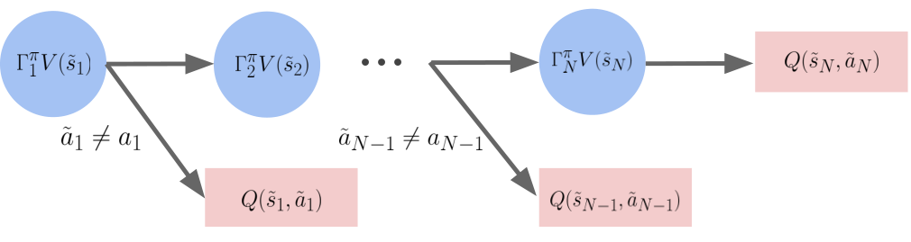
To actually estimate during off-policy training without access to the environment for and , we use the technique introduced in Section 4.2 to sample a path from the root to a leaf on the binary tree, by re-using the historical trajectory as much as possible. Specifically, we first set and as in the typical 1-step TD learning setting. Starting from , we sample and compare with . If they are equal, we continue to set and . We repeat this process until . In a word,
Usually for a continuous policy , is 1 with a probability of 1 because two sampled actions are always unequal. So will stop expanding at and it seems no more than just a normal Bellman operator for 1-step TD learning. However, if is specially structured and has a way of generating two identical actions in a continuous space, then it has the privilege of entering deeper tree branches for multi-step TD learning. For example, TAAC is indeed able to generate identical to the rollout action if , for all . In this case, .
Here we note that the above point estimate of can also be written as , where
Thus it shares a very similar form with Retrace (Munos et al., 2016), except the traces are now binary values defined by action comparison.
L.2 Convergence proof
Given any historical trajectory from an arbitrary behavior policy, we first verify that is a fixed point of . When in Eq. 16, we have . Now assuming , we have
Thus finally we have for any .
To prove that is the unique fixed point of , we verify that is a contraction mapping on the infinity norm space of . Suppose we have two different Q instantiations and , we would like prove that after applying to them, becomes strictly smaller than before. Let be the current infinity norm, i.e., . Then we have
and for recursively
Finally,
Since the discount factor , we have proved that is a contraction mapping.
Importantly, this contraction holds for any historical trajectory , even though this trajectory differs each time for an operator transform. Namely, every operator transform step will bring and closer, regardless of the actual value of the historical trajectory referred to. Combining this with being a fixed point of , we have shown that any will converge to if we repeatedly apply to it.