Data-driven modeling of power networks∗
Abstract
We develop a non-intrusive data-driven modeling framework for power network dynamics using the Lift and Learn approach of [30]. A lifting map is applied to the snapshot data obtained from the original nonlinear swing equations describing the underlying power network such that the lifted-data corresponds to quadratic nonlinearity. The lifted data is then projected onto a lower dimensional basis and the reduced quadratic matrices are fit to this reduced lifted data using a least-squares measure. The effectiveness of the proposed approach is investigated by two power network models.
I INTRODUCTION
Power grid networks play a fundamental role in transferring power from generators to consumers. The high dimensional mathematical model of power networks makes it difficult to monitor, analyze and control these systems. To overcome this issue, we use model reduction approaches to replace the high dimensional power networks model with a lower dimensional one that approximates the original with high fidelity. There is a plethora of model reduction approaches applied to power networks, see, e.g., [10, 9, 22, 25, 31, 33] and the references therein.
Most (nonlinear) model reduction methods have an intrusive nature; in other words, they rely on the full order model operators to derive a reduced model via projection. However, in many situations one might not have access to full-order dynamics. Instead, only measurements of the underlying dynamics are available. Therefore, recently, non-intrusive model reduction methods (data-driven methods) have received great attention. These methods learn a model based on data and without explicitly having access to the full order model operators. Various methods have been used to construct a reduced model from data. While some approaches are based on the frequency-domain data (see, e.g., [23, 17, 16, 11, 2, 1, 14, 20]) the others use time-domain data (see, e.g., [19, 12, 32, 34, 21, 30]).
In this paper, we use the Lift and Learn approach [30] to learn a quadratic reduced model for nonlinear swing equations modeling power network dynamics. We identify a lifting map by adding auxiliary variables to the system state of swing equations such that the resulting dynamics have a quadratic structure. This lifting map is applied to data obtained by evaluating the swing equations. The lifted data is projected onto a lower dimensional basis. Then, lower dimensional quadratic matrix operators are fitted to this reduced lifted data by a least-squares operator inference procedure.
The remainder of this paper is organized as follows: In Section II, we present the nonlinear model of the swing equations and its corresponding nonlinear quadratic representation as well as the projection-based model reduction for quadraticized swing equations followed by Section III where we review the Lift and Learn approach of [30]. Section IV presents the proposed data-driven framework where we apply the Lift and Learn approach to learn a low dimensional quadratic model for swing equations. Section V illustrates the feasibility of our approach via numerical examples followed by conclusions in Section VI.
II Power grid networks
There are three most common models for describing a network of coupled oscillators: synchronous motor (), effective network () and structure-preserving (). The coupling dynamics between oscillators in each model is governed by swing equations of the form [26]
| (1) |
where is the angle of rotation for the th oscillator, and are inertia and damping constants, respectively, is the angular frequency for the system, is dynamical coupling between oscillator and , and is the phase shift in this coupling. Constants , and are computed by solving the power flow equations and applying Kron reduction. For further details, we refer the reader to, e.g., [26] and [18].
Define . Then, the second-order dynamic of a network of coupled oscillators as in (1) can be described as
| (2) | ||||
where , and are defined as
| (3) | ||||
and is such that its th component is
| (4) |
for . Also in (2), we have and is the output mapping chosen to represent the quantity of interest (output) .
II-A Quadratic representation of swing equations
A large class of nonlinear systems can be represented as quadratic-bilinear systems by introducing some new variables arising from the smooth nonlinearities of the system like exponential, trigonometric, etc.; see, e.g., [24, 15, 5] and the references therein.
Second-order model (1) inherently contains a quadratic nonlinearity due to the function. Using trigonometric identity and simplified notations for and , nonlinearity can be written as
| (5) | ||||
Equation (5) hints at which variables to choose for incorporating in a new state vector. Define a new state vector as
| (6) |
II-B Projection-based model reduction for quadraticized swing equations
The high dimensional dynamics of the power network in (2) leads to the immense size of its quadratic representation in (7), which leads to a huge computational burden in simulation and prediction of power network dynamics. Hence, it is desirable to construct a reduced order model that approximate the original one with acceptable accuracy. Therefore, the goal is to find a reduced model for (7) of dimension
| (12) | ||||
where , , , such that the reduced output is a good approximation of the full order model output .
Using a Petrov-Galerkin framework, we construct the model reduction bases () such that and the reduced matrices are obtained as
| (13) | ||||
It is clear that the quality of the reduced quadratic model (12) depends on the choice of model reduction bases and and there are various methods to obtain these reduction bases specifically tailored to quadratic-nonlinear dynamical systems; see, for example, [15], [7], [6], [4] and the references therein.
Obtaining the reduced order matrices in (13) requires the knowledge of the full order model, i.e., the high-dimensional full order matrices , and in (7) that may not always be available or easy to derive. In some cases, even though the reduced order matrices can no longer be obtained via intrusive projection-based model reduction as in (13), they can be inferred from data. We describe this approach next, which we will then employ in data-driven modeling for power network dynamics.
III Lift and Learn method for Quadratic models
The Lift and Learn approach [30] is a powerful data-driven approach that uses the simulation data from the original nonlinear model (without access to its full-order state-space representation) to learn a quadratic reduced-order approximation to it. First, the approach collects state trajectory data of the original nonlinear model. Next, it lifts the data by a proper problem-dependent mapping to a quadratic model, and project the lifted data onto a low-dimensional basis via singular value decomposition (SVD). Then, it fits the reduced quadratic operators to the data by the least-squares operator inference procedure [28].
To be more precise, consider the following nonlinear dynamical system of ordinary differential equations
| (14) |
where is the state, is the input, and is a nonlinear function. For the dynamics (14), collect state snapshot data and input trajectory data at the time samples for :
| (15) | ||||
Define a lifting map
| (16) |
such that in the lifted-state , the dynamics (14) can be written exactly as a quadratic model (7), as we did in (6) and (7) for the power network dynamics. Then, apply this lifting map on each column of state snapshot (15) to form the lifted snapshot:
| (17) |
Compute the economy-size singular value decomposition (SVD) of the lifted snapshot :
where and have orthonormal columns and is diagonal with the singular values of on the diagonal. (Here we assumed ; the case follows similarly.) Based on the decay of , choose a truncation index and use the leading columns of , denoted by , to construct the reduced lifted snapshot matrix
| (18) |
As we stated above, the goal is to learn a reduced quadratic approximation, as in (12), to the original nonlinear dynamics (14). It is clear from (12) that to infer the reduced operators , and , the reduced time derivative of state snapshot is also required in addition to the reduced state snapshot in (18). Time derivative snapshot can be obtained from the state snapshot (17) using a time derivative approximation [8], e.g., the forward Euler integration. Then, similar to (18), [30] obtains the reduced time derivative snapshot as
| (19) |
III-A Least-squares operator inference procedure
Given reduced state snapshot (18), its corresponding reduced time derivative data (19) and the input snapshot in (15), operator inference approach in [28] formulates the following least-squares minimization problem to obtain the reduced order matrices , , appearing in (12):
| (20) |
The least-squares problem (20) is linear in the unknown variables and . Hence, the minimization problem (20) can be transformed into solving the linear least-squares problem [28], [30]
| (21) |
with
| (22) | ||||
where is constructed as
| (23) |
where is the th column of and denotes the Kronecker product without the redundant/repeated terms [30]. For example, for , the standard Kronecker product yields while by removing the repeated term , we have .
Similarly, is the form of without redundancy such that we can construct from by splitting the values corresponding to the quadratic cross terms across the redundant terms. For example, for ,
The over-determined least-squares (21) has a unique solution for if has a full column rank [13]. It was also shown in [27] that (21) can be expressed as independent least-squares problems as
| (24) |
where is the MATLAB notation referring to the th column of .
In the following section, we show how the Lift and Learn approach of [30] can be applied for data-driven modeling of nonlinear swing equations in power networks.
IV Learning power networks model from data
Recall the second-order dynamics of power grid networks given in (2), which we repeat here:
| (2) | ||||
For this nonlinear model (2), our goal in this section is to infer a reduced quadratic model approximation, as in (12), using the data trajectories of , and input (without access to the full order operators , , , , and ) by employing the Lift and Learn approach [30] reviewed in Section III. In other words, the goal is to fit quadratic reduced order matrices , and to the reduced snapshot data.
For the nonlinear model (2) under investigation, let , and be, respectively, the snapshots of , and input at time instances :
| (25) | ||||
Recall that in (2), , thus in this setting, we have
The augmented state (6) reveals that for power networks, we should define the lifting map as
| (26) |
Then, using in (26), the lifted data matrix is obtained as
| (27) | ||||
The time derivative data snapshot is also computed as explained in Section III.
The resulting data-driven modeling approach for nonlinear power networks (2) via Lift and Learn is summarized in Algorithm (1).
In situations where the coefficient matrix in (22) is rank-deficient, [35] proposes to regularize the least-squares problem (24) with an regularization as
| (28) |
for where is the regularization tuning parameter that controls a trade-off between solutions that fit the data well and solutions with a small norm. Regularization avoids over-fitting and improves the conditioning of the problem as well as the stability of the reduced order model. As we discuss in the next section, for the power network models we have studied, we have frequently encountered this situation in our numerical examples and had to employ the regularization process in our implementation.
V Numerical example
The two test systems we investigate are the SM model of the IEEE 118 bus system with and the EN model of IEEE 300 with , included in the MATPOWER software toolbox [36], [37]. We focus on the single-output system and thus . We choose the output, quantity of interest, as the arithmetic mean of all phase angles . In both case, we obtain the data via a numerical simulation with the time step size and the regularization tuning parameter . The inferred reduced order is chosen based on the singular value decay of the snapshot data with a relative tolerance of . In our simulations, we have employed the operator inference source code provided in [29].
V-A Example 1: IEEE 118 bus
We collect the data snapshots for the time interval seconds. With a step size of , this leads to the snapshot matrix . Based on the singular value decay of as shown in Figure 1 and the relative truncation tolerance of , we choose and form the projection basis .

Based on the reduced lifted data and , and the input snapshot , resulting coefficient matrix is rank-deficient with . Therefore, we solve the regularized least-squares problem (28) with . Using Algorithm 1, we find the data-driven quadratic reduced matrices , and in (12). To test the accuracy of the inferred model, we compare full-order model output with the reduced quadratic output in Figure 2. As the figure illustrates, the data-driven reduced quadratic model of order , obtained without access to original power network dynamics, accurately approximates the full model output.

Define the norm of the output as
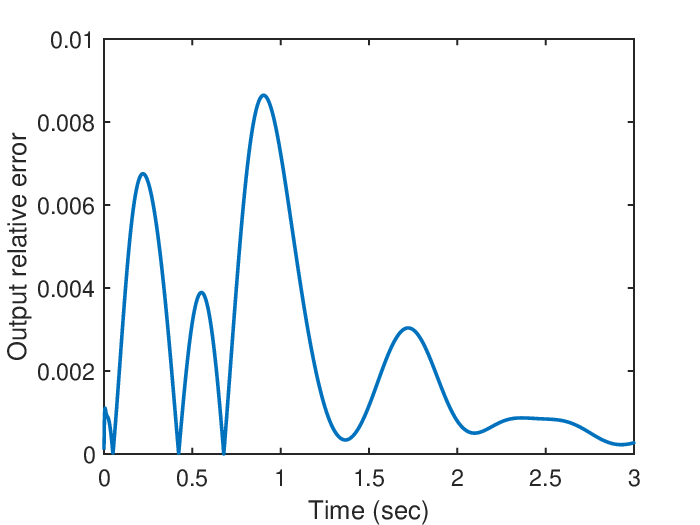
The relative output error
is shown in Figure 3. Figure 3 illustrates that, the learned model achieves a relative error of less than with a reduced order .
V-B Example 2: IEEE 300
In this example, we use EN model of IEEE 300 with . We collect the data snapshots for the time interval and obtain the snapshot matrix . Based on the singular value decay depicted in Figure 4, we choose . As in the previous example, the coefficient matrix is rank-deficient (). Hence, we solve (28) with to infer the reduced operators , , .

The outputs of the full-order and the reduced quadratic models are shown in Figure 5, once again illustrating an accurate match of the power network output via the learned model.

Figure 6 illustrates relative output error over the simulation time. According to the figure, the reduced model successfully approximate the full model with a relative output error less than over the time-interval seconds.

VI CONCLUSIONS AND FUTURE WORK
This paper illustrates the application of a data driven model reduction approach, the so called Lift and Learn method, to power grid networks. The non-intrusive nature of this methods enables us to infer a quadratic reduced model for the nonlinear swing equations using time domain data. Two examples have been used to demonstrate the the efficiency of our approach.
There are various interesting future directions to pursue. In this paper, the learned model is a reduced quadratic system and thus does not preserve the original second-order structure of the swing equations. Learning a reduced-structured model is a natural next step. Also, in this paper, the data for our data-driven approach has been obtained via numerical simulation. Testing the robustness of the approach on the noisy real measurements, such Phasor Measurement Unit data, will be crucial. Both directions are currently under investigation.
References
- [1] A. C. Antoulas, C. Beattie, and S. Güğercin. Interpolatory methods for model reduction. Computational Science and Engineering 21. SIAM, Philadelphia, 2020.
- [2] A. Astolfi. Model reduction by moment matching for linear and nonlinear systems. IEEE Transactions on Automatic Control, 55(10):2321–2336, 2010.
- [3] S. Gugercin B. Safaee. Structure-preserving model reduction for power network swing equations. SIAM Conference on Computational Science and Engineering, 2021.
- [4] P. Benner and T. Breiten. Two-sided moment matching methods for nonlinear model reduction. Preprint MPIMD/12-12, Max Planck Institute Magdeburg, June 2012. Available from http://www.mpi-magdeburg.mpg.de/preprints/.
- [5] P. Benner and T. Breiten. Two-sided projection methods for nonlinear model order reduction. SIAM Journal on Scientific Computing, 37(2):B239–B260, 2015.
- [6] P. Benner and P. Goyal. Balanced truncation model order reduction for quadratic-bilinear control systems. e-print 1705.00160, arXiv, 2017. math.OC.
- [7] P. Benner, P. Goyal, and S. Gugercin. -quasi-optimal model order reduction for quadratic-bilinear control systems. SIAM Journal on Matrix Analysis and Applications, 39(2):983–1032, 2018.
- [8] P. Benner, P. Goyal, B. Kramer, B. Peherstorfer, and K. Willcox. Operator inference for non-intrusive model reduction of systems with non-polynomial nonlinear terms. Computer Methods in Applied Mechanics and Engineering, 372:113433, 2020.
- [9] X. Cheng and J. MA Scherpen. Clustering approach to model order reduction of power networks with distributed controllers. Advances in Computational Mathematics, 44(6):1917–1939, 2018.
- [10] J. H. Chow. Power system coherency and model reduction, volume 84. Springer, 2013.
- [11] Z. Drmač, S. Gugercin, and C. Beattie. Quadrature-based vector fitting for discretized approximation. SIAM Journal on Scientific Computing, 37(2):A625–A652, 2015.
- [12] F. Giri and E.-W. Bai, editors. Block-oriented Nonlinear System Identification. Lecture Notes in Control and Information Sciences. Springer-Verlag, London, 2010.
- [13] G. H. Golub and C. F. Van Loan. Matrix computations, 1996.
- [14] I. V. Gosea and A. C. Antoulas. Data-driven model order reduction of quadratic-bilinear systems. Numerical Linear Algebra with Applications, 25(6):e2200, 2018. e2200 nla.2200.
- [15] C. Gu. Qlmor: A projection-based nonlinear model order reduction approach using quadratic-linear representation of nonlinear systems. IEEE Transactions on Computer-Aided Design of Integrated Circuits and Systems, 30(9):1307–1320, 2011.
- [16] B. Gustavsen and A. Semlyen. Rational approximation of frequency domain responses by vector fitting. IEEE Transactions on Power Delivery, 14(3):1052–1061, 1999.
- [17] A. C. Ionita and A. C. Antoulas. Data-driven parametrized model reduction in the loewner framework. SIAM Journal on Scientific Computing, 36(3):A984–A1007, 2014.
- [18] T. Ishizaki, A. Chakrabortty, and J. Imura. Graph-theoretic analysis of power systems. Proceedings of the IEEE, 106(5):931–952, 2018.
- [19] A. Juditsky, H. Hjalmarsson, A. Benveniste, B. Delyon, L. Ljung, J. Sjöberg, and Q. Zhang. Nonlinear black-box models in system identification: Mathematical foundations. Automatica, 31(12):1725 – 1750, 1995.
- [20] P. Kergus, F. Demourant, and C. Poussot-Vassal. Identification of parametric models in the frequency-domain through the subspace framework under lmi constraints. International Journal of Control, 93(8):1879–1890, 2020.
- [21] B. Kramer and K. E. Willcox. Nonlinear model order reduction via lifting transformations and proper orthogonal decomposition. AIAA Journal, 57(6):2297–2307, 2019.
- [22] M. H. Malik, D. Borzacchiello, F. Chinesta, and P. Diez. Reduced order modeling for transient simulation of power systems using trajectory piece-wise linear approximation. Advanced Modeling and Simulation in Engineering Sciences, 3(1):31, Dec 2016.
- [23] A. J. Mayo and A. C. Antoulas. A framework for the solution of the generalized realization problem. Linear Algebra and its Applications, 425(2):634–662, 2007. Special Issue in honor of Paul Fuhrmann.
- [24] G. P. McCormick. Computability of global solutions to factorable nonconvex programs: Part i—convex underestimating problems. Mathematical programming, 10(1):147–175, 1976.
- [25] P. Mlinarić, T. Ishizaki, A. Chakrabortty, S. Grundel, P. Benner, and J. Imura. Synchronization and aggregation of nonlinear power systems with consideration of bus network structures. In 2018 European Control Conference (ECC), pages 2266–2271, 2018.
- [26] T. Nishikawa and A. E Motter. Comparative analysis of existing models for power-grid synchronization. New Journal of Physics, 17(1):015012, jan 2015.
- [27] B. Peherstorfer and K. Willcox. Dynamic data-driven reduced-order models. Computer Methods in Applied Mechanics and Engineering, 291:21–41, 2015.
- [28] B. Peherstorfer and K. Willcox. Data-driven operator inference for nonintrusive projection-based model reduction. Computer Methods in Applied Mechanics and Engineering, 306:196 – 215, 2016.
- [29] E. Qian. Operator inference. https://github.com/elizqian/operator-inference, 2019.
- [30] E. Qian, B. Kramer, B. Peherstorfer, and K. Willcox. Lift & learn: Physics-informed machine learning for large-scale nonlinear dynamical systems. Physica D: Nonlinear Phenomena, 406:132401, 2020.
- [31] T. K. S. Ritschel, F. Weiß, M. Baumann, and S. Grundel. Nonlinear model reduction of dynamical power grid models using quadratization and balanced truncation. at - Automatisierungstechnik, 68(12):1022–1034, 2020.
- [32] C. W. Rowley., I. Mezi, S. Bagheri, P. Schlatter, and Dan S. H. Spectral analysis of nonlinear flows. Journal of Fluid Mechanics, 641:115–127, December 2009.
- [33] B. Safaee and S. Gugercin. Structure-preserving model reduction of parametric power networks. e-print 2102.05179, arXiv, 2021. eess.SY.
- [34] P. J. Schmid. Dynamic mode decomposition of numerical and experimental data. Journal of Fluid Mechanics, 656:5–28, 2010.
- [35] R. Swischuk, B. Kramer, C. Huang, and K. Willcox. Learning physics-based reduced-order models for a single-injector combustion process. AIAA Journal, 58(6):2658–2672, 2020.
- [36] R. D. Zimmerman and C. E. Murillo-Sánchez. Matpower 6.0 user’s manual. Power Systems Engineering Research Center, 9, 2016.
- [37] R. D. Zimmerman, C. E. Murillo-Sánchez, and R. J. Thomas. Matpower: Steady-state operations, planning, and analysis tools for power systems research and education. IEEE Transactions on power systems, 26(1):12–19, 2010.