A friendly introduction
to Fourier analysis on polytopes
and the geometry of numbers
Acknowledgements
The famous saying “no man is an island” is doubly-true in Mathematics, and indeed I’ve had the good fortune to know and learn from many interesting people, concerning the contents of this book. Special thanks goes to Ricardo Diaz, my first collaborator along these topics. I would like to thank the following people, from the bottom of my heart, for their valuable input and interesting discussions about some of these topics over the years:
Ian Alevy, Artur André, Christine Bachoc, Tamar Bar, Imre Bárány, Alexander Barvinok, Matthias Beck, Dori Bejleri, Luca Brandolini, Michel Brion, Sunil Chetty, Henry Cohn, Leonardo Colzani, Amalia Culiuc, Pierre Deligne, Jesús A. De Loera, Holley Friedlander, Michel Faleiros, Brett Frankel, Lenny Fukshansky, Nick Gravin, Tom Hagedorn, Martin Henk, Didier Henrion, Roberto Hirata Junior, Jeffrey Hoffstein, Judy Holdener, Alex Iosevich, Michael Joswig, Gil Kalai, Marvin Knopp, Mihalis Kolountzakis, Matthias Köppe, Greg Kuperberg, Jean Bernard Lasserre, Nhat Le Quang, Rafael Zuolo Coppini Lima, Sameer Iyer, Fabrício Caluza Machado, Romanos Malikiosis, Máté Matolci, Tyrrell McAllister, Nathan McNew, Paul Melvin, Victor Moll, Mel Nathanson, James Pommersheim, Jim Propp, Thales Paiva, Jill Pipher, Geremias Polanco, Jorge Luis Ramírez Alfonsín, Ethan Reiner, Bruce Reznick, Tiago Royer, Nicolas Salter, Gervásio Santos, Richard Schwartz, Dima Shiryaev, Joseph Silverman, Richard Stanley, Irena Swanson, Stephanie Treneer, Christophe Vignat, Sergei Tabachnikov, Karen Taylor, Giancarlo Travaglini, Mckenzie West, Ian Whitehead, Kevin Woods, Ren Yi, Günter Ziegler, Chuanming Zong.
Chapter 1 Once upon a time…..an introduction

What is a Fourier transform? Why is it so useful? How can we apply Fourier transforms and Fourier series - which were originally used by Fourier to study heat diffusion - in order to better understand topics in discrete and combinatorial geometry, number theory, and sampling theory?
To begin, there are some useful analogies: imagine that you are drinking a milk-shake (lactose-free), and you want to know the ingredients of your tasty drink. You would need to filter out the shake into some of its most basic components. This decomposition into its basic ingredients may be thought of as a sort of “Fourier transform of the milk-shake”. Once we understand each of the ingredients, we will also be able to restructure these ingredients in new ways, to form many other types of tasty goodies. To move the analogy back into mathematical language, the milkshake represents a function, and each of its basic ingredients represents for us the basis of sines and cosines; we may also think of a basic ingredient more compactly as a complex exponential , for some . Composing these basic ingredients together in a new way represents a Fourier series.
1.1 Introduction
Mathematically, one of the most basic kinds of milk-shakes is the indicator function of the unit interval, and to break it down into its basic components, Mathematicians, Engineers, Computer scientists, and Physicists have used the sinc function (since the ’s):
with great success, because it happens to be the Fourier transform of the unit interval :
as we will compute shortly in identity (3.3). Somewhat surprisingly, comparatively little energy has been given to some of its higher dimensional extensions, namely those extensions that arise naturally as Fourier transforms of polytopes.
One motivation for this book is to better understand how this -dimensional function – which has proved to be extremely powerful in applications – extends to higher dimensions. Namely, we will build various mathematical structures that are motivated by the question:
| What is the Fourier transform of a polytope? |
Of course, we will ask “how can we apply it”? An alternate title for this book might have been:
We’re taking Poisson summation and Fourier transforms of polytopes
for a very long ride….
Historically, sinc functions were used by Shannon (as well as Hardy, Kotelnikov, and Whittaker) when he published his seminal work on sampling theory and information theory.
In the first part of this book, we will learn how to use the technology of Fourier transforms of polytopes in order to prove some of Minkowski’s basic theorems in the geometry of numbers, to build the (Ehrhart) theory of integer point enumeration in polytopes, and to understand when a polytope tiles Euclidean space by translations.
In the second portion of this book, we give some applications to active research areas which are sometimes considered more applied, including the sphere-packing problem, and the sampling of signals in higher dimensions.
There are also current research developments of the material developed here, to the learning of deep neural networks. In many applied scientific areas, in particular radio astronomy, computational tomography, and magnetic resonance imaging, a frequent theme is the reconstruction of a function from knowledge of its Fourier transform. Somewhat surprisingly, in various applications we only require very partial/sparse knowledge of its Fourier transform in order to reconstruct the required function, which may represent an image or a signal.
One of the goals here is to allow the general mathematical reader to approach the forefront of modern research in this expanding area, and even tackle some of its unsolved problems. There is a rapidly increasing amount of research focused in these directions in recent years, and it is therefore time to put some of these new findings in one place, making them much more accessible to a general scientific reader.
The fact that the sinc function is indeed the Fourier transform of the -dimensional line segment , which is a -dimensional polytope, gives us a first hint that there is a deeper link between the geometry of a polytope and the analysis of its Fourier transform.
Indeed one reason that sampling and information theory, as initiated by Claude Shannon, works so well is precisely because the Fourier transform of the unit interval has this nice form, and even more-so because of the existence of the Poisson summation formula.
The approach we take here is to gain insight into how the Fourier transform of a polytope can be used to solve various specific problems in discrete geometry, combinatorics, optimization, approximation theory, and the Shannon-Whittaker sampling theory in higher dimensions:
- 1.
Analyze tilings of Euclidean space by translations of a polytope
- 2.
Give wonderful formulas for volumes of polytopes
- 3.
Compute discrete volumes of polytopes, which are combinatorial approximations to the continuous volume
- 4.
Introduce and develop the geometry of numbers, via Poisson summation
- 5.
Optimize sphere packings, and get bounds on their optimal densities
- 6.
Study the Shannon-Whittaker sampling theorem and its higher-dimensional siblings
Let’s see at least one direction that quickly motivates the study of Fourier transforms. In particular, we often begin with simple-sounding problems that arise naturally in combinatorial enumeration, discrete and computational geometry, and number theory.
Throughout, an integer point is any vector , all of whose coordinates are integers. In other words, belongs to the integer lattice . A rational point is a point whose coordinates are rational numbers, in other words . We define the Fourier transform of a function :
| (1.1) |
defined for all for which the latter integral converges, and where we use the standard inner product . We will also use the notation for the Fourier transform of , which is useful in some typographical contexts, for example when considering .
We introduce one of the main objects of study in this book, the Fourier transform of a polytope , defined by:
| (1.2) |
where the function is the indicator function of , defined by
Thus, the words “Fourier transform of a polytope ’’ will always mean the Fourier transform of the indicator function of .
1.2 The Poisson summation formula

The Poisson summation formula, named after Siméon Denis Poisson, tells us that for any “sufficiently nice” function we have:
| (1.3) |
In particular, if we were to naively set , the indicator function of a polytope , then we would get:
| (1.4) |
which is technically false for functions, due to the fact that the indicator function is discontinuous on .
However, this technically false statement is very useful! We make this claim because it helps us build intuition for the more rigorous statements that are true, and which we study in later chapters. For applications to discrete geometry, we are interested in the number of integer points in a closed convex polytope , namely . The combinatorial-geometric quantity may be regarded as a discrete volume for . From the definition of the indicator function of a polytope, the left-hand-side of (1.4) counts the number of integer points in , namely we have by definition
| (1.5) |
On the other hand, the right-hand-side of (1.4) allows us to compute this discrete volume of in a new way. This is great, because it opens a wonderful window of computation for us in the following sense:
| (1.6) |
We notice that for the term, we have
| (1.7) |
and therefore the discrepancy between the continuous volume of and the discrete volume of is
| (1.8) |
showing us very quickly that indeed is a discrete approximation to the classical Lebesgue volume , and pointing us to the task of finding ways to evaluate the transform . From the trivial but often very useful identity
we see another important motivation for this book: the Fourier transform of a polytope is a very natural extension of volume. Computing the volume of a polytope captures a bit of information about , but we also lose a lot of information.
On the other hand, computing the Fourier transform of a polytope uniquely determines , so we do not lose any information at all. Another way of saying this is that the Fourier transform of a polytope is a complete invariant. In other words, it is a fact of life that
Combinatorially, there are brilliant identities (notably the Brion identities) that emerge between the Fourier and Laplace transforms of a given polytope, and its facets and vertex tangent cones.
In Statistics, the moment generating function of any probability distribution is given by a Fourier transform of the indicator function of the distribution, hence Fourier transforms arise very naturally in Statistical applications. At this point, a natural glaring question naturally comes up:
| (1.9) |
And how do we use such computations to help us understand the important “error” term
that came up naturally in (1.8) above?
There are many applications of the theory that we will build-up. Often, we find it instructive to sometimes give an informal proof first, because it brings the intuitive ideas to the foreground, allowing the reader to gain an overview of the steps. Later on, we revisit the same intuitive proof again, making all of the steps rigorous.
The Poisson summation formula is one of our main stars, and some of its variations have relatively easy proofs. But it constitutes a very first step for many of our explorations.
1.3 Possible course outlines for teachers
There is enough content here for semesters, so it may be useful to outline some possible trajectories for a one-semester course:
[First option] Here the professor may follow an introduction to very basic Fourier analysis and then focus on the classical geometry of numbers, which may work well even for advanced undergraduates. To save time, one can begin with Chapters 2, 3, and in Chapter 4 only cover Sections 4.1 - 4.15, which includes the important Poisson summation II, á la Poisson himself, as well as convolutions. Then, one can cover:
Chapter 5.1: Sections 5.1 - 5.8 offer a novel introduction to the geometry of numbers.
Chapter 6: introduces the bread-and-butter of lattices, but covering only Sections 6.1 - 6-7 may be sufficient.
Chapter 7: this is a brief chapter that gives more theorems in the classical geometry of numbers, mainly the elegant theorems of Blichfeldt and Remak.
Chapter 8: basic Fourier transforms techniques are applied to recover a classical formula of Brion, for the Fourier transform of a simple polytope, via its vertex description.
[Second option] As a more advanced course, it’s also possible to go more deeply into the Fourier transforms of polytopes. I would recommend commencing with Chapters 2, 3, and parts of 4, and a bit of Chapter 6 on lattices, to give the basics of Fourier analysis, as well as sufficient intuition and motivation for what follows. Then one can cover:
Chapter 8: gives some detailed and complete formulas for the Fourier transform of a polytope, given its vertex description (a formula of Brion).
Chapter 9: introduces and develops the extension of a -dimensional angle (often called a solid angle) to higher dimensions.
Chapter 10: gives a discretized version of Brion’s theorem, for the integer point transform of a polytope, a discretized version of the Fourier transform of a polytope. Chapter 10 sets the stage for the Ehrhart theory of Chapter 11, which is an important theory that studies discrete volumes of polytopes.
The good news is that Chapters 11, 12, 13, 14, and 15 are essentially independent of each other. So there is a choice of ending the course with:
Chapter 12: Stokes’ theorem and its application to the Fourier transform of a polytope,
or Chapter 13: more advanced topics in the geometry of numbers that use theta functions,
or Chapter 14: Sphere packings, with upper bounds given by Poisson summation,
or Chapter 15: Shannon’s sampling theory in one and several variables, using Poisson summation.
1.4 Prerequisites
A word about prerequisites for this book: Linear Algebra is always very useful! A couple of calculus courses are required as well, with some real analysis. In particular, familiarity with infinite series is assumed. We give new proofs for some of the main theorems in this theory, including Theorem 5.4, Theorem 8.2, Theorem 8.3, and Theorem 10.1. Corollary 8.4 is one of the new results that appear in this book, which may also prove useful in extending the study of zero sets of the Fourier transform. These new Fourier-type proofs help streamline the theory, unifying sporadic results in the literature. This unifying thread will hopefully help the reader put the various results - from antiquity to modernity - into context.
We will assume some familiarity with the basic definitions of polytopes and their faces, although at places we will remind the reader of some of these definitions. There are many excellent texts that introduce the student to the classical language of polytopes, in particular the two classics: Günter Ziegler’s “Lectures on Polytopes” [253], and Branko Grünbaum’s “Convex Polytopes” [98]. For an easy introduction to the interactions between polytopes and lattice point enumeration, the reader is invited to consult “Computing the continuous discretely: integer point enumeration in polytopes”, by Beck and Robins [24]. But the contents of the latter book are not necessary for the study of the current book.
The level of the current book is aimed at advanced undergraduates and beginning graduate students in various fields, and in particular Mathematics, Computer Science, Electrical Engineering, and Physics. But I’ve included some goodies here and there for researchers as well. Indeed, one of the goals of this book is to allow the reader to rapidly reach the forefront of research in this area.
Because of the large number of exercises, with solutions to many of them in the back, this book can also be used effectively for self-study. If an exercise is marked with a symbol, it means that we’ve mentioned this exercise in the body of the text, for that chapter. Finally, this book is still in draft form, and in particular Chapters 10, 11, 12, and 15, are still under revision.
We proceed by developing an intuitive understanding first, using many examples and analogies, and this intuition then points us to a rigorous path for the details of the ensuing proofs.
Sinai Robins February 2023
IME, University of São Paulo
Chapter 2 A motivating problem:
tiling a rectangle with rectangles
“Ripping up carpet is easy – tiling is the issue”.
– Douglas Wilson

2.1 Intuition
To warm up, we begin with a simple tiling problem in the plane. A rectangle will be called nice if at least one of its sides is an integer. We prove a now-classical fact about tiling a rectangle with nice rectangles, namely Theorem 2.1, and we focus on the method of the straightforward proof.
This proof brings to the foreground an important idea: by simply taking a Fourier transform of a body , we immediately get interesting geometric consequences for . In particular, we will see throughout this book various ways in which the Fourier transform of a geometric body is a natural extension of its volume, sometimes in a continuous way, and sometimes in a discrete way. So in order to study relationships between volumes of bodies, it is very natural and useful to play with their Fourier transforms.
2.2 Nice rectangles
The tilings that we focus on, in this small chapter, are tilings that are composed of smaller rectangles, all of which have their sides parallel to the axes, and all of which are nice. There are at least different known proofs [246] of Theorem 2.1. Here we give the proof that uses very basic Fourier tools, from first principles, motivating the chapters that follow. The idea for this proof goes back to Nicolaas Govert De Bruijn [63].
Theorem 2.1 (De Bruijn).
Suppose we tile a fixed rectangle with smaller, nice rectangles.
Then is a nice rectangle.
Proof.
Suppose that the rectangle is tiled with smaller rectangles , as in Figure 2.1. Due to our tiling hypothesis, we have
| (2.1) |
where the notation always means we are using indicator functions. To ease the reader into the computations, we recall that the Fourier transform of the indicator function of any rectangle is defined by:
| (2.2) |
Now we may formally take the Fourier transform of both sides of (2.1). In other words we simply multiply both sides of (2.1) by the exponential function and then integrate both sides over , to get:
| (2.3) |
In (2.3), we have used the fact that a -dimensional integral over a -dimensional line segment always vanishes, due to the fact that a line segment has measure relative to the -dimensional measure of the -dimensional transform. Let’s compute one of these integrals, over a generic rectangle :
| (2.4) | ||||
| (2.5) | ||||
| (2.6) | ||||
| (2.7) | ||||
| (2.8) |
valid for all except for the union of the two lines and . Considering the latter formula for the Fourier transform of a rectangle, we make the following leap of faith:
Claim. Suppose that is a rectangle whose sides are parallel to the axes. Then
| (2.9) |
Proof of the claim. We consider the last equality (2.8). We see that
| (2.10) |
which is equivalent to having either , or . But we know that due to Euler, if and only if (Exercise 2.1), so we have
| (2.11) |
Now, if is a nice rectangle, then one of its sides is an integer, say without loss of generality. Therefore
for , and by (2.11), we see that
.
Conversely, if we assume that , then by
(2.11) either
, proving the claim.
To finish the proof of the theorem, by hypothesis each little rectangle is a nice rectangle, so by the claim above it satisfies . Returning to (2.3), we see that therefore , for , and using the claim again (the converse part of it this time), we see that must be nice. ∎
The proof of Theorem 2.1 was simple and elegant, motivating the use of Fourier transforms of polytopes in the ensuing chapters. The claim, namely equation (2.9), offers an intriguing springboard for deeper investigations - it tells us that we can convert a geometric statement about tiling into a purely analytic statement about the vanishing of a certain integral transform. Later, when we learn about Theorem 5.5, we will see that this small initial success of (2.9) is part of a larger theory. This is the beginning of a beautiful friendship…….
2.3 Conventions, and some definitions
We mention some conventions that we use throughout the book. First, we note that whenever we are given a complex-valued function , we may write in terms of its real and imaginary parts: . The integral of such an is defined by
| (2.12) |
so that all of our Fourier transforms are really reduced to the usual integration of real-valued functions on Euclidean space (see Exercise 2.4). This is good news for the reader, because even though we see complex functions in the integrand, elementary calculus suffices.
Let be a set. For our purposes, we may call a measurable set if the integral and in this case we define
Equivalently, we may call measurable if the indicator function is an integrable function, by definition of the (Lebesgue) integral. We’ll use the fact that every open set, every closed set (and hence every compact set) is measurable [202]. A set is said to have measure zero if
In , for example, we may alternatively define a set of measure as follows. Given any , there exists a countable collection of open intervals that cover all of , and whose total length satisfies . But we will assume the reader knows the definition(s) of an integral (either the Riemann integral or the Lebesgue integral), circumventing discussions about -algebras of sets, so that the background required of the reader is kept to a minimum.
The point we want to make here is that most things are in fact easier than the reader may have previously thought.
We say that a statement concerning points holds for almost every (we also use the words almost everywhere) if the set of for which is false is a set of measure . For example, we have the following fact from real analysis:
which means that for almost every .
We also mention our convention/notation for some definitions. Whenever we want to define a new object called , in terms of some combination of previously known mathematical objects called , we will use the standard notation
For any set , we define the closure of as the the smallest (w.r.t containment) closed set that contains , written as . We define the interior of as the set of all points such that there exists a ball of some positive radius , centered at , with . We define the boundary of , written as , by
An important concept is that of the support of a function , defined by
| (2.13) |
With this definition, we have for example:
We will also say that a function is compactly supported if the support of is a compact set . In particular this means that vanishes outside of .
Notes
- 1.
This little chapter was motivated by the lovely article written by Stan Wagon [246], which gives different proofs of Theorem 2.1. The article [246] is important because it shows - in a concrete manner - how tools from one field can leak into another field, and may therefore lead to important discoveries in the future.
- 2.
In a related direction, we might wonder which polygons, and more generally which polytopes, tile Euclidean space by translations with a lattice. It turns out (Theorem 5.5) that this question is equivalent to the statement that the Fourier transform of vanishes on a (dual) lattice.
- 3.
In the context of the Hilbert space of functions , Exercise 2.3 is one step towards showing that the set of exponentials forms an orthonormal basis for . Namely, the identity above shows that these basis elements are orthogonal to each other - their inner product vanishes for integers . Thus, the identity of Exercise 2.3 is often called the orthogonality relations for exponentials, over . To show that they span the space of functions in is a bit harder, but see [239] for details.
- 4.
The question in Exercise 2.16 for was originally asked by Paul Erdős in , and has an affirmative answer. This question also has higher-dimensional analogues:
Suppose we give a partition of the integer lattice into a finite, disjoint union of translated sublattices. Is it always true that at least two of these sublattices are translates of each other?
The answer is known to be false for , but is still unsolved for (see [82],[42]).
Exercises
“The game’s afoot”
– Arthur Conan Doyle (in his book Sherlock Holmes)
2.1.
Show that if , then if and only if .
2.2.
Show that , for all complex numbers .
2.3.
Here we prove the orthogonality relations for the exponential functions defined by , for each integer . Recall that the complex conjugate of any complex number is defined by
so that for all real . Prove that for all integers :
| (2.14) |
2.4.
Here the reader may gain some practice with the definitions of integrals that use complex-valued integrands . We recall for the reader the following definition:
| (2.15) |
a linear combination of two real-valued integrals. Recalling that by definition,
show directly from definition 2.15 and from Euler’s identity , that for any nonzero , we have
Notes. Another way of thinking about this exercise is that it extends the ‘Fundamental theorem of calculus’ to complex-valued functions in a rather easy way. The anti-derivative of the integrand is , and we are saying that it is ok to use it in place of the usual anti-derivative in Calculus - it is consistent with definition 2.15. In the future, we generally do not have to break up complex integrals into their real and imaginary parts, because we can make use of the fact that antiderivatives of complex-valued functions are often simple, such as the one in this example.
We also note that this is not calculus with a complex variable, because the domains of our integrands, as well as the measures we are using throughout this book, are defined over real Euclidean space . This means we are still using basic Calculus.

2.5.
We recall that the ’th roots of unity are by definition the set of complex solutions to , and are given by the set of points on the unit circle. Prove that the sum of all of the ’th roots of unity vanishes. Precisely, fix any positive integer , and show that
2.6.
Prove that, given positive integers , we have
Notes. This result is sometimes referred to as “the harmonic detector” for detecting when a rational number is an integer; that is, it assigns a value of to the sum if , and it assigns a value of to the sum if .
2.7.
Here we prove the orthogonality relations for roots of unity. Namely, fix any two nonnegative integers , and prove that
| (2.16) |
Notes. In a later chapter on Euclidean lattices (Chapter 6), we will see that the identity 2.16 is a special case of the more general orthogonality relations for characters on lattices. From this perspective, this exercise gives the orthogonality relations on the finite cyclic group . There are more general orthogonality relations for characters of group representations, which play an important role in Number Theory.
2.8.
Show that for any positive integer , we have
where .
2.9.
An ’th root of unity is called a primitive root of unity if it is not a ’th root of unity for some smaller positive integer . Show that the primitive ’th roots of unity are precisely the numbers for which .
2.10.
The Möbius -function is defined by:
Prove that the sum of all of the primitive ’th roots of unity is equal to the Möbius -function, evaluated at :
| (2.17) |
Notes. See problem 5.24, as a way of intertwining the Möbius -function with Poisson summation.
2.11.
We follow the Weierstrassian approach to defining the complex exponential for all complex :
| (2.18) |
which converges absolutely for all . We also have the (Weierstrassian) definitions of and :
both converging absolutely again for all . Using these three Taylor series in , prove that Euler’s formula has the extension:
valid for all .
Notes. Beginning with such a power series approach to many of the standard functions, Karl Weierstrass developed a rigorous and beautiful theory of real and complex functions.
2.12.
Here the reader needs to know a little bit about the quotient of two groups (this is one of the few exercises that assumes group theory). We prove that the group of ‘real numbers mod ’ under addition, is isomorphic to the unit circle, under multiplication of complex numbers. Precisely, we can define by .
- 1.
We recall the definition of the kernel of a map, namely . Show that .
- 2.
Using the first isomorphism Theorem for groups, show that is isomorphic to the unit circle .
2.13.
Using gymnastics with roots of unity, we recall here a very classical solution to the problem of finding the roots of a cubic polynomial.
- 1.
Let , and show that we have the polynomial identity:
- 2.
Using the latter identity, solve the cubic polynomial: by substituting and .
2.14.
Thinking of the function as a function of a complex variable , show that its zeros are precisely the set of integers .
2.15.
Here we give another equivalent condition for a rectangle in Theorem 2.1 to be a nice rectangle, using the same definitions as before.
Let’s call a generic integer point if is not orthogonal to any of the edges of . In other words, a generic integer vector satisfies , for all , and in particular is not generic, nor is any point on the -axis or the -axis. Then
| (2.19) |
2.16 Erdős, 1951.
Erdős asked: “Can the set of all positive integers be partitioned (that is, written as a disjoint union) into a finite number of arithmetic progressions, such that no two of the arithmetic progressions will have the same common difference?”
Precisely, suppose that we have
| (2.20) |
for some positive integers , and , and where the arithmetic progressions are pairwise disjoint.
Prove that in any such partitioning of the integers, (that is, the largest common difference must appear at least twice).
Notes. For example, if we write , a disjoint union of arithmetic progressions, then we see that the largest common difference of appears twice. Erdős noticed that such a phenomenon must always occur. (See also Exercise 13.12 for an extension to lattices in ).
2.17.
Continuing with the ideas of Exercise 2.16, suppose we are given a disjoint union of arithmetic progressions such as (2.20) above.
- 1.
Prove that:
(2.21) - 2.
Show further that for all indices .
- 3.
Conversely, suppose that we are given positive integers , with for all indices , and such that . Can we always find integers , such that we have the following disjoint union of arithmetic progressions: ? (as in (2.20))
Chapter 3 Examples nourish the theory
“To many, mathematics is a collection of theorems. For me, mathematics is a collection of examples; a theorem is a statement about a collection of examples and the purpose of proving theorems is to classify and explain the examples…”
– John B. Conway
“A pint of example is worth a gallon of advice.”
– Anonymous

3.1 Intuition
One way to think about the Fourier transform of a polytope is that it simultaneously captures all of the moments of , thereby uniquely defining . Here we begin concretely by computing some Fourier transforms of various polytopes in dimensions and , as well as the Fourier transforms of some simple families of polytopes in dimension as well.
The -dimensional computations will get the reader more comfortable with the basics. In later chapters, once we learn a little more theory, we will return to these families of polytopes and compute some of their Fourier transforms in general.
We also see, from small examples, that the Bernoulli polynomials immediately enter into the picture, forming natural building blocks. In this chapter we compute Fourier transforms without thinking too much about convergence issues, to let the reader run with the ideas. But commencing with the next chapter, we will be more rigorous when using Poisson summation, and with convergence issues.
3.2 Dimension - the classical sinc function
We begin by computing the classical -dimensional example of the Fourier transform of the symmetrized unit interval :
For all , we have:
| (3.1) | ||||
| (3.2) | ||||
| (3.3) |
Noticing that is a removable singularity, we define the continuous sinc-function by
| (3.4) |
which is in fact infinitely smooth, via Lemma 3.1 below.

3.3 The Fourier transform of as a complete invariant
The main goal of this section is to state Lemma 3.2, which tells us that all of the information about a polytope is contained in its Fourier transform. To that end, we introduce the inverse Fourier transform, often called the Fourier inversion formula. We’d like to see the fundamental fact that under certain conditions, the Fourier transform is invertible. First, we call a function absolutely integrable if , and we write this as .
Theorem 3.1.
Given a function such that both and , we have
| (3.5) |
for all .
(see [78] for a proof). We’ll also use the notation . Equation (3.5) tells us that the inverse Fourier transform exists, and is almost equal to itself. A moment’s thought reveals that we may rewrite (3.5) in the following useful form:
| (3.6) |
Example 3.1.
A famous and historically somewhat tricky integral formula for the sinc function is the following fact:
| (3.7) |
also known as the Dirichlet integral. The careful reader might notice that the latter integrand is not absolutely convergent, which means that (Exercise 3.23). So we have to specify what we really mean by the identity (3.7). The rigorous claim is:
Let’s see an intuitive derivation of (3.7), where we will be fast-and-loose for the moment. Using (3.2), we’ve seen above that the Fourier transform of the indicator function of the interval is:
| (3.8) |
so that
| (3.9) |
Using the definition of the Fourier transform, the latter identity is:
| (3.10) |
and now evaluating both sides at gives us (3.7). Although this derivation appears very convincing, it would not make it past the rigor police (see also note 6). So why not? It is because we applied the Fourier inversion formula to a function that was not in , namely the sinc function. So we owe it to ourselves to pursue a rigorous approach by showing that
| (3.11) |
whose validity would give us a variation on Fourier inversion, for a function that is not in , namely . This is tricky business, but such an endeavor is taken up in Exercise 3.36.
We can extend Example 3.1 in a natural way to all Fourier pairs of functions, , provided that we may apply Fourier inversion, as follows. Simply let in (3.5), to get:
| (3.12) |
Another nice and very useful fact about the Fourier transform of a polytope is that it is an entire function, meaning that it is differentiable everywhere. This differentiability is already observable in the sinc function above, with its removable singularity at the origin.
Lemma 3.1.
Let be a -dimensional polytope. Then is an entire function of .
Proof.
Because is compact, we can safely differentiate under the integral sign (this is a special case of Lebesgue’s Dominated Convergence Theorem). Namely, for the coordinate variable , we have: . Since one complex derivative of now exists (in the complex variable ), the function is analytic in , and using the same reasoning it is also analytic in each of the variables . ∎
We also have the very fortuitous fact that the Fourier transform of any polytope is a complete invariant, in the following sense. We recall that by definition a polytope is in particular a closed set.
Lemma 3.2.
Let be a polytope. Then uniquely determines . Precisely, given any two -dimensional polytopes , we have
In other words, for any polytope , its Fourier transform uniquely determines the polytope.
Proof.
(outline) If , it is clear that for all . Conversely, suppose that for all . Using Fourier inversion, namely Theorem 3.1, we may take the Fourier transform of both sides of the latter equation to get , for all . ∎
The reason that the proof above is only an outline - at this point - is due to the fact that we have applied the Fourier inversion formula (3.5) to , which is not an absolutely integrable function (as we’ll see in Corollary 4.3 in even greater generality).
We’ll revisit Lemma 3.2 in Chapter 4, as Theorem 4.3 for a rigorous proof. In fact much more is true - see note 2. There is also a nice version of the Fourier inversion formula, due to Podkorytov and Minh, which is related [184]. The reason we’ve put Lemma 3.2 so early in the text is because it offers an extremely strong motivation for the study of Fourier transforms of polytopes, showing that they are complete invariants.
A fascinating consequence of Lemma 3.2 is that when we take the Fourier transform of a polytope, then all of the combinatorial and geometric information of is contained in the formula of its Fourier transform……somehow. So we may begin to create a complete dictionary between the geometry and combinatorics of a polytope in the space domain, and its Fourier transform in the frequency domain.
3.4 Bernoulli polynomials
We introduce the Bernoulli polynomials, which turn out to be a sort of “glue” between discrete geometry, number theory, and Fourier analysis, as we will see throughout the book. Historically, Jacob Bernoulli was considering the formulas
and so on. Jacob was wondering how to find a general formula for the sums:
With hindsight giving us slightly better vision, the modern approach to the latter polynomials begins with the following generating function:
| (3.13) |
It follows from this definition (3.13) that each coefficient is a polynomial in , of degree (Exercise 3.4). These polynomials are called Bernoulli polynomials, and Bernoulli was able to show that in general:
for all integers and (Exercise 3.8). The reader can develop her skills by proving some of the surprising and important properties of Bernoulli polynomials in Exercises 3.4 through 3.18.
Example 3.2.
The first few Bernoulli polynomials are:
| (3.14) | ||||
| (3.15) | ||||
| (3.16) | ||||
| (3.17) | ||||
| (3.18) | ||||
| (3.19) | ||||
| (3.20) |
It turns out that it’s very useful to periodize the Bernoulli polynomials, in the following sense. We first define:
the fractional part of . Now we define the ’th periodic Bernoulli polynomial:
| (3.21) |
for . Since is periodic on with period , it has a Fourier series, and it turns out that
| (3.22) |
valid for (Exercise 3.9). When , we have the first Bernoulli polynomial
which is very special (see Figure 3.1). For one thing, is the only periodic Bernoulli polynomial that is not continuous everywhere, and we note that its Fourier series does not converge absolutely, although it is quite appealing:
| (3.23) |
valid for all . But how are we supposed to sum up a conditionally convergent series such as (3.23)? A common way to define it rigorously is to prove that
As we can see, special care must be taken with , and Exercise 3.34 provides a rigorous proof of the convergence of (3.23). The Bernoulli numbers are defined to be the constant terms of the Bernoulli polynomials:
Perusing Example 3.2, we see that the
first few Bernoulli numbers are:
It follows quickly from definition 3.13 above that for odd , (Exercise 3.15). Using the generating function 3.13, the Bernoulli numbers are defined via
| (3.24) |
An interesting identity that allows us to compute the Bernoulli numbers recursively is:
valid for all (Exercise 3.17). Some of the most natural, and beautiful, Fourier series arise naturally from the periodized Bernoulli polynomials.
Recalling the statement of Poisson summation (1.3) from the Introduction, we now give a fast-and-loose application in dimension . The following intuitive application of the Poisson summation formula already suggests an initial connection between periodized Bernoulli polynomials and Fourier transforms of polytopes.
Example 3.3 (Intuitive Poisson summation).
In this example we allow ourselves to be completely intuitive, and unrigorous at this moment, but often such arguments are useful in pointing us to their rigorous counterparts. Consider the -dimensional polytope , and restrict attention to the case of . If we could use the Poisson summation formula
applied to the function , then we would get:
We’ve used quotation marks around the latter string of equalities because the sums are formally divergent. But we already know how to evaluate the left-hand side of Poisson summation above, namely . So we’ve confirmed that Poisson summation has given us the correct formula here, in spite of the lack of rigor at this point. We also see rather quickly why the first periodic Bernoulli polynomial appears so naturally in integer point enumeration in polytopes, from this perspective.
Why is the intuitive argument above not rigorous yet? In order to plug a function into Poisson summation, and consider convergence at each point of the domain, and its Fourier transform must both satisfy some growth conditions at infinity, at the very least ensuring proper convergence of both sides of the Poisson summation formula. We will see such conditions later, in Chapter 4, Theorem 4.13. After we learn how to use Poisson summation, we will return to this example, which will become rigorous in Section 9.4.
We recall that a series is said to converge absolutely if converges. It’s easy to see that the series in (3.23) for does not converge absolutely. Such convergent series that do not converge absolutely are called conditionally convergent.
3.5 The cube, and its Fourier transform
Perhaps the easiest way to extend the Fourier transform of the unit interval is to consider the -dimensional unit cube
What is its Fourier transform? When we compute a Fourier transform of a function , we will say that is a Fourier pair. We have seen that is a Fourier pair in dimension .
Example 3.4.
Due to the fact that the cube is the direct product of line segments, it follows that the ensuing integral can be separated into a product of integrals, and so it is the product of -dimensional transforms:
| (3.25) | ||||
| (3.26) | ||||
| (3.27) | ||||
| (3.28) |
valid for all such that none of their coordinates vanishes. So here we have the Fourier pair
In general, though, polytopes are not a direct product of lower-dimensional polytopes, so we will need to develop more tools to compute their Fourier transforms.
3.6 The simplex, and its Fourier transform
Another basic building block for polytopes is the standard simplex, defined by
| (3.29) |
Example 3.5.
Just for fun, let’s compute the Fourier transform of for , via brute-force. We may use the following parametrization (called a hyperplane description) for this standard triangle:
Hence, we have:
We may simplify further by noticing the rational function identity
giving us the symmetric function of :
| (3.30) |
3.7 Convex sets and polytopes
We need the concept of a convex set , defined by the property that for any two points , the line segment joining them also lies in . In other words, the line segment , .
Given any finite set of points , we can also form the set of all convex linear combinations of by defining
| (3.31) |
Given any set (which is not restricted to be finite, or bounded), we define the convex hull of as the set of convex linear combinations, taken over all finite subsets of , and denoted by .
We define a polytope as the convex hull of any finite set of points in . This definition of a polytope is called its vertex description. We define a -simplex as the convex hull of a finite set of vectors :
where , and are linearly independent vectors in . The points are called the vertices of , and this object is one of the basic building-blocks of polytopes, especially when triangulating a polytope.
The simplex is a -dimensional polytope, sitting in . When , the dimension of equals the dimension of the ambient space - see Figure 3.4.

We have already computed the Fourier transform of a particular -simplex, in (3.30).
How do we define a face of a polytope more precisely? To begin, a hyperplane is defined by
for any fixed vector , and any . A hyperplane is called a supporting hyperplane for if lies on one side of , in the precise sense that:
We now call a face of if , for some supporting hyperplane of . As a consequence of the latter definition, the empty set is also a face of , because we may pick a hyperplane very far from , which does not intersect . As a separate definition, we define to be a face of itself.
With these preliminaries, we’re now ready to compute the Fourier transform of any -simplex in . In order to handle a general triangle, let be any triangle in the plane, with vertices
Can we reduce the computation of to our already known formula for , given by (3.30)? We first notice (after a brief cup of coffee) that we can map any triangle in the plane to the standard triangle, by using a linear transformation followed by a translation:
| (3.32) |
where is the matrix whose columns are and . We are now ready to compute the Fourier transform of a general triangle :
Making the substitution , with , we have , and so
where we’ve used our formula (3.30) for the FT of the standard triangle (thereby bootstrapping out way to the general case) with , and . Substituting these values into the latter expression, we finally arrive at the FT of our general triangle :
| (3.33) |
We can notice in equation (3.33) many of the same patterns that had already occurred in Example 3.9. Namely, the Fourier transform of a triangle has denominators that are products of linear forms in , and it is a finite linear combination of rational functions multiplied by complex exponentials.
Also, in the particular case of equation (3.33), is a symmetric function of , as we might have expected.
Using exactly the same ideas that were used in equation (3.33), it is possible to prove (by induction on the dimension) that the Fourier transform of a general -dimensional simplex is:
| (3.34) |
where the vertex set of is (Exercise 3.29), and in fact the same formula persists for all complex such that the products of linear forms in the denominators do not vanish.
However, looking back at the computation leading to (3.33), and the corresponding computation which would give (3.34), the curious reader might be thinking:
“There must be an easier way!”
But never fear - indeed there is. So even though at this point the computation of may be a bit laborious (but still interesting), computing the Fourier transform of a general simplex will become quite easy once we will revisit it in a later chapter (see Theorem 8.2).
3.8 Stretching and translating
The perspicacious reader may have noticed that in order to arrive at the formula (3.33) above for the FT of a general triangle, we exploited the fact that the Fourier transform interacted peacefully with the linear transformation , and with the translation by the vector . Is this true in general?
Indeed it is, and we record these thoughts in the following two lemmas, which will become our bread and butter for future computations. In general, given any invertible linear transformation , and any function whose FT (Fourier transform) exists, we have the following useful interaction between Fourier transforms and linear transformations.
Lemma 3.3 (Stretch).
| (3.35) |
Proof.
By definition, we have We perform the change of variable , implying that , so that:
∎
What about translations? They are even simpler.
Lemma 3.4 (Translate).
For any translation , where is a fixed vector, we have
| (3.36) |
Proof.
Again, by definition we have so that performing the simple change of variable , we have . The latter integral becomes
∎
In general, any function of the form
| (3.37) |
where is a fixed linear transformation and is a fixed vector, is called an affine transformation. For example, we’ve already seen in (3.32) that the right triangle was mapped to the more general triangle by an affine transformation. So the latter two lemmas allow us to compose Fourier transforms very easily with affine transformations.
Example 3.6.
The simplest example of the Stretch Lemma 3.3 is obtained in , where the matrix , a positive real number. So we have . Considering as a function of , we have by (3.36):
| (3.38) |
As an interesting sub-example, let’s take , for a fixed constant . What’s the easy way to use the Stretch lemma to compute ? First, we have to make a slight conversion: . Using the FT of the unit interval, equation (3.3), together with (3.38), we have:
| (3.39) |
Example 3.7.
Consider any set , for which is integrable, and let’s translate by a fixed vector , and compute .
We note that because , the translate lemma applies, but with a minus sign. That is, we can use and to get:
| (3.40) |
3.9 The parallelepiped, and its Fourier transform
Now that we know how to compose the FT with affine transformations (translations and linear transformations), we can easily find the FT of any parallelepiped in by using our formula for the Fourier transform of the unit cube , which we derived in Example 3.4:
| (3.41) |
for all such that all the coordinates of do not vanish. First, we translate the cube by the vector , to obtain
It’s straightforward to compute its FT as well (Exercise 3.2), by using Lemma 3.4, the ‘translate’ lemma:
| (3.42) |
Next, we define a -dimensional parallelepiped as an affine image of the unit cube. In other words, any parallelepiped has the description
for some linear transformation , and some translation vector . Geometrically, the cube is stretched and translated into a parallelepiped.

For the sake of concreteness, will will first set and compute the Fourier transform of , where we now give as a invertible matrix whose columns are . Because the cube may be written as a convex linear combination of the basis vectors , we see that may be written as a convex linear combination of . In other words, we see that the (closed) parallelepiped has the equivalent vertex description:
To review the basics, let’s compute the FT of our parallelepiped from first principles:
| (3.43) | ||||
| (3.44) | ||||
| (3.45) | ||||
| (3.46) |
where in the third equality we used the substitution , with , yielding . In the last equality, we used our known formula (3.42) for the FT of the cube , together with the elementary linear algebra fact that the ’th coordinate of is given by .
Finally, for a general parallelepiped, we have , so that by definition
Noting that , we compute the Fourier transform of by using the ‘translate lemma’ (Lemma 3.4), together with formula (3.46) for the Fourier transform of :
| (3.47) |
for all , except for those that are orthogonal to one of the (which are edge vectors for ).
Example 3.8.
A straightforward computation shows that if we let , then is symmetric about the origin, in the sense that (Exercise 3.25). In other words, the center of mass of this new is now the origin. Geometrically, we’ve translated the previous parallelepiped by using half its ‘body diagonal’. For such a parallelepiped , centered at the origin, formula (3.47) above gives the more pleasing expression:
| (3.48) | ||||
| (3.49) | ||||
| (3.50) | ||||
| (3.51) |
To summarize, for a parallelepiped that is symmetric about the origin, we have the Fourier pair
We could have also computed the latter FT by beginning with our known Fourier transform (3.41) of the cube , composing the FT with the same linear transformation of (3.43), and using the ‘stretch’ lemma, so everything is consistent.
3.10 The cross-polytope
Another natural convex body in is the cross-polytope
| (3.52) |
In dimension , the cross-polytope can be defined similarly by its hyperplane description
| (3.53) |
The cross-polytope is also, by definition, the unit ball in the -norm on Euclidean space, and from this perspective a very natural object. In , the cross-polytope is often called an octahedron.
In this section we only work out the -dimensional case of the Fourier transfrom of the crosspolytope, In Chapter 8, we will work out the Fourier transform of any -dimensional cross-polytope, , because we will have more tools at our disposal.
Nevertheless, it’s instructive to compute via brute-force for here, in order to gain some facility with the computation of Fourier transforms.
Example 3.9.
Using the definition of the Fourier transform, we first compute the FT of the -dimensional cross polytope:
| (3.54) |
In , we may write as a union of the following triangles:
Since these four triangles only intersect in lower-dimensional subsets of , the -dimensional integral vanishes on such lower dimensional subsets, and we have:
| (3.55) |
Recalling from equation (3.30) of example 3.5 that the Fourier transform of the standard simplex is
| (3.56) |
we can compute , by reflecting about the (the Jacobian of this transformation is ), and using the already-computed transform (3.56) of :
Similarly, we have , and .
Hence we may continue the computation from equation 3.55 above, putting all the pieces back together:
| (3.57) | ||||
| (3.58) | ||||
| (3.59) | ||||
| (3.60) | ||||
| (3.61) | ||||
| (3.62) | ||||
| (3.63) |
It’s time to mention another important relationship between the cross-polytope and the cube . To see this relationship, we define, for any polytope , its polar polytope:
| (3.64) |
It is an easy fact (Exercise 3.26) that in , the cross-polytope and the cube are polar to each other, as in Figure 3.7.

In many applications, it turns out the the volume of the cross-polytope plays an important role. So we compute it here, for a generalized cross-polytope defined by the image of under any invertible linear transformation , whose ’th olumn is defined by :
| (3.65) |
Lemma 3.5.
With the notation above, we have
- 1.
- 2.
- 3.
In particular, if , then we have
Proof.
To prove part 1, we can simply triangulate the crosspolytope into isometric simplices by using the coordinate planes. Each such simplex has volume , so we’re done. For part 2, we have:
| (3.66) |
where we used the change of variable and its ensuing Jacobian transformation . The last equality above follows from part 1. Part 3 follows trivially from part 2, using the determinant of a diagonal matrix. ∎
3.11 Observations and questions
Now we can make several observations about all of the formulas that we found so far, for the Fourier transforms of various polytopes. For the -dimensional cross-polytope, we found that
| (3.67) |
- 1.
It is real-valued for all , and this is due to the fact that is symmetric about the origin (see section 5.6).
Question 1.
Is it true that any symmetric property of a polytope is somehow mirrored by a corresponding symmetric property of its Fourier transform?
Although this question is not well-defined at the moment (it depends on how we define ‘symmetric property’), it does sound exciting, and we can morph it into a few well-defined questions later.
- 2.
- 3.
- 4.
The denominators of all of the FT’s so far are always products of linear forms in .
Question 2.
[Rhetorical] Is it true that the Fourier transform of any polytope is always a finite sum of rational functions times an exponential, where the denominators of the rational functions are always products of linear forms?
Answer: (spoiler alert) Yes! It’s too early to prove this here, but we’ll do it in the course of proving Theorem 8.3.
- 5.
We may retrieve the volume of by letting and tend to zero (Exercise 3.21), as always. Doing so, we obtain
Notes
- 1.
Another way to compute for the -dimensional cross-polytope is by starting with the square and applying a rotation of the plane by , followed by a simple dilation. Because we know that linear transformations interact in a very elegant way with the FT, this method gives an alternate approach for the Example 3.9 in .
However, this method no longer works for the cross-polytope in dimensions , where it is not (yet) known if there is a simple way to go from the FT of the cube to the FT of the cross-polytope.
More generally, one may ask:
Question 3.
is there a nice relationship between the FT of a polytope and the FT of its polar?
- 2.
With regards to Lemma 3.2, much more is true. If the Fourier transforms of any two compact sets agree on any convergent sequence (with a finite limit point), then . The reason is that here and are both entire functions of , so the proof follows from the identity theorem in complex variables.
- 3.
We note that is defined to be equal to at the integers, because its Fourier series naturally converges to the mean of the discontinuity of the function, at each integer.
- 4.
It has been known since the work of Riemann that the Bernoulli numbers occur as special values of the Riemann zeta function (see Exercise 4.4). Similarly, the Hurwitz zeta function, defined for each fixed by
has a meromorphic continuation to all of , and its special values at the negative integers are the Bernoulli polynomials (up to a multiplicative constant).
- 5.
There are sometimes very unusual (yet useful) formulations for the Fourier transform of certain functions. Ramanujan ([190], eq. (2)) discovered the following remarkable formula for the Fourier transform of the Gamma function:
(3.68) valid for .
For example, with , in the language of this chapter we have the Fourier pair . But from the -function identity (3.73) below (extended to a complex variable ), it quickly follows that . So this special case of allows us to conclude the interesting fact that is a fixed point of the Fourier transform.
- 6.
I borrowed this joke from [178], a nice and informal introduction to Fourier analysis.
Exercises
Problems worthy of attack prove their worth by fighting back.
– Paul Erdős
3.1.
Show that the Fourier transform of the closed interval is:
for .
3.2.
Show that the Fourier transform of the unit cube is:
| (3.69) |
valid for all , except for the union of hyperplanes defined by
.
3.3.
Suppose we are given two polynomials and , of degree . If there are distinct points in the complex plane such that for , show that the two polynomials are identical. (Hint: consider )
3.4.
To gain some facility with generating functions, show by a brute-force computation with Taylor series that the coefficients on the right-hand-side of equation (3.13), which are called by definition, must in fact be polynomials in .
In fact, your direct computations will show that for all , we have
where is the ’th Bernoulli number.
3.5.
Show that for all , we have
3.6.
Show that for all , we have
3.7.
Show that for all , we have
3.8.
Prove that:
for all integers and .
3.9.
Show that the periodic Bernoulli polynomials , for all , have the following Fourier series:
| (3.70) |
valid for all . For , these series are absolutely convergent. We note that from the definition above, when .
3.10.
Show that the greatest integer function (often called the ‘floor function’) enjoys the property:
for all , and all positive integers .
3.11.
Show that the Bernoulli polynomials enjoy the following identity, proved by Joseph Ludwig Raabe in 1851:
for all , all positive integers , and for each .
Notes. Such formulas, in these last two exercises, are also called “multiplication Theorems”, and they hold for many other functions, including the Gamma function, the dilogarithm, the Hurwitz zeta function, the cotangent, and many more.
3.12.
Here we give a different method for defining the Bernoulli polynomials, based on the following three properties that they enjoy:
- 1.
.
- 2.
For all .
- 3.
For all , we have .
Show that the latter three properties imply the original defining property of the Bernoulli polynomials (3.13).
3.13.
Here is a more explicit, useful recursion for computing the Bernoulli polynomials. Show that
for all .
3.14.
Use the previous exercise, together with the known list the first Bernoulli polynomials that appear in equation 3.20, to compute .
3.15.
Show that for odd , we have .
3.16.
Show that the even Bernoulli numbers alternate in sign. More precisely, show that
for each positive integer .
3.17.
Show that the Bernoulli numbers enjoy the recursive property:
for all .
3.18.
Show that the Bernoulli numbers enjoy the following asymptotics:
as . Here we are using the usual notation for asymptotic functions, namely that as if .
3.19.
Show that the following integrals converge and have the closed forms:
| (3.71) | ||||
| (3.72) |
Notes. These integrals are called Fresnel integrals, and they are related to the Cornu spiral, which was created by Marie Alfred Cornu. Marie used the spiral as a tool for computing diffraction patterns that arise naturally in optics.
3.20.
Prove the following Gamma function identity, using the sinc function:
| (3.73) |
for all .
Notes. This identity is often called Euler’s reflection formula. is by definition the Gamma function, where the integral converges for all (see Section 5.8 for more on the function).
3.21.
Using the formula for the Fourier transform of the -dimensional cross-polytope , derived in the text, namely
find the area of by letting in the latter formula.
3.22.
Some elementary but very useful bounds for trig functions are developed here.
- 1.
Prove that
where the left inequality holds for , and the right inequality holds for .
- 2.
Prove that
where the left inequality holds for , and the right inequality holds for .
- 3.
Prove that
where the left inequality holds for , and the right inequality holds for .
3.23.
Show that .
Notes. Once we have the inverse Fourier transform and its consequences at our disposal, this exercise will become trivial, and much more general - see Corollary 4.3.
3.24.
There are (at least) two different ways of periodizing a given function with respect to . First, we can define , so that is periodic on with period . Second, we may also define , which is also a periodic function on with period .
Find an absolutely integrable (meaning that converges) function for which these two functions are not equal: .
Notes. In Chapter 4, we will see that the latter function captures a lot more information about , and often captures all of as well.
3.25.
Given linearly independent vectors , let , and define , a parallelepiped. Show that is symmetric about the origin, in the precise sense that .
3.26.
Show that the -dimensional cross-polytope and the cube are polar to each other.
3.27.
- 1.
Suppose is a convex polytope with vertices. Prove that at least one of the vertices of has degree .
- 2.
Construct a convex polytope with vertices, such that all of its vertices have degree .
3.28.
Prove the following -dimensional integral formula:
| (3.74) |
valid for all such that .
3.29.
Using the ideas of Example 3.33, prove (by induction on the dimension) that the Fourier transform of a general -dimensional simplex is given by:
| (3.75) |
for all , where the vertex set of is .
3.30Abel summation by parts.
Here we prove the straightforward but very useful technique of Niels Abel, called Abel summation by parts. Suppose we are given two sequences , and . We define the finite partial sums . Then we have
| (3.76) |
for all .
Notes. Using the forward difference operator, it’s easy to recognize identity (3.76) as a discrete version of integration by parts.
3.31Dirichlet’s convergence test.
Suppose we are given a real sequence , and a complex sequence , such that
- 1.
is monotonically decreasing to , and
- 2.
, for some positive constant , and all .
Then converges.
3.32.
Prove that for all , we have the following important identity, called the ‘‘Dirichlet kernel’’, named after Peter Gustav Lejeune Dirichlet:
| (3.77) |
Notes. An equivalent way to write (3.77) is clearly:
3.33.
Prove that we have the bound on the following exponential sum:
| (3.78) |
for any fixed , and for all .
3.34.
Prove that converges, given any fixed .
Notes. We see that, although does not converge absolutely, Abel’s summation formula (3.76) gives us
and the latter series does converge absolutely, as . So we see that Abel summation transforms one series (that barely converges at all) into another series that converges more rapidly.
3.35.
Here we’ll prove that
| (3.79) |
in the sense that . The integral (3.79) is sometimes called “the Dirichlet integral”. Comparing this Dirichlet integral with Exercise 3.23, we see that there is something subtle going on here. We’ll end up proving something slightly more general here:
for all .
- 1.
Define
(3.80) for each . Justify differentiation under the integral sign, and show that
- 2.
Show that .
- 3.
Show that , and then show that the constant .
- 4.
Prove that is a continuous function of , and finally prove that
which is the desired result (Here you might want to integrate by parts first, and then use the Dominated convergence theorem).
Notes. There are many proofs of this famous identity (3.79), and although the method of contour integration is arguably the most straightforward, here we are only assuming knowledge of some real analysis. The expression in (3.80) is also known as the Laplace transform of the sinc function, and it is a variation of the Fourier transform that we will revisit when studying similar transforms of cones in Section 8.7.
3.36.
Here we give a rigorous proof of the tricky fact that for all , we have
following an approach taken by S. Bochner [39]. We begin by noticing that this integral can be easily reduced to a real-valued integral:
because for each , , owing to the oddness of the integrand.
- 1.
Using the result from Exercise 3.35, prove that
- 2.
Chapter 4 The basics of Fourier analysis
“If a function is periodic, then we should try to expand it into its Fourier series, and wonderful things will begin to happen…..”
– Erich Hecke
“. . . Fourier’s great mathematical poem.”
-- William Thomson Kelvin
[Referring to Fourier’s mathematical theory of the conduction of heat]

4.1 Intuition
Because we will use tools from Fourier analysis throughout, we introduce them here as an outline of the field, with the goal of applying them to the discrete geometry of polytopes, lattices, and their interactions. We will sometimes introduce a concept by using an intuitive argument, which we call “fast and loose”, but after such an intuitive argument, we state the precise version of the corresponding theorem. In this chapter, we will sometimes point to the literature for some of the proofs.
Our goal is to use the necessary tools of Fourier analysis in order to tackle problems in the enumerative combinatorics of polytopes, in number theory, discrete geometry, and in some other fields. We emphasize that the Poisson summation formula allows us to discretize integrals, in a sense that will be made precise in later chapters.
One pattern that the reader may have already noticed, among all of the examples of Fourier transforms of polytopes computed thus far, is that each of them is a linear combination of a very special kind of rational function of , multiplied by a complex exponential that involves a vertex of the polytope:
| (4.1) |
where the vertices of are , and where . We observed that in all of our examples thus far, the denominators are in fact products of linear forms, as in (4.1). We will be able to see some of the more precise geometric structure for these products of linear forms, which come from the edges of the polytope, once we learn more about Fourier-Laplace transforms of cones.
It is rather astounding that every single fact about a given polytope is somehow hiding inside these rational-exponential functions given by (4.1), due to the fact that the Fourier transform is a complete invariant (Lemma 3.2).
Finally, it is worth mentioning that not every fact in this chapter is necessary for the comprehension of the rest of the book. The reader is advised to learn just some of this chapter, and as she/he reads the rest of the book, periodically revisit this chaper.
4.2 Introducing the Fourier transform on
In the spirit of bringing the reader very quickly up to speed, regarding the applications of Fourier analytic tools, we outline the basics of the field, and prove some of them. Nowadays, there are many good texts on Fourier analysis, and the reader is encouraged to peruse some of these books (see Note 1).
Unless otherwise stated, all of our functions will have the form . One of the most useful tools for us is the Poisson summation formula. We provide several versions of Poisson summation, each of which uses a different set of sufficient conditions.
As we will see, the Fourier transform is a very friendly creature, allowing us to travel back and forth between the “space domain” and the “frequency domain” to obtain many useful results. The readers who are already familiar with basics of Fourier analysis may easily skip this chapter without impeding their understanding of the rest of the book. Although we enjoy thinking about the warm and cozy Hilbert spaces and , there are exotic Fourier series that are pointwise divergent, and yet represent continuous functions, a whole field onto itself. We won’t go there. However, the very basic convergence issues are still important for us as well, and we will study them because we want to get the reader up and running.
The function space that immediately come up very naturally is the the space of absolutely integrable functions on :
Secondly, the space of square-integrable functions on is defined by:
The usual theory of Fourier transforms progresses by first defining the Fourier transform for functions belonging to , which is quite a natural condition, and then later extending the Fourier transform to the space by taking appropriate limits. We initially restrict attention to functions .

There are many fascinating facts about all of these functions spaces. For practice, let’s ask:
Question 4.
[Rhetorical] Given two functions , is their product always in ?
Well, we have the Cauchy-Schwartz inequality for the Hilbert space :
| (4.2) |
the latter inequality holding by the assumption . So the product is indeed in , answering Question 4 in the affirmative. This is the first sign that there are fascinating links between functions and functions. In fact, this metaphorical dance between and is simply too useful to ignore, so we will use study some of the interactions between these two spaces, from first principles (see Section 4.17 below, for example).
The utility of the Cauchy-Schwarz inequality should never be underestimated, and holds in greater generality.
Lemma 4.1.
Let be an inner product space, with the inner product . Then the following Cauchy-Schwarz inequality holds:
for all . Moreover, equality holds and are linearly dependent. In addition, the function
is a norm on .
(For a proof see [78], Prop. 3.2. Appendix B.3 has some related material) So we can conclude from Lemma 4.1 that every inner product space is also a normed vector space. The converse is false, though, in the sense that there are normed vector spaces, whose norm does not arise from any inner product. One fascinating example of such a space is , which is not a Hilbert space, as we now easily show by exhibiting a counter-example to the Cauchy-Schwarz inequality.
Example 4.1.
We claim that the Cauchy-Schwarz inequality is false in . If the Cauchy-Schwarz inequality was true here, then (4.2) would be valid for all functions . But as a counterexample, let
It’s easy to see that :
But diverges, so that we do not have a Cauchy-Schwarz inequality in , because here both the left-hand-side and the right-hand-side of such an inequality do not even converge.
We say that is bounded on a measurable set by a constant , if , for all . In the opposite direction of Example 4.1, if two functions are bounded on , and absolutely integrable on , then we do have a Cauchy-Schwartz inequality for the pair , and we let the reader enjoy its verification.
We’ll see that despite the fact that is not a Hilbert space, it does have a very beautiful structure, namely it is a Banach algebra (Lemma 4.12).
4.3 The triangle inequality for integrals
An easy but extremely important inequality is the triangle inequality for integrals, as follows.
Theorem 4.1.
For any , and any measurable subset , we have:
| (4.3) |
Proof.
Letting , we may write , for a (unique) complex on the unit circle. We let be the real part of , so that . Altogether, we have:
| (4.4) |
In the third equality, we used the fact that is real, which follows from the first two equalities: . ∎
Although Theorem 4.1 seems innocently trivial, it is sometimes quite powerful.
Corollary 4.1.
If is bounded on a measurable set by a constant , then:
| (4.5) |
Proof.
where the first inequality uses the triangle inequality for integrals, namely Theorem (4.1), and the second inequality uses the boundedness assumption on . ∎
What about the equality case in Theorem 4.1? Luckily there is a very satisfying answer, which turns out to be so useful that it merits its own Corollary. We’ll keep using the same notation as in the proof of Theorem 4.1.
Corollary 4.2 (Equality conditions for the triangle inequality).
Let , fix any measurable subset , and suppose that
Then we have for some complex number on the unit circle, and for almost all .
Proof.
Returning to (4.4) in the proof of Theorem 4.1, our assumption of equality now gives us
| (4.6) |
We also have , so by (4.6) we now have , almost everywhere. Now we recall that is the real part of , with a complex number on the unit circle. So we have almost everywhere. Since , we see that almost everywhere. In other words, almost everywhere. ∎
Next, let’s show that
confirming the validity of set intersections in Figure 4.2. We’ll do it for , but the idea works for any dimension.
Example 4.2.
Let’s define
Then , because . But , because . So .
On the other hand, if we consider
then , because . But because . So .
We’ve defined the Fourier transform before, and we remind the reader that for any function , the Fourier transform of is
| (4.7) |
Where does this definition really come from? One motivation comes from the inner product for functions (in ), where we project a function onto each exponential function:
Another motivation comes from the proof of the Poisson summation formula - eq. (4.55) below, which shows a crucial connection between the Fourier transform of and the Fourier coefficients of the periodized function .
One of the first things we might notice is:
Claim 1.
The Fourier transform is a bounded linear operator.
The Fourier transform is a linear operator, by the linearity of the integral: , and it is a bounded operator due to the elementary estimate in Lemma 4.2 below.
A natural question is: where does the Fourier transform take a function ? An immediate partial answer is that for any , we have:
where is the space of bounded functions on . Here the constant depends only on . To see this, consider:
| (4.8) | ||||
| (4.9) |
where we used Theorem 4.1, the triangle inequality for integrals, together with the fact that . So we’ve just proved the following fact.
Lemma 4.2.
Given , its Fourier transform is uniformly bounded, with the following bound:
| (4.10) |
for all .
Example 4.3.
Let’s bound the Fourier transform of an indicator function , for any bounded measurable set :
In particular, for any polytope ,
We already know that , so it’s natural to ask whether the maximum allowed value of can also be achieved by a nonzero ; or perhaps it may be the case that we always have the strict inequality ? (See Exercise 4.25).
But a lot more is true for absolutely integrable functions.
Lemma 4.3.
If , then is uniformly continuous on .
Proof.
We fix any , and , and we compute:
so by the triangle inequality for integrals, we have
| (4.11) |
Letting , we see that
using . We may now use the dominated convergence theorem, because the functions are dominated by the absolutely integrable function . So we get:
Because the latter limit is independent of , (4.11) tells us that , as , uniformly in . ∎
It turns out that sometimes we need to measure distance between functions in a manner different than just pointwise convergence. We therefore introduce convergence in the norm. We say that a sequence of functions converges to a function in the norm if
| (4.12) |
for which we also use the notation . It is also very useful to define the spaces, for each :
| (4.13) |
which naturally extend the and spaces. In fact for functions , the function is a norm; it’s also a fact that for , this norm does not arise from an inner product. But of course, for this norm does arise from an inner product, via Lemma 4.1. It is well-known that among all of the spaces, the only one that is a Hilbert space is . For the curious reader, the other spaces, for , also possess some additional structure, namely they are Banach spaces, after identifying two functions that are equal a.e. (see [78] for details). The development of spaces is very important for Fourier analysis; for the sake of simplicity of exposition, here we will mostly work with and .
4.4 The Riemann–Lebesgue lemma
The celebrated Riemann–Lebesgue lemma gives us the basic decay property of the Fourier transform as . To prove it, we will use the fact that we can approximate any function with arbitrary precision by using ‘step functions’ in . More precisely, let a box in be defined by , and consider the indicator function of this box. If we consider the set of all finite sums, taken over all such indicator functions (varying over all boxes), with arbitrary real coefficients, then this set turns out to be dense in , in the norm. We record this fact as a lemma.
Lemma 4.4.
If , then there is a finite sum of indicator functions of boxes that approaches , in the norm.
Lemma 4.5 (Riemann-Lebesgue lemma).
If , then:
Proof.
We first show the result in the case that is the indicator function of a box. We already know, via Exercise 3.1, that if , then
| (4.15) |
As through a sequence of ’s with nonvanishing coordinates, we see that while the numerator of (4.15) stays bounded, the denominator satisfies . Hence we’ve proved the lemma for indicator functions of boxes. Since , we know by Lemma 4.4 that there exists a sequence of functions such that , as . Also, by (4.15) we know that this sequence already satisfies . Using the elementary inequality (4.10), we get:
as . Therefore . ∎
With all of the above properties, it is now natural to consider the space of all uniformly continuous functions on that go to at infinity:
| (4.16) |
So although the Fourier transform does not map the space into itself, all of the above results may be summarized as follows.
Lemma 4.6.
If , then .
4.5 The inverse Fourier transform
To invert the Fourier transform, we already mentioned briefly, in Theorem 3.1 and in example 3.1, an intuitive description of this process. Now we state things more formally.
Theorem 4.2 (The inverse Fourier transform).
If and , then
| (4.17) |
for all .
The reader is invited to see [78] for a proof. Almost all proofs proceed by introducing a Gaussian approximate identity inside the integrand of the inversion formula, then recognizing the integrand as a convolution with an approximate identity, and finally removing the approximate identity by invoking a limit, such as (4.113) below, at each point of continuity of .
The inverse Fourier transform is sometimes called ‘Fourier inversion’. Let’s see an interesting application, showing in particular that the Fourier transform of a polytope is not absolutely integrable.
Corollary 4.3.
Let be a compact set. Then .
Proof.
If is a convex set, for example, then we see that is not absolutely integrable, and we did not have to make any messy computations to see it. Of course, one of the most basic consequences of Fourier inversion is the uniqueness of transforms, as follows.
Corollary 4.4.
Suppose that , and that for all . Then almost everywhere.
Proof.
Letting , we clearly have . Let’s compute: for all . In particular , so that we may apply Fourier inversion:
almost everywhere. ∎
Now we can revisit our intuitive Lemma 3.2 and give a rigorous proof of a more general statement (see also note 2 in Chapter 3).
Theorem 4.3.
Let be a compact set. Then uniquely determines . Precisely, given any two -dimensional compact sets , we have
| (4.19) |
In particular, for any polytope , its Fourier transform uniquely determines the polytope.
Proof.
Suppose that . We apply Corollary 4.4 to the functions and , to conclude that for almost all . In other words, almost everywhere.
The latter statement implies that vanishes at each of its points of continuity. But is continuous on the whole interior of , and similarly for (they are both identically there). Therefore for all in the interior of and for all in the interior of . Also, for each , and for each . Therefore , and hence . ∎
Example 4.4.
What would happen if we assume less, and replace by a lattice, say ? Is it possible for the following phenomenon to occur:
| (4.20) |
Indeed this scenario can happen, but we need to learn about extremal bodies first (see Section 5.5).
4.6 The torus
Suppose a function is periodic on the real line, with period : , for all . Then we may think of as ‘living’ on the unit circle, via the map which wraps the real line onto the unit circle. In this setting, we may also think of the circle as the quotient group . As we promised, group theory will not be assumed of the reader, but it will be developed a little bit in the concrete context of lattices - see Section 6.4 as well.
We may also traverse these ideas in the other direction: commencing with any function whose domain is just , we can always extend by periodicity to the whole real line by defining , the fractional part of , for all . Then for all , is periodic on , and therefore we may think of as living on the circle .
More generally, we may think of a periodic function as living on the cube , if we insist that is periodic in the following sense:
In this case, the -dimensional circle is replaced by the -dimensional torus
which we may also think of as the unit cube , but with opposite facets ‘glued together’. Here we define another infinite-dimensional vector space, namely:
| (4.21) |
We notice that the domains of the integrals in are cubes, and hence always compact. So we may therefore expect nicer phenomena to occur in this space.
We also have the space of absolutely integrable functions on the torus:
| (4.22) |
which plays a simpler role than the analogous space we had before. And finally we also define the useful space of -differentiable functions on the torus:
| (4.23) |
As a special case, we’ll simply denote by the space of all continuous functions on the torus. We emphasize that by definition, all of the latter function spaces, , consist of periodic functions on the cube .
Similarly to the inner product on , we also have in this new context a natural inner product for the space of square-integrable functions , defined by:
| (4.24) |
making a Hilbert space. For each , we define by:
| (4.25) |
This countable collection of exponentials turns out to form a complete orthonormal basis for . The orthogonality is the first step, which we prove next. For the proof that the exponentials span and are complete, we refer the reader to [78].
Theorem 4.4 (Orthogonality relations for the exponentials on the torus).
| (4.26) |
Proof.
Because of the geometry of the cube, we can proceed in this case by separating the variables. If , then there is at least one index for which . We compute:
because is a nonzero integer. ∎
Because is also an inner product space, it still enjoys the Cauchy-Schwartz inequality. Intuitively, the space should be a cozier little space than . This intuition can be made more rigorous by the following Lemma, despite the fact that . More generally, given any compact and convex set , and any , we define
| (4.27) |
Lemma 4.7.
We have the following proper containments:
- 1.
.
- 2.
In general, given any compact and convex set , .
Proof.
Given , we must show that . Using the Cauchy-Schwartz inequality for , applied to and the constant function on , we have:
so we see that is absolutely integrable over the torus . To show that the containment in part 1 is proper, for , we can consider the following function on :
So , but . Hence , but .
4.6.1 Fourier series: fast and loose
Let’s see how we can expand (certain) functions in a Fourier series, as well as find a formula for their series coefficients, in a foot-loose and carefree way - i.e. abandoning all rigor for the moment.
Given that the sequence of exponential functions forms a basis for the infinite dimensional vector space , we know from Linear Algebra that any function may be written in terms of this basis:
| (4.28) |
How do we compute the Fourier coefficients ? Let’s go through the intuitive process here, ignoring convergence issues. Well, again by Linear Algebra, we take the inner product of both sides with a fixed basis element :
where we’ve used the orthogonality relations, Theorem 4.4 above, in the third equality. We also used the standard notation if , and if . Therefore, it must be the case that
also called the Fourier coefficients of .
4.6.2 Fourier series: slow and rigorous
Let’s record now the rigorous statements of the intuitive arguments that we constructed in the previous section. We may think of a periodic function on as a function belonging to .
Theorem 4.5 (Fourier series for functions on ).
The set of exponentials
form a complete orthonormal basis for . Moreover, we have the following:
- 1.
Every function has a Fourier series
(4.29) where the convergence in (4.29) takes place in the norm on the torus .
- 2.
The Fourier coefficients may be computed via the formula:
(4.30) for all .
- 3.
(The Parseval identity) The function in (4.29) satisfies
(4.31)
(For a proof, see [78], p. 96) At the risk of overstating the obvious, we note that the equality in (4.31) is simply equality between real numbers. We also note that the Fourier coefficients above are integrals over the unit cube , and may also be thought of as , the projection of onto each basis element. To summarize, we’ve encountered the following types of transforms so far:
| (4.32) |
To disambiguate, the first integral in (4.32) arises from periodic functions on , and it appears as a Fourier coefficient in Theorem 4.5. The second integral is our old friend the Fourier transform. How are the two integrals related to each other? This is exactly the magic of the Poisson summation formula, Theorem 4.12.
In the pretty proof of Poisson summation, we begin with a Fourier series of a periodized version of , and end up showing that its Fourier coefficients, by a small miracle of nature, turn out to also be Fourier transforms of .
A natural question is:
Question 5.
Which functions have a pointwise convergent Fourier series?
But this question turns out to be rather difficult, and many lifetimes have been devoted to related questions. It is a fact of life that the Fourier series of an arbitrary continuous function on may fail to converge uniformly, or even pointwise. However, there is some good news. As it turns out, if we impose some smoothness conditions on , then does have a Fourier series which converges pointwise, as we’ll see next.
4.7 Piecewise smooth functions have convergent Fourier series
In this section we’ll restrict attention to the real line. We’d like to rigorously define the intuitive idea of a function that is almost continuous, in the sense of being continuous on an interval except for finitely many finite jump discontinuities.
Precisely, given real numbers , we define a function to be piecewise continuous on if the following two conditions are met:
- 1.
is continuous on , except possibly on a finite set of points
- 2.
The left-hand and right-hand limits of exist at each of the points :
Furthermore, we define a function to be piecewise smooth on if both and its derivative are piecewise continuous on . We’ll also say that a function is piecewise continuous/smooth on if it is piecewise continuous/smooth on every finite interval. We have the following refined version of Theorem 4.5, on the real line.
Theorem 4.6.
Let be a periodic function, with domain , and piecewise smooth on . Then, for each , we have
| (4.33) |
where are the Fourier coefficients of .
We will come back to these partial Fourier sums, occurring in Theorem 4.6, and defined by
| (4.34) |
There is also a natural and easy extension of Parseval’s identity (4.31). Given any two functions , we’ve seen in (4.29) that
both converging in the norm.
Theorem 4.7.
If , then with the notation above we have
4.7.1 The first periodic Bernoulli polynomial
To see a concrete instance of Theorem 4.5, we study the function , which we’ve briefly encountered before, as the first periodic Bernoulli polynomial. This function turns out to be so important that it deserves its own section here. We recall its definition:
| (4.35) |
It’s easy to see that , so it has a Fourier series, by Theorem 4.5, part (a):
| (4.36) |
and the equality here means equality in the norm.

Let’s compute the Fourier coefficients of , according to Theorem 4.5, part (b). We will use integration by parts:
when . For , we have . Hence we have the Fourier series
| (4.37) |
where the latter equality means convergence in the norm. But we’d like pointwise convergence of the latter series! In fact, this follows from Theorem 4.6, as follows.
Corollary 4.5.
We have the pointwise convergent Fourier series
| (4.38) |
valid for all .
Proof.
Next, we can give a classical application of the Fourier series (4.37) using Parseval’s identity (4.31):
Let’s simplify both sides:
while
Therefore
a number-theoretic identity that goes back to Euler. In a similar manner one can evaluate the Riemann zeta function at all positive even integers, using the cotangent function (Exercise 4.4).
Another natural question arises.
Question 6.
What sort of functions are uniquely determined by all of their Fourier coefficients?
To describe a partial answer, we recall the space of all continuous functions on the torus:
| (4.41) |
Theorem 4.8.
Let , and suppose that for all . Then , for all .
In particular, if and for all , then for all .
In other words, a continuous function on the torus is uniquely determined by its Fourier coefficients (see [78] for a proof).
4.8 As gets smoother, decays faster
There is a very basic and important relationship between the level of smoothness of , and the speed with which tends to as . To capture this relation very concretely, let’s compute things on the real line, to see how the FT interacts with the derivative.
Lemma 4.8.
Let .
- 1.
If is piecewise smooth, and also enjoys , then:
- 2.
More generally, let , suppose that has derivatives, is piecewise smooth, and that we also have . Then:
- 3.
Now we suppose that . Then:
Proof.
It follows from Theorem 4.8, part 2, that we have an explicit decay rate for the Fourier coefficients of a periodic function , assuming that is sufficiently smooth. To obtain the following Corollary, we can simply use the fact that implies that is uniformly bounded: , for a positive constant .
Corollary 4.6.
If has continuous derivatives, and we also have , then there is a constant such that:
| (4.42) |
for all .
In other words, we now understand the dictum “as gets smoother, decays faster” in a precise quantitative manner: if has derivatives, then decays faster than a polynomial of degree .
4.9 How fast do Fourier coefficients decay?
In a manner completely analogous to the previous Section 4.8, we can repeat the important idea of integration by parts to see how fast Fourier coefficients decay, and here we may expect even better results, because we will integrate over the compact unit cube (equivalently over ), rather than over the non-compact space . We first work things out in dimension , recalling that the Fourier coefficients of are defined by , for all . For the sake of the reader, we recall the space of functions from 4.23, which have continuous derivatives. We also recall that means is finite, and that , for all . Finally, we note that the same conclusion of the Riemann-Lebesgue lemma 4.5 also holds for functions , with exactly the same proof that we gave in Lemma 4.5.
Theorem 4.9.
Let .
- 1.
If , then its Fourier coefficients satisfy
(4.43) In other words, .
- 2.
More generally, fix an integer . If , then its Fourier coefficients satisfy
(4.44) In other words, .
Proof.
We compute the Fourier coefficients using integration by parts. For each , we have:
using the periodicity of . Because is continuous, the Riemann-Lebesgue lemma on gives us . So we see that
completing part 1. Part 2 follows easily by induction on , repeating the same integration by parts computation above, exactly times. ∎
We note that the same proof works with even weaker hypotheses in part 2. Namely, given an integer , all we require is that is continuous on , for , and .
Let’s see a concrete application of these ideas (see Note 4).
Theorem 4.10.
Suppose that , for a fixed integer . Then:
| (4.45) |
as .
Proof.
Because is periodic on , we follow “Hecke’s dictum”; namely, we first expand into its Fourier series, which is guaranteed by Theorem 4.5:
Since this Fourier series converges absolutely, we may interchange the finite sum with the series:
using Exercise 2.6 (the harmonic detector for divisibility). Next, we recall that the constant term is , and we separate out this term from the latter series:
Now we can use the (little-o) rate of decay of the Fourier coefficients, given by Theorem 4.9, part 2, to write for all constants . We conclude that
for all constants . So as , the error term is , as claimed. ∎
It is worth mentioning that although our proof of Theorem 4.10 does not cover the case , this case is also true because it represents the Riemann sum approximation to the integral.
4.10 The Schwartz space
We saw in Section 4.8 that a function in the space domain, that has derivatives, corresponds to a function in the Fourier transform domain. If we ‘take this idea to the limit’, so to speak, What does that last adjective mean? Following the ideas of Laurent Schwartz, we can make rigorous sense of the words ‘rapidly decreasing’, as follows.
We recall that our definition of a ‘nice function’ was any function for which the Poisson summation formula holds. Here we give our first family of sufficient conditions for a function to be nice. A Schwartz function is defined as any infinitely smooth function () that satisfies the following growth condition:
| (4.46) |
for all integers . In particular, a Schwartz function decreases faster than any polynomial function, as tends to infinity.
Example 4.5.
The Gaussian function is a Schwartz function, for each fixed . To see this, we first consider , where we note that the -dimensional Gaussian is a Schwartz function, as follows. We observe that for all positive integers , , where is a univariate polynomial in (which also depends on the parameter , but we think of as a constant). Since , for all positive integers , we see that is a Schwartz function. Now we note that the product of Schwartz functions is again a Schwartz function; hence the -dimensional Gaussian, , a product of -dimensional Gaussians, is a Schwartz function.
Some might say the Gaussian is the quintessential Schwartz function, partly because it is also an eigenfunction of the Fourier transform, as we’ll see below.
Example 4.6.
We define on the real line, for a fixed . To see that is not a Schwarz function, we merely have to observe that is not differentiable at . To be a Schwartz function, would have to be infinitely differentiable everywhere on .

Interestingly, we can also see that is not a Schwartz function in another way - by computing its Fourier transform and observing that it is not rapidly decreasing:
valid for all . Because the Fourier transform
| (4.47) |
is not a rapidly decreasing function, we have another proof that is not a Schwartz function.
This example is interesting in that is infinitely differentiable everywhere, except at one point, namely . Yet this local lack of smoothness - at only a single point - is enough to cause a global change in decay for its Fourier transform.
It is just as easy to define Schwartz functions on as well. For any , we can define the multivariable differential operator
Example 4.7.
In , this is the usual ’th derivative, namely . In , for example, we have .
The order of the differential operator is by definition . To define spaces of differentiable functions, we call a function a -function if all partial derivatives of order exists and are continuous. We denote the collection of all such -functions on Euclidean space by . When considering infinitely-differentiable functions on Euclidean space, we denote this space by .
So we see that in , we can define Schwartz functions similarly to our previous definition: they are infinitely differentiable functions such that for all vectors we have:
| (4.48) |
where is the standard multi-index notation. We also define the Schwartz space to be set of all Schwartz functions .
Theorem 4.11.
The Fourier transform maps the Schwartz space one-to-one, onto itself. (See Exercise 4.10)
In fact, more is true: the mapping from to itself is an isometry. The proof of this fact uses the Parseval relation below. And now that we know the definition of rapid decay, we see that an obvious consequence of Corollary 4.6 is the following:
| (4.49) |
In fact, we can combine some of the ideas above to record another useful fact.
Lemma 4.9.
Let be compactly supported and infinitely smooth. Then
Proof.
Because is compactly supported, we know that is infinitely smooth (differentiation under the integral). Moreover, the assumption that is infinitely smooth implies that is rapidly descreasing, by (4.49). So now we know that is both rapidly decreasing and infinitely smooth - i.e. a Schwartz function. Applying Theorem 4.11, we see that its Fourier transform is also a Schwartz function. Namely, using Fourier inversion, we conclude that . ∎
The functions satisfying the conditions of Lemma 4.9 are also called bump functions. The curious reader might ask: ‘are there any functions at all that satisfy the condition of Lemma 4.9’? The answer is that there are many, though we are almost always interested in their properties, rather than their explicit form (but see Appendix B.3).
4.11 Poisson Summation I
We introduce the Poisson summation formula, one of the most useful tools in analytic number theory, and in discrete / combinatorial geometry. This version of Poisson summation holds for Schwartz functions. There are many different families of sufficient conditions that a function can satisfy, in order for Poisson summation to be applicable to .

Theorem 4.12 (Poisson summation formula, I).
Given a Schwartz function , we have
| (4.50) |
valid for all . In particular, we have:
| (4.51) |
Both sides of (4.50) converge absolutely, and are continuous functions on .
Proof.
If we let , then we notice that is periodic on , with the cube as a fundamental domain. The argument is easy: fix any . Then , because . By Theorem 4.5, has a fourier series, so let’s compute it:
where for each fixed . Let’s see what happens if we massage a bit:
| (4.52) | ||||
| (4.53) | ||||
| (4.54) |
The interchange of summation and integral in the latter step is allowed by Theorem A.4, which is an application of the dominated convergence theorem, because the integrand satisfies . The latter absolute integrability of is due to the fact that is a Schwartz function.
Now we fix an in the outer sum of (4.78), and make the change of variable in the integral: , so that . A critical step in this proof is the fact that as varies over the cube , varies over all of because we have a tiling of Euclidean space by the unit cube: . We note that under this change of variable, , because and hence . Therefore, we finally have:
| (4.55) |
so that . ∎
We define a function to be a nice function if both , and if the Poisson summation formula
| (4.56) |
holds for pointwise, for each . In addition, we’ll always assume absolute convergence of both sides of (4.56).
We will give various different sets of sufficient conditions for a function to be nice. Figure 4.5 suggests a simple containment relation between some of these function spaces, as we will easily prove.
There are a few things to notice about the classical, and pretty proof of Theorem 4.50. The first is that we began with any square-integrable function defined on all of , and forced a periodization of it, which was by definition . This is known as the “folding” part of the proof. Then, at the end of the proof, there was the “unfolding” process, where we summed an integral over a lattice, and because the cube tiles , the sum of the integrals transformed into a single integral over .
The second thing we notice is that the integral , which is by definition the Fourier transform of , appears quite naturally due to the tiling of by the unit cube . Hopefully there will now be no confusion as to the difference between the integral over the cube, and the integral over , both appearing together in this proof.
4.12 Useful convergence lemmas, in preparation for Poisson summation II
To prepare ourselves for Poisson’s original summation formula, which we give in the next section, we will see here Poisson’s hypotheses for the growth of and , together with the immediate convergence consequences they carry.
Lemma 4.10.
Let be a function that enjoys the bound
for all , and for constants that are independent of . Then .
Proof.
Consider the cube and let denote the set difference; in other words, is the cubical shell between the cube and the cube . We have , and . Also, we note that on each shell , , so that:
| (4.57) | ||||
| (4.58) | ||||
| (4.59) | ||||
| (4.60) | ||||
| (4.61) | ||||
| (4.62) | ||||
| (4.63) | ||||
| (4.64) | ||||
| (4.65) |
where we’ve used the fact that the constant in the Big-O of equation (4.63) is independent of , so that we can move the series inside. ∎
For the absolute summability of functions satisfying the same growth condition of the previous lemma, we have the following.
Lemma 4.11.
Let be a function that enjoys the bound
for all , and for constants that are independent of . Then the series
converges uniformly and absolutely for all .
Proof.
We will restrict attention to , because the function , if convergent, forms a periodic function of , with the unit cube being a period. We also note for all , we have the bound .
We consider the tail of the series, for any given :
| (4.66) | ||||
| (4.67) | ||||
| (4.68) | ||||
| (4.69) | ||||
| (4.70) | ||||
| (4.71) | ||||
| (4.72) |
and the last bound is independent of . In passing from (4.68) to (4.69), we used the estimate , and . The equality in (4.70) is due to the fact that the number of integer points that lie on a sphere of radius is . We’ve shown that the series converges uniformly on . ∎
We note that the only reason for having in the denominators of the bounds, instead of simply , is to give simultaneously a bound at the origin, as well as any nonzero .
4.13 Poisson summation II, á la Poisson
There are various different families of functions for which the adjective ‘nice’ applies, in (4.56), and one of the simplest to understand is the Schwartz class of functions. But there is a more general family of nice functions that is extremely useful, given by Poisson himself, as follows.
Theorem 4.13 (Poisson summation formula, II).
Suppose that for some positive constants , , and for all , we have the bounds:
| (4.73) |
Then we have the pointwise equality:
| (4.74) |
for each . In addition, both sides of (4.74) converge absolutely, and are continuous functions on .
Proof.
Step . The growth conditions (4.73) allow us to conclude that both , by Lemma 4.10. This implies that both , by the elementary Lemma 4.13. We also know that the Fourier transform of an function must be uniformly continuous on , and so both and are uniformly continuous (Lemma 4.3).
Step . The hypothesis regarding the growth conditions (4.73) implies that the series defined by converges uniformly on , as we showed in Lemma 4.11. It follows that this series must also converge in the -norm on . So , and it must therefore possess a Fourier series, which converges to it in the -norm:
| (4.75) |
Step . Next, we compute the Fourier coefficients . This is almost the same step that already appeared in the proof of Theorem 4.12, but we repeat it for completeness, and also because the interchange of sum and integral below is justified in a different way.
| (4.76) | ||||
| (4.77) | ||||
| (4.78) |
The interchange of summation and integral in the latter step is allowed by the uniform convergence of the series . We fix an in the outer sum of (4.78), and make the change of variable in the integral: . As varies over the cube , varies over all of because the unit cube tiles the whole space:
We also have , because and hence . Finally: .
Step . Since each summand is a continuous function of , and since the convergence is uniform, the function must also be continuous. Finally, we’d like to pass from the convergence of the Fourier series in the -norm, to pointwise and uniform convergence. For this task we can use Lemma B.3, assuming that we can show the absolute convergence of the Fourier series . But this absolute convergence follows from the same Lemma 4.11, with replaced by , because the same growth bounds (4.73) are also assumed for . To summarize this last step, we know that is continuous, and the previous remarks allow us to use Lemma B.3 to conclude that the Fourier series for converges pointwise and uniformly to . ∎
We call a function that enjoys the bounds (4.73) a Poisson function, because Siméon Denis Poisson proved Theorem 4.13 between and [239].
Poisson’s Theorem 4.13 is a stronger version of Poisson summation than Theorem 4.12 above. To justify this latter claim, we need to show that any Schwartz function also satisfies the growth conditions (4.73), but this is clear because Schwartz functions (and their transforms) decay faster than any polynomial, hence faster than the bounds given by (4.73).
We call the space of functions that satisfy the hypotheses of Theorem 4.13, the Poisson space of functions, in honor of the mathematician that discovered this class. As we’ve just seen, the suggestion of Figure 4.5 is correct, showing that the Schwartz space is contained in the Poisson space.
Question 7.
Are there some natural necessary and sufficient conditions for Poisson summation?
This is an important open question. In other words, we may ask what are the inherent limitations of functions that satisfy Poisson summation? Although there are well over different versions of sufficient conditions in the literature on Poisson summation, there are currently no known necessary and sufficient conditions for Poisson summation to hold. It is natural to wonder what would happen if we only make the assumption that
Is such an always a ‘nice’ function? Sadly, the answer is “no” in general, and there is an important counterexample, by Yitzhak Katznelson ([127], Ch. VI, p. 143, Exercise 15).
There are many other families of nice functions in the literature, which include hypotheses such as ‘functions of bounded variation’, and ‘absolutely continuous’ functions. We’ll not delve into these other families here, but the reader may glance at Figure 4.6 for a slightly more refined relationship between nice functions and the and spaces. To justify the new containments that is suggested by Figure 4.6, we recall that a nice function was defined in (4.56) to include the property that both . By Lemma 4.13, we know that therefore both as well, so Figure 4.6 is correct.

4.14 An initial taste of general lattices, anticipating Chapter 6
Definition 4.1.
A lattice is defined by the integer linear span of a fixed set of linearly independent vectors :
| (4.79) |
Although the integer lattice is the most common lattice, we often need to consider other types of lattices. Any lattice can also be defined by:
| (4.80) |
where by definition, is the matrix whose columns are the vectors . This set of basis vectors is called a basis for the lattice , and is called the rank of the lattice . In this context, we also use the notation . Any invertible matrix that appears in (4.80) is called a basis matrix for the lattice . Most of the time, we will be interested in full-rank lattices, which means that ; however, sometimes we will also be interested in lattices that have lower rank, and it is important to understand them. The determinant of a full-rank lattice is defined by
and we’ll see in Chapter that is independent of the choice of basis matrix .
4.15 Poisson summation III, for general lattices
We will use a slightly more general version of the Poisson summation formula, which holds for any lattice, and which follows rather quickly from the Poisson summation formula above. We define a (full-rank) lattice , the image of the integer lattice under an invertible linear transformation . The dual lattice of is defined by , where is the inverse transpose matrix of the real matrix (see Section 6.7 for more on dual lattices).
As we’ve seen in Lemma 3.3, Fourier Transforms behave beautifully under compositions with any linear transformation. We will use this fact again in the proof of the following extension of Poisson summation, which holds for all lattices and is quite standard. We recall that a Poisson function by definition satisfies the growth conditions (4.73).
Theorem 4.14 (Poisson summation formula, III).
Given a full-rank lattice , and a Poisson function , we have
| (4.81) |
valid for all . In particular, we have
| (4.82) |
Both sides of (4.81) converge absolutely and are continuous functions on .
Proof.
As an afterthought, it turns out that the special case (4.82) also easily implies the general case, namely (4.81) (Exercise 4.15).
A traditional application of the Poisson summation formula is the quick derivation of the functional equation of the theta function. We first define the Gaussian function by:
| (4.83) |
for each fixed , and for all , as depicted in Figure 4.7.

Two immediately interesting properties of the Gaussian are:
| (4.84) |
for each , and
| (4.85) |
properties which are important in Statistics as well (Exercises 4.16 and 4.17). Each fixed gives us one Gaussian function and intuitively, as , this sequence of Gaussians approaches the “Dirac delta function” at the origin, which is really known as a “generalized function”, or “distribution” (Note 3).
Example 4.8.
The classical theta function (for the integer lattice) is defined by:
| (4.86) |
This function plays a major role in analytic number theory. One of its first historical applications was carried out by Riemann himself, who proved its functional equation (eq. (4.87) below) and then applied a “Mellin transform” to it, to prove the functional equation of the Riemann zeta function . We claim that the theta function has the functional equation
| (4.87) |
for all . This will follow immediately from the Poisson summation formula for Schwartz functions, namely (4.51), by using . Using our knowledge of its FT, from (4.85), we have:
Since by definition , (4.87) is proved.
4.16 The convolution operation
For , their convolution is defined by
| (4.88) |
But sometimes it is useful not to assume that we have absolutely integrable functions, and therefore we’ll also use definition (4.88) to include any functions , for which the latter integral still converges (see Examples 4.12, 4.13 below). It is possible to think intuitively of this analogue of multiplication as: “this is how waves like to multiply”, via Lemma 4.12 2. We have the following basic relations for the convolution operation.
Lemma 4.12.
For all , we have:
- 1.
.
- 2.
.
- 3.
, and .
- 4.
.
- 5.
More generally, when , with , then we have and
Proof.
Lemma 4.12 2 means that convolution of functions in the space domain corresponds to the usual multiplication of functions in the frequency domain (and vice-versa).
Example 4.9.
When , the convolution of with itself is drawn in Figure 4.8. We can already see that this convolution is a continuous function, hence a little smoother than the discontinuous function . Using Lemma 4.12 we have
We’ve used equation 3.2 in the last equality, for the Fourier transform of our interval here. Considering the graph in Figure 4.9, for the Fourier transform of the convolution , we see that this positive function is already much more tightly concentrated near the origin, as compared with . We work out all of the details for this -dimensional function, and generalize it, in Example 4.11 below.


Another useful bit of intuition about convolutions is that they are a kind of averaging process, and that the convolution of two functions becomes smoother than either one of them. For our applications, when we consider the indicator function for a polytope , then this function is not continuous on , so that the Poisson summation formula does not necessarily hold for it. But if we consider the convolution of with a Gaussian, for example, then we arrive at the function
for which the Poisson summation does hold. In the sequel, we will use the latter convolved function in tandem with Poisson summation to study “solid angles”.
Example 4.10.
For any bounded measurable sets , we have
| (4.89) | ||||
| (4.90) | ||||
| (4.91) | ||||
| (4.92) | ||||
| (4.93) |
so that the convolution of indicator functions gives volumes, and this simple connection is one of the entry points of Fourier analysis into convex geometry.

Example 4.11.
As a special case of Example 4.10, consider the case . So we now know, by (4.93), that
| (4.94) |
making it clear that for and , we have . Precisely, when , we have the function
Finally, when , we have the function . To summarize, we have
Due to its shape, is sometimes called the hat function, which is clearly a continuous function on . The hat function is extremely useful in many applications. For example, we can use it to build up functions that are compactly supported on , and yet whose Fourier transform is strictly positive on - see Exercise 4.27.
Given these examples, it is natural to wonder when the convolution is continuous:
Question 8.
[Rhetorical] Given any convex sets , is continuous for all ?

Example 4.12.
The Heaviside function is defined by
| (4.95) |
where is any fixed real number. Although the Heaviside function is clearly not absolutely integrable over , we may still use the same definition (4.88) for its convolution with a function :
| (4.96) |
a convergent integral.

Example 4.13.
The ramp function is defined by
| (4.97) |
where is any fixed real number. It is evident that we also have . It is also clear that . The ramp function is ubiquitous in the analysis of machine learning algorithms, where it is called the ReLu (Rectified Linear Unit) function. There is an elegant relationship between the ramp function and the Heaviside function:
| (4.98) |
so we see that convolution makes sense here despite the fact that none of these functions are in ! To check the latter claim (4.98), we use (4.96) above:
There is also a straightforward extension: (Exercise 4.28).
4.16.1 The support of a convolution
Given two functions whose support is bounded, it’s natural to wonder what the support of their convolution looks like. The very first observation is that if we have two closed, convex bodies , then:
| (4.99) |
where the right-hand side uses the Minkowski sum of two sets (Exercise 5.10). There is a deeper result by Titchmarsh [236] in the case of , and J. L. Lions [151] in general dimension, that gives a very precise answer.
Theorem 4.15 (Titchmarsh and Lions).
Let have bounded support. Then:
| (4.100) |
where the right-hand side means we are taking the Minkowski sum of two convex bodies.
4.17 More relations between and
Having seen convolutions, with various examples, we can now return to the question:
Question 9.
What is the image of the space under the Fourier transform?
It seems that there is no known ‘complete’ answer to this open question yet; however, an apparently lesser-known but elegant result, due to W. Rudin, is the following correspondence.
Theorem 4.16 (Rudin).
| (4.101) |
In words, Theorem 4.16 tells us that the image of under the Fourier transform consists precisely of the set of convolutions , where (See [203], Theorem 1.6.3, p. 27).
Here is an outline of a proof for the easy direction: suppose that . Because we want to find a solution in , to the equation , it’s natural to try . Let’s try it, by defining
Because the Fourier transform acting on is an isometry, we have . Also, the product of two functions in an function (eq. (4.2)), so we conclude that , as required.
This ongoing dance between the and spaces has more to offer.
Lemma 4.13.
If and , then both .
Proof.
Because , we know by the basic inequality (4.10) that must be bounded on : for some . We now compute:
where the last inequality holds because by assumption. So . Precisely the same reasoning applies to , so that as well. ∎
Sometimes we are given a function , and we would like to know what extra properties needs to possess in order to place it in .
Lemma 4.14.
- 1.
Suppose that vanishes outside a compact set . Then:
- 2.
Suppose that is bounded on . Then:
Proof.
4.17.1 How natural is the Fourier transform?
We close this section by thinking a bit about another natural question. We’ve already seen in Lemma 4.12 2 that if , then for each fixed , the map
is a complex homomorphism from to . In other words, we already know that .
Are there other linear transforms that act on as a homomorphism into ? It turns out there are not! The Fourier transform is the unique homomorphism here, which means that it is very natural, and in this algebraic sense the Fourier transform is unavoidable. So we may as well befriend it.
Theorem 4.17.
Suppose is a nonzero complex homomorphism. Then for each , there exists a unique such that
4.18 The Dirichlet Kernel
Using convolutions, we may now also go back to the partial sums of a Fourier series, which we have defined in (4.34) by
| (4.102) |
We compute:
where this convolution is defined on the -Torus (the circle), and where we introduced the important definition
| (4.103) |
known as the Dirichlet kernel. But look how naturally another convolution came up! We’ve just proved the following elementary Lemma.
Lemma 4.15.
If , then
where this convolution is taken over .
It’s therefore very natural to study the behavior of the Dirichlet kernel on its own. In Exercise 3.32, we showed that the Dirichlet kernel has the closed form

It’s clear from the definition of that it is a periodic function of , with period , and if we restrict our attention to the interval , then its graph appears in Figure 4.13. It turns out the the norm of the Dirichlet kernel becomes unbounded as , and this phenomenon is responsible for a lot of results about pointwise divergence of Fourier series, a very delicate subject that is replete with technical subtleties. There are even examples of continuous functions whose partial Fourier sums do not converge anywhere ([239], Theorem 4.19). However, the Dirichlet kernel is also useful for proving pointwise convergence theorems, such as the important Theorem 4.6.
4.19 The extension of the Fourier transform to :
Plancherel
So far we’ve worked with the Fourier transform that is defined only for functions that belong to . But sometimes we have a function that is not in , but we’d still like to study its transform. Our prime example was , a function that is not absolutely integrable for any bounded set .
So how do we extend the Fourier transform to all of ? Plancherel did it, and as it turns out there is a unique extension, because is dense in .
Theorem 4.18 (Plancherel, 1911).
Let . Then there is a map
such that has the following properties:
- 1.
If as well, then we already have a proper definition of its Fourier transform, so we set .
- 2.
(Plancherel’s formula) .
- 3.
is a surjective Hilbert space isomorphism.
- 4.
(Fourier inversion for ) We define:
Then we have:
(4.104) and (4.105)
This unique extension of the Fourier transform will henceforth be denoted by the same symbol: .
We refer the reader to Rudin’s book [202] for a nice proof. Equations (4.104) and (4.105) are the Fourier inversion formulas for -functions. We notice that ‘there is no free lunch’ in following sense. Although we were able to extend the Fourier transform to all of , the convergence is not pointwise convergence, but rather convergence in norm. This sometimes causes some trouble, but it is part of life.
At the risk of overstating the obvious, we note the good news that the equality in Plancherel’s formula, which is part 2 of Plancherel’s theorem above, is simply an equality between two real numbers. Here is an interesting application for our focused study of indicator functions.
Corollary 4.7.
Given a bounded measurable set , we have . Moreover:
| (4.106) |
Now let’s consider a related function: , which we may equivalently rewrite as
using (4.93). A natural question is whether or not is continuous.
Corollary 4.8.
Let be two bounded measurable sets. For , we have:
- 1.
.
- 2.
is continuous on .
Proof.
Corollary 4.9.
For all , we have . In other words:
| (4.107) |
Proof.
Example 4.14.
As we recall, the sinc function, defined by
plays an important role (in many fields), and was our very first example of the Fourier transform of a polytope: . Here we’ll glimpse another aspect of the importance of sinc functions, as an application of Plancherel’s theorem. Let’s prove that
| (4.108) |
Although , we do have , by Corollary 4.7. Using Plancherel’s theorem, we know that is well-defined as an function, and Corollary 4.9 gives us:
where , and where we’ve used the orthogonality of the exponentials over (Exercise 2.3). So we see that the collection of functions
forms an orthonormal collection of functions in the Hilbert space , relative to its inner product. It turns out that when we study Shannon’s sampling theorem, these translated sinc functions are in fact a complete orthonormal basis for the Hilbert subspace of that consists of ‘bandlimited functions’ (see Theorem 15.1).
4.20 Approximate identities
It is a sad fact of life that there is no identity in for the convolution product - in other words, there is no function such that
| (4.109) |
for all .
Why is that? Suppose there was such a function . Then taking the Fourier transform of both sides of (4.109), we would also have
| (4.110) |
for all . Picking an whose transform is nowhere zero, we can divide both sides of (4.110) by , to conclude that , the constant function. But by the Riemann-Lebesgue Lemma 4.5, we know that must go to as , which is a contradiction.
Nevertheless, it is still interesting to think about what would happen if we were able to apply the inverse Fourier transform to , formally applying the Fourier transform to the equation to get:
| (4.111) |
an extremely interesting integral that unfortunately diverges. In note 3, we mention briefly that such observations became critically important for the development of generalized functions that do play the role of the identity for convolutions, and much more.
Although there is no identity element for convolutions, it turns out that using sequences of functions we can get close! Here is how we may do it, and as a consequence we will be able to rigorously apply the Poisson summation formula to a wider class of functions, including smoothed versions of the indicator function of a polytope.
Fix a function , such that . Beginning with any such function , we construct an approximate identity by defining the sequence of functions
| (4.112) |
for each . It’s easy to check that we also have , for all (Exercise 4.23). So scaling by these ’s has the effect of squeezing so that it is becomes concentrated near the origin, while maintaining a total mass of . Then intuitively a sequence of such functions approach the “Dirac delta-function” at the origin (which is a distribution, not a function).
There are many families of functions that give an approximate identity. In practice, we will seldom have to specify exactly which sequence we pick, because we will merely use the existence of such a sequence to facilitate the use of Poisson summation. Returning now to the motivation of this section, we can recover the next-best-thing to an identity for the convolution product, as follows.
Theorem 4.19.
Suppose we are given a function , such that is a point of continuity for . Fix an approximate identity , and assume exists. Then we have:
| (4.113) |
Proof.
We begin by massaging the convolution product:
using the assumption that . Using the definition of , and making a change of variable in the latter integral, we have:
In the second part of the proof, we will show that as , the latter integral tends to zero. We will do this in two steps, first bounding the tails of the integral in a neighborhood of infinity, and then bounding the integral in a neighborhood of the origin.
Step . Given any , we note that the latter integral converges, so the ‘tails are arbitrarily small’. In other words, there exists an such that
Step . Now we want to bound . We will use the fact that , a constant. Also, by continuity of at , we can pick an sufficiently large, such that:
when . Putting all of this together, and using the triangle inequality for integrals, we have the bound
Therefore, as , we have . ∎
We note that a point of discontinuity of , Theorem 4.19 may be false even in dimension , as the next example shows.
4.21 Poisson summation IV: a practical Poisson summation formula
In practice, we want to apply Poisson summation to indicator functions of polytopes and general convex bodies. With this in mind, it’s useful for us to have our own, home-cooked version of Poisson summation that is made for this culinary purpose.
Throughout this section, we fix any compactly supported, nonnegative function , with , and we set , for each .
Theorem 4.20 (Poisson summation formula IV).
Let be a compactly supported function, and suppose that for each , we have:
| (4.114) |
Then the following hold:
- 1.
For each , we have absolute convergence:
- 2.
For all sufficiently small , and for each fixed , we have the pointwise equality:
(4.115) - 3.
(4.116)
Because both and are compactly supported, the left-hand-sides of equations (2) and (4.116) are finite sums.
An interesting aspect of this version of Poisson summation is that it can sometimes even apply to functions that are only piecewise continuous on , as long as (4.114) holds. Our prime example is of course
the indicator function of a polytope , and more generally for a compact set with reasonable behavior, such as a convex body. In Chapter 5, we will use this version of Poisson summation, Theorem 4.20, to prove Theorem 5.5.
An interesting tool that gets used in the proof of Theorem 4.20 is a Plancherel-Polya type inequality, as follows.
Lemma 4.16.
Suppose that , and is compactly supported. Then there exists a constant , depending on the support of , such that
| (4.117) |
Proof.
We define a new function , which is infinitely smooth, and compactly supported, with for all in the support of . So we have , and therefore (using ). Because is smooth, we know that is rapidly decreasing (by Corollary 4.6), and we have
| (4.118) | ||||
| (4.119) | ||||
| (4.120) | ||||
| (4.121) | ||||
| (4.122) |
The constant depends on , and hence on the support of . To justify the last step, we note that is a periodic function of , with the unit cube being a fundamental domain, so it suffices to show that is bounded on the unit cube. But due to the rapid decay of , we may apply the Weierstrass -test to conclude that the series is a uniformly convergent sum of continuous functions; hence is itself a continuous function on a compact set (the cube), and in fact achieves its maximum there. ∎
4.22 The Fourier transform of the ball
Whenever considering packing or tiling by a convex body , we have repeatedly seen that taking the Fourier transform of the body, namely , is very natural, especially from the perspective of Poisson summation. It’s also very natural to consider the FT of a ball in .
To compute the Fourier transform of , a very classical computation, we first define the Bessel function of order ([80], page 147), which comes up naturally here:
| (4.123) |
valid for , and all . When with , there are also the following relations with elementary trigonometric functions:
| (4.124) |
For example:
| (4.125) |
We call a function radial if it is invariant under all rotations of . In other words, we have the definition
for all , the orthogonal group. Another way of describing a radial function is to say that the function is constant on each sphere that is centered at the origin, so that a radial function only depends on the norm of its input: , for all .
A very useful fact in various applications of Fourier analysis (in particular medical imaging) is that the Fourier transform of a radial function is again a radial function (Exercise 14.3).
Lemma 4.17.
The Fourier transform of , the ball of radius in centered at the origin, is
.
Proof.
Taking advantage of the inherent rotational symmetry of the ball, and also using the fact that the Fourier transform of a radial function is again radial (Exercise 14.3), we have:
for all . With for the moment, we therefore have:
Now we note that for each fixed , the function being integrated is constant and the integration domain for the variables is a -dimensional ball of radius . By equation (5.50), the volume of this ball is , we have
Using the definition (4.123) of the -Bessel function, we get
and consequently
Example 4.16.
Using the -Bessel functions, let’s work out an explicit evaluation of the following interesting integrals, for all :
| (4.126) |
Whenever we raise a negative real number to an arbitrary real exponent, some care has to be taken to avoid ‘branch problems’ with the definition of exponentiation. But over the latter domain of integration, we are considering the nonnegative function , so everything is copacetic. We will use the following equivalent formulation for the Bessel function in terms of a hypergeometric series:
| (4.127) |
([80], p. 684). Using the definition of the Bessel function (4.123), we can rewrite it slightly:
| (4.128) |
Taking the limit as , we can safely move this limit inside the integral in (4.128) because we are integrating a differentiable function over a compact interval:
So if we knew the asymptotic limit , we’d be in business. From (4.127), we may divide both sides by , and then take the limit as to obtain the constant term of the remaining series, giving us
Altogether, we have
valid for all . In the special case that is a positive integer, the latter identity can of course be written in terms of a ratio of factorials (Exercise 14.8).
4.23 Uncertainty principles
Uncertainty is the only certainty there is, and knowing how to live with insecurity is the only security.
– John Allen Paulos
Perhaps the most basic type of an uncertainy principle is the fact that if a function is compactly supported, then its Fourier transform cannot be compactly supported - Theorem 4.23 below. Similar impossible constraints, placed simultaneously on both and , have become known as uncertainty principles. Perhaps the most famous of these, originating in quantum mechanics, is Heisenberg’s discovery, as follows.
Theorem 4.21 (Heisenberg uncertainty principle).
Let , with the normalization assumption that . Then:
| (4.129) |
with equality holding if and only if is equal to a Gaussian.
Theorem 4.22 (Hardy uncertainty principle).
Let be a function that enjoys the property that
for all , and for some constants .
Then is a scalar multiple of the Gaussian .
(For a proof see [105])
But perhaps the most “elementary” kind of uncertainty principle is the following basic fact, which is useful to keep in mind.
Theorem 4.23.
Let be a function that is supported on a compact set in . Then is not supported on any compact set in .
(For a proof see [80])
Notes
- 1.
There are some wonderful introductory books that develop Fourier analysis from first principles, such as the books by Stein and Shakarchi [233] and Giancarlo Travaglini [239]. The reader is also encouraged to read more advanced but fundamental introductions to Fourier analysis, in particular the books by Mark Pinsky [182], Edward Charles Titchmarsh [237], Antoni Zygmund [258], Einsiedler and Ward [78], Dym and McKean [72], and of course the classic: Stein and Weiss [232]. In addition, the book [241] by Audrey Terras is a good introduction to Fourier analysis on finite groups, with applications. Another excellent introduction to Fourier analysis, which is more informal and focuses on various applications, is given by Brad Osgood [178].
- 2.
There are some “elementary” techniques that we will use, from the calculus of a complex variable, but which require essentially no previous knowledge in this field. In particular, suppose we have two analytic functions and , such that for a convergent sequence of complex numbers , where is any fixed complex number. Then for all .
The same conclusion is true even if the hypothesis is relaxed to the assumption that both and are meromorphic functions, as long as the sequence and its limit stay away from the poles of and .
- 3.
The “Dirac delta function” is part of the theory of “generalized functions” and may be intuitively defined by the full sequence of Gaussians , taken over all . The observation that there is no identity for the convolution product on is a clear motivation for a theory of generalized functions, beginning with the Dirac delta function. Another intuitive way of “defining” the Dirac delta function is:
even though this is not a function. But in the sense of distributions (i.e. generalized functions), we have .
More rigorously, the -function belongs to a theory of distributions that was developed by Laurent Schwartz in the 1950’s and by S.L. Sobolev in 1936, where we can think of generalized functions as linear functionals on the space of all bump functions on (see the book by Lighthill [149] for a nice introduction to generalized functions).
Such generalized functions were originally used by the Physicist Paul Dirac in 1920, before the rigorous mathematical theory was even created for it, in order to better understand quantum mechanics.
- 4.
I’d like to thank Greg Kuperberg for very helpful comments, and in particular for introducing me to the statement of Theorem 4.10, for which we still cannot find a published reference.
- 5.
It is sometimes interesting to derive analogues between norms in and norms in an infinite dimensional function space. Among the many norm relations in , we mention one elementary but interesting relation:
for all vectors , where , and . (see Exercise 4.1 for more practice with related norm relations). At this point the curious reader might wonder “are there any other inner products on , besides the usual inner product ?” A classification of all inner products that exist on is given in Exercise 4.12.
- 6.
Of great practical importance, and historical significance, a bump function is defined as any infinitely smooth function on , which is compactly supported. In other words, a bump function enjoys the following properties:
- •
has compact support on .
- •
.
Bump functions are also called test functions, and if we consider the set of all bump functions on , under addition, we get a vector space , whose dual vector space is called the space of distributions on .
- •
- 7.
- 8.
The cotangent function, appearing in some of the exercises below, is the unique meromorphic function that has a simple pole at every integer, with residue 1 (up to multiplication by an entire function with the same residues). The cotangent function also forms an entry point for Eisenstein series in number theory, through the corresponding partial fraction expansion of its derivatives.
- 9.
A deeper exploration into projections and sections of the unit cube in can be found in “The cube - a window to convex and discrete geometry”, by Chuangming Zong [255]. In [134], Alexander Koldobsky gives a thorough introduction to sections of convex bodies, intersection bodies, and the Busemann-Petty problem.
- 10.
There are numerous other identities throughout mathematics that are equivalent to special cases of Poisson summation, such as the Euler-MacLaurin summation formula, the Abel-Plana formula, and the Approximate sampling formula of signal analysis (see [43] for a nice treatment of such equivalences for functions of real variable, and functions of complex variable).
- 11.
There is an important and fascinating result of Cordoba [60] which states the following. Let be two discrete sets in . Suppose that for all Schwartz functions , we have
Then both of the sequences and must be lattices in , and , its dual lattice.
- 12.
Finally, it’s worth mentioning that the term ‘Harmonic analysis’ is simply a more general theory, extending the notion of Fourier analysis to other groups, besides Euclidean space.
Exercises
“In theory, there is no difference between theory and practice;
but in practice, there is!” – Walter J. Savitch
4.1.
On the -norm is defined by , the -norm is defined by , and the -norm is defined by .
Prove the following four norm relations:
for all .
4.2.
We know that the functions and are natural, partly because they parametrize the unit circle: . Here we see that there are other similarly natural functions, parametrizing the hyperbola.
- 1.
Show that the following functions parametrize the hyperbola :
(This is the reason that the function is called the hyperbolic cosine, and the function is called the hyperbolic sine)
- 2.
The hyperbolic cotangent is defined as . Using Bernoulli numbers, show that has the Taylor series:
4.3.
Prove that:
Hint. Think of Poisson summation, applied to the function .
4.4.
Here we evaluate the Riemann zeta function at the positive even integers.
- 1.
Show that
for all .
- 2.
Show that the cotangent function has the following well-known partial fraction expansion:
valid for any .
- 3.
Let . Show that
where is the Riemann zeta function, initially defined by the latter series, which is valid for all with .
- 4.
Here we show that we may quickly evaluate the Riemann zeta function at all even integers, as follows. We recall the definition of the Bernoulli numbers, namely:
Prove that for all ,
Thus, for example, using the first Bernoulli numbers, we have: , , and .
4.5.
For each , let . For example, , so , a polynomial in .
- 1.
Show that for all , is a polynomial in .
- 2.
Can you write as a polynomial in the variable ? Would your answer be related to the polynomial ? What’s the relationship in general? For example, .
Notes. The polynomials are very important in applied fields such as approximation theory, and optimization, because they have many useful extremal properties. They are called Chebyshev polynomials.
4.6.
The hyperbolic secant is defined by
- 1.
Show that is its own Fourier transform:
for all .
- 2.
Show that can never be bounded above by any Gaussian, in the precise sense that the following claim is impossible: there exists a constant such that for all we have:
Notes. For part 1, the easiest path is through the use of basic complex analysis (but the reader might find a different path!). For part 2, it may be helpful to look at Hardy’s uncertainty principle, Theorem 4.22. We can also conclude from Hardy’s uncertainty principle that any eigenfunction of the Fourier transform cannot be bounded above by a Gaussian, aside from the case that is itself a Gaussian.
4.7.
Using the previous exercise, conclude that
4.8.
Prove that
for all positive integers . As always, is the fractional part of .
Notes. This integral is called a Franel integral, and there is a substantial literature about related integrals. In 1924, Jérôme Franel related this integral to the Riemann hypothesis, and to Farey fractions.
4.9.
Given an even function , such that as well, we clearly always have . Show that:
- 1.
The function is an eigenfunction of the Fourier transform acting on , with eigenvalue equal to .
- 2.
Similarly, the function is an eigenfunction of the Fourier transform acting on , with eigenvalue equal to .
4.10.
Let belong to the Schwarz class of functions on , denoted by . Show that as well.
4.11.
Here we define , for all . We note that is a periodic function of , with period , so it may be considered as a function on the torus .
- 1.
Using Theorem 4.10, find the little-o asymptotics (with ) for the finite sum defined above.
- 2.
Show directly that .
- 3.
From part 2, conclude (independently of Theorem 4.10) that we get the same little-o asymptotics that Theorem 4.10 predicts.
Notes. For part 2, you might begin with the polynomial identity
4.12.
Here we answer the very natural question “What are the other inner products on , besides the usual inner product ?” Here we show that all inner products are related to each other via positive definite matrices, as follows. We recall from Linear Algebra that a symmetric matrix is called positive definite if all of its eigenvalues are positive. Prove that the following two conditions are equivalent:
- 1.
is an inner product on .
- 2.
, for some positive definite matrix .
4.13.
For any positive real numbers , define
Can you find such that is nonzero for all ?
4.14.
Show that for , the only eigenvalues of the linear operator
are , and find functions in that achieve each of these eigenvalues.
4.15.
4.16.
We recall the definition of the Gaussian: for each fixed , and for all , they are defined by
| (4.130) |
Show that:
4.17.
(Hard-ish) Show that, for all , the Fourier transform of the Gaussian is:
Conclude that for each fixed
4.18.
We define the translation operator by , for any fixed . Show that convolution commutes with the translation operator, as follows:
Notes. Using standard Linear algebra terminology, this is called translational equivariance.
4.19.
Prove that if are bounded functions, then is continuous on .
4.20.
Suppose that we fix any . Here we carry the reader through a detailed proof that is always continuous on , by using a mixture of convergence in and pointwise convergence.
- 1.
For any sequence of functions with the property that in , show that
(4.131) for each .
- 2.
Define the translation operator by , for a fixed . Show that
- 3.
Show that , for each fixed .
- 4.
Conclude that is continuous on .
Notes. It follows from either Exercise 4.19 or Exercise 4.20 that if are convex bodies (or finite unions of convex bodies), then is a continuous function of .
4.21.
Show by example that does not necessarily imply that (here is the usual product of functions).
4.22.
For all , prove that:
- 1.
- 2.
4.23.
Given any approximate identity sequence , as defined in (4.112), show that for each ,
4.24.
Let be any set, and suppose we have two continuous functions .
If for almost every , prove that for all .
4.25.
Under some positivity assumptions for , the Fourier transform of achieves its unique maximum at the origin. More precisely, we have the following.
- 1.
Suppose , and for all . Prove that
for all .
- 2.
Now let be a -dimensional convex set. Prove that for all , we have
(4.132)
4.26.
Notes. Some books, particularly in approximation theory, use the notation .
4.27.
Here we show how to construct compactly supported functions whose Fourier transform is strictly positive on all of . Fix any two incommensurable real numbers (meaning that ), and define
which is a sum of two hat functions, as depicted in Figure 4.14. Prove that for all , we have .


Notes. This construction can be extended to higher dimensions, once we know more about the Fourier transforms of balls in - see Exercise 14.9.
4.28.
4.29.
Here we show that the absolute convergence of a series, and the absolute convergence of the corresponding integral, are independent of each other.
- 1.
Find a function such that diverges, yet converges.
- 2.
On the other hand, find a function such that converges, yet diverges.
Notes. Exercise 4.29 shows that there the Plancherel-Polya inequality holds only for a special class of functions.
4.30.
We recall that is the function space consisting of all continuous functions on . Show that
- 1.
.
- 2.
.
4.31.
Here is a slightly different version of Poisson summation, which is easy to prove. If is infinitely smooth, and compactly supported, prove that
and of course the right-hand side is a finite sum.
Chapter 5 Classical geometry of numbers
Part I: Minkowski meets Siegel

‘‘Henceforth space by itself, and time by itself, are doomed to fade away into mere shadows, and only a kind of union of the two will preserve an independent reality.’’ -- Hermann Minkowski
5.1 Intuition
To see a wonderful and fun application of Poisson summation, we give a relatively easy extension of Minkowski’s first theorem, in the Geometry of Numbers. Minkowski’s theorem gives the existence of an integer point inside symmetric bodies in , once we know their volume is sufficiently large.
We’ll explore, and prove, a more powerful identity which is now a classical result of Carl Ludwig Siegel (Theorem 5.3), yielding an identity between Fourier transforms of convex bodies and their volume. Our proof of this identity of Siegel uses Poisson summation, applied to the convolution of an indicator function with itself.
5.2 Minkowski’s first convex body Theorem
Minkowski initiated the field that we call today ‘the geometry of numbers’, around 1890. To begin, we define a body in as a compact set. In other words, is a bounded, closed set. Most of the time, it is useful to work with convex bodies that enjoy the following symmetry. We call a body centrally symmetric, also called symmetric about the origin, if for all we have
| (5.1) |
A body is called symmetric if some translation of is symmetric about the origin. For example, the ball is centrally symmetric, and the translated ball is symmetric, but not centrally symmetric. An initial, motivating question in the geometry of numbers is:
Question 10.
[Rhetorical] How large does a convex body have to be in order to contain a nonzero integer point?
If we are not careful, then Figure 5.3, for example, shows that can be as large as we like, and yet never contain an integer point. So without further hypotheses, there are no positive answers to Question 10. Therefore, it is natural to assume that our body is positioned in a ‘nice’ way relative to the integer lattice, and centrally symmetry is a natural assumption in this respect.

Theorem 5.1 (Minkowski’s first convex body Theorem for ).
Let be a -dimensional convex body in , symmetric about the origin.
| (5.2) |
Sometimes this classical and very useful result of Minkowski is stated in its contrapositive form: Let be any convex body, symmetric about the origin.
| (5.3) |
It is natural - and straightforward - to extend this result to any lattice , by simply applying the linear transformation to both the integer lattice, and to the convex body . The conclusion is the following, which is the version that we will prove as a consequence of Siegel’s Theorem 5.3.
Theorem 5.2 (Minkowski’s first convex body Theorem for a lattice ).
Let be a -dimensional convex body in , symmetric about the origin, and let be a (full rank) lattice in .
| (5.4) |
Proof.
The proof appears below - see “first proof of Minkowski”. We also give a second proof in Section 7.2, using Blichfeldt’s methods - see “second proof of Minkowski”. ∎
These very important initial results of Minkowski [168] have found applications in algebraic number theory, diophantine analysis, combinatorial optimization, and other fields. In the next section we show that Minkowski’s result (5.4) follows as a special case of Siegel’s formula.
5.3 Siegel’s extension of Minkowski:
a Fourier transform identity for convex bodies
“Behind every inequality there is an equality - find it.”
-- Basil Gordon
Minkowski’s Theorem 5.2 suggests that behind his inequality there may hide an interesting equality:
A natural and motivating question is “what form does this positive error term take?” Siegel found it, and as we will soon see, it naturally leads us to the Fourier transform of . First, an important construction in the geometry of numbers is the Minkowski sum of convex bodies. Given two convex bodies , their Minkowski sum is defined by
Another related construction, appearing in some of the results below, is
the Minkowski difference of and . Of course, we also have , where . A very useful special case is the gadget known as the Minkowski symmetrized body of , defined by
| (5.5) |
and often also called the difference body of . Given any set , the difference body is centrally symmetric. To see this, suppose , so we may write , with . Then .
In addition, we have the fortuitous and easy fact that a convex set is centrally symmetric if and only if we have the equality
| (5.6) |
(Exercise 5.5). Now suppose we are given two convex bodies . Then the resulting bodies , turn out to also be convex (Exercise 5.2). Another important geometric notion is the dilation of a convex body by a positive real number :
The most basic version of Siegel’s theorem is the following identity, which assumes that a convex body is symmetric about the origin.
Theorem 5.3 (Siegel).
Let be any -dimensional convex body in , symmetric about the origin, and suppose that the only integer point in the interior of is the origin. Then
| (5.7) |
We now prove the following extension of Siegel’s Theorem (5.3), namely (5.8) below, which applies to bodies that are not necessarily convex, nor necessarily symmetric about the origin. Our proof of Theorem 5.4 below consists of yet another application of Poisson summation. It turns out that if is any convex body, then is a nice function (Exercise 5.13), in the sense that Poisson summation (4.56) holds for . So Theorem 5.3 is a consequence of the following extension to bodies that are not necessarily convex or symmetric.
Theorem 5.4 (Siegel’s formula, for a body , and a lattice ).
Let be a body (compact set) for which the convolution is a nice function. If the only integer point in the interior of the difference body is the origin, then
| (5.8) |
More generally, if we replace the lattice by any full-rank lattice , and assume that the only lattice point of in the interior of is the origin, then we have:
| (5.9) |
Proof.
We start with the function
| (5.10) |
which is continuous on , and we plug into Poisson summation (4.51):
| (5.11) |
We first compute the left-hand-side of Poisson summation, using the definition of :
| (5.12) | ||||
| (5.13) |
where the last step follows from the fact that the integral does not distinguish between a convex set or its closure. Now we follow the definition of containment: and imply that the integer point . But by hypothesis contains the origin as its only interior integer point, so the left-hand-side of the Poisson summation formula contains only one term, namely the term:
| (5.14) | ||||
| (5.15) | ||||
| (5.16) | ||||
| (5.17) |
On the other hand, the right-hand-side of Poisson summation gives us:
| (5.18) | ||||
| (5.19) | ||||
| (5.20) | ||||
| (5.21) | ||||
| (5.22) | ||||
| (5.23) | ||||
| (5.24) |
where we have pulled out the term from the series (5.22). So we’ve arrived at
yielding the required identity:
Finally, to prove the stated extension to all lattices , we use the slightly more general form of Poisson summation, Theorem 4.14, valid for any lattice :
| (5.25) |
All the steps of the proof above are identical, except for the factor of , so that we arrive at the required identity of Siegel for arbitrary lattices:
| (5.26) |
∎
The proof of Minkowski’s convex body Theorem for lattices, namely Theorem 5.2 above, now follows immediately.
Proof of Theorem 5.2.
[Minkowski’s convex body Theorem for a lattice ] Applying Siegel’s Theorem 5.4 to the centrally symmetric body , we see that the lattice sum on the right-hand-side of identity (5.8) contains only non-negative terms. It follows that we immediately get the analogue of Minkowski’s result for a given cenetrally symmetric body and a lattice , in its contrapositive form:
| If the only lattice point of in the interior of is the origin, | (5.27) | |||
| (5.28) |
∎
5.4 Tiling and multi-tiling Euclidean space by translations of polytopes
First, we give a ‘spectral’ equivalence for the tiling of Euclidean space by a single polytope, using only translations by a lattice. It will turn out that the case of equality in Minkowski’s convex body Theorem is characterized precisely by the polytopes that tile by translations. These bodies are called extremal bodies.
More generally, we would like to also consider the notion of multi-tiling, as follows. We say that a polytope -tiles by using a set of translations if for some integer , we have
| (5.29) |
for all , except those points that lie on the boundary of or its translates under (and of course these exceptions form a set of measure in ). In other words, is a -tiling body if almost every is covered by exactly translates of .
Other synonyms for -tilings in the literature are multi-tilings of , or tiling at level . When is a lattice, we will say that such a -tiling is periodic. A common research theme is to search for tilings which are not necessarily periodic, but this is a difficult problem in general. The classical notion of tiling, such that there are no overlaps between the interiors of any two tiles, corresponds here to the case . We have the following wonderful dictionary between multi-tiling by translations of a convex body , and a certain vanishing property of the Fourier transform of , due to Mihalis Kolountzakis ([135], [136]).
Theorem 5.5 (Kolountzakis).
Suppose that is a compact set with positive -dimensional volume. The following two properties are equivalent:
- 1.
-tiles by translations with a lattice .
- 2.
for all nonzero , the dual lattice.
Either of these conditions also implies that , an integer.
Proof.
We begin with the definition of multi-tiling, so that by assumption
| (5.30) |
for all except those points that lie on the boundary of or its translates under (and of course these exceptions form a set of measure in ). A trivial but useful observation is that
so we can rewrite the defining identity (5.30) as . Now we notice that the left-hand-side is a periodic function of , namely
is periodic in with as its set of periods. This is easy to see: if we let , then , because the lattice is invariant under a translation by any vector that belongs to it.
The following ‘intuitive proof’ would in fact be rigorous if we were allowed to use ‘generalized functions’, but since we do not use them in this book, we label this part of the proof as ‘intuitive’, and we then give a rigorous proof, using functions rather than generalized functions.
[Intuitive proof] By Theorem 4.5, we may expand into its Fourier series, because it is a periodic function on . Now by Poisson summation, namely Theorem 4.14, we know that its Fourier coefficients are the following:
| (5.31) |
If we now make the assumption that for all nonzero , then by (5.31) this assumption is equivalent to
This relation means that we have a -tiling, where . Now we replace the intuitive portion of the proof with a rigorous proof.
[Rigorous proof] In order to apply Poisson summation, it is technically necessary to replace by a smoothed version of it, in (5.31). Because this process is so common and useful in applications, this proof is instructive. We pick an approximate identity , which is also compactly supported and continuous. Applying the Poisson summation formula of Theorem 4.20 to the smoothed function , we get:
| (5.32) |
Using the fact that the convolution of two compactly supported functions is itself compactly supported, we see that is again compactly supported. Thus the sum on the LHS of (5.32) is a finite sum. Performing a separate computation, we take the limit as inside this finite sum, and using Theorem 4.19 (due to the continuity of ), we obtain
Now using our Poisson summation IV (Theorem 4.20, part 2), we have
| (5.33) |
for all sufficiently large values of . Separating the term on the RHS of this Poisson summation formula, we have:
| (5.34) | ||||
| (5.35) |
Now, for all in (5.35) will hold
an equivalent condition which we may write as , where necessarily . The condition means that -tiles by translations with the lattice , and also implies that must be an integer. ∎

In 1905, Minkowski gave necessary conditions for a polytope to tile by translations. Later, Venkov and independently McMullen found sufficient conditions as well, culminating in the following fundamental result.
Theorem 5.6 (Minkowski-Venkov-McMullen).
A polytope tiles by translations if and only if the following conditions hold:
- 1.
is a symmetric polytope.
- 2.
The facets of are symmetric polytopes.
- 3.
Fix any face of codimension , and project onto the -dimensional plane that is orthogonal to the -dimensional affine span of . Then this projection is either a parallelogram, or a centrally symmetric hexagon.
5.5 Extremal bodies
An extremal body, relative to a lattice , is a convex symmetric body which contains exactly one lattice point of in its interior, and such that
In other words, an extremal body satisfies the hypotheses of Minkowski’s inequality (Theorem 5.2), and attains the equality case.
If we just look at Siegel’s equation (5.8) a bit more closely, we quickly get a nice corollary that arises by combining Theorem 5.5 and Siegel’s Theorem 5.3. Namely, equality occurs in Minkowski’s convex body theorem if and only if tiles by translations. Let’s prove this.
Theorem 5.7 (Extremal bodies).
Let be any convex, centrally symmetric subset of , and fix a full-rank lattice . Suppose that the only point of in the interior of is the origin. Then:
tiles by translations with the lattice .
Proof.
By Siegel’s formula (5.9), we have
| (5.36) |
Therefore, the assumption holds
| (5.37) |
all of the non-negative summands , for all nonzero . Now we would like to use Theorem 5.5 to show the required tiling equivalence, namely that tiles by translations with the lattice . We have already verified condition (a) of Theorem 5.5, applied to the body , namely that , for all nonzero .
There is an extension of Theorem 5.6 (the Minkowski-Venkov-McMullen result) to multi-tilings, as follows.
Theorem 5.8.
[97] If a polytope multi-tiles by translations with a discrete set of vectors, then
- 1.
is a symmetric polytope.
- 2.
The facets of are symmetric polytopes.
In the case that is a rational polytope, meaning that all the vertices of have rational coordinates, the latter two necessary conditions for multi-tiling become sufficient conditions as well [97].

Question 11 (Rhetorical).
Is it possible to find two distinct polytopes such that
| (5.38) |
5.6 Zonotopes, and centrally symmetric polytopes
It’s both fun and instructive to begin by seeing how very simple Fourier methods can give us deeper insight into the geometry of symmetric polytopes. The reader may glance at the definitions above, in (5.1).
Example 5.2.
Consider the cross-polytope , defined in Chapter 3. This is a centrally symmetric polytope, but each of its facets is not a symmetric polytope, because its facets are triangles.
If all of the -dimensional faces of a polytope are symmetric, for each , then is called a zonotope. Zonotopes form an extremely important class of polytopes, and have various equivalent formulations.
Lemma 5.1.
A polytope is a zonotope has one of the following properties.
- 1.
is a projection of some -dimensional cube.
- 2.
is the Minkowski sum of a finite number of line segments.
- 3.
Every face of is symmetric.
A projection here means any affine transformation of , where the rank of the associated matrix may be less than .
Zonotopes have been very useful in the study of tilings ([253], [24]). For instance, in dimension , the only polytopes that tile by translations with a lattice are zonotopes, and there is a list of of them (up to an isomorphism of their face posets), called the Fedorov solids, and drawn in Figure 5.9 (also see our Note 8 below).
By definition, any zonotope is a symmetric polytope, but the converse is not true; for example, the cross-polytope is symmetric, but it has triangular faces, which are not symmetric, so the crosspolytope is not a zonotope.
Example 5.3.
Consider the following line segments in : , and . The Minkowski sum of these three line segments, by definition a zonotope in , is the symmetric hexagon whose vertices are . Notice that once we graph it, in Figure 5.7, the graph is hinting to us that this body is a projection of a -dimensional cube, and indeed this turns out to be always true for Minkowski sums of line segments.

Example 5.4.
A particular embedding of the truncated octahedron , drawn in Figure 5.6, is given by the convex hull of the set of vertices defined by all permutations of . We note that this set of vertices can also be thought of as the orbit of just the one point under the hyperoctahedral group (see [54] for more on the hyperoctahedral group). It turns out that this truncated octahedron tiles by translations with a lattice (Exercise 5.16).
Next, we show that it’s possible to detect whether any compact set is centrally symmetric, by just observing whether its Fourier transform is real-valued.
Lemma 5.2.
Suppose that is a compact set. Then:
for all .
Proof.
Suppose that is symmetric about the origin, meaning that . Then we have:
| (5.39) | ||||
| (5.40) | ||||
| (5.41) |
showing that the complex conjugate of is itself, hence that it is real-valued.
Conversely, suppose that , for all . We must show that . We first compute:
| (5.43) | ||||
| (5.44) | ||||
| (5.45) | ||||
| (5.46) |
for all , where we have used the assumption that is real-valued in the last equality. But Theorem 4.3 tells us that in this case: .
∎

Example 5.5.
The interval is a symmetric polytope, and indeed we can see that its Fourier transform is real-valued, namely we have , as we saw in equation (3.4).
Example 5.6.
The cross-polytope is a symmetric polytope, and as we verified in dimension , equation (3.57), its Fourier transform is real-valued.
Theorem 5.9 (Alexandrov and Shephard).
Let be any real, -dimensional polytope, with . If all of the facets of are symmetric, then is symmetric.
Example 5.7.
The converse to the latter result is clearly false, as demonstrated by the cross-polytope in dimension : it is centrally symmetric, but its facets are not symmetric because they are simplices and we know that no simplex (of dimension ) is symmetric (Exercise 12.10).

Suppose we consider -dimensional polytopes , and ask which ones enjoy the property that all of their -dimensional faces are symmetric? Because -dimensional faces are always symmetric, and because Theorem 5.9 tells us that itself must also be symmetric, the answer is that must be a zonotope - in other words all of its faces are symmetric.
Moving up to -dimensional polytopes, our curiosity might take the next step: which -dimensional polytopes enjoy the property that all of their -dimensional faces are symmetric? Must they also be zonotopes? The -cell is a good counterexample, because it has triangular -dimensional faces, and hence is not a zonotope. On the other hand, the -cell tiles by translations with a lattice (it is the Voronoi cell of the D lattice), and therefore by Theorem 5.6 its -dimensional facets must be symmetric.
What if we ask which -dimensional polytopes enjoy the property that all of their -dimensional faces are symmetric? Peter McMullen [166] discovered the wonderful conclusion that all of their faces must be symmetric - in other words they must be zonotopes - and that much more is true.
Theorem 5.10 (McMullen).
Let be any real, -dimensional polytope, with . Fix any positive integer with .
If the -dimensional faces of are symmetric, then is a zonotope.
One might wonder what happens if we ‘discretize the volume’ of a symmetric body , by counting integer points, and then ask for an analogue of Minkowski Theorem 5.1. In fact, Minkowski already had a result about this too (and he had so many beautiful ideas that it’s hard to put them all in one place!). We give Minkowski’s own elegant and short proof.
Theorem 5.11 (Minkowski, 1910).
Let be any -dimensional, convex, centrally symmetric set. If the only integer point in the interior of is the origin, then
| (5.47) |
Proof.
We define the map , by reducing each coordinate modulo . Now we claim that when restricted to the set , our map is . The statement of the theorem follows directly from this claim. So let , and suppose . Then, by definition of the map , we have
| (5.48) |
Now we define to be the interior of the convex hull of , and . Because is symmetric, and , we know that as well, so that . Now using the convexity of , we also see that , because is a non-trivial convex linear combination of .
Therefore as well. Altogether, , which forces . Hence . ∎
Theorem 5.11 is often called Minkowski’s theorem. An immediate and natural question is: which bodies account for the ‘equality case’? One direction is easy to see: if is the integer cube , then it is clear that is symmetric about the origin, and the only integer point in its interior is the origin. In addition, , and contains precisely integer points. It is a bit surprising, perhaps, that only in 2012 was it proved that this integer cube is the only case of equality in Minkowski’s theorem [170].
5.7 Sums of two squares, via Minkowski’s theorem
In , Albert Girard appears to have been the first to observe (without proof) that if we have a prime , then for some positive integers , and that up to order such a representation is unique. It’s easy to see that if a prime then it cannot be written as a sum of two integer squares, because every square mod is congruent to either or , and hence a sum of two integer squares must be congruent to either , or .
Fermat popularized this result, which now bears his name, although Fermat did not provide a proof of this statement. The first recorded proof was discovered by Euler, in , and employs the idea of infinite descent. Here we’ll give a proof of this result by appealing to Minkowski’s convex body theorem, namely Theorem 5.2.
To warm-up, the reader may want to solve the following elementary and classical number-theory problem: given a prime , prove that there exists an integer such that (Exercise 5.21).
Theorem 5.12 (Sum of two squares).
Let be an odd prime. Then is solvable in integers .
Proof.
We know from above that there exists an integer such that , and we’ve also seen that the prime must satisfy . We define the lattice , with , a lattice which manifestly has determinant . For our convex body, we’ll pick the ball . The volume of is , and we can now check that the hypotheses of Minkowski’s Theorem 5.2 are satisfied:
which is true. Hence there exists an integer point in the interior of . But any point in must satisfy
for some . We now have:
so . Finally, we’ll use the fact that is also in the interior of the body , giving us . Together with , we arrive at . ∎
This proof shows one small aspect of Minkowski’s powerful geometry of numbers, using simple ideas in geometry to conclude nontrivial number-theoretic facts. Minkowski’s Theorem 5.2 can also be used to prove Lagrange’s theorem, namely that every integer may be written as a sum of squares (for a proof see [107], for example).
5.8 The volume of the ball, and of the sphere
The most symmetric of all convex bodies is the ball, and here we will explicitly compute the volumes of -dimensional balls and the volumes of -dimensional spheres. For these very classical computations, we need the Gamma function:
| (5.49) |
valid for all . The Gamma function interpolates smoothly between the integer values of the factorial function , in the following sense.
Lemma 5.3.
Fix . Then
- 1.
.
- 2.
, for all nonnegative integers .
- 3.
.
- 4.
extends to an infinitely smooth function on the complex plane, except at and at the negative integers, where it has simple poles.
The verifications of parts (a), (b), and (c) are good exercises (Exercise 5.23), and we don’t want to deprive the reader of that pleasure. Part (d) requires some knowledge of complex analysis, but we include the statement here for general knowledge.
What is the volume of the unit ball ? And what about the volume of the unit sphere ?
Lemma 5.4.
For the unit ball , and unit sphere , we have:
| (5.50) |
Proof.
We let denote the surface area of the unit sphere . We use polar coordinates in , meaning that we may write each in the form , where and . Thus , and we also have the calculus fact that .
Returning to our Gaussians , we may recompute their integrals using polar coordinates in :
where we’ve used , implying that . Recognizing the latter integral as , we find that , as desired.
For the volume of the unit ball , we have:
∎
It is an easy fact, but worth mentioning, that we may also rewrite the formulas (5.50) in terms of ratios of factorials by using the recursive properties of the function (Exercise 5.20). While we are at it, let’s dilate the unit ball by , and recall our definition of the ball of radius :
We know that for any -dimensional body , we have , so we also get the volumes of the ball of radius , and the sphere of radius :
| (5.51) |
Intuitively, the derivative of the volume is the surface area, and now we can confirm this intuition:
5.9 Classical geometric inequalities
It turns out that the volume of the difference body , which appeared quite naturally in some of the proofs above, can be related in a rather precise manner to the volume of itself. The consequence is the following Rogers-Shephard inequality:
| (5.52) |
where equality on the left holds is a symmetric body, and equality on the right holds is a simplex (see [201], and Cassels [53]). There is also an extension of the Rogers-Shephard inequality to two distinct convex bodies :
| (5.53) |
([201] and [101]). A quick way of proving (5.52) is by using the ubiquitous Brunn-Minkowski inequality. To set it up, two sets are called homothetic if , for some fixed , and some (or either or consist of just one point).
Theorem 5.13 (Brunn-Minkowski inequality).
. If and are convex subsets of , then
| (5.54) |
with equality if and only if and lie in parallel hyperplanes or are homothetic to each other.
(see [213], section , for a proof and a thorough introduction to this inequality)
5.10 Minkowski’s theorems on linear forms
There is a quick and wonderful application of Minkowski’s first theorem to products of linear forms.
Theorem 5.14 (Minkowski - homogeneous linear forms).
For each , let
be linear forms with real coefficients , and suppose that the matrix formed by these coefficients is invertible. Suppose further that there exists positive numbers with the property that .
Then there exists a nonzero integer vector such that
| (5.55) |
Proof.
We define the body
| (5.56) |
which is a centrally-symmetric parallelepiped. To compute , we note that the image of under the linear transformation is , which clearly has volume . Therefore
the last inequality holding by assumption. By Minkowski’s Theorem 5.2, contains a nonzero integer point, and we’re done. ∎
Corollary 5.1 (Minkowski - product theorem for homogeneous linear forms).
For each , let
| (5.57) |
be linear forms with real coefficients , and suppose that the matrix formed by these coefficients is invertible. If , then there exists a nonzero integer vector such that
| (5.58) |
Proof.
5.11 Poisson summation as the trace of a compact linear operator
Now that we’ve seen a few applications of Poisson summation (and there will more throughout the book), it’s natural to wonder if there is something a little deeper going on here. In this brief section we carry the reader through a more general context for Poisson summation, as the trace of a certain linear operator. The modern context for this extension is called the spectral theory of compact operators. For more about the spectral theory of noncompact operators as well, the reader is invited to peruse Audrey Terras’ book [240].
Suppose we are given a compact set of positive -dimensional volume, and a continuous function . Then we can define a corresponding operator by
| (5.59) |
The function is called a kernel. The operator is clearly linear, and indeed follows from the linearity of the integral. We call a positive operator if for all nonzero functions . Finally, the kernel (as well as the operator) is called self-adjoint if for all . A standard fact is that all of the eigenvalues of are real. By the spectral theorem for compact, self-adjoint linear operators (see [78]), we know that has an orthonormal basis of eigenvectors , which correspond to its nonzero eigenvalues .
James Mercer proved the following useful theorem [167].
Theorem 5.15 (Mercer, 1909).
Suppose that is a positive, self-adjoint operator on a compact set . Then:
| (5.60) |
and the series converges absolutely and uniformly.
The trace of the linear operator is defined by . If satisfies the hypotheses of Mercer’s theorem, then we have also have the following immediate Corollary:
| (5.61) |
which is the trace of .
So what does all of this abstraction have to do with Poisson summation, the reader might ask? Well, let’s pick , the -dimensional torus, and let’s fix a Schwartz function . We may now consider the linear operator defined by
| (5.62) |
for all , and for all . The interplay between the torus and is intended here, and in fact we have:
where we’ve defined our kernel in the last equality above. What are the eigenfunctions of ? We claim that they are precisely the exponentials , indexed by ! We can compute:
| (5.63) |
proving that each function is an eigenfunction of , with eigenvalue . Using the completeness of this set of orthonormal exponentials in the Hilbert space , it’s also possible to show that these are all of the eigenfunctions. So we see that the trace of equals
| (5.64) |
On the other hand, if we assume that is a self-adjoint positive operator (for this particular ), then (5.61) tells us that the trace may also be computed in another way:
| (5.65) |
So we’ve arrived at the Poisson summation formula (for Schwartz functions)
by computing the trace of the linear operator , acting on the Hilbert space .
Notes
- 1.
Siegel’s original proof of Theorem 5.3 used Parseval’s identity, but the “Fourier-spirit” of the two proofs is similar.
- 2.
Minkowski’s book [168] in was the first treatise to develop the threads between convex geometry, Diophantine approximation, and the theory of quadratic forms. This book marked the birth of the geometry of numbers.
- 3.
In Exercise 5.7 below, we see three equivalent conditions for a -simplex to be unimodular. In higher dimensions, a -simplex will not satisfy all three conditions, and hence this exercise shows one important ‘breaking point’ between -dimensional and -dimensional discrete geometry.
- 4.
There is a very important tool in number theory, called the Selberg trace formula, which extends Poisson summation to hyperbolic space. See, for example, Audrey Terras’ book [240].
- 5.
The Poisson summation formula also extends to all locally compact abelian groups, and this field has a vast literature - see, for example [240].
- 6.
There are a growing number of interesting books on the geometry of numbers. An excellent encyclopedic text is Gruber and Lekkerkerker’s [96] “Geometry of Numbers”. Another encyclopedic reference is Peter Gruber’s own book [95].
Two other excellent and classic introductions are Siegel’s book [221], and Cassels’ book [53]. An expository introduction to some of the elements of the Geometry of numbers, at a level that is even appropriate for high school students, is given by Olds, Lax, and Davidoff [177]. For upcoming books, the reader may also consult Martin Henk’s lecture notes ‘Introduction to geometry of numbers’ [113], and the book by Lenny Fukshansky and Stephan Ramon Garcia, ‘Geometry of Numbers’ [86].
- 7.
The Brunn-Minkowski inequality is fundamental to many branches of mathematics, including the geometry of numbers. A wonderful and encyclopedic treatment of the Brunn-Minkowski inequality, with its many interconnections, appears in Rolf Schneider’s book “The Brunn-Minkowski theory” [213].
- 8.
The Fedorov solids are depicted, and explained via the modern ideas of Conway and Sloane, in an excellent expository article by David Austin [4]. For a view into the life and work of Evgraf Stepanovich Fedorov, as well as a fascinating account of how Fedorov himself thought about the parallelohedra, the reader may consult the article by Marjorie Senechal and R. V. Galiulin [216]. The authors of [216] also discuss the original book of Fedorov, called An Introduction to the Theory of Figures, published in 1885, which is now considered a pinnacle of modern crystallography. Fedorov later became one of the great crystallographers of his time.
In , it is known that there are different combinatorial types of -dimensional parallelohedra. In , the complete classification of all the combinatorial types of -dimensional paralellohedra was completed in 2016 [71], where the authors found of them.
- 9.
The field of multi-tiling is still rapdily growing. One of the first important papers in this field was by Mihalis Koloutzakis [135], who related the multi-tiling problem to a famous technique known as the idempotent theorem, and thereby proved that if we have a multi-tiling in with any discrete set of translations, then we also have a multi-tiling with a finite union of lattices. A recent advance is an equivalence between multi-tiling and certain Hadwiger-type invariants, given by Nir Lev and Bochen Liu [147]. Here the authors show as well that for a generalized polytope (not necessarily convex or connected), if is spectral, then is equidecomposable by translations to a cube of equal volume.
Another natural question in multi-tiling, which is still open, is the following:
Question 12.
Suppose that multi-tiles with a discrete set of translations . Do we really need the set of translates of to be a very complicated discrete set, or is it true that just a finite union of lattices suffices? Even better, perhaps one lattice always suffices?
In this direction, Liu proved recently that if we assume that multi-tiles with a finite union of lattices, then also multi-tiles with a single lattice [152]. This is big step in the direction of answering Question 12 in general. An earlier, and smaller step, was taken in [92], where the authors answered part of Question 12 in , reducing the search from an arbitrary discrete set of translations, to translations by a finite union of lattices. Taken together, the latter two steps imply that in (and in ), any multi-tiling with a discrete set of translations also occurs with just a one lattice.
In a different direction, the work of Gennadiy Averkov [5] analyzes the equality cases for an extension of Minkowski’s theorem, relating those extremal bodies to multi-tilers. In [250], Qi Yang and Chuanming Zong show that the smallest for which we can obtain a nontrivial -tiling in is , and the authors characterize those -tiling bodies, showing in particular that if a convex polygon is a -tiler, then it must be either an octagon, or a decagon. In [102], Zong and his collaborators continue the latter research to show that the smallest for which we can obtain a nontrivial -tiling in is . These investigations naturally lead to the general question:
Question 13.
In (for ), what is the smallest integer such that there exists a -dimensional polytope that -tiles (nontrivially) by translations?
- 10.
We say that a body (any compact subset of ) is ‘spectral’ if the function space possesses an orthonormal, complete basis of exponentials. There is a fascinating and vast literature about such spectral bodies, relating them to tiling, and multi-tiling problems. One of the most interesting and natural questions in this direction is the following conjecture, by Bent Fuglede [85].
The Fuglede conjecture asks whether the following is true.
Question 14.
tiles by translations is spectral?
Terry Tao disproved the Fuglede conjecture for some nonconvex bodies. Indeed, in 2003 Alex Iosevich, Nets Katz, and Terry Tao [119] proved that the Fuglede conjecture is true for all convex domains in . In 2021, this conjecture was proved for all convex domains (which must necessarily be polytopes by an additional simple argument), in the fundamental work of Nir Lev and Máté Matolcsi [148].
In a related direction, Sigrid Grepstad and Nir Lev [90] showed that for any bounded, measurable subset , if multi-tiles by translations with a discrete set, then has a Riesz basis of exponentials.
- 11.
We have seen that the zero set of the Fourier transform of a polytope is very important, in that Theorem 5.5 gave us a necessary and sufficient condition for multi-tiling. But the zero set of the FT also gives more information, and an interesting application of the information content in the zero set is the Pompeiu problem. The Pompeiu problem is an ancient problem (defined in 1929 by Pompeiu) that asks the following: which bodies are uniquely characterized by the collection of their integrals over , and over all rigid motions of ? An equivalent formulation is the following.
Question 15.
Given a body with nonempty interior, does there exist a nonzero continuous function that allows for the the vanishing of all of the integrals
(5.66) taken over all rigid motions , including translations?
A body , for which the answer to the question above is affirmative, is said to have the Pompeiu property.
Even for convex bodies , it is still an open problem in general dimension whether has the Pompeiu property. It is known, by the work of Brown, Schreiber, and Taylor [48] that has the Pompeiu property the collection of Fourier transforms , taken over all rigid motions of , have a common zero . It was also known that all polytopes have the Pompeiu property. Recently, in [155], Fabricio Machado and SR showed that the zero set of the FT does not contain (almost all) circles whose center is the origin, and as a consequence we get a simple new proof that all polytopes have the ‘Pompeiu property’.
Exercises
“Every problem has a creative solution”.
– Folklore
“Every problem has a solution that is simple, neat, and wrong”.
– Mark Twain
5.1.
Suppose that in , we are given a symmetric, convex body of area , which contains only the origin. Prove that must tile by translations.
5.2.
Given -dimensional compact, convex sets , prove that is convex, and that is convex.
5.3.
Given -dimensional compact, convex sets , prove that:
and show that equality holds in either of the two containments .
5.4.
It is easy to see that essentially by definition, is convex .
- 1.
Given any convex subset , prove that:
- 2.
Find a counter-example to show that the converse is false; in other words, it is false that is convex.
5.5.
Suppose initially that is any set.
- 1.
Show that
(5.67) - 2.
Show that
(5.68) - 3.
Find an example of a centrally symmetric set that is not convex, and satisfies
5.6.
Given any convex sets , show that
5.7.
Suppose we have a triangle whose vertices are integer points. Prove that the following properties are equivalent:
- 1.
has no other integer points inside or on its boundary (besides its vertices).
- 2.
.
- 3.
is a unimodular triangle, which in this case means that and form a basis for .
(Hint: You might begin by “doubling” the triangle to form a parallelogram.)
5.8.
Show that in , an integer simplex is unimodular .
5.9.
In , find an integer simplex that has no other integer points inside or on its boundary (other than its vertices of course), but such that is not a unimodular simplex.
5.10.
Recalling the definition of the support of a function from (2.13), show that:
- 1.
Suppose that we are given two closed, convex bodies . Show that
where the addition is the Minkowski addition of sets.
- 2.
More generally, if two functions are compactly supported, show that
the closure of the Minkowski sum of their individual supports.
Notes. For a vast generalization, see Theorem 4.15.
5.11.
Let be a convex body, and let its -dimensional boundary be denoted by . Show that we have the equality of Minkowski sums:
5.12.
Prove that for any polytope , is not a Schwartz function.
5.13.
(hard-ish) Show that if is any convex body, then is a nice function, in the sense of (4.56). In other words, show that the Poisson summation formula holds for the function .
Hint. Use the Parseval identity, valid for functions . For this particular exercise, feel free to use the results of all of the later sections (though in general we refrain from such a ‘look ahead’).
5.14.
We first define the following sets recursively:
and now the classical Cantor set is defined by their infinite intersection:
It is a standard fact (which you may assume here) that the Cantor set is compact, uncountable, and has measure . Despite these facts, show that its difference body satisfies the somewhat surprising identity:
Notes. There is a nice article [140] about such difference sets, written for undergraduates.
5.15.
Show that any regular hexagon in the plane cannot tile by translations with the integer lattice .
5.16.
Show that the truncated octahedron, defined in Example 5.4, tiles by using only translations with a lattice. Which lattice can you use for this tiling?
5.17.
Define , for constants . Show that the maximum value of is , and occurs when .
5.18.
Find an example of a symmetric polygon that multi-tiles (nontrivially) with multiplicity .
Notes. A trivial multi-tiling for is by definition a multi-tiling that uses , with some multiplicity , but such that there also exists a -tiling (classical) using the same (but perhaps using a different lattice).
5.19.
Let be a convex and centrally symmetric set. Show that
5.20.
Using Lemma 5.4, show that for the unit ball and unit sphere in , we have:
- 1.
- 2.
5.21.
Suppose we are given a prime . Prove that there exists an integer such that .
(Hint: you can assume “Euler’s little theorem”:
where is the Euler -function.)
5.22.
Here we use Siegel’s theorem 5.4 to give the following extension of Minkowski’s classical Theorem 5.2, but for bodies that are not necessarily symmetric, nor necessarily convex.
Namely, let be any bounded, measurable subset of , with positive -dimensional volume. Let be the symmetrized body of (hence is a centrally symmetric set containing the origin). Let be a (full rank) lattice in . Prove the following statement:
Notes. We note that the positive conclusion of the existence of a nonzero integer point holds only for the symmetrized body , with no guarantees for any integer points in .
5.23.
Prove the elementary properties of the function (parts (a), (b), and (c)), in Lemma 5.3.
5.24.
Using the Möbius -function, defined in problem 2.10, prove the following inversion formula for infinite series.
To make everything completely rigorous, can you formulate a sufficient convergence criterion for in order to make the latter statement true?
5.25.
We recall that a polytope is symmetric if there exists a vector such that is symmetric about the origin. Prove that the following are equivalent:
- 1.
is symmetric.
- 2.
There exists a vector such that for all we have:
Chapter 6 An introduction to Euclidean lattices
“Lattices quantify the idea of periodic structures.”
– Anonymous
“Less is more……..more or less.”
– Ludwig Mies van der Rohe


6.1 Intuition
We introduce Euclidean lattices here, which may be thought of intuitively as regularly-spaced points in , with some hidden number-theoretic structure. Another intuitive way to think of lattices is that they are one of the most natural ways to discretize Euclidean space. A lattice in is also the most natural extension of an infinite set of equally-spaced points on the real line. In the real-world, lattices come up very naturally when we study crystals, for example.
Perhaps it’s not surprising that number theory comes in through study of the integer lattice and more general lattices, as they are a -dimensional extension of the integers . Moreover, whenever we study almost any periodic behavior, lattices naturally come up, essentially from the definition of periodicity in Euclidean space. John Conway and Neil Sloane have an encyclopedic treatment of lattices [57], and have contributed greatly to the development of the subject. And of course, wherever there are lattices, there are also Fourier series, as we saw in Chapter 4.
6.2 Introduction to lattices
For the sake of completeness, we recall again the definition of a general lattice, and in this chapter we’ll understand lattices in more detail.
Definition 6.1.
A lattice is defined by the integer linear span of a fixed set of linearly independent vectors :
| (6.1) |
The first thing we might notice is that, by Definition 6.1, a lattice may also be written as follows:
| (6.2) |
where by definition, is the matrix whose columns are the vectors . This set of basis vectors is called a basis for the lattice , and is called the rank of the lattice . In this context, we also use the notation .
We will call a basis matrix for the lattice . But there are always infinitely many other bases for as well, and Lemma 6.1 below shows how they are related to each other.
Most of the time, we will be interested in full-rank lattices, which means that ; however, sometimes we will also be interested in lattices that have lower rank, and it is important to understand them. The determinant of a full-rank lattice is defined by
The determinant of a lattice measures how coarseness of the lattice - the larger the determinant, the coarser the lattice.
It is easy (and necessary) to prove that our definition of is independent of the choice of basis matrix , which is the content of Lemma 6.1 below. To better understand lattices, we need the unimodular group, which we write as , under matrix multiplication:
| (6.3) |
The elements of are called unimodular matrices. By definition, this group of matrices includes both the identity and the negative identity . The easy fact that really is a group, under matrix multiplication, is a standard and easy fact [173].
Example 6.1.
Some typical elements of are
where . Interestingly, there is still no complete understanding of all of the subgroups of (see Newman’s book [173]).
Now we suppose a lattice is defined by two different basis matrices: and . Is there a nice relationship between and ?
Lemma 6.1.
If a full-rank lattice is defined by two different basis matrices , and , then
where , a unimodular matrix. In particular, is independent of the choice of basis matrix .
Proof.
By hypothesis, we know that the columns of , say , form a basis of , and that the columns of , say , also form a basis of . So we can begin by writing each fixed basis vector in terms of all the basis vectors :
for each , and for some . We may collect all of these identities into matrix form:
where is the integer matrix whose entries are defined by the integer coefficients above. Conversely, we may also write each basis vector in terms of the basis vectors : , for some , getting another matrix identity:
Altogether we have
and since exists by assumption, we get , the identity matrix. Taking determinants, we see that
and since both and are integer matrices, they must belong to , by definition. Finally, because, because a unimodular matrix has , we see that any two basis matrices satisfy . ∎
Lemma 6.2.
The group of one-to-one, onto, linear transformations from to itself is equal to the unimodular group .
Try to prove this yourself, and for much more about the delicate internal structure of , even for , see Morris Newman’s book [173].
Example 6.2.
In , we have the integer lattice , but we also have lattices of the form , for any real number . It’s easy to show that any lattice in is of this latter type (Exercise 6.6). For example, if , then all integer multiples of form a -dimensional lattice.
Example 6.3.
A fundamental parallelepiped for a lattice with basis is:
| (6.4) |
also known as a half-open parallelepiped.

Any lattice has infinitely many fundamental parallelepipeds and it is a nice fact of life that they are all images of one another by the unimodular group (Exercise 6.17) .
We have the pleasant property that tiles by translations with vectors from , and with no overlaps. Let’s make this intuition more precise, in the following lemma. We recall that for any real ,
and
is called the fractional part of . Clearly .
Lemma 6.3.
Suppose we are given a full rank lattice , and a fundamental parallelepiped for , as in Definition (6.4). Then any may be written uniquely as
where , and . Consequently, tiles by translations with .
Proof.
We know that is formed by a basis for the lattice , and we can label the basis elements by . These vectors also form a basis for , so in particular any may be written as
Writing each , we have
where we’ve defined , and . Since , we see that . Since , we see that .
To prove uniqueness, suppose we are given , where and . So by definition and . Then , which means that . But and implies that . Therefore , and so . ∎
It follows from the uniqueness statement of Lemma 6.3, for example, that the origin is the unique lattice point of that lies in any fixed fundamental parallelepiped of .
How do we define the determinant of a “lower dimensional” lattice? Well, let’s begin with a lattice of rank . We can observe how the squared lengths of vectors in behave with respect to a given basis of :
| (6.5) |
where is an matrix whose columns are basis vectors of . With this as motivation, we define:
| (6.6) |
called the determinant of the lattice . This definition coincides, as it turns out, with the Lebesgue measure of any fundamental parallelepiped of (Exercise 6.19).
We may sometimes also use the following ubiquitous inequality of Hadamard, which gives a bound on the determinant of any invertible matrix, and hence on the determinant of a lattice. Hadamard’s inequality can be intuitively visualized: if we keep all the lengths of the sides of a parallelepiped constant, and consider all possible parallelepipeds with these fixed side lengths, then the volume of is maximized exactly when is rectangular.
Theorem 6.1 (Hadamard’s inequality).
Given a non-singular matrix , over the reals, whose column vectors are , we have:
with equality if and only if all of the ’s are pairwise orthogonal.
Proof.
We use the following matrix decomposition from Linear Algebra: , where is an orthogonal matrix, is an upper-triangular matrix, and (this decomposition is a well-known consequence of the Gram-Schmidt process applied to the columns of M). So now we know that , and , and it follows that
Let’s label the columns of by , and the columns of by . We now consider the matrix . Comparing the diagonal elements on both sides of , we see that . But we also have , so that . Altogether we have
| (6.7) |
The case of equality occurs if and only if for all , and this case of equality would mean that is a diagonal matrix. Thus, we have equality in inequality (6.7) if and only if is a diagonal matrix, which means that the columns of are mutually orthogonal. ∎
6.3 Sublattices

Given two lattices , and , such that , we say that is a sublattice of . Sublattices that have the same rank are rather interesting, and extremely useful in applications. So we’ll usually focus on sublattices such that . In this context, we sometimes call a coarser lattice, and a finer lattice. Given a sublattice of , both of the same rank, a crucial idea is to think of all of the translates of by an element of the finer lattice :
| (6.8) |
Each such translate is called a coset of in . The collection of all of these cosets is called a quotient group, and as we’ll see shortly this is a very interesting finite set.
Example 6.4.
Figure 6.4 shows a sublattice of the integer lattice , with a fundamental parallelepiped that is generated by the two vectors and . Here , and there are exactly cosets of in (not a coincidence, as we’ll see in Theorem 6.3 below). These cosets are: the trivial coset , and the two nontrivial cosets and , drawn in Figure 6.5 with thickened blue points.


As an example of a lower-dimensional sublattice, Figure 6.6 shows a rank sublattice of the integer lattice , together with its determinant.
To better understand sublattices and some of their many subtleties, it’s useful to first understand how many fundamental parallelpipeds of a lattice are contained in a large ball, asymptotically. Here we follow the geometric approach taken by Barvinok ([16], p. 287).
Theorem 6.2.
Let be a lattice, and let be the ball of radius . Then:
- 1.
- 2.
In general, for any we have:
Figure 6.7 may be helpful to the reader, while digesting the proof.

Proof.
We let be a fundamental parallelepiped of . Considering the set of all lattice points that are contained in the ball of radius , we may use each of these points to translate :
If we associate to each such lattice point the unique translate of that lies to its northeast direction, then we have the collection of fundamental parallelepipeds that are drawn with the shaded green squares in Figure 6.7. By Lemma 6.3, we know that the lattice translates of tile , so we have
Because is bounded, it is contained in some ball , with radius . For the construction of the proof, we’ll think of a ‘band’ of diameter placed around the perimeter of , where the boundary of this band consists of the two large orange circles in Figure 6.7. While it is true that some portion of the translated copies of in leak out of the ball , we can nevertheless cover them as well by taking the Minkowski sum of with , obtaining . Therefore .
To see the inclusion , we note that by using Lemma 6.3 again, we may conclude that each point of is contained in some translate , with . Putting everything together, we therefore have:
which we’ll rewrite as
| (6.9) |
So if we prove that , then by (6.9) we will have proved part 1. Recalling from (5.51) that , we can finish the computation:
| (6.10) |
and similarly .
To prove part 2, we first show that the following set inclusions hold:
| (6.11) |
To prove the left-hand inclusion, let , with . Then , giving us . Also, , which together with proves the first inclusion. To prove the second inclusion in (6.11), let , so that by assumption , with and . It remains to show that , but this follows from .
From (6.11), we have
which we’ll rewrite as
From part 1, we know that , and from (6.10) we know that , finishing the proof.
∎
Theorem 6.3.
Let be any two lattices of the same rank, so by definition is a sublattice of . Let be any fundamental parallelepiped for . Then
- 1.
contains each coset representative of exactly once.
- 2.
is a positive integer, and is equal to the number of cosets of in . In other words, we have a finite abelian group , whose size is
- 3.
Consequently, .
Proof.
To prove part 1, we define by . We must show that is bijective. To show is surjective, suppose that we are given any coset . By Lemma 6.3, we know that , where and . Now , and both (), implying that . This proves surjectivity, because and .
For the injectivity of , suppose that , where . Then , so that . But the only element in that lies in is the origin. Therefore .
To prove part 2, which is more interesting, we begin by letting , a finite set of coset representatives for . So by definition we have . Intersecting both sides of the latter identity with a ball of radius , it follows from the disjointness of the latter union that
| (6.12) |
Example 6.5.
Let , and , the sublattice consisting of vectors all of whose coordinates are even integers. So , and the quotient group consists of the cosets . It is (almost) obvious that the number of elements of the latter set is exactly , and this observation is also a special case of Theorem 6.3:
| (6.14) |
We may also think of this quotient group as the discrete unit cube, namely , a common object in theoretical computer science, for example.
6.4 Discrete subgroups -
an alternate definition of a lattice
The goal here is to give another useful way to define a lattice. The reader does not need any background in group theory, because the ideas here are self-contained, given some background in basic linear algebra.
Definition 6.2.
-
We define a discrete subgroup of as a set , together with the operation of vector addition between all of its elements, which enjoys the following two properties.
- 1.
[The subgroup property] If , then .
- 2.
[The discrete property] There exists a positive real number , such that
the distance between any two distinct points of is at least .
In particular, it follows from Definition 6.2 1 that the zero vector must be in , because for any , it must be the case that . The distance function that we alluded to in Definition 6.2 2 is the usual Euclidean distance function, which we denote here by
Example 6.6.
The lattice is a discrete subgroup of . In dimension , the lattice is a discrete subgroup of , for any fixed . Can we think of discrete subgroups that are not lattices? The answer is given by Lemma 6.4 below.
The magic here is the following very useful way of going back and forth between this new notion of a discrete subgroup of , and our Definition 6.1 of a lattice. The idea of using this alternate Definition 6.2, as opposed to our previous Definition 6.1 of a lattice, is that it gives us a basis-free way of discovering and proving facts about lattices.
Lemma 6.4.
is a lattice is a discrete subgroup of .
(For a proof see [95]).
Example 6.7.
Given any two lattices , let’s show that is also a lattice. First, any lattice contains the zero vector, and it may be the case that their intersection consists of only the zero vector. For any vectors , we also have , and , hence by the subgroup property of and of , we know that both , and . In other words, . To see why the discrete property of Definition 6.2 holds here, we just notice that since , we already know that , for some ; similarly, because , we know that for some . So we let , and we have shown that is a discrete subgroup of . By Lemma 6.4, we see that is a lattice.
If we had used Definition 6.1 of a lattice to show that is indeed a lattice, it would require us to work with bases, and this proof would be longer and less transparent.
Example 6.8.
Consider the following discrete set of points in :
for any , as depicted in Figure 6.8. Is a lattice? Using the definition 6.1 of a lattice, it is not obvious that is a lattice, because we would have to exhibit a basis, but it turns out that the following set of vectors may be shown to be a basis: , and hence is a sublattice of , of rank (Exercise 6.14).

Just for fun, we will use Lemma 6.4 to show that is indeed a lattice. To verify the subgroup property of Definition 6.2 1 suppose that . Then by definition we have and . So , implying that .
To verify the discrete property of Definition 6.2 2 suppose we are given two distinct points . We can first compute their “cab metric” distance function, in other words the -norm defined by
By assumption, there is at least one coordinate where and differ, say the ’th coordinate. Then , because all of the coordinates are integers, and by assumption. Since the -norm and the -norm are only off by (by Exercise 4.1), we have:
so the property 6.2 2 is satisfied with , and we’ve shown that is a lattice.
We note that the lattices defined in Example 6.8 are very important in many fields of Mathematics, including Lie algebras (root lattices), Combinatorial geometry, and Number theory.
6.5 Lattices defined by congruences
In this section we develop some of the theory in a concrete manner. A classic example of a lattice defined by an auxiliary algebraic construction is the following. Suppose we are given a constant integer vector , where we further assume that . Let
| (6.15) |
where is a fixed positive integer.
Is a lattice? Indeed, we can see that is a lattice by first checking Definition 6.2 1. For any , we have and . Subtracting these two congruences gives us , so that . The verification of Definition 6.2 2 if left to the reader, and its logic is similar to Example 6.8.
There is even a simple formula for the volume of a fundamental parallelepiped for :
| (6.16) |
as we prove below, in Lemma 6.6. But perhaps we can solve an easier problem first. Consider the discrete hyperplane defined by:
Is a lattice? We claim that itself is indeed a sublattice of , and has rank . Since this verification is quite similar to the arguments above, we leave this as Exercise 6.24.
The fundamental parallelepiped (which is -dimensional) of also has a wonderful formula, as follows. First, we recall
a general fact (from Calculus/analytic geometry) about hyperplanes,
namely that the distance between any two parallel hyperplanes
and
is given by
| (6.17) |
(see Exercise 6.4)
Lemma 6.5.
For any latttice defined by a discrete hyperplane
, with
, we have:
| (6.18) |
Proof.
We first fix a basis for the -dimensional sublattice defined by . We adjoin to this basis one new vector, namely any integer vector that translates to its ‘hyperplane companion’ , which we define by
It’s easy - and fun - to see that there are no integer points strictly between these two hyperplanes and (Exercise 6.25), and so the parallelepiped formed by the edge vectors is a fundamental domain for , hence has volume .
On the other hand, we may also calculate the volume of by multiplying the volume of its base times its height, using (6.17):
| (6.19) | ||||
| (6.20) | ||||
| (6.21) |
and so . ∎
It follows directly from the definition 6.15 of that we may write the lattice as a countable, disjoint union of translates of :
| (6.22) |
To be concrete, let’s work out some examples.
Example 6.9.
Example 6.10.
As in Figure 6.9, consider the set of all integer points that satisfy
In this case the related hyperplane is the line , and the solutions to the latter congruence may be thought of as a union of discrete lines:

In other words, our lattice , a special case of (6.15), can in this case be visualized in Figure 6.9 as a disjoint union of discrete lines. If we denote the distance between any two of these adjacent discrete lines by , then using (6.17) we have:
| (6.23) |
Finally, the determinant of our lattice here is the area of the shaded parallelepiped:
| (6.24) |
Eager to prove the volume relation , we can use the ideas of Example 6.10 as a springboard for this generalization. Indeed, Example 6.10 and the proof of Lemma 6.5 both suggest that we should compute the volume of a fundamental parallelepiped , for the lattice (as opposed to the lattice ), by using a fundamental domain for its base, and then by multiplying its volume by the height of .
Lemma 6.6.
Given a constant integer vector , with , let
| (6.25) |
where is a fixed positive integer. Then is a lattice, and
Proof.
We fix a basis for the -dimensional sublattice defined by , and we adjoin to this basis one new vector, namely any integer vector that translates to its nearest discrete hyperplane companion
Together, the set of vectors form the edge vectors of a fundamental parallelepiped for the lattice , whose hight is the distance between these two parallel hyperplanes and . Using (6.17), we can may calculate the volume of (which is by definition equal to ) by multiplying the volume of its ‘base’ times its ‘height’:
| (6.26) | ||||
| (6.27) |
using the fact that from Lemma 6.5. ∎
6.6 The Gram matrix
There is another very natural matrix that we may use to study lattices, which we can motivate as follows. Suppose we are given any basis for a lattice , say , where . By definition , and , where the columns of are defined by the basis vectors from , and so is a matrix. We can therefore represent any uniquely in terms of the basis like this:
| (6.28) |
and the squared length of is:
| (6.29) |
where is the coefficient vector defined by (6.28).
It’s therefore very natural to focus on the matrix , whose entries are the inner products of all the basis vectors of the lattice , so we define
a Gram matrix for . It’s clear from the computation above in (6.29) that is positive definite. Although does depend on which basis of we choose, it is an elementary fact that is independent of the basis of .
Because we are always feeling the urge to learn more Linear Algebra, we would like to see why any real symmetric matrix is the Gram matrix of some set of vectors. To see this, we apply the Spectral Theorem: , for some orthogonal matrix and a diagonal matrix with nonnegative diagonal elements. So we can write , where we defined the matrix , so that the columns of are the vectors whose corresponding dot products form the symmetric matrix , and now is a Gram matrix.
To review some more linear algebra, suppose we are given a real symmetric matrix . We recall that such a matrix is called positive definite if in addition we have the positivity condition
for all . Equivalently, all of the eigenvalues of are positive. The reason is easy: for a non-zero vector implies that
so that if and only if . In the sequel, if we only require a symmetric matrix that enjoys the property for all , then we call such a matrix positive semidefinite.
Also, for a full-rank lattice , we see that will be positive definite if and only if is invertible, so that the columns of are a basis of . Since a positive definite matrix is symmetric by definition, we’ve proved:
Lemma 6.7.
Suppose we are given a real symmetric matrix . Then:
- 1.
is positive definite if and only if it is the Gram matrix of a full-rank lattice.
- 2.
is positive semidefinite if and only if it is the Gram matrix of some set of vectors.
What about reconstructing a lattice, knowing only one of its Gram matrices? This is almost possible to accomplish, up to an orthogonal transformation, as follows.
Lemma 6.8.
Suppose that is an invertible matrix, whose spectral decomposition is
Then
| (6.30) |
for some orthogonal matrix .
Proof.
The assumption guarantees that is symmetric and has positive eigenvalues, so by the Spectral Theorem we have:
where is a diagonal matrix consisting of the positive eigenvalues of , and is an orthogonal matrix consisting of eigenvectors of . Setting , we must have
| (6.31) |
where we define to be the diagonal matrix whose diagonal elements are the positive square roots of the eigenvalues of . From 6.31, it follows that is an orthogonal matrix, let’s call it . Finally, implies that . ∎
So Lemma 6.8 allows us to reconstruct a lattice , up to an orthogonal transformation, by only knowing one of its Gram matrices.
6.7 Dual lattices
Every lattice has a dual lattice, which we have already encountered in the Poisson summation formula for arbitrary lattices. The dual lattice of a full-rank lattice was defined by:
| (6.32) |
But there is another way to define the dual lattice of a lattice (of any rank), which is coordinate-free:
| (6.33) |
Lemma 6.9.
Proof.
We let , and . We first fix any . To show , we fix any , and we now have to verify that . By assumption, for some , and , for some . Therefore
because both . So we have . For the other direction, suppose that , so by definition
We need to show that for some , which is equivalent to . Noticing that the ’th element of is with belonging to a basis of , we are done, by (6.9). Therefore . ∎
Example 6.11.
Let , the integer lattice dilated by a positive real number . It’s dual lattice is , because a basis for is , implying that a basis matrix for is . We also notice that , while .
A fundamental relation between a full-rank lattice and its dual follows immediately from Definition 6.32: , which we record as:
| (6.34) |
If we consider any integer sublattice of , say , together with its dual lattice in the same space, some interesting relations unfold between them. Let’s consider an example.
Example 6.12.
In , let , a lattice with that is depicted in Figure 6.10 by the larger green balls. Its dual lattice is
whose determinant equals , and is depicted in Figure 6.10 by the smaller orange balls. So is a coarser lattice than . That is, .

We can verify the relation (6.34) here: . We may notice here that forms a finite group of order , which is equal to the number of cosets of the coarser lattice in the finer lattice .
Question 16 (Rhetorical).
When is it true that ? In other words, for which lattices is the dual lattice a refinement of the original lattice?
To study this phenomenon, a lattice is called an integral lattice if
It follows directly from our definition of an integral lattice that
and in this case we have a finite abelian group , called the discriminant group.
Lemma 6.10.
For a full-rank integral lattice , we have:
| (6.35) |
Proof.
Example 6.13.
Clearly, any integer sublattice is also an integral lattice. But there are others, as the next example shows.
Example 6.14.
To see different kinds of integral lattices, we can take any orthogonal linear transformation of . Let’s fix an angle with and irrationals and linearly independent over the rationals. We define:
For any two lattice vectors , we have , so that our lattice is also an integral lattice. We notice, though, that in this example has no nonzero integer vectors at all !
Let’s compute the dual lattice here: is given by the matrix . In other words, here we have . Is this a coincidence?
Example 6.15.
Next, we call a unimodular lattice if . The collection of all unimodular lattices is quite important in number theory and we’ll see it again later, in Siegel’s mean value theorem 14.3. We say that a lattice is self dual if . Chasing these elementary ideas around, the following observation is immediate (Exercise 6.15).
Lemma 6.11.
The following are equivalent:
- 1.
is self-dual.
- 2.
is an integral unimodular lattice.
6.8 Some important lattices
Throughout this section, we’ll fix the special vector
| (6.36) |
Example 6.17.
The lattice is defined by

In , the lattice turns out to be a fascinating object of study. The Voronoi cell is called the -cell, and is depicted in Figure 6.14. It is a -dimensional polytope with some incredible properties - for example, it is one of the few polytopes that is self-dual. It is also an example of a polytope in the lowest possible dimension (namely ) such that tiles by translations, and yet is not a zonotope.
Example 6.18.
The lattice is defined by
with defined in (6.36). It’s a nice exercise to show that the latter definition in fact gives us a lattice (Exercise 6.2). It turns out that is a self-dual lattice (Exercise 6.3). is also an even, unimodular lattice. Moreover, it also turns out that gives the optimal solution to the sphere packing problem in (See Chapter 14). This lattice has amazing symmetries, and is important in the physics of string theory, as well as data transmission.
Example 6.19.
We define the hyperplane in . Then we have the lattice
which has rank . We also fix , a vector subspace of dimension , and we define
a lattice of rank . Both and are, almost by definition, sublattices of .
Example 6.20.
Last but not least is the famous Leech lattice in . It is the unique even unimodular lattice in that has no vectors of length (see [53] for a proof, among other constructions for the Leech lattice). There are many constructions of the Leech lattice, none of which are trivial, and one of which involves the important Golay binary code [57]. Coding theory, which is a discrete version of sphere packing, is a fascinating and important topic for another day.
6.9 The Hermite normal form
If a lattice satisfies , we’ll call it an integer sublattice. We may recall that any lattice has infinitely many bases, so it may seem impossible at first to associate a single matrix with a given lattice. However, there is an elegant way to do this, as follows.
Example 6.21.
Suppose we are given a lattice as the integral span of the vectors
which clearly has determinant . Then any integer linear combinations of and is still in . In particular, mimicking Gaussian elimination, we place and as rows of a matrix, and row-reduce over the integers:
where at each step we performed row operations (over ) that did not change the lattice. Hence we have a reduced basis for , consisting of and .

We notice that the resulting matrix is upper-triangular, with positive integers on the diagonal, nonnegative integers elsewhere, and in each column the diagonal element is the largest element in that column.
There is another way to interpret the matrix reductions above, by using unimodular matrices, as follows. The first reduction step can be accomplished by the multiplication on the left by a unimodular matrix:
Similarly, each step in the reduction process can be interpreted by multiplying on the left by some new unimodular matrix, so that at the end of the process we have a product of unimodular matrices times our original matrix . Because a product of unimodular matrices is yet another unimodular matrix, we can see that we arrived at a reduction of the form:
where is a unimodular matrix.
The point of Example 6.21 is that a similar matrix reduction persists for all integer lattices, culminating in the following result, which just hinges on the fact that has a division algorithm.
Theorem 6.4.
Given an invertible integer matrix , there exists a unimodular matrix with , such that satisfies the following conditions:
- 1.
if .
- 2.
, for each .
- 3.
, for each .
Property 3 tells us that each diagonal element in the ’th column of is the largest element in the ’th column.
Moreover, the matrix is the unique integer matrix that satisfies the above conditions.
The matrix in Theorem 6.4 is called the Hermite normal form of . To associate a unique matrix to a given integral full-rank lattice , we first choose any basis of , and we then construct a integer matrix whose rows are the basis vectors that we chose. We then apply Theorem 6.4 to , arriving at an integer matrix whose rows are another basis of , called the Hermite-reduced basis.
Corollary 6.1.
There is a one-to-one correspondence between full-rank integer sublattices in and integer matrices in their Hermite Normal Form.
Example 6.22.
Given any -dimensional lattice , with a basis matrix , we can use the Hermite-normal form of to get the following basis for , for some nonnegative integers (Exercise ).
6.10 The Voronoi cell of a lattice
The Voronoi cell of a lattice , at the origin, is defined by
| (6.37) |
In other words, the Voronoi cell of a lattice is the set of all point in space that are closer to the origin than to any other lattice point in . Because the origin wins the battle of minimizing this particular distance function, it is also possible to construct the Voronoi cell by using half-spaces. Namely, for each , we define the half-space
and we observe that the Voronoi cell may also be given by

as drawn in Figure 6.13. It is easy to observe that the Voronoi cell of a lattice is symmetric about the origin, convex, and compact (Exercise 13.2). So we may expect that Minkowski’s theorems apply to , as we see in the proof of Lemma 6.12 below. It’s also useful to define an analogous Voronoi cell located at each lattice point :
| (6.38) |
A moment’s thought (but this is good practice - Exercise 13.1) reveals that a translation of the Voronoi cell at the origin is exactly the Voronoi cell at another lattice point of , namely:
| (6.39) |
Lemma 6.12.
Given a full-rank lattice , whose Voronoi cell at the origin is , we have:
- 1.
tiles by translations with .
- 2.
Proof.
Part 1 follows from the observation that any , there exists a lattice point that is at least as close to as it is to any other lattice point of . In other words, , and so . From (6.39) we see that is covered by the translate . It’s also clear that as varies over , all of the interiors of the translates are disjoint, so that tiles by translations with . To prove part 2, we let . By Theorem 5.7 (regarding extremal bodies), we know that tiles with the lattice if and only if . Since 1 tells us that tiles with the lattice , we see that . ∎
The proof above shows that the Voronoi cell of is also an extremal body for , according to Theorem 5.7.
A fascinating open problem is the Voronoi conjecture, named after the Ukrainian mathematician Georgy Voronoi, who formulated it in 1908. Two polytopes are called affinely equivalent if , where , and .
Question 17 (The Voronoi conjecture).
Does a polytope tile by translations is the Voronoi cell of some lattice , or is affinely equivalent to such a Voronoi cell?
The main difficulty in the Voronoi conjecture appears to be the apriori search among all of the (infinitely many) possible affinely equivalent images of such a Voronoi cell.
Example 6.23.

6.11 Characters of lattices
For each lattice point , we associate a function called a character of , which we define by:
| (6.40) |
for all . If we multiply these characters together by defining , then
forms a group, under multiplication of functions, called the group of characters of . To see that this multiplication makes sense, we can compute:
| (6.41) |
But much more is true.
Theorem 6.5.
an isomorphism of groups.
Proof.
We consider the natural map defined by . We’ll show that is an isomorphism, so it is necessary to prove that is a bijective homomorphism, by definition. By (6.41) above, the computation
already shows that is a homomorphism. The surjectivity of is clear from the definition of . The more interesting direction is to show that is injective. First, for all for all
| (6.42) |
for all . Suppose to the contrary that . Consider the open ball
and pick any . The Cauchy-Schwartz inequality gives us:
so that by (6.42) we now have for all . But this implies , a contradiction. ∎
Intuitively, one of the huge benefits of group characters is that by using the magic of just two-dimensional complex numbers, we can study high-dimensional lattices.
Example 6.24.
For the integer lattice , its group of characters comprises the following functions:
for each .
Now we allow ourselves the luxury of being slightly more general and free to think about any finite group. Although we focused thus far on discrete (sub)groups in defined in (6.2), the reader may consult [115] for the definition of any group.
Lemma 6.13.
Let be any finite group, and a nontrivial homomorphism of .
- 1.
We have:
- 2.
For any two distinct homomorphisms , we have:
Proof.
For some applications, it’s useful to somehow transfer the problem of summing a function over a sublattice (or superlattice) of , to the problem of summing essentially the same function over . The following is the classical orthogonality relation for a finite abelian group , but we prefer to phrase it in terms of the lattice , for future applications to lattices.
Corollary 6.2 (Orthogonality relations for characters of a lattice).
Let be a full-rank integer sublattice, so we may write , with an invertible integer matrix. Then we have:
| (6.43) |
for all .
Proof.
It’s also very useful to think of Corollary 6.2 in the following way. The right-hand side of (6.43) is by definition , the indicator function of the lattice. So we have the alternate form:
| (6.44) |
for all .
Theorem 6.6.
Let be a full-rank integer sublattice, so we may write , with an invertible integer matrix. Given an absolutely summable function , we have:
| (6.45) |
Proof.
where we used (6.44) in the penultimate equality. ∎
Example 6.25.
Suppose we consider the arithmetic progression
which is of course a -dimensional integer sublattice of . Here the finite group is , so that . Here we see that for any function such that , Theorem 6.6 gives us
Notes
- 1.
The important families of lattices are called root lattices (in all dimensions ). These lattice arise naturally in the classification of Lie Algebras, the combinatorics of Weyl chambers, and representation theory. We’ve only glimpsed and in this chapter. The curious reader may consult Conway and Sloane’s book [57] for a lot more detail, which also gives more information about the sporadic lattices , as well as many properties of all the root lattices. Here, the index always signifies the dimension of the lattice.
- 2.
The special lattice is currently thought to be the correct candidate for the densest sphere packings in dimension (see Chapter 14).
- 3.
A lattice is called an even lattice if , for all , and , for all . It is a fact that the special lattice is the only even, unimodular lattice in . A slightly deeper fact is that the only dimensions for which there exists an even, unimodular lattice are . This fact is closely tied to the theta function of such a lattice [57].
- 4.
The classic book of Martinet [158] develops many algebraic connections between lattices, semi-simple algebras, root systems, quaternions, and quadratic forms.
- 5.
The discriminant group arises naturally in the classification of lattices, but it also arises naturally in many different fields. For example, in the theory of chip-firing ([131], Theorem 4.6.6), it is shown that for a finite graph the discriminant groups of the cut and flow lattices of are isomorphic.
- 6.
Theorem 6.3 is usually proved using the Hermite-normal form of an integer matrix. Here we chose this geometric route party because of its intrinsic beauty, and partly because its philosophy matches the discrete geometric path of this book.
- 7.
We’ll see an interesting application of dual lattices in Section 13.5, where we can ‘transfer the complexity’ of computing a natural covering parameter of a lattice to computing a natural packing parameter of its dual lattice.
Exercises
“The only way to learn mathematics is to do mathematics”
– Paul Halmos
6.1.
We recall that a lattice is called self dual if . Prove that for any lattice , we have .
6.2.
Show that , defined in Example 6.18, is in fact a lattice.
6.3.
Show that is self-dual: .
6.4.
Show that the distance between any two parallel hyperplanes, described by and , is equal to:
6.5.
Suppose we are given a full-rank sublattice of the integer lattice: . Prove that there is point of on the -axis.
6.6.
Let be a lattice in . Show that for some real number .
6.7.
Suppose we are given a rank lattice , with . If is a basis matrix for , then prove that the matrix gives a basis for the dual lattice .
6.8.
Show that for any two lattices , we have .
6.9.
Prove that we have the following description for the dual lattice of :
6.10.
The hexagonal lattice is the -dimensional lattice defined by
Prove that , and give a description of the dual lattice to the hexagonal lattice.
6.11hard.
Show that the hexagonal lattice attains the minimal value for Hermite’s constant in , namely .
6.12.
Let be any rank lattice. Show that there exists a basis of such that the angle between and satisfies
6.13.
Suppose that is a matrix, all of whose elements are bounded by . Show that .
(Hint: consider Hadamard’s inequality 6.1)
Notes. It follows from this exercise that if all of the elements of are , then . If it’s further true that all of the rows of are pairwise orthogonal, then is called a Hadamard matrix. So we see from this exercise that is a Hadamard matrix . Hadamard matrices are important in combinatorics. It is known that if , then Hadamard matrices can only possibly exist when . But for each , it is not known whether a Hadamard matrix exists, except for very small cases.
6.14.
Show that the following set of vectors is a basis for :
where the are the standard basis vectors. Hence is a rank- sublattice of .
6.15.
Prove Lemma 6.11, namely that the following are equivalent:
- 1.
is self-dual.
- 2.
is an integral unimodular lattice.
6.16.
Here we prove the orthogonality relations for characters of a lattice . We will do it for any sublattice . Let be a fundamental parallelepiped for . Using the notation in Exercise , prove that for any two characters , we have:
| (6.46) |
6.17.
Prove that any two fundamental parallelepipeds (as defined in the text) of , say and , must be related to each other by an element of the unimodular group:
for some .
6.18.
Let be the number of distinct integer sublattices of index in . We recall from elementary number theory the function , the sum of the divisors of (including itself). Show that
6.19.
Given a sublattice of rank , show that our definition of its determinant, namely , conincides with the Lebesgue measure of any of its fundamental parallelepipeds.
(Here is a matrix whose columns are basis vectors of )
6.20.
Show that a set of vectors , where , are linearly independent their Gram matrix is nonsingular.
6.21.
Prove that for any given lattice , any two(nonzero) shortest linearly independent vectors for generate the lattice .
Notes. As a reminder, the first two shortest nonzero vectors of may have equal length. We note that in dimensions , such a claim is false in general, as problem 6.22 below shows.
6.22.
Find a lattice such that any set of five shortest nonzero vectors of do not generate .
6.23.
Given any -dimensional lattice , use the Hermite-normal form of to prove that is a basis for , for some nonnegative integers .
6.24.
Consider the discrete hyperplane defined by:
Show that is a sublattice of , and has rank .
6.25.
Suppose we are given a discrete hyperplane , as in Exercise 6.24.
- 1.
Prove there exists a vector such that
- 2.
Prove that there are no integer points strictly between and .
Notes. You may assume Bezout’s identity, which states that if then there exists an integer vector such that . This exercise shows that we can always tile the integer lattice with discrete translates of a discrete hyperplane .
6.26.
Here we give the details for (13.7), the definition of an ellipsoid in . Starting over again, we fix an orthonormal basis for , and we define the following matrix:
where the ’s are positive scalars. We now apply the linear transformation to the unit sphere in , and we recall what this entails. We define the , a -dimensional object. In the spirit of review, we recall that by definition .
- 1.
Show that
(6.47) - 2.
We recall that the unit ball in is defined by . Show that for the open ellipsoid body (a -dimensional object), as defined in (13.8), we have the -dimensional volume formula:
6.27.
We will use the equation (6.47) definition of an ellipsoid. We can extend the previous exercise in the following way. Let be any real matrix, and look at the action of on the unit sphere . Show:
(a) If , then is a -dimensional ellipsoid, defined by an equation of the form (6.47).
(b) If , then is an -dimensional ellipsoid.
6.28.
Suppose that is a positive definite, real matrix. Solve for (i.e. characterize) all matrices that are the ‘square roots’ of :
6.29.
Suppose that a certain -dimensional lattice has a Gram matrix
Reconstruct (i.e. find a basis for ), up to an orthogonal transformation.
6.30.
Find a by matrix that enjoys one of the properties of a positive semidefinite matrix, namely that , for all , but such that is not symmetric.
6.31.
Given any lattices with , show that their indices are multiplicative in the following sense:
6.32.
To count the number of sublattices of a fixed index, let’s define to be the number of integer sublattices of that have a fixed index , for any given positive integer .
- 1.
Prove that .
- 2.
Can you find a formula for , at least in the case that is prime?
Notes. Here it may be useful to think about the Hermite-normal form. See [254] for a recent study of , and also of the number of sublattices of fixed index that are equivalent under the unimodular group .
6.33.
Suppose we are given a real by matrix . Prove that
6.34.
(not trivial) Here we prove the existence of the (geometric) Smith normal form of a lattice. Namely, let be a sublattice of . Then there exists a basis of , and positive integers such that:
- 1.
is a basis for .
- 2.
for .
6.35.
(assuming some background about finite abelian groups) Here we’ll assume the existence (and notation) of the Smith normal form from Exercise 6.34. Prove that for a full-rank lattice with , we have the following explicit form for its discriminant group:
6.36.
Prove that for the lattice , its discriminant group has the following structure:
- 1.
is even.
- 2.
is odd.
6.37.
For the readers who may not be familiar with groups in general, see [115] for the definition of a group. Given any group (not necessarily finite), and any element , prove that
Chapter 7 Classical geometry of numbers
Part II: Blichfeldt’s theorems
“Simplicity is the ultimate sophistication.”
– Leonardo Da Vinci

7.1 Intuition
There is a beautifully simple and powerful idea, in the geometry of numbers, due to Hans Blichfeldt, who discovered it in 1914. Here is a simple illustration of it - suppose we have a body , whose area is bigger than . Now, obviously intersects each little integer square , in some little region , as in Figure 7.2. After translating all of these little regions to the unit square , it must be the case that there exists a point in the interior of that is covered by at least integer translates of the little regions . Thinking through it over a fresh cup of coffee, we conclude that there are (at least) two points that enjoy the property , as the overlapping regions in the unit square of Figure 7.2 suggest. This elegant conclusion is part of a stronger phenomenon, which was thoroughly developed by Blichfeldt, and which we now study. Corollary 7.1 below gives another proof of this same fact, but with more generality, including any full-rank lattice in dimension .

7.2 Blichfeldt’s Theorem
In this section we study a classical and powerful result of Blichfeldt, which will also give an alternate proof of Minkowski’s first theorem. We begin with some elementary functional analysis (Theorem 7.1), and then we develop some straightforward number-theoretic consequences, such a classical pigeon-hole geometric principle (Corollary 7.1), both of which have found many applications.
Robert Remak [196] further extended Blichfeldt’s work (in a beautiful and elementary way), and we feel that it’s very useful to follow his more general route. Namely, there is a dance between counting and computing volumes, and more generally proceeding from the function-analytic approach to the derivation of very concrete combinatorial consequences.
Theorem 7.1 (Remak, 1927).
Let be a nonnegative function, and let be a full-rank lattice.
- 1.
There exists a point such that
(7.1) - 2.
On the other hand, there also exists a point such that
(7.2)
Proof.
We fix a basis for the lattice , and we consider its fundamental parallelepiped . By Lemma 6.3, each can be written uniquely as , with . We therefore have:
| (7.3) |
We may of course assume that is not the zero function. Because is nonnegative by the hypothesis of the theorem, we have , so there exists a positive constant such that
| (7.4) |
To prove part 1, suppose it was true that for all . Then using (7.3) we would obtain:
contradicting (7.4). Therefore there exists at least one point such that
To prove part 2, suppose it was true that for all . Then using (7.3), we would obtain:
again contradicting (7.4). Therefore there exists at least one point such that
∎
Next, we apply Theorem 7.1 to the indicator function of any set , arriving at the classical and useful result, known as “Blichfeldt’s lemma” [35].
Corollary 7.1 (Blichfeldt’s lemma, 1914).
Let be a full-rank lattice, and let be any subset of , whose volume is also allowed to be . We fix any positive integer . If we have
then there exist distinct points such that their pairwise differences are all lattice points of .
Proof.
Using the function in Remak’s Theorem 7.1, we know there exists some such that
| (7.5) |
where the second inequality above just follows by assumption. So we arrive at
| (7.6) |
which implies that , since the left-hand-side of (7.6) is an integer. But the latter inequality means that there are at least distinct points such that , which is the desired conclusion (with ). ∎
Even the case of Corollary 7.1 is very useful, and we record it separately, as it is one of the best known results in the geometry of numbers.
Corollary 7.2 (Case of Blichfeldt’s lemma).
Suppose we are given a full-rank lattice , and any subset such that . Then there exist (at least two) distinct points such that .
Now we can give another proof of Minkowski’s first theorem (Theorem 5.2), as a quick consequence of Corollary 7.2.
Proof.
[Second proof of Minkowski’s first theorem] We define , so we have:
the latter inequality holding by the assumption of Theorem 5.2. Since , Corollary 7.2 tells us that there exist distinct points such that . If we show that is also in , we’re done. To this end, we notice that and . Since B is centrally symmetric, we also have , so that
where the latter equality holds because is convex. ∎
There is another useful consequence of Remak’s Theorem 7.1, originally due to Van der Corput.
Corollary 7.3 (Van der Corput).
Suppose we are given a full-rank lattice , and any subset . Then there exists vectors such that
| (7.7) |
Proof.
To prove the right-hand inequality in (7.7), we apply Remak’s Theorem 7.1, part 1, to the indicator function , which gives us the existence of a such that
| (7.8) |
But , and we’re done. The left-hand side of inequality (7.7) is proved in exactly the same manner, this time applying Remak’s Theorem 7.1, part 2, to the indicator function . ∎
We note that in practice, the upper bound in Corollary 7.3 has found more applications.
7.3 Van der Corput’s inequality for convex bodies
There is a natural extension of Minkowski’s first theorem (Theorem 5.2) to convex, centrally symmetric sets that contain any number of integer points, known as Van der Corput’s inequality [243].
Corollary 7.4 (Van der Corput’s inequality, 1936).
Let be a full-rank lattice, and let be a centrally symmetric, convex -dimensional set in , whose volume is also allowed to be . We fix any positive integer .
- 1.
If , then .
- 2.
If , and we also assume that is compact, then .
Proof.
To prove (a), let’s apply Blichfeldt’s lemma 7.1 to the set , whose volume equals . So there exist distinct points with the property that all of their pairwise differences are distinct, and . We define an ordering on by saying that for any two points , if the first coordinate of is larger than the first coordinate of . Without loss of generality we assume that . Defining , we’ve already seen that . With the ordering defined above, we also have , and in particular the points are all distinct.
Example 7.1.
It’s clear that the case of Corollary 7.4, part 1 is Minkowski’s Theorem 5.2; indeed when , the hypothesis tells us, via Minkowski’s Theorem, that must contain at least one nonzero lattice point . But by the central symmetry of , we know that as well, so that we have . This is of course equivalent to the conclusion of Corollary 7.4, part 1 for .
Sometimes it’s useful to state Van der Corput’s inequality (Corollary 7.4, part 1) in its contrapositive form, using the (trivial) fact that the number of interior lattice points in a centrally-symmetric body is always an odd integer:
| (7.9) |
Interestingly, years passed since the paper of Van der Corput [243], before the equality cases of Corollary 7.4 were completely classified in Averkov’s recent work [5].
Question 18 (Rhetorical).
What about finding a “Van der Corput”-type inequality for bodies that are not necessarily centrally symmetric?
There is an “easy-fix” that gives us a positive answer to Question 18. We notice that the only time we used central symmetry in the proof of Corollary 7.4 was at the very end of the proof. So we get a more general conclusion, for the body (instead of ), with precisely the same proof of Corollary 7.4.
Corollary 7.5.
Let be a full-rank lattice, and let be a convex -dimensional set in , whose volume is also allowed to be . We fix any positive integer .
- 1.
If , then .
- 2.
If , and we also assume that is compact, then
Example 7.2.
Let’s consider all convex integer polygons with exactly one integer point in the interior of , which we’ll assume to be the origin.
Notes
- 1.
We mention another result of Blichfeldt, which goes in the other direction to the previous theorems, giving us a lower bound on the volume by assuming it contains enough integer points.
Theorem 7.2 (Blichfeldt, 1921).
Suppose that is a -dimensional convex body that contains at least linearly independent integer points (possibly on its boundary). Then:
Blichfeldt’s latter bound is best-possible, in the sense that equality is achieved, for example, by the following countable collection of integer simplices in each dimension:
(7.11) defined for each positive integer . A moment’s thought gives , as well as . For more information, see [112].
Exercises
“Math is dirty, if it is done right.”
– Günter Ziegler
7.1.
Let be a convex set of finite volume (but not necessarily bounded).
- 1.
Prove that if , then must contain an integer point of .
- 2.
Prove that if , for any positive integer , then must contain at least distinct integer points of .
7.2.
Suppose we have a convex, compact set (but is not necessarily centrally symmetric). We define . We already know the (trivial) fact that is centrally symmetric.
Prove that .
7.3.
Suppose we’re given a centrallly-symmetric hexagon in the plane, with . Prove that contains at least integer points (some of which might lie on its boundary as well).
7.4.
Prove the inequality
valid for all and .
7.5.
With the usual norm , prove that if , then
7.6.
Given positive numbers , with the property that , prove that
7.7.
Prove part (b) of Van der Corput’s Theorem 7.4. Namely, we are given a full-rank lattice and a compact, convex, centrally symmetric -dimensional set , together with any positive integer . Prove that if , then
7.8.
Suppose is a convex body. If there is exactly one integer point in the interior of , must there also exist at least one integer point in the interior of ?
7.9.
Suppose we are given bounded sets , and positive numbers . Prove that there exists a single vector such that:
Hint. Apply Remak’s Theorem 7.1 to an appropriate linear combination of indicator functions.
Chapter 8 The Fourier transform of a polytope via its vertex description:
The Brion theorems
“See in nature the cylinder, the sphere, the cone.”
– Paul Cézanne

8.1 Intuition
Here we introduce the basic tools for computing precise expressions for the Fourier transform of a polytope. To compute transforms here, we assume that we are given the vertices of a polytope , together with the local geometric information at each vertex of , namely its neighboring vertices in . It turns out that computing the Fourier-Laplace transform of the tangent cone at each vertex of completely characterizes the Fourier transform of .
One of the basic results here, called the discrete version of Brion’s Theorem (10.1), may be viewed as an extension of the finite geometric sum in dimension , to sums in integer cones, in dimension . Some basic families of polytopes are introduced, including simple polytopes and their polars, which are simplicial polytopes. These families of polytopes play an important role in the development of Fourier analysis on polytopes.
8.2 Cones, simple polytopes, and simplicial polytopes
One of the most important concepts in combinatorial geometry is the definition of a cone , with an apex , defined by;
| (8.1) |
The edge vectors of are those vectors among the (not necessarily all of them) which belong to the boundary of . A fun exercise is to show that the following two conditions are equivalent:
- 1.
A cone has an apex at the origin.
- 2.
is a cone that enjoys the property , for all .
(Exercise 8.11).
We note that according to definition (8.1), an apex need not be unique - in Figure 8.3, the cone on the left has a unique apex, while the cone on the right has infinitely many apices. If the vectors span a -dimensional subspace of , we say that the cone has dimension . When a -dimensional cone has exactly linearly independent edge vectors , we call such a cone a simplicial cone.

A pointed cone is a cone with apex , which enjoys the further property that there exists a hyperplane with . The following conditions give equivalent characterizations of a pointed cone :
- 1.
has a unique apex.
- 2.
There does not exist a vector such that .
- 3.
The translated cone , with apex at the origin, enjoys .
- 4.
does not contain an entire line.
(Exercise 8.14).
We note that every cone has an apex, it’s just that the apex may not be unique, for example when is a half-space. All cones are unbounded regions, by definition, so some care will have to be taken when integrating over them. On the other hand, they are ‘almost linear’, because for a cone with apex at the origin, we have
This closure property, which does not exist for polytopes, makes cones extremely helpful in the analysis of polytopes (for example, Section 8.4).
An -dimensional polytope is called a simplicial polytope if every facet of is a simplex. Equivalently:
- 1.
Each facet of has exactly vertices.
- 2.
Each -dimensional face of has exactly vertices, for .
It is a fun exercise to show that any simplicial cone is always a pointed cone (Exercise 8.12), but the converse is clearly false.
By contrast with the notion of a simplicial polytope, we have the following ‘polar’ family of polytopes.
An -dimensional polytope is called a simple polytope if every vertex is contained in exactly edges of . Equivalently:
- 1.
Each vertex of is contained in exactly of its facets.
- 2.
Each -dimensional face of is contained in exactly facets, for all .
Example 8.1.
Any -dimensional simplex is a simple polytope. In fact, any -dimensional face of the simplex is also a simplex, and hence a simple polytope of lower dimension.
The -dimensional dodecahedron, in Figure 8.9, is also a simple polytope. Its edge graph, which is always a planar graph for a convex polytope, in this case consists of vertices, edges, and faces.
Example 8.2.
A -dimensional simplex also happens to be a simplicial polytope. The -dimensional icosahedron is a simplicial polytope.
It is a nice exercise to show that the only polytopes which are both simple and simplicial are either simplices, or -dimensional polygons (Exercise 8.15).
Example 8.3.
The -dimensional cube is a simple polytope. Its polar polytope, which is the cross-polytope (see (3.10)), is a simplicial polytope.
One might ask: are the facets of a simple polytope necessarily simplicial polytopes? Again, an example helps here.
Example 8.4.
The -cell is a -dimensional polytope whose -dimensional boundary is composed of dodecahedra [211]. The -cell is a simple polytope, but because all of its facets are dodecahedra, it does not have any simplicial facets.
As becomes apparent after comparing the notion of a simple polytope with that of a simplicial polytope, these two types of polytopes are indeed polar to each other, in the sense of polarity that we’ve already encountered in definition (3.64)
Lemma 8.1.
is a simple polytope is a simplicial polytope.
(see Grünbaum [98] for a thorough study of this polarity). This polarity between simple and simplicial polytopes suggests a stronger connection between our geometric structures thus far, and the combinatorics inherent in the partially ordered set of faces of . Indeed, Grünbaum put it elegantly:
“In my opinion, the most satisfying way to approach the definition of polyhedra is to distinguish between the combinatorial structure of a polyhedron, and the geometric realizations of this combinatorial structure.” [99]
8.3 Tangent cones, and the Fourier transform of a simple polytope
An important step for us is to work with the Fourier-Laplace transform of a cone, and then build some theorems that allow us to simplify many geometric computations, by using the frequency domain on the Fourier transform side.
We may define the tangent cone of each face as follows:
| (8.2) |
We note that in general does not necessarily contain the origin. The tangent cone is also known as the cone of feasible directions. Intuitively, we can imagine standing at the point , and looking in the direction of all points that belong to . Then we take the union of all of these directions.

In the case that the face is a vertex of , we call this tangent cone a vertex tangent cone. The vertex tangent cone , which is a cone with apex , may also be generated by the edge vectors , where is an edge of :
| (8.3) |
a construction we will often use in practice.
The tangent cone of an edge of a -dimensional convex polytope is an infinite wedge containing the whole line passing through that edge, while the tangent cone of a vertex (for a convex polytope) never contains a whole line (Exercise 8.13). For non-convex polytopes, there are many competing definition for the vertices, and not all of them agree. One definition for the vertices of non-convex polytopes appears in [12], using Fourier transforms of cones. But in this chapter we focus mainly on convex polytopes.
Example 8.5.
For the unit cube , the tangent cone at the vertex is
which also happens to be the positive orthant . On the other hand, the tangent cone of at the vertex is:
where is the standard unit vector along the ’th axis.
Example 8.6.
To relate some of these definitions, consider a -dimensional simplex . Located at each of its vertices , we have a tangent cone , as in (8.3), and here is a simplicial cone. The simplex is both a simple polytope and a simplicial polytope.
8.4 The Brianchon-Gram identity
The following combinatorial identity, called the Brianchon-Gram identity, may be thought of as a geometric inclusion-exclusion principle. This identity is quite general, holding true for any convex polytope, simple or not. For a proof of the following result see, for example, [17] or [24].
Theorem 8.1 (Brianchon-Gram identity).
Let be any convex polytope. Then
| (8.4) |
where the sum takes place over all faces of , including itself.
It turns out that the Brianchon-Gram relations (8.4) can be shown to be equivalent (in the sense that one easily implies the other) to the Euler-Poincare relation (Exercise 8.21) for the face-numbers of a convex polytope, which says that
| (8.5) |
Here is the number of faces of of dimension .
Example 8.7.
If we let be a -dimensional polygon (including its interior of course) with vertices, then if must also have edges, and exactly face, so that (8.5) tells us that , which is not very enlightening, but true.
Example 8.8.
If we let be a -dimensional polytope with vertices, edge, and facets, then (8.5) tells us that , which means that . So we’ve retrieved Euler’s well known formula
for the Euler characteristic of -dimensional polytopes.
To gain some facility with the Euler characteristic, we consider if it is possible to construct a polytope in all of whose facets are hexagons (which are not necessarily regular). We claim that this is impossible.
Lemma 8.2.
There can be no convex polytope with only hexagonal facets.
Proof.
Suppose to the contrary that all the facets of are hexagons (not necessarily regular). By the assumption that is a polytope, we know that each edge of bounds exactly two facets. To relate the facets to the edges, consider that each facet contains exactly edges, giving us . Combining this latter identity with Euler’s formula, we obtain .
Now let’s relate the facets to the vertices. Each vertex meets at least three facets, and each hexagonal facet contains exactly six vertices. From the perspective of the facets towards the vertices, we get , so that . Putting things together, we arrive at
a contradiction. ∎
8.5 Brion’s formula for the Fourier transform
of a simple polytope
Brion proved the following extremely useful result, Theorem 8.2, concerning the Fourier-Laplace transform of a simple polytope . To describe the result, we consider each vertex of , and we fix the edge vectors that emanate from . We recall that the nonnegative real span of the edge vectors generate the vertex tangent cone , and that these edge vectors are not necessarily required to be unit vectors. Placing these edge vectors as columns of a matrix , we define
the absolute value of the determinant of the ensuing matrix.
Theorem 8.2 (Brion’s theorem - the continuous form, 1988).
Let be a simple, -dimensional real polytope. Then
| (8.6) |
for all such that the denominators on the right-hand side do not vanish.
Brion’s Theorem 8.2 is one of the cornerstones of Fourier transforms of polytopes. We note that the determinant clearly depends on our choice of edge vectors for the cone , but it is straightforward (and interesting for applications) that the quotient does not depend on the choice of edge vectors (Exercise 8.1).
This new proof of Brion’s theorem uses some of the Fourier techniques that we’ve developed so far. Because we promised a friendly approach, we first give a short outline of the relatively simple ideas of the proof.
Step . We begin with the Brianchon-Gram identity (a standard first step) involving the indicator functions of all of the tangent cones of .
Step . We now multiply both sides of the Brianchon-Gram identity (8.4) with the function , where we fix an , and then we will integrate over all . Using these integrals, due to the damped Gaussians for each fixed , we are able to keep the same domain of convergence for all of our ensuing functions.
Step . Now we let and prove that the limit of each integral gives us something meaningful. Using integration by parts, we prove that for any vertex tangent cone the corresponding integral converges, as , to the desired exponential-rational function. In an analogous but easier manner, we will also prove that the corresponding integral over a non-pointed cone (which includes all faces of positive dimension) converges to zero, completing the proof.
In many of the traditional proofs of Theorem 8.2, the relevant Fourier-Laplace integrals over the vertex tangent cones have disjoint domains of convergence, lending the feeling that something magical is going on with the disjoint domains of convergence. Getting around this problem by defining functions that have the same domain of convergence (throughout the proof) was exactly the motivation for this proof. We favor a slightly longer but clearer expositional proof over a shorter, more obscure proof. The reader familiar with some physics might notice that this proof idea resembles simulated annealing with a Gaussian.
We also note that throughout the proof we will work over , and we don’t require any analytic continuation. Onto the rigorous details of the proof. First, a technical but crucial Lemma.
Lemma 8.3.
Let be a -dim’l simplicial pointed cone, with apex , and edge vectors . Then
| (8.7) |
for all such that .
Proof.
We begin by noticing that we may prove the conclusion in the case that , the origin, and for simplicity write in this case. First we make a change of variables, mapping the simplicial cone to the nonnegative orthant by the matrix , where is the by matrix whose columns are precisely the vectors . Thus, in the integral of (8.7), we let , with , so that . Recalling that by definition , we have
| (8.8) |
It is sufficient to therefore show the following limiting identity:
| (8.9) |
To see things very clearly, we first prove the case. Here we must show that
| (8.10) |
for all , and we see that even this -dimensional case is interesting. We proceed with integration by parts by letting and , to get
| (8.11) | ||||
| (8.12) | ||||
| (8.13) |
where we’ve used the substitution in the last equality (8.13). We now notice that
where is an absolutely integrable function. Luckily, we know by the Riemann–Lebesgue lemma 4.5 that
and so we arrive at the desired limit (8.10).
We now proceed with the general case, which just uses the -dimensional idea above several times. To prove (8.9), we first fix the variables and perform integration by parts on first. Thus, we let
| (8.14) |
thought of as a function of only . Carrying out the integration in the variable , we have . We let , also thought of as a function of alone. We have , where is a real polynomial in , whose coefficients come from the entries of . Integrating by parts in the variable now gives us
| (8.15) | ||||
| (8.16) | ||||
| (8.17) | ||||
| (8.18) |
where we’ve used in the ’rd equality. We repeat exactly the same process of integration by parts as in (8.13), one variable at a time. We observe that after iterations we get a sum of terms, where the first term does not contain any factors, while all the other terms do contain factors in the exponents. Therefore, when we complete the -many integration by parts iteratively, and finally let tend to zero, only the leading term remains, namely . We’ve shown that (8.9) is true. ∎
Proof.
(of Theorem 8.2) We begin with the Brianchon Gram identity:
| (8.19) |
We fix any , and any . Multiplying both sides of (8.19) by , and integrate over all , we have:
| (8.20) |
Equivalently,
| (8.21) |
For each fixed , all integrands in (8.21) are Schwartz functions, and so all of the integrals in the latter identity now converge absolutely (and rapidly). We identify two types of tangent cones that may occur on the right-hand side of (8.21), for each face .
Case . When , a vertex, we have the vertex tangent cone : these are the tangent cones that exist for each vertex of . It is a standard fact that all of these vertex tangent cones are pointed cones. By hypothesis, all of our vertex tangent cones are simplicial cones, so letting and calling on Lemma 8.3, we obtain the required limit for .
Case . When is not a vertex, we have the tangent cone , and it is a standard fact that in this case always contains a line. Another standard fact in the land of polytopes is that each tangent cone in this case may be written as , the direct sum of a copy of Euclidean space with a pointed cone for any point . As a side-note, it is also true that .
We would like to show that for all faces that are not vertices of , the associated integrals tend to :
as . Indeed,
| (8.22) | ||||
| (8.23) |
The integral is precisely the usual Fourier transform of a Gaussian, which is known to be the Gaussian by Exercise 4.17. It is apparent that for any fixed nonzero value of , we have . Finally, by Lemma 8.3 again, the limit is finite, because is another pointed cone. Therefore the product of the integrals in (8.23) tends to zero, completing the proof. ∎
8.6 The Fourier transform of any real polytope
Brion’s theorem, which holds for simple polytopes, is particularly useful whenever we are given a polytope in terms of its local data at the vertices - including the edge vectors for each vertex tangent cone. We can then easily write down the Fourier transform of a simple polytope, by Theorem 8.2. What happens, though, for non-simple polytopes? There is the following natural extension of Brion’s Theorem 8.2 to all real polytopes, which is now easy to prove.
Theorem 8.3 (Fourier transform of any real polytope).
Let be any -dimensional polytope. Then:
| (8.24) |
for all such that none of the denominators vanish: . At each vertex vertex , the vertex tangent cone is triangulated into simplicial cones, using the notation .
Proof.
The proof here is identical in almost every aspect to the proof of Theorem 8.2, except for Case of its proof, above. By contrast with the proof above of Case , here our vertex tangent cones need not be simplicial. However, we may triangulate each vertex tangent cone into simplicial cones , …, so that we have the disjoint union . Therefore
where we’ve used Lemma 8.3 in the last equality, owing to the fact that all of the cones are simplicial. The calculation above is valid for each such that for all vertices and all . ∎
The nonvanishing condition may be restated more combinatorially as follows. Let be the finite union of hyperplanes, where each hyperplane is defined by
| (8.25) |
In other words, is the union of all hyperplanes that are orthogonal to any edge of . So the only restriction in (8.24) is that . But again we emphasize that these ‘singularities’ are removable singularities because after extending both sides to all , the left-hand side of (8.24) is an entire function of .
8.7 Fourier-Laplace transforms of cones
What about the Fourier transform of a cone? Well, if we naively try to use the same integrand over a cone, the integral will diverge. But there is a way to fix this divergence by replacing the real vector by a complex vector . Let’s consider what would happen if we formally replace the variable by a complex vector , to obtain the transform:
Our inner product is always the usual inner product on , defined without using the Hermitian inner product here. In other words, we simply use the usual inner product on , and then formally substitute complex numbers into it. This means, by definition, that
| (8.26) | ||||
| (8.27) |
so that we have an extra useful real factor of that makes the integral converge quite rapidly over unbounded domains, provided that . If we set , then it’s clear that we retrieve the usual Fourier transform of , while if we set , we get a new integral, which we call the Laplace transform of . Finally, the Fourier-Laplace transform of is defined by:
valid for any for which the integral converges.
One clear reason for the use and flexibility of the full Fourier-Laplace transform (as opposed to just the Fourier transform) is the fact that for a cone , its usual Fourier transform diverges. But if we allow a complex variable , then the integral does converge on a restricted domain. Namely, the Fourier-Laplace transform of a cone is defined by:
for a certain set of , but we can easily understand its precise domain of convergence. For an arbitrary cone , we define its dual cone by:
| (8.28) |
which is an open cone. As one might expect, there is an easy duality: (Exercise 8.16).
Example 8.9.
Given the -dimensional cone , we compute its Fourier-Laplace transform:
valid for all such that . We note that for such a fixed complex , is a rapidly decreasing function of , because .

Now let’s work out the Fourier-Laplace transform of a -dimensional cone whose apex is the origin.
Lemma 8.4.
Let be a simplicial, -dimensional cone, with apex at the origin. If the edges of are labelled , then
Furthermore, the domain of convergence for the latter integral is naturally associated with the dual cone, and it is given by:
Proof.
We first compute the Fourier-Laplace transform of the positive orthant , with a complex vector :
| (8.29) | ||||
| (8.30) | ||||
| (8.31) |
Next, the positive orthant may be mapped to the cone by a linear transformation. Namely, we may use the matrix whose columns are defined to be the edges of , so that by definition . Using this mapping, we have:
where in the second equality we’ve made the substitution , with , and . In the final equality, we used equation (8.31) above, noting that the ’th element of the vector is , and we note that by definition .
For the domain of convergence of the integral, we observe that
and because , the integral converges for all . But by definition of the dual cone, this means that . ∎
Example 8.10.
Given the -dimensional cone , we compute its Fourier-Laplace transform, and find its domain of convergence. By Lemma 8.4,
valid for all such that . Here the dual cone is
given here by
.
To compute the Fourier-Laplace transform of a simplicial cone whose apex is , we may first compute the transform of the translated cone , whose apex is at the origin, using the previous lemma. We can then use the fact that the Fourier transform behaves in a simple way under translations, namely
to obtain the following result (Exercise 8.4).
Corollary 8.1.
Let be a simplicial -dimensional cone, whose apex is . Then
| (8.32) |
a rational-exponential function. More generally, for any -dimensional cone with apex , we can always triangulate into simplicial subcones [66], and apply the previous result to each simplicial subcone, obtaining:
| (8.33) |
a rational-exponential function.
For a non-simple polytope, the question of computing efficiently the Fourier-Laplace transforms of all of its tangent cones becomes unwieldy, as far as we know (this problem is related to the problem). In fact, even computing the volume of a polytope is already known to be NP-hard in general, and the volume is just the Fourier transform evaluated at one point: .
Example 8.11.
Let’s work out a -dim’l example of Brion’s Theorem 8.2, using Fourier-Laplace transforms of tangent cones. We will find the rational-exponential function for the Fourier-Laplace transform of the triangle , whose vertices are defined by , , and , with .
First, the tangent cone at the vertex is simply the nonnegative orthant in this case, with edge vectors and . Its determinant, given these two edge vectors, is equal to . Its Fourier-Laplace transform is
| (8.34) |
and note that here we must have both and in order to make the integral converge. Here we use the standard notation is the imaginary part of .
The second tangent cone at vertex has edges and (recall that we don’t have to normalize the edge vectors at all). Its determinant has absolute value equal to , and its Fourier-Laplace transform is
| (8.35) |
and here the integral converges only for those for which and .
Finally, the third tangent cone at vertex has edges and . Its determinant has absolute value equal to , and its Fourier-Laplace transform is
| (8.36) |
and here the integral converges only for those for which and .
We can again see quite explicitly the disjoint domains of convergence in this example, so that there is not even one value of for which all three Fourier-Laplace transforms of all the tangent cones converge simultaneously. Despite this apparent shortcoming, Brion’s identity (8.2) still tells us that we may somehow still add these local contributions of the integrals at the vertices combine to give us a formula for the Fourier-Laplace transform of the triangle:
| (8.37) |
which is now magically valid for all generic ; in other words, it is now valid for all except those values which make the denominators vanish.
8.8 The Fourier transform of a polygon
Here we give an efficient formula for the Fourier transform of any polygon, namely Corollary 8.2. Let’s begin with a simple and natural question: what is the Fourier transform of a hexagon?

Example 8.12.
Suppose we have a hexagon that is symmetric about the origin. We know that its Fourier transform is real-valued, by Lemma 5.2, so that here it makes sense to form a -dimensional graph of the points , as in Figure 8.6.
To be concrete, let’s define a (parametrized) hexagon with the following vertices:
for each fixed parameter . Just for fun, our hexagon is scaled so that it has an inscribed circle of radius , which may be useful in future applications.
We first use Brion’s Theorem 8.2 to compute the Fourier Transforms of the vertex tangent cones of . For , the two rays defining are and , so the Fourier Transform of is:
For , the two rays are and , giving us:
For , the two rays are and , giving us:
By the inherent symmetry of our hexagon , the computations for the other tangent cones are just , so we have:
| (8.38) | ||||
More generally, suppose we are given the vertices of a polygon , so that
the convex hull of its vertices. Brion’s Theorem 8.2 again gives us a closed form in terms of the Fourier transforms of its vertex tangent cones. To this end, we first compute the FT of each of its vertex tangent cones:
where is the invertible real matrix whose columns are the edge vectors that are incident with the vertex . For any real convex polygon, we may order its vertices in a counter-clockwise orientation , with the definition .
With this notation, we have proved the following expression for the Fourier transform of a polygon, as a direct consequence of Brion’s Theorem 8.2.
Corollary 8.2.
Given any convex polygon , its Fourier transform has the formula:
for all such that is not orthogonal to any edge of .
8.9 Each polytope has its moments
The following somewhat surprising formula for the volume of a simple polytope gives us a very rapid algorithm for computing volumes of simple polytopes. We note that it is an NP-hard problem [11] to compute volumes of general polytopes, without fixing the dimension. Nevertheless, there are various other families of polytopes whose volumes possess tractable algorithms.
Theorem 8.4 (Lawrence [146]).
Suppose is a simple, -dimensional polytope. For a vertex tangent cone of , fix a set of edges of the cone, say . Then
| (8.39) |
for all such that does not belong to the finite union of hyperplanes that are orthogonal to any edge of .
More generally, for any integer , we have the moment formulas:
| (8.40) |
Proof.
We begin with Brion’s identity (8.6), and we substitute for a fixed complex vector , and any positive real value of :
Now we expand both sides in their Taylor series about . The left-hand-side becomes:
Integrating term-by-term on the left-hand-side, we get:
| (8.41) |
Comparing the coefficients of on both sides, we have:
Simplifying, we arrive at the moment formulas, for each :
In particular, when , we get the volume formula (8.39). ∎
The following interesting identities are also consequences of the proof above, and were discovered by Brion and Vergne [47].
Corollary 8.3.
Suppose is a simple, -dimensional polytope. For each , we have:
| (8.42) |
for all such that does not belong to the finite union of hyperplanes that are orthogonal to any edge of .
Proof.
We may go back to (8.41), and stare at that Laurent series in . We notice that the singular part in , which contains exactly the terms with with , must vanish because the left-hand side of that identity does not contain any singular terms in . ∎
8.10 The zero set of the Fourier transform
Now we know enough to derive some new results, regarding the real zero set of the Fourier transform: .
Corollary 8.4.
Let be a -dimensional integer polytope . Then:
| (8.43) |
for each integer point that does not belong to the finite union of hyperplanes orthogonal to an edge of ,
Proof.
Any integer polytope may be triangulated into integer simplices (not necessarily unimodular simplices), and we’ll call such a collection of simplices . We consider any of these integer simplices, say . By Brion’s Theorem 8.2, we have
| (8.44) |
for all such that the denominators on the right-hand side do not vanish. Here we’ve used the fact that is a simple polytope. In particular, for an integer point (which does not belong to the finite union of hyperplanes that are orthogonal to any edge of ), we have , using the assumption that the vertices are integer points. Consequently, we have
| (8.45) |
by Corollary 8.3 (the case). Summing all of the Fourier transforms of the simplices that belong to our triangulation (and ignoring their boundaries because the FT vanishes there), we arrive at
| (8.46) |
∎

Given a polytope , we call a vector a generic frequency (relative to ) if is not orthogonal to any edge of (and hence not orthogonal to any other face of ). All other are orthogonal to some edge of , and are called special frequencies (see also Section 12.4).
We recall the hyperplane arrangement defined by the finite collection of hyperplanes orthogonal to any edge of :
| (8.47) | ||||
| (8.48) |
which came up naturally in the general formula for the Fourier transform of a polytope (Theorem 8.3). It’s clear from the definitions above that the special frequencies are , and the generic frequencies are .
Hence Corollary 8.4 may be restated as follows. For an integer polytope , we have:
| (8.49) |
for all generic frequencies . In other words, . It’s natural to wonder if the latter vanishing of the transform is sufficient to identify a polytope among the collection of all convex bodies, as follows.
Conjecture 1.
Suppose we know that is a convex body in . Suppose further that we are given the data:
where is some finite collection of hyperplanes passing through the origin. Then:
- 1.
is a polytope.
- 2.
Moreover, is an integer polytope, and is precisely the collection of hyperplanes that are orthogonal to all of the edges of .
Although Conjecture 1 appears here for the first time, it highlights the importance of the zero set of the Fourier transform.
Kobayashi [132] asked the following question.
Question 19.
Does the zero set determine the convex body , among all convex bodies, up to translations?
We’ve already seen, in Theorem 5.5 (Kolountzakis’ vanishing criterion), that if we only assume that , then even this very sparse assumption on the zero set is already equivalent to multi-tiling Euclidean space.
We finish this section by reinterpreting Brion’s Theorem 8.3, using the meromorphic continuing the real vector , and the hyperplane arrangement of (8.47). We may extend the Fourier transform of a rational cone to all of , using the bold-face notation , by using the fact that it is a rational function in several variables:
| (8.50) |
for all . With this notation we may rewrite Brion’s Theorem 8.3, for any real polytope , as follows:
| (8.51) |
valid for all .
Notes
- 1.
- 2.
There is a large literature devoted to triangulations of cones, polytopes, and general point-sets, and the reader is invited to consult the excellent and encyclopedic book on triangulations, by Jesús de Loera, Jörg Rambau, and Francisco Santos [66].
- 3.
The notion of a random polytope has a large literature as well, and although we do not go into this topic here, one classic survey paper is by Imre Bárány [11].
- 4.
The attempt to extend Ehrhart theory to non-rational polytopes, whose vertices have some irrational coordinates, is ongoing. The pioneering papers of Burton Randol [174] [194] extended integer point counting to algebraic polytopes, meaning that their vertices are allowed to have coordinates that are algebraic numbers. Recently, a growing number of papers are considering all real dilates of a rational polytope, which is still rather close to the Ehrhart theory of rational polytopes.
In this direction, it is natural to ask how much more of the geometry of a given polytope can be captured by counting integer points in all of its positive real dilates. Suppose we translate a -dimensional integer polytope by an integer vector . The standard Ehrhart theory gives us an invariance principle, namely the equality of the Ehrhart polynomials for and :
for all integer dilates .
However, when we allow to be a positive real number, then it is in general false that
In fact, these two Ehrhart functions are so different in general, that by the breakthrough of Tiago Royer [204], it’s even possible to uniquely reconstruct the polytope if we know all the counting quasi-polynomials , for all integer translates . In other words, the work of [204] shows that for two rational polytopes , we have:
It is rather astounding that just by counting integer points in sufficiently many translates of , we may completely reconstruct the whole polytope uniquely. Royer further demonstrated [205] that such an idea also works if we replace a polytope by any symmetric convex body. It is now natural to try to prove the following extended question.
Question 20.
Suppose we are given polytopes . Can we always find a finite subset (which may depend on and Q) such that
Exercises
“It is better to solve one problem five different ways, than to solve five problems one way.”
– George Pólya
8.1.
Although depends on the choice of the length of each edge of , show that the ratio remains invariant if we replace each edge of a simplicial cone by a constant positive multiple of it, say with .
(Here is any generic complex vector, meaning that for all ).
8.2.
8.3.
Compute the Fourier transform of the triangle whose vertices are given by
where .
8.4.
Prove Corollary 8.1 for a simplicial cone , whose apex is , by translating a cone whose vertex is at the origin, to get:
8.5.
Using some of the idea in Lemma 8.7, prove the following:
- 1.
For all nonzero ,
- 2.
For all nonzero ,
8.6.
Consider the following -dimensional polytope , whose vertices are as follows:
“a pyramid over a square”. Compute its Fourier-Laplace transform .

8.7.
We recall that the -dimensional cross-polytope (also called an octahedron) was defined by . Compute the Fourier-Laplace transform of by using Theorem 8.3.
Notes. Here not all of the tangent cones are simplicial cones, so we may triangulate each vertex tangent cones into simplicial cones, or you may try your own methods.
8.8hard-ish.
Here we will find the Fourier transform of a dodecahedron , centered at the origin. Suppose we fix the following vertices of :
where . It turns out that is a simple polytope. Compute its Fourier-Laplace transform using Theorem 8.2.
Notes. All of the vertices of given here can easily be seen to lie on a sphere of radius , and this is a regular embedding of the dodecahedron. It is also true (though a more difficult fact) that these points maximize the volume of any polytope whose vertices lie on the surface of this sphere .

8.9.
Define the -dimensional polytope , where we fix real the positive real numbers . Compute , by computing the Fourier-Laplace transforms of its tangent cones.
(Note. Here, not all of the tangent cones are simplicial cones).
8.10.
This exercise extends Exercise 8.6 to , as follows. Consider the -dimensional polytope , called a “pyramid over a cube”, defined by the convex hull of the unit cube , with the point . Compute its Fourier-Laplace transform .
8.11.
Show the following two conditions are equivalent:
- 1.
A cone has an apex at the origin.
- 2.
is a cone that enjoys the property , for all .
8.12.
Suppose we are given a -dimensional simplicial cone (so be definition has exactly edges). Show that must be pointed.
8.13.
Show that for any polytope , a vertex tangent cone never contains a whole line.
8.14.
Show that if is a cone with an apex (not necessarily a unique apex), the following conditions are equivalent:
- 1.
is a pointed cone.
- 2.
There exists a hyperplane such that .
- 3.
The translated cone , with apex at the origin, enjoys .
- 4.
has a unique apex.
- 5.
does not contain an entire line.
8.15.
Show that the only polytopes that are both simple and simplicial are either simplices, or -dimensional polygons.
For problems 8.18 - 8.19, we recall - for the sake of disambiguation with the polar set below - that for any cone , its dual cone was defined (recalling (8.28)) by
8.16.
Show that if we have reverse inclusions for dual cones. Namely:
8.17.
Show that if we take the Minkowski sum of two cones , then polarity interacts with Minkowski sums in the following pleasant way:
For problems 8.18 - 8.19, given any set , we define its polar set by
which may sometimes be unbounded. Note that this definition is consistent with our previous definition of the polar polytope in (3.64). We also note here the distinction between a polar set and the dual cone. Throughout, we’ve defined duality only for cones, to disambiguate between the two notions.
8.18.
Here are some elementary properties of polarity, applies to general sets.
- 1.
If , show that .
- 2.
For , show that .
- 3.
If , show that .
- 4.
For , we have , a ball of radius , centered at the origin.
8.19.
For any fixed translation vector , prove that
| (8.52) |
8.20.
Suppose we try to construct a polytope all of whose facets are pentagons (not necessarily regular). Show that where is the number of facets of .
8.21.
- 1.
Show that the Brianchon-Gram relations (8.4) imply the Euler-Poincare relation for the face-numbers of a convex polytope :
(8.53) where is the number of faces of of dimension .
- 2.
(hard) Conversely, given a -dimensional polytope , show that the Euler-Poincare relation above implies the Brianchon-Gram relations:
for all .
Notes. Interestingly, even though the above two conditions are equivalent, condition 2 is often more useful in practice, because we have a free variable , over which we may sum or integrate.
8.22.
Find a dimensional integer polygon such that, for any integer point there exists with
Notes. When is restricted to be a positive integer, it is of course true that . The point here is that when working with all positive dilates, the differences between integer polytopes becomes more pronounced.
Chapter 9 What is an angle in higher dimensions?
“Everyone else would climb a peak by looking for a path somewhere in the mountain. Nash would climb another mountain altogether and from that distant peak would shine a searchlight back onto the first peak.”
– Donald Newman
9.1 Intuition
There are infinitely many ways to discretize the classical notion of volume, and here we offer a second path, using ‘local solid angles’. Given a rational polytope , we will place small spheres at all integer points in , and compute the proportion of the local intersection of each small sphere with . This discrete, finite sum, gives us a new method of discretizing the volume of a polytope, and it turns out to be a more symmetric way of doing so. To go forward, we first discuss how to extend the usual notion of ‘angle’ to higher dimensions, and then use Poisson summation again to pursue the fine detail of this new discrete volume.
9.2 Defining an angle in higher dimensions
The question of how an angle in two dimensions extends to higher dimensions is a basic one in discrete geometry. A natural way to extend the notion of an angle is to consider a cone , place a sphere centered at the apex of , and then compute the proportion of the sphere that intersects . This intuition is captured more rigorously by the following integral:
| (9.1) |
called the solid angle of the cone . The literature has other synonyms for solid angles, arising in different fields, including the volumetric moduli [94], and the volume of a spherical polytope [24], [67], [70].
We can easily show that the latter definition of a solid angle is equivalent to the volume of a spherical polytope, using polar coordinates in , as follows. We denote the unit sphere by . Then using the fact that the Gaussians give a probability distribution, namely (which we know by Exercise 4.16), we have
| (9.2) | ||||
| (9.3) | ||||
| (9.4) |
where denotes the volume measure on the surface of the -dimensional sphere . We may think of (9.4) as the normalized volume of a spherical polytope defined by the intersection of the cone with the unit sphere. Thus for any cone , we have
We used polar coordinates in the second equality (9.2) above: , with . The Jacobian in the change of variables is .
We note that when , so that here the cone is all of Euclidean space, the integral (9.1) becomes
by Exercise 4.16. This computation confirms that we do indeed have the proper normalization with if and only if .
Example 9.1.
If is a half-space, then . If , the positive orthant, then
So in the plane, the positive quadrant takes up of the whole plane. In , the positive octant takes up of the whole space, etc.
We might wonder: “Do we really need to use Gaussians to define these solid angles?” The clear answer is “no”, as the following example shows. But one reason to favor Gaussians over other radially symmetric functions is that they behave beautifully under convolutions and Fourier transforms, as we’ll see later in Lemma 9.1.
9.3 Local solid angles for a polytope, and Gaussian smoothing
Here we want to define solid angles relative to a fixed polytope. So given any polytope , we fix any point and define a local solid angle relative to as follows. The normalized solid angle fraction that a -dimensional polytope subtends at any point is defined by
| (9.5) |
Here, measures the fraction of a small -dimensional sphere centered at , that intersects the polytope . We will use the standard notation for the interior of a convex body, namely , and for the boundary of a convex body, namely . As a side-note, we mention that balls and spheres can be used interchangeably in this definition, meaning that the fractional weight given by (9.5) is the same using either method (see Exercise 11.14).
It follows from the definition of a solid angle that , for all , and that
| (9.6) |
But when , we have . For example, if lies on a codimension-two face of , then is the fractional dihedral angle subtended by at .
To define one type of discrete volume for any polytope , we fix a positive integer , and define the finite sum
| (9.7) |
where is the ’th dilation of the polytope . In other words, is by definition the discrete volume for which is obtained by placing at each integer point the weight , and summing all of the weights over all .
Example 9.3.
In Figure 9.1, the solid angle sum of the polygon is
Here the ’s are the three angles at the vertices of .
Using purely combinatorial methods, Macdonald showed that for any integer polytope , and for positive integer values of ,
| (9.8) |
We will call the angle-polynomial of , for integer polytopes and positive integer dilations . However, when these restrictions are lifted, the sum still captures crucial geometric information of , and we will simply call it the (solid) angle-sum of .
We define the heat kernel, for each fixed positive , by
| (9.9) |
for all . By Exercises 4.16 and 4.17, we know that for each fixed , and that
| (9.10) |
The convolution of the indicator function by the heat kernel will be called the Gaussian smoothing of :
| (9.11) | ||||
| (9.12) |
a function of , and in fact a Schwartz function (Exercise 11.10).
The following Lemma provides a first crucial link between the discrete geometry of a local solid angle and the convolution of with a Gaussian-based approximate identity.
Lemma 9.1.
Let be a full-dimensional polytope in . Then for each point , we have
| (9.13) |
Proof.
We have
In the calculation above, we make use of the evenness of in the second equality. The substitution was used in the third equality. Following those substitutions, we change the domain of integration from to the translated body , and then to the dilation of by the factor .
Finally, when approaches , tends to a cone with apex at the origin, subtended by . This cone is in fact a translation of the tangent cone of , at . We therefore arrive at
∎
Putting things together, the definition 9.7 and Lemma 9.1 above tell us that
| (9.14) |
We would like to interchange a limit with an infinite sum over a lattice, so that we may use Poisson summation, and although this is subtle in general, it’s possible to carry out here, because the summands are rapidly decreasing.
Lemma 9.2.
Let be a full-dimensional polytope in . Then
| (9.15) |
Next, we apply the Poisson summation formula to the Schwartz function
:
| (9.16) | ||||
| (9.17) | ||||
| (9.18) | ||||
| (9.19) | ||||
| (9.20) | ||||
| (9.21) |
where we used the fact that Fourier transforms interact nicely with dilations of the domain:
We also used the simple change of variable , with , implying that , as well as the Fourier transform formula for the heat kernel (9.10).
So far, we’ve proved the following.
Lemma 9.3.
Given a real polytope , its angle polynomial has the expression:
| (9.22) |
9.4 -dimensional polytopes
Although this toy case is straightforward, we’ll still encounter some interesting formulae and ideas. We may use our knowledge of the Fourier transform of a -dimensional polytope , in the right-hand-side of (9.22), namely a closed interval .
Let’s compute the angle polynomial of the -dimensional polytope , with . We will use our knowledge of the -dimensional Fourier transform of an interval, from Exercise 3.1, to compute:
| (9.23) | ||||
| (9.24) | ||||
| (9.25) |
Throughout the latter computation, all series converge absolutely (and quite rapidly) due to the existence of the Gaussian damping factor .
Let’s see what happens when we specialize the vertices or - perhaps we can solve for one of these new limits? So we set . In this special case, one of the two series in (9.25) becomes:
because the summand is an odd function of . Since the solid angle at an integer vertex of an interval equals , we already know by direct computation that in this case
for all . Here we’ve used a handy definition for the indicator function of the integers:
Solving (9.25) for the other limit, we get:
After relabelling , we’ve just proved the following.
Lemma 9.4.
For any , we have
Now we can bootstrap our information from Lemma 9.4 by plugging its result back into equation (9.25):
| (9.26) | ||||
| (9.27) |
and we’ve arrived at the angle polynomial for any -dimensional polytope , where . Of course, (9.27) is easy to check directly from the definition of the angle polynomial for an interval, but note that we also recovered a non-trivial limit in the process, namely Lemma 9.4.
9.5 Pick’s formula and Nosarzewska’s inequality
A polygon is called an integer polygon if all of its vertices belong to the integer lattice . There is a wonderful relationship, discovered by George Pick in 1899, between the area of , and the number of integer points contained in and on its boundary.
Theorem 9.1 (Pick’s formula, 1899).
Let be an integer polygon. Then
| (9.28) |
where is the number of interior integer points in , and B is the number of boundary integer points in .
There is an equivalent formulation of Pick’s theorem in terms of local solid angle weights at each integer point.
Theorem 9.2 (Pick’s formula, reformulated with angle weights).
Pick’s formula, here formulated as Theorem 9.2, possesses a natural extension to higher dimensions. Namely, in Theorem 12.7 of Chapter 12, we extend Pick’s formula to higher dimensions, with a detailed proof that invokes Stokes’ theorem.
If we want to work with more general convex regions than polygons, there is a related and beautiful inequality, discovered in by Maria Nosarzewska [176], for any -dimensional body.
Theorem 9.3 (Nosarzewska).
For a convex body , whose perimeter has length , we have:
| (9.29) |
Proof.
To prove the upper bound in (9.29), we’ll work with the convex hull of the interior integer points of . Because is an integer polygon, we may apply Pick’s theorem to it. We let be the number of interior integer points of , be the number of boundary integer points of , and be the perimeter of , so that:
The second inequality above uses the fact that each integer line segment in the plane has length at least , so that the perimeter of an integer polygon must be greater than or equal to the number of integer points on it. The equality above is true by Pick’s formula (9.28). For the lower bound, we refer the reader to [176]. ∎
For any convex body , Nosarzewska’s inequality (Theorem 9.3) is a refinement of Jarnik’s inequality . In , Bokowski, Hadwiger, and Wills [40] extended the lower bound in (9.29) to all higher dimensions:
where is the surface area of the convex body . We might wonder if the upper bound of Nosarzewska’s inequality (9.29) also extends to higher dimensions directly. But a simple counter-example is an -neighborhood of a line segment along the first coordinate axis, for example, containing a fixed number of integer points, but whose surface area and volume are both arbitrarily small.
To discover a result that circumvents the latter counter-example, one might look for an extra assumption on the linear independence of integer points contained in . Such a result was given by Henk and Wills [111], as follows.
Theorem 9.4.
Let be a body that contains 3 linearly independent integer points. Then:
| (9.30) |
9.6 The Gram relations for solid angles
Question 21 (Rhetorical).
When we were kids, we learned that the sum of the angles of a triangle equals radians. How does this theorem extend to higher dimensional polytopes?
We describe the extension here, mainly due to Gram (but has a colorful history). First, for each face of a polytope , we define the solid angle of , as follows. Fix any , and let
We notice that this definition is independent of , as long as we restrict to the relative interior of .
Example 9.4.
If is the -dimensional cube , then each of its facets has . Moreover, it is a fact that for the cube, a face of dimension has a solid angle
for each (Exercise 9.12). In particular a vertex of this cube, having dimension , has solid angle .
Luckily, Question 21 has a beautifully simple answer, as follows.
Theorem 9.5 (Gram relations).
Given any -dimensional polytope , we have
Example 9.5.
Let’s see what the Gram relations tell us in the case of a triangle . For each edge of , placing a small sphere at a point in the interior of means half of it is inside and half of it is outside of , so that . Next, each vertex of has a solid angle equal to the usual (normalized) angle at that vertex. Finally itself has a solid angle of , because picking a point in the interior of , and placing a small sphere centered at , the whole sphere will be contained in . Putting it all together, the Gram relations read:
which looks familiar! We’ve retrieved our elementary-school knowledge, namely that the three angles of a triangle sum to radians. So the Gram relations really are an extension of this fact.
What about ?
Example 9.6.
Let’s see what hidden secrets lie behind the Gram relations for the standard simplex . At the origin , the tangent cone is the positive orthant, so that . The other vertices all “look alike”, in the sense that their tangent cones are all isometric, and hence have the same solid angle . What about the edges? In general, it’s a fact that the solid angle of an edge equals the dihedral angle between the planes of its two bounding facets (Exercise 9.13). There are two types of edges here, as in the figure. For an edge which lies on the boundary of the skew facet, we have the dihedral angle , so that . It’s straightforward that for the other type of edge, each of those edges has a solid angle of . Putting it all together, we see that
Solving for , we get . So we were able to compute the solid angle of at a vertex of in , using the Gram relations, together with a bit of symmetry.
Related to the topics above is the fact that the angle polynomial possesses the following fascinating functional equation (For a proof of Theorem 9.6, and an extension of it, see [67]).
Theorem 9.6 (Functional equation for the angle polynomial).
Given a -dimensional
rational polytope , we may extend the domain of to all of by using
the expression 9.22.
It follows that
for all .
9.7 Bounds for solid angles
Throughout this section we’re given a -dimensional, simplicial, pointed cone , with apex at the origin, and edge vectors . Let be the matrix whose columns are the edge vectors . We’ll use the observation that maps the positive orthant bijectively onto .
Gourion and Seeger [94] gave some interesting bounds for the solid angle , in terms of the singular value decomposition of (Theorem 9.7 below). For the linear algebra definitions and applications of singular values, the reader may consult [34]. First, some of the many basic and easy facts that make singular values useful are the following upper and lower bounds on linear transformations.
Lemma 9.5.
Let , and . Then
| (9.31) |
where and are the smallest and largest singular values of , respectively.
Theorem 9.7 (Gourion and Seeger, 2010).
Let be the smallest singular value of , and let be the largest singular value of . Then:
| (9.32) |
Proof.
Example 9.7.
Let’s consider the -dimensional simplicial cone
It’s not difficult to show that its solid angle is , by tesellating all of with isometric images of (Exercise 9.1). Computing (brute-force) the minimum and maximum singular values for the matrix whose columns are the edge vectors of , and substituting them into Theorem 9.7, we get:
The latter lower bound gets much closer here to the true value .
9.8 The classical Euler-Maclaurin summation formula
Here we show yet another application of Poisson summation, which has found great applications in number theory and numerical analysis: the classical Euler-Maclaurin (EM) summation formula.
Theorem 9.8 (Euler-Maclaurin summation I).
Suppose is infinitely smooth, compactly supported on , and . Then we have:
| (9.37) |
Proof.
Applying Poisson summation to , we have:
Because is compactly supported on , the latter equality becomes:
| (9.38) |
Now we use integration by parts:
| (9.39) | ||||
| (9.40) |
We’d like to plug the latter formula into (9.38), but we’ll do it carefully, as follows:
| (9.41) | ||||
| (9.42) |
Because is infinitely smooth, both and are rapidly decreasing. By Corollary 4.5, we know that
for . Therefore the required identity now follows from (9.42). ∎
The hypothesis in this initial version of Euler-Maclaurin summation formula may be weakened considerably, but this will suffice for now.
Our proof above (originally due to G. H. Hardy) is not the easiest proof, but rather opens up a path to higher dimensions. Such an endeavor, in arbitrary dimension, entails a long and winding road, so here we’ll content ourselves with only a taste of it. One of the first applications of EM summation to number theory was the asymptotic approximation for the tail of the Riemann zeta function:
for ([3], Theorem 3.2).
9.9 Further topics
There is a fascinating conjecture related to bounding the smallest solid angle of any simplex, which was stated in [123].
Conjecture 2.
Any -dimensional simplex has a solid angle not greater than the solid angle of the -dimensional regular simplex.
For dimension , the conjecture is trivial, but this problem becomes highly non-trivial in dimensions . It is known to be true (though non-trivial) in dimensions and , as shown by Akopyan and Karasev [1]. For further details related to Conjecture 2 see [123]. In dimensions , Conjecture 2 is still open.
Having seen two different types of discrete volumes, we might wonder:
Question 22 (Rhetorical).
How do we define more general discrete volumes of convex bodies?
Well, given any convex, compact set , and a bounded function , we consider the finite sum
| (9.43) |
If enjoys the property that
| (9.44) |
then we call a discrete volume of . In this chapter we considered , the solid angle of , at each . In Chapter 11, we’ll consider Ehrhart’s theory of discretized volumes, given by the constant function , for all . Both and satisfy our definition (9.44) of discrete volume.
A moment’s thought reveals that this more general definition given by (9.44) is equivalent to the following.
Proof.
By definition, the Riemann sum approximation to the integral gives us:
where the last equality holds if and only if gives a discrete volume, by definition (9.44). ∎
Notes
- 1.
Let’s compare and contrast the two notions of discrete volumes that we have encountered so far. For a given rational polytope , we notice that the Ehrhart quasi-polynomial is invariant when we map to any of its unimodular images. That is, any rational polytope in the whole orbit of the unimodular group has the same discrete volume . This is false for the second discrete volume - it is not invariant under the modular group (Exercise 9.11). But is invariant under the large finite group of the isometries of that preserve the integer lattice (known as the hyperoctahedral group).
So we see that is more sensitive to the particular embedding of in space, because it is dependent upon a metric. It is reasonable to expect that it can distinguish between “more” rational polytopes, but such a question remains to be formalized.
The angle polynomial also has the advantage of being a much more symmetric polynomial, with half as many coefficients that occur in the Ehrhart polynomial of integer polytopes.
However, has its advantages as well - to compute a local summand for the angle polynomial requires finding the volume of a local spherical polytope, while to compute a local summand for the Ehrhart polynomial is quite easy: it is equal to .
But as we have seen, computing the full global sum for turns out to have its simplifications.
- 2.
There are natural ways to associate probabilities with solid angles - see for example the work of Klain and Feldman [81].
- 3.
Nhat Le Quang developed a thorough analysis of solid angle sums in , for all rational polygons, in his undergraduate dissertation [188].
- 4.
- 5.
- 6.
There is also a characterization of -tiling by using solid angle sums [97, Theorem 6.1], as follows.
Lemma 9.7 (Gravin, Robins, and Shiryaev).
A polytope -tiles by integer translations if and only if
for every .
Exercises
“I haven’t failed, I have just successfully found ways that won’t work.”
– Thomas Edison
9.1.
Let a simplicial cone. Show that the solid angle of is .
9.2.
We recall the -dimensional cross-polytope Find, from first principles, the angle quasi-polynomial for the rational polygon , for all integer dilations of .
9.3.
We recall that the -dimensional cross-polytope was defined by
Compute the angle polynomial of .
9.4.
We recall that the -dimensional cross-polytope was defined by
Compute the angle polynomial of .
9.5.
Let be an integer zonotope. Prove that the angle polynomial of is
valid for all positive integers .
Notes. Although at this point in our development this problem may be challenging, once the reader uses Stokes’ theorem (Chapter 12) this problem will become quite easy.
9.6.
Using (9.27), find the angle quasi-polynomial for the -dimensional polytope .
9.7.
Generalizing the previous exercise, using (9.27), compute the angle quasi-polynomial for any rational -dimensional polytope .
9.8.
Define the rational triangle whose vertices are , where is a fixed integer. Find the angle quasi-polynomial .
9.9.
Let be a -dimensional polyhedral cone, and fix . Prove that the solid angle has the alternate expression:
9.10.
Given a non-negative function , prove that the following are equivalent:
- 1.
(radially symmetric probability distribution) is radially symmetric, and
- 2.
(solid angle integral) for all -dimensional polyhedral cones .
9.11.
For each dimension , find an example of an integer polytope and a unimodular matrix , such that the angle quasi-polynomials and are not equal to each other for all .
9.12.
For the cube , show that any face that has dimension has the solid angle .
9.13.
Show that the solid angle of an edge E (-dimensional face) of a polytope equals the dihedral angle between the hyperplanes defined by its two bounding facets. (Hint: use the unit normal vectors for both of the bounding facets)
9.14.
Using the Gram relations, namely Theorem 9.5, compute the solid angle at any vertex of the following regular tetrahedron:
9.15.
Can you find a convex body that achieves the equality case in the upper bound of Nosarzewska’s inequality (9.29)?
Chapter 10 The discrete Brion theorem: Poisson summation strikes again
“Everything you’ve learned in school as ‘obvious’ becomes less and less obvious as you begin to study the universe. For example, there are no solids in the universe. There’s not even a suggestion of a solid. There are no absolute continuums. There are no surfaces. There are no straight lines.”
– Buckminster Fuller
(Under construction)
10.1 Intuition
As we saw in Theorem 8.2, there exists a wonderful way to decompose the Fourier transform of a polytope in terms of the Fourier-Laplace transforms of its vertex tangent cones. We can now ask:
Question 23.
[Rhetorical] Is there a natural way to discretize the continuous identity (8.6) of Brion, for the Fourier transform of a polytope?
Another basic question we could ask is:
Question 24.
[Rhetorical] How does the finite geometric sum in dimension extend to dimension ?
As we’ll see, these two questions are intertwined, and one answers the other. One useful way to make sense of Question 23 is to replace integrals with sums over the integer lattice:
| (10.1) |
Such a descretization will lead us to a discrete version of Brion’s Theorem, namely Theorem 10.1 below. Although the discrete Brion theorems of this chapter have several applications, for us the main application will be the enumeration of lattice points in polytopes, which is the Ehrhart theory of Chapter 11.
10.2 Discretizing the Fourier-Laplace transform of a cone
We may also replace the integer lattice by any lattice , and the ensuing function is very similar. But since this is only a cosmetic change of variable, we can simplify life and work with the integer lattice. To this discrete end, we define the integer point transform of a rational polytope by
a discretization of the Fourier transform of .
We may also think of the discretized sum more combinatorially by making the change of variable , so that we have . with this notation in mind, we define the multinomial notation for a monomial in several variables:
We will therefore sometimes use the equivalent definition
We similarly define the integer point transform of a rational cone by the series
| (10.2) |
But even in dimension things can get interesting, so let’s see an example.
Example 10.1 (Finite geometric sums).
Consider the -dimensional polytope , where . The problem is to compute the finite geometric series:
where we’ve set . Of course, we already know that it possesses a ‘closed form’ of the type:
| (10.3) | ||||
| (10.4) |
because we already recognize this formula for a finite geometric sum. On the other hand, anticipating the discrete form of Brion’s theorem below, we first compute the discrete sum corresponding to the vertex tangent cone at the vertex , namely :
| (10.5) |
Now we compute the the sum corresponding to the vertex tangent cone at vertex , namely :
| (10.6) |
Summing these two contributions, one from each vertex tangent cone, we get:
by the finite geometric sum identity, thereby verifying Theorem 10.1 for this example. This example shows that Brion’s Theorem 10.1 (the discrete version) may be thought of as a -dimensional extension of the finite geometric sum.
To resolve these conundrums, the very useful result of Michel Brion [46] comes to the rescue. Our proof of Theorem 10.1 discretizes the continuous form of Brion’s Theorem 8.2, using the Poisson summation formula, to arrive at a discrete form of Brion’s Theorem.
First, we need a slightly technical but easy Lemma.
Lemma 10.1.
Let be a rational cone, with apex at . We pick any compactly supported and infinitely smooth approximate identity . Then:
| (10.7) |
Proof.
We first note that by our assumptions on , it lies in the Schwartz space , by Lemma 4.9. So is rapidly decreasing. Using the Weierstrass -test, we see that the series converges uniformly in , and because the summands are continuous functions of , so is the whole series. So we may take the limit as inside the series. Finally, using Lemma 4.19, and the continuity of the function at all , we have , from which (10.7) follows. ∎
It turns out that the continuous form of Brion’s theorem, namely Theorem 8.2, can be used to prove the discrete form of Brion’s theorem, namely Theorem 10.1 below.
Theorem 10.1 (Brion’s theorem - the discrete form, 1988).
Let be a rational, -dimensional polytope, and let be the number of vertices of . For each vertex of , we consider the open vertex tangent cone of , the interior of . Then
| (10.8) |
for all , where is the hyperplane arrangement defined by the (removable) singularities of all of the transforms .
Proof.
We will use the continuous version of Brion, namely Theorem 8.2, together with the Poisson summation formula, to deduce the discrete version here. In a sense, the Poisson summation formula allows us to discretize the integrals.
Step . [Intuition - fast and loose] To begin, in order to motivate the rigorous proof that follows, we will use Poisson summation on a function that “doesn’t have the right” to be used in Poisson summation, because . But this first step brings the intuition to the foreground. Then, in Step , we will literally “smooth” out the lack of rigor in Step 1, by smoothing with an approximate identity.
where we have used the Poisson summation formula in the second and fifth equalities. The third equality uses Brion’s Theorem 8.2 for the Fourier transform of .
Step [Rigorous proof]. To make Step rigorous, we pick any compactly supported approximate identity , and form a smoothed version of the function in step . Namely we let
so that now we are allowed to apply Poisson summation to , because our choice of a smooth and compactly supported implies that is a Schwartz function. Recalling Theorem 4.19, we know that at a point of continuity of , we have
To proceed further, it is therefore natural to consider points , the interior of , because is continuous there, while it is not continuous on the boundary of . To recap, we have so far the equalities
where we’ve used the fact that is compactly supported, because it is the convolution of two compactly supported functions. So the exchange above, of the sum with the limit, is trivial because the sum is finite. With this in mind, the Poisson summation formula, applied to the Schwarz function , gives us:
We’ve applied Theorem 4.19 to , for each , because is continuous at all such points. The conclusion of Theorem 4.19 is that
and by Lemma 10.1 the last equality, in the long string of equalities above, is justified. ∎
Example 10.2.
We can now recompute the integer point transform of the standard triangle in the plane, using Brion’s Theorem 10.1. Namely, for the standard triangle
as depicted in Figure 10.1, we find .

By definition, the integer point transform of its vertex tangent cone is
For the vertex tangent cone , we have
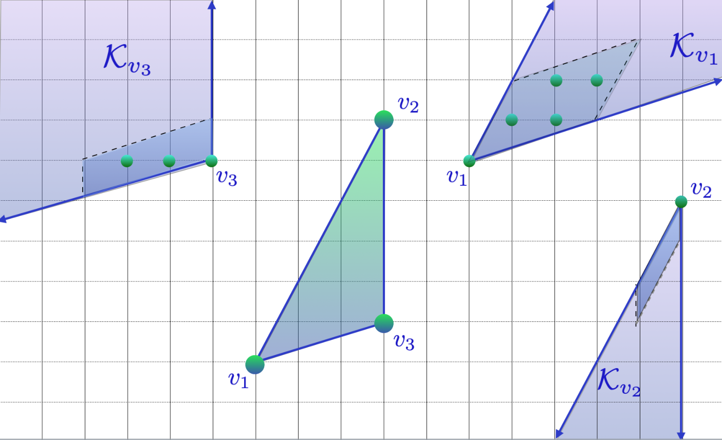
10.3 Examples, examples, examples
Example 10.3.
Here we will compute the integer point transform of the triangle defined by the convex hull of the points , as shown in Figure 10.2. We first compute the integer point transforms of all of its tangent cones. For the vertex , we already computed the integer point transform of its tangent cone in the previous example.
For the vertex , we notice that its vertex tangent cone is a unimodular cone, because . Its integer point transform is:
Equivalently, using the notation from Example 10.4 above,
For vertex , the computation is similar to vertex tangent cone , and we have:
Finally, putting all of the three vertex tangent cone contributions together, Theorem 10.1 gives us:
Example 10.4.
We work out the integer point transform of the cone
Drawn in the figures below. We note that here , and that there are indeed integer points in , its half-open fundamental parallelepiped.


We may ‘divide and conquer’ the integer point transform , by breaking it up into infinite series, one for each integer point in , as follows:
where
and similarly we have
and finally
To summarize, we have the following expression:
Equivalently, using our multinomial notation , we have
10.4 Integer point transforms of rational cones are rational functions
The Examples 10.3 and 10.4 above suggest a general pattern, namely that integer point transforms are always rational functions, and that their numerators are polynomials that encode the integer points inside a fundamental parallelepiped that sits at the vertex of each vertex tangent cone. The proof of this general fact will be fairly easy - we only need to put several geometric series together, as in Figure 10.4. Now that we’ve seen some examples, we can prove things in general.
First, given any -dimensional simplicial rational cone , with integer edge vectors , and apex , we define the fundamental parallelepiped of by:
| (10.11) |
a half-open, integer parallelepiped. In the same way that we’ve encoded integer points in polytopes using , we can encode the integer points in by defining
For a rational simplicial cone , it turns out that its integer point transform
has a pretty structure theorem - it is a rational function of the variables , as follows.
Theorem 10.2.
Given a -dimensional simplicial cone , with apex , and with linearly independent integer edge vectors . Then:
| (10.12) |
Proof.
We claim that we can parametrize all of the integer points in the cone precisely by
| (10.13) |
To prove (10.13), we begin by writing each , by definition of the cone , as follows:
with the . This representation of is unique, because is a basis for . Now we use the fact that each , where is the fractional part of :
where we’ve defined . We now notice that , and in fact , because .
Since tiles the cone precisely by the translation vectors , we see that the set of all integer points in is precisely the disjoint union of the sets
| (10.14) |
(which we may think of as ‘multidimensional arithmetic progressions’) , as varies over the integer points of . Finally, we expand each denominator in the following rational function as a geometric series to get:
Multiplying out all of these geometric series together, we see that the exponents look precisely like the points in (10.14). ∎
Notes
- 1.
In the development of our text so far, we’ve observed that the discrete version of Brion’s theorem (Theorem 10.1) followed from the continuous version of Brion’s theorem (Theorem 8.2). The tool we used in order to discretize Theorem 8.2 was the Poisson summation formula. By contrast, the ideas in our previous book [24] developed in exactly the opposite direction: in that context we first proved the discrete Brion theorem, and then derived the continuous version from it.
Exercises
10.1.
Suppose that is a unimodular polytope, with vertex set . Using Theorem 10.1, show that its integer point transform is equal to:
| (10.15) |
10.2.
Fix a positive integer , and let be the -dimensional triangle whose vertices are given by , and . First compute the integer point transforms for its three vertex tangent cones, and then compute the integer point transform .
10.3.
Given a positive integer , find the integer point transform for the -dimensional cone whose edge vectors are
10.4.
More generally, given any coprime positive integer , find the integer point transform for the -dimensional cone whose edge vectors are
10.5.
Let be the -dimensional polytope.
- 1.
Prove the following inequality for the integer point transform:
for all .
- 2.
Is it true that for all , we have
10.6.
Let be the -dimensional simplex whose vertices are given by , and . Compute the integer point transforms of its four vertex tangent cones , and then compute the integer point transform of .
10.7.
Suppose we are given a -dimensional simplicial integer cone , together with its dual cone . Is there a simple relationship between the integer point transforms and in dimension ?
Notes. For this problem, it’s worth thinking about the relationship between the edge vectors of the fundamental parallelepipeds for and .
Chapter 11 Counting integer points in polytopes - the Ehrhart theory
“How wonderful that we have met with a paradox. Now we have some hope of making progress. ”
-- Niels Bohr
![[Uncaptioned image]](2104.06407v7/DiscreteArea.png)
(Under construction)
11.1 Intuition
A basic question in discrete geometry is “how do we discretize volume?”
One method of discretizing the volume of is to count the number of integer points in . Even in , this question may be highly non-trivial, depending on the arithmetic properties of the vertices of . Ehrhart first considered integer dilations of a fixed, integer polytope , and studied the integer point enumerator:
| (11.1) |
where is the ’th dilate of , and is a positive integer. Ehrhart showed that is a polynomial in the positive integer parameter , known as the Ehrhart polynomial of .
Viewed from the lens of Fourier analysis, Ehrhart polynomials may be computed by ‘averaging’ the Fourier transform of a polytope over the full integer lattice:
| (11.2) | ||||
| (11.3) | ||||
| (11.4) |
where we’ve used Poisson summation in the third equality. But because we may not use indicator functions directly in Poisson summation, some care is required and the process of smoothing may be applied to .

As we’ve just seen in (11.2), the integer point enumerator , expanded using Poisson summation, has the primary term . We recall the definition of the volume of , and of the Riemann integral:
More generally, given a function , we may sum the values of at all integer points and observe how close this sum gets to the integral of over . This approach is known as Euler-Maclaurin summation over polytopes, and is a current and exciting topic of a growing literature (see Note 10 below). In this chapter we’ll also compare the above combinatorial method of discretizing volume, namely (11.1), to our previous discrete volumes of Chapter 9, which used solid angles.
11.2 Computing integer points in polytopes via the discrete Brion Theorem
Example 11.1.
Probably the simplest example in is the unit square . As Figure 11.1 suggests, the -dilate here contains points of the integer lattice . Here it was easy to conclude that was a polynomial function of , but by a small miracle of nature a similar phenomenon occurs for all integer polytopes in .
If all of the vertices of have integer coordinates, we call an integer polytope. On the other hand, if all of the vertices of a polytope have rational coordinates, we call a rational polytope.
Let be a rational, -dimensional polytope, and let be the number of its vertices. For each vertex of , we consider the vertex tangent cone of . Once we dilate by , each vertex of gets dilated to become , and so each of the vertex tangent cones of simply get shifted to the corresponding vertex tangent cone of . Using the discrete Brion theorem (Theorem 10.1), we have
| (11.5) |
for all , where is the hyperplane arrangement defined by the (removable) singularities of all of the transforms . To simplify notation, we have absorbed the constant into the complex vector by replacing by . We recall that we rewrote (11.5) by using the notation:
| (11.6) |
And now we notice that when , the left-hand-side gives us precisely
which is good news - it is the Ehrhart polynomial , by definition. The bad news is that is a singularity of the right-hand-side of (11.6). But then again, there is still more good news - we already saw in the previous chapter that it is a removable singularity. So we may let , and discover what happens.
Example 11.2.
Let’s see by example how we can start with the discrete integer point transform, and end up with an Ehrhart polynomial. We will find a formula for the Ehrhart polynomial of the standard triangle, continuing Example 10.2. It turns out that the method we use in this example is universal - it can always be used to find the Ehrhart polynomial of any rational polytope. We will formalize this method in the ensuing sections.
In this example we are lucky in that we may use brute-force to compute it, since the number of integer points in the -dilate of may be computed along the diagonals:
Now we can confirm this lucky answer with our brand new machine, as follows. Using (11.5), and the formulation (10.10) from Example 10.2., we have the integer point transform for the dilates of :
| (11.7) | ||||
| (11.8) | ||||
| (11.9) |
where we have defined by the last equality. We can let along almost any direction, but it turns out that we can simplify our computations by taking advantage of the symmetry of this polytope, so we will pick , which will simplify our computations (see Note 8). Here is our plan:
- 1.
We pick .
- 2.
We expand all three meromorphic functions in terms of their Laurent series in , giving us Bernoulli numbers.
- 3.
Finally, we let , to retrieve the constant term (which will be a polynomial function of ) of the resulting Laurent series.
To expand in their Laurent series, we recall the definition 3.24 of the Bernoulli numbers in terms of their generating function, namely :
Similarly, we have
Now, by symmetry we see that , so that by (11.9) and the latter expansions, we finally have:
Letting in the latter computation, we retrieve the (Ehrhart) polynomial:
as desired.
11.3 The Ehrhart polynomial of an integer polytope, and the Ehrhart quasi-polynomial of a rational polytope

Eugene Ehrhart initiated a systematic study of the integer point enumerator
for an integer polytope , which Ehrhart proved was always a polynomial function of the positive integer dilation parameter . Ehrhart also proved that for a rational polytope , the integer point enumerator is a quasi-polynomial in the positive integer parameter , which means by definition that
| (11.10) |
where each is a periodic function of .
The study of Ehrhart polynomials and Ehrhart quasi-polynomials has enjoyed a renaissance in recent years ([17], [24]), and has some suprising connections to many branches of science, and even to voting theory, for example.
Theorem 11.1 (Ehrhart).
For an integer polytope
, its discrete volume
is a polynomial functions of , for all positive integer values of the dilation parameter . Moreover, we have
| (11.11) |
Ehrhart’s Theorem 11.1 has an extension to rational polytopes, as follows. We will derive the more general Theorem 11.2 of Ehrhart, by using the discrete Brion Theorem 10.1.
Theorem 11.2 (Ehrhart).
For a rational polytope
, its discrete volume
is a quasi-polynomial function of , for all positive integer values of the dilation parameter .
In particular, we have
| (11.12) |
where each quasi-coefficient is a periodic function of .

Proof.
To begin, suppose that the least common denominator of the coordinates of all the rational vertices of . We need to show that, for each fixed , the integer point enumerator is a polynomial in the parameter . By definition of a quasi-polynomial, this will prove that is a quasi-polynomial in . In other words, we restrict attention to each fixed arithmetic progression of dilations in . Now, from the discrete Brion Theorem 10.1, we know that
| (11.13) |
and we also know the elementary relation
So we’d like to let on both sides of Brion’s discrete identity (11.13):
| (11.14) |
The bad news is that the right-hand-side of (11.13) introduces local singularities in the denominators of each rational-exponential function
But there is good news too! These singularities must be removable singularities. The reason is easy - is a finite sum of exponentials (by compactness of ), and is therefore an analytic function of , so any singularities on the right-hand side of (11.13) must be removable singularities. To proceed further, we’ll begin by writing each vertex tangent cone in terms of its vertex , and edge vectors :
Now we consider the dilates of a bit more carefully, and we will use the fact that the edge vectors of any dilate of a vertex tangent cone remain invariant, as in Figure 11.3:
Case . Suppose . Then:
The salient feature of this computation is that is an integer vector, by definition of . This implies that
Summarizing, (11.14) gives us:
and giving a common denominator to all of the rational functions (of ) , we may apply L’Hospital’s rule a finite number of times. Because the integer variable only appears in the exponents , we see that each time we apply L’Hospital, an extra factor of comes down, giving us a polynomial function of .
Case . Suppose . Here the situation is slightly easier: , so
which is an integer cone because is an integer vector, and is an integer cone with apex at the origin. Similarly to the computation above, we have
and the remaining steps are identital to Case . ∎
We note that for an integer polytope , the same proof gives us Theorem 11.1, namely that is a polynomial for positive integer dilations ; here we just need Case , with , so that and .
We emphasize again that one of the important steps in the latter computation was the fact that in both cases of the proof above, was an integer vector, allowing us to rewrite the integer point transform of the cone in a simpler way. As a first application of Theorem 11.1, we show that the discrete volume of a (half-open) parallelepiped has a particularly elegant and useful form.
Lemma 11.1.
Let be any half-open integer parallelepiped in , defined by
where are linearly independent. Then:
| (11.15) |
and for each positive integer , we also have
Proof.
We can tile by using translates of , because is half-open. Therefore
and by definition . On the other hand, we also know by Ehrhart’s Theorem 11.1 that is a polynomial for integer values of , whose leading coefficient is . Since for all positive integer values of , we conclude that
∎
11.4 The Ehrhart series
Given an integer -dimensional polytope , we now recall one of Ehrhart’s tricks, which entails building a -dimensional integer cone from all of the integer dilates of .
We first place a copy of in the hyperplane, so that this copy of has the form . If are the vertices of , we define a -dimensional cone called Cone(), by using the edge vectors . By construction, Cone() has apex at the origin, and is a pointed cone in . Moreover, Cone() is naturally built up from all of the simultaneous dilations of , appearing as slices of Cone() parallel to the hyperplane, as in Figure 11.4. Cone() is sometimes called the cone over (and this process is sometimes called homogenizing a polytope).

Our next goal is to write down the integer point transform of Cone(), so we first parametrize all of its integer points:
with the convention that when , we define (the zeroth dilate) to be the origin. We recall that the integer point transform of any cone is defined by , but we will now specialize to , and we also define to get the following special case of the integer point transform:
The latter series is a generating function for the Ehrhart polynomial of , evaluated at all nonnegative integers, and it is by definition the Ehrhart series of :
One of the first and most famous Ehrhart-type theorems, discovered and proved by Richard Stanley [229], is the following characterization for the Ehrhart series of integer polytopes.
Theorem 11.3 (Stanley).
Suppose that is a -dimensional integer polytope. Then its Ehrhart series is given by
and the coefficients are all nonnegative integers.
(For a proof see, for example, [24] Theorem )
11.5 Families of Ehrhart polynomials
Example 11.3 (The unit cube).
The simplest family consists of the -dimensional unit cube in , defined by . This family extends Example 11.1. Here, the -dilate has integer points, giving us the polynomial
for each positive integer value of .
Example 11.4 (The standard simplex).
For the standard simplex , we consider its -dilate, given by
We can quickly compute its Ehrhart polynomial by using combinatorics. By definition, we need to find the number of nonnegative integer solutions to
which is equal to , for each fixed positive integer . We can introduce a ‘slack variable’ , to transform the latter inequality to an equality: , where . By a very classical and pretty argument, (involving placing balls into urns that are separated by walls) this number is equal to (Exercise 11.17). So we find that
| (11.16) |
a degree polynomial, valid for all positive integers .
What about the interior of ? Here we need to find the number of positive integer solutions to , for each positive integer . It turns out that by a very similar argument as above (Exercise 11.18), the number of positive integer solutions is . So is it really true that
Let’s compute, substituting for in (11.16) to get:
confirming that Ehrhart reciprocity works here as well.
Example 11.5 (A Pyramid).
Example 11.6 (Zonotopes).
Example 11.7 (The crosspolytope).
Example 11.8 (The permutohedron).
We consider the vector , together with all of the vectors whose coordinates are permutations of the coordinates of , and we take their convex hull. In other words, if we let be the symmetric group, then the Permutohedron is defined by the convex hull
where runs over all permutations in . It may be somewhat surprising to realize that the coefficients of the Ehrhart polynomial of count forests in graph theory. To recall the definitions, a tree is a connected graph (undirected) that does not contain any cycles. A forest is a disjoint union of trees.
Theorem 11.4.
If is the permutohedron, then
where is the number of forests with edges, on the graph whose nodes are labelled .
For example, when , the Permutohedron is the convex hull of the six integer points:
which is a hexagon sitting in .
Add: forests with edges on a graph with nodes are pictured in Figure …………… ( or - ADD PICTURE HERE).
Question 25.
Is it possible to somehow classify completely the vectors that occur as a -vector for some integer polytope ?
11.6 Unimodular polytopes
We recall that the standard basis vectors of are defined by the set , where is the unit vector pointing in the direction. A -dimensional integer simplex is called a unimodular simplex if is the unimodular image of the standard simplex , which we recall is the convex hull of the points .


Example 11.9.
Let , their convex hull. Then is a unimodular simplex, because the unimodular matrix maps the standard simplex to .
It is not difficult to show that each of the tangent cones of a unimodular simplex possesses edge vectors that form a lattice basis for . Thus, it is natural to define a unimodular cone as a simplicial cone, possessing the additional property that its edge vectors form a lattice basis for .
Example 11.10.
We consider the polygon in Figure 11.5. An easy verification shows that each of its vertex tangent cones is unimodular. For example, focusing on the vertex , we see from Figure 11.6, that its vertex tangent cone is . is a unimodular cone, because the matrix formed by the its two edges and is a unimodular matrix.
More generally, a simple, integer polytope is called a unimodular polytope if each of its vertex tangent cones is a unimodular cone. Unimodular polytopes are the first testing ground for many conjectures in discrete geometry and number theory. Indeed, we will see later that the number of integer points in a unimodular polytope, namely , admits a simple and computable formula, if we are given the local tangent cone information at each vertex. By contrast, it is in general thought to be quite difficult to compute the number of integer points , even for (general) simple polytopes, a problem that belongs to the NP-hard class of problems (if the dimension is not fixed). The following fact, however, is elementary.
Lemma 11.2.
Suppose we have two integer polytopes , which are unimodular images of each other:
for some unimodular matrix . Then , for all .
Next, we can generalize Exercise 5.7, regarding primitive triangles, to all integer simplices that intersect that integer lattice only in their vertices, as follows.
Theorem 11.5.
Suppose that is a -dimensional integer simplex. Then the following properties are equivalent:
- 1.
Aside from its integer vertices, has no other integer points in its interior, or on its boundary.
- 2.
.
- 3.
is a unimodular simplex.
11.7 More examples of rational polytopes and quasi-polynomials
The following properties for the floor function, the ceiling function, and the fractional part function are often useful. It’s convenient to include the following indicator function, for the full set of integers, as well:
the indicator function for . For all , we have:
- 1.
- 2.
- 3.
- 4.
, for all .
- 5.
Let . Then .
(Exercise 11.15)
Example 11.11.
Let’s find the integer point enumerator of the rational line segment . Proceeding by brute-force, for we have
| (11.17) | ||||
| (11.18) | ||||
| (11.19) | ||||
| (11.20) |
a periodic function on with period . Here we used property 1 in the third equality. In fact, here we may let be any positive real number, and we still obtain the same answer, in this -dimensional case.
Now we will compare this to a new computation, but this time from the perspective of the vertex tangent cones. For the cone , we can parametrize the integer points in this cone by , so that
For the cone , we can parametrize the integer points in this cone by , so that
So by the discrete Brion Theorem (which is here essentially a finite geometric sum), we get:
as , recovering the same answer 11.17 above.
Example 11.12.
Let’s find the integer point enumerator of the rational triangle
First we will proceed by brute-force (which does not always work well), and then we will use the machinery of (11.5).
For the brute-force method, we need to consider separately the even integer dilates and the odd integer dilates. Letting be a positive even integer, it’s clear geometrically that
On the other hand, if , then we notice that we never have an integer point on the diagonal face of , so that in this case we get:
Alternatively, we may also rederive the same answer by using the Brion identity (11.5). We can proceed as in Example 11.2. The only difference now is that the vertex tangent cones have rational apices. So although we may still use the same edge vectors to parametrize the integer points in , we now have a new problem: the rational vertex . But in any case, we get: . We invite the reader to complete this alternate derivation of the Ehrhart quasi-polynomial in this case.

11.8 Ehrhart reciprocity
There is a wonderful, and somewhat mysterious, relation between the Ehrhart polynomial of the (closed) polytope , and the Ehrhart polynomial of its interior, called . We recall our convention that all polytopes are, by definition, closed polytopes. We first compute , for positive integers , and once we have this polynomial in , we formally replace by . So by definition, we form algebraically, and then embark on a search for its new combinatorial meaning.
Theorem 11.6 (Ehrhart reciprocity).
Given a -dimensional rational polytope , let the integer point enumerator of its interior. Then
| (11.21) |
for all .
Offhand, this reciprocity law seems like ‘a kind of magic’, and indeed Ehrhart reciprocity is one of the most elegant geometric inclusion-exclusion principles we have. Some examples are in order.
Example 11.13.
For the unit cube , we can easily compute from first principles . For the open cube (the interior of ), we can also easily compute
using our known polynomial .
A very common question in integer linear programming, as well as convex geometry, is:
Question 26.
Given an integer polytope , does it contain an integer point in its interior?
As a fun and rapid consequence of Ehrhart reciprocity, we can give approach Question 26 in terms of the coefficients of the Ehrhart polynomial.
Lemma 11.3.
Let be an integer polytope, and let its Ehrhart polynomial be
. Then
with equality does not contain an integer point in its interior.
Proof.
By Ehrhart reciprocity, namely Theorem 11.6, we have
But we also have , with equality if and only if there are no integer points in the interior of . ∎
As of this writing, the true complexity of finding even one integer point inside a given integer polytope is not known, but this problem is known to be NP-hard. Theorem 11.6 also suggests that computing coefficients of Ehrhart polynomials appears to be hard in general.
11.9 The Möbius inversion formula for the face poset
Given a polytope , the collection of all faces of - including the empty set and itself - is ordered by inclusion. This ordering forms a partially ordered set, and is called the face poset. There is a particularly useful inversion formula on this face poset.
Theorem 11.7 (Möbius inversion formula for the face poset).
Given any function , we may define a sum over the face poset of :
| (11.22) |
We then have the following inversion formula:
| (11.23) |
To prove (again) that for positive integer values of , the angle polynomial is indeed a polynomial in , we may use the following useful little relation between solid angle sums and integer point sums. We recall that for any polytope , the integer point enumerator for the relative interior of was defined by .
For each face , we define the -dimensional solid angle of the face by picking any point inside the relative interior of and denoting
Theorem 11.8.
Let be a -dimensional polytope in . Then we have
| (11.24) |
Proof.
The polytope is the disjoint union of its relatively open faces , and similarly the dilated polytope is the disjoint union of its relatively open faces . We therefore have:
But by definition each is constant on the relatively open face of , and we denoted this constant by . Altogether, we have:
∎
Theorem 11.9.
Given an integer polytope , the discrete volume is a polynomial in , for integer values of the dilation parameter .
Proof.
We may apply Theorem 11.7 to invert the relationship in Theorem 11.8 between solid angle sums and local Ehrhart polynomials, to get the following consequence of the Möbius inversion formula.
Corollary 11.1.
Let be a -dimensional polytope. Then we have
| (11.25) |
Proof.

Example 11.14.
Let’s work out a special case of Corollary 11.1, in , for the triangle appearing in Figure 11.8, with . has vertices , and edges .
We have to compute for each face . At the vertices, we have , , and . For the edges of , we have:
Finally, for itself, we have
Putting everything together, we have:
the number of interior integer points in .
Finally, we mention a fascinating open problem by Ehrhart.
Question 27 (Ehrhart, 1964).
Let be a d-dimensional convex body with the origin as its barycenter. If the origin is the only interior integer point in , then
and futhermore the equality holds if and only if is unimodularly equivalent to , where is the -dimensional standard simplex.
Notes
- 1.
Ehrhart theory has a fascinating history, commencing with the fundamental work of Ehrhart [74], [75], [76], [77], in the 1960’s. Danilov [62] made a strong contribution to the field, but after that the field of Ehrhart theory lay more-or-less dormant, until it was rekindled by Jamie Pommersheim in 1993 [185], giving it strong connections to Toric varieties. Using the Todd operators to discretize certain volume deformations of polytopes, Khovanskii and Pukhlikov discovered a wonderful result that helped develop the theory further (see Theorem 12.6 of [24]). In 1993, Alexander Barvinok [14] gave the first polynomial-time algorithm for counting integer points in polytopes in fixed dimension.
In recent years, Ehrhart theory has enjoyed an enthusiastic renaissance (for example, the books [17], [24], [88]). Early connections between Ehrhart theory and Fourier analysis appeared in [69] and [47]. For more relations with combinatorics, the reader may enjoy reading Chapter of the classic book “Enumerative Combinatorics”, [228] by Richard Stanley.
- 2.
- 3.
Regarding the computational complexity of counting integer points in polytopes, Alexander Barvinok settled the problem in [14] by showing that for a fixed dimension , there is a polynomial-time algorithm, as a function of the ‘bit capacity’ of any given rational polytope , for counting the number of integer points in .
- 4.
It is also true that for integer polytopes which are not necessarily convex (for example simplicial complexes), the integer point enumerator makes sense as well. In this more general context, the constant term of the corresponding integer point enumerator equals the (reduced) Euler characteristic of the simplicial complex.
- 5.
For more information about the rapidly expanding field of Euler-MacLaurin summation over polytopes, a brief (and by no means complete) list of paper in this direction consists of the work by Berligne and Vergne [22], Baldoni, Berline, and Vergne [8], Garoufalidis and Pommersheim [89], Brandolini, Colzani, Travaglini, and Robins [45], Karshon, Sternberg, and Weitsman ([124], [125]), and very recently Fischer and Pommersheim [83].
- 6.
There are some fascinating relations between an integer polytope and its polar polytope . In particular, let be an integer polygon (convex) whose only interior integer point is the origin. Such polygons are called reflexive polygons, and up to unimodular transformations there are only a finite number of them in each dimension. If we let be the number of integer points on the boundary of , then Bjorn Poonen and Fernando Villegas proved [186] that
One way to see why we get the number “12” is to consider Bernoulli numbers and Dedekind sums, but in [186] the authors give 4 different proofs, including Toric varieties and modular forms.
- 7.
The book [21] by Matthias Beck and Raman Sanyal covers many classical instances of combinatorial reciprocity that appear in combinatorial geometry, including the reciprocity for the order polynomial of a poset.
- 8.
The trick used in Example 11.2 of picking the particular vector , which turns out to simplify the computations a lot, is due to Michel Faleiros.
- 9.
There is a fascinating theory that offers an abstract extension of many of the ideas in this chapter, called valuation theory. The author may wish to consult the excellent introduction to this field, by Katharina Jochemko [120]. Allowing the empty set to be included in the collection of all convex bodies, we may define a valuation as any mapping
where is an abelian group (think of ), with the following properties:
for all such that and are also convex bodies. The volume of a convex body, as well as the Ehrhart polynomial of an integer polytope, are just two examples of valuations. Two of the founders of this theory are Peter McMullen [162] and Jim Lawrence [145].
- 10.
In a future version of this book, we will also delve into Dedekind sums, which arise very naturally when considering the Fourier series of certain rational-exponential functions. To define a general version of these sums, let be a -dimensional lattice in , let be linearly independent vectors from , and let be a matrix with the ’s as columns. For any -tuple of positive integers , define . Then, for all , a lattice Dedekind sum is defined by
(11.28) Gunnells and Sczech [100] have an interesting reduction theorem for these sums, giving a polynomial-time complexity algorithm for them, for fixed dimension .
Exercises
If there is a problem you can’t solve, then there is an easier problem you can’t solve: find it.
– George Polya
11.1.
In , consider the -dimensional polytope , for any .
- 1.
Show that the Ehrhart polynomial of is .
- 2.
Find the Ehrhart quasi-polynomial for the rational segment .
11.2.
Fix positive integers . Working in , show that the closed line segment , whose vertices are the origin and , contains exactly integer points of . Conclude that we have the lower-dimensional Ehrhart polynomial .
11.3.
We recall that the -dimensional cross-polytope was defined by
For , find the Ehrhart polynomial .
11.4.
11.5.
Let , and consider the cross-polytope . Find the Ehrhart quasi-polynomial for the rational polygon .
11.6.
Suppose is the standard simplex in . Show that the first dilations of do not contain any integer points in their interior:
for . In other words, show that . Conclude that the same statement is true for any unimodular simplex.
11.7.
Here we show that the Bernoulli polynomial , is essentially equal to the Ehrhart polynomial for the “Pyramid over a cube” (as defined in Exercise 8.6). We recall the definition: let be the -dimensional cube, considered as a subset of , and let be the unit vector pointing in the -direction. Now we define , a pyramid over the unit cube. Show that its Ehrhart polynomial is
for .
11.8.
For any integer -dimensional (convex) polytope , show that
| (11.29) |
which can be thought of as yet another generalization of Pick’s formula to .
Note. Using iterations of the forward difference operator
the latter identity may be thought of a discrete analogue of the ’th derivative of the Ehrhart polynomial. This idea in fact gives another method of proving (11.29).
11.9.
Show that Pick’s formula is the special case of Exercise 11.8 when the dimension . That is, given an integer polygon , we have
where is the number of interior integer points in , and B is the number of boundary integer points of .
11.10.
Fix . Show that the convolution of the indicator function with the heat kernel , as in equation (9.11), is a Schwartz function (of ).
11.11.
Show that any unimodular triangle has area equal to .
11.12.
Show that the Ehrhart polynomial of the standard simplex is
11.13.
Consulting Figure 11.5:
- 1.
Find the integer point transform of the unimodular polygon in the Figure.
- 2.
Find the Ehrhart polynomial of the integer polygon from part (a).
11.14.
Show that (9.5) is equivalent to the following definition, using balls instead of spheres. Recall that the unit ball in is define by , and similarly the ball of radius , centered at , is denoted by . Show that for all sufficiently small , we have
11.15.
Here we gain some practice with ‘floors’, ‘ceilings’, and ‘fractional parts’. First, we recall that by definition, the fractional part of any real number is . Next, we recall the indicator function of , defined by:
Show that:
- 1.
- 2.
- 3.
- 4.
, for all .
- 5.
Let . Then .
11.16.
Show that for , we have:
| (11.30) |
where we recall the definition of the first periodic Bernoulli polynomial .
11.17.
Show that the number of nonnegative integer solutions to
with , equals .
11.18.
Show that for each positive integer , the number of positive integer solutions to is equal to .
11.19.
We define the rational triangle whose vertices are , where is a fixed integer. Prove that the Ehrhart quasi-polynomial is in this case
for all .
Notes. So we see here a phenomenon known as ‘period collapse’, where we expect a quasi-polynomial behavior, with some nontrivial period, but in fact we observe a strict polynomial.
11.20.
Here we show that the Ehrhart polymomial remains invariant under the full unimodular group . In particular, recalling definition 6.3, of a unimodular matrix, show that:
- 1.
Every element of acts on the integer lattice bijectively.
- 2.
Let be an integral polytope, and let , where . In other words, and are unimodular images of each other, by definition. Prove that
for all .
- 3.
Is the converse of part 2 true? In other words, given integer polytopes , suppose that , for all positive integers . Does it necessarily follow that , for some unimodular matrix ?
11.21.
Suppose we are given a general lattice for some invertible matrix . Here we extend the notion of the Ehrhart polynomial, so that we are counting elements of :
So by definition . show that:
- 1.
.
- 2.
.
Chapter 12 The Fourier transform of a polytope via its hyperplane description:
Stokes’ Theorem
“Like a zen koan, Stokes’ Theorem tells us that in the end, what happens on the outside is purely a function of the change within.”
–Keenan Crane

(Under construction)
12.1 Intuition
The divergence theorem, which is a special case of Stokes’ more general theorem, is a multi-dimensional version of “integration by parts”, a powerful tool from the -dimensional calculus. We’ll apply the divergence theorem to a polytope, to obtain a combinatorial version of the divergence theorem. This discrete version of the divergence theorem will allow us to transfer some of the complexity of computing the Fourier transform of a polytope to the complexity of computing corresponding Fourier transforms of its facets. This kind of game can be iterated, yielding interesting geometric identities and results for polytopes, as well as for discrete volumes of polytopes.
In the process, we also obtain another useful way to compute the Fourier transform of a polytope in its own right.
12.2 The divergence theorem, and a combinatorial
divergence theorem for polytopes
To warm up, we recall the divergence theorem, with some initial examples. A vector field on Euclidean space is a function that assigns to each point in another vector in , which we will denote by
If is a continuous (respectively, smooth) function, we say that is a continuous vector field (respectively, smooth vector field). If all of the coordinate functions are real-valued functions, we say that we have a real vector field.
We define the divergence of at each by
assuming that is a smooth (or at least once-differentiable) vector field. This divergence of is a measure of the local change (sink versus source) of the vector field at each point . Given a surface , and an outward pointing unit normal vector , defined at each point , we also define the flux of the vector field across the surface by
where denotes the Lebesgue measure of the surface , and where the dot product is the usual inner product . We will apply the divergence theorem (which is technically a special case of Stokes’ Theorem) to a polytope , and its -dimensional bounding surface . Intuitively, the divergence theorem tells us that the total divergence of a vector field inside a manifold is equal to the total flux of across its boundary.
Theorem 12.1 (The Divergence Theorem).
Let be a piecewise smooth manifold, and let be a smooth vector field. Then
| (12.1) |
Example 12.1.
Let be a -dimensional polytope, containing the origin, with defining facets . Define the real vector field
for all . First, we can easily compute here the divergence of , which turns out to be constant:
If we fix any facet of then, due to the piecewise linear structure of the polytope, every point has the same constant outward pointing normal vector to , which we call . Computing first the left-hand-side of the divergence theorem, we see that
| (12.2) |
Computing now the right-hand-side of the divergence theorem, we get
Now it’s easy to see that the inner product is constant on each facet , namely it is the distance from the origin to (Exercise 12.4), denoted by . So we now have
so that altogether we the following conclusion from the divergence theorem:
| (12.3) |
known as “the pyramid formula” for a polytope, a classical result in Geometry, which also has a very easy geometrical proof (Exercise 12.2).
Example 12.2.
Let be a -dimensional polytope with defining facets , and outward pointing unit vectors . We fix any constant vector , and we consider the constant vector field
defined for all . Here the divergence of is , because is constant, and so the left-hand-side of Theorem 12.1 gives us
Altogether, the divergence theorem gives us:
and because this holds for any constant vector , we can conclude that
| (12.4) |
Identity (12.4) is widely known as the Minkowski relation for polytopes. There is a marvelous converse to the latter relation, given by Minkowski as well, for any convex polytope (See Theorem 12.8).
Now we fix , and we want to see how to apply the divergence theorem to the vector-field
| (12.5) |
Taking the divergence of the vector field , we have:
So by the divergence theorem we have
| (12.6) |
where is the outward-pointing unit normal vector at each point . When is a polytope, these arguments quickly give the following conclusion.
Theorem 12.2.
Given any -dimensional polytope , with outward pointing normal vector to each facet of , its Fourier transform has the form
| (12.7) |
for all nonzero . Here the integral that defines each is taken with respect to Lebesgue measure that matches the dimension of the facet .
Proof.
where in the third equality we used the fact that the boundary of a polytope is a finite union of -dimensional polytopes (its facets), and hence , a sum of integrals over the facets of . ∎
This result allows us to reduce the Fourier transform of to a finite sum of Fourier transforms of the facets of . This process can clearly be iterated, until we arrive at the vertices of . But we will need a few book-keeping devices first.
To simplify the notation that will follow, we can also the Iverson bracket notation, defined as follows. Suppose we have any boolean property , where ; that is, is either true or false. Then the Iverson bracket is defined by:
| (12.8) |
Now we may rewrite the identity of Theorem 12.2 as follows:
| (12.9) |
Later, after Theorem 12.3 below, we will return to the Iverson bracket, and be able to use it efficiently. To proceed further, we need to define the affine span of a face of :
| (12.10) |

In other words, we may think of the affine span of a face of as follows. We first translate by any element . So this translate, call if , contains the origin. Then we take all real linear combinations of points of , obtaining a vector subspace of , which we call the linear span of . Another way to describe the linear span of a face of is:
Finally, we may translate this subspace back using the same translation vector , to obtain (see Figure 12.2).
Example 12.3.
The affine span of two distinct points in is the unique line in passing through them. The affine span of three points in is the unique -dimensional plane passing through them. The affine span of a -dimensional polytope is a translate of a -dimensional vector subspace of . Finally, the affine span of a whole -dimensional polytope is all of .
In formalizing (12.7) further, we will require the notion of the projection of any point onto the linear span of any face , which we abbreviate by :
| (12.11) |
(see Figure 12.2) We will also need the following elementary fact. Let be any -dimensional polytope in , and fix the outward-pointing unit normal to , calling it . It is straightforward to show that if we take any point , then is the distance from the origin to . Therefore, if , then a straightforward computation shows that (Exercise 12.4).
12.3 A combinatorial divergence theorem
We’re now ready to extend (12.7) to polytopes whose dimension is lower than the ambient dimension, as follows.
Theorem 12.3 (Combinatorial Divergence Theorem).
Let be a polytope in , where . For each facet , we let be the unit normal vector to , with respect to . Then for each , we have:
- 1.
If , then
(12.12) - 2.
If , then
(12.13)
We notice that, as before, we are getting rational-exponential functions for the Fourier transform of a polytope. But Theorem 12.3 gives us the extra freedom to begin with a lower-dimensional polytope , and then find its Fourier transform in terms of its facets.
We are now set up to iterate this process, defined by Theorem 12.3, reapplying it to each facet . Let’s use the Iverson bracket, defined in (12.8), and apply the combinatorial divergence Theorem 12.3 to twice:
It is an easy fact that the product of two Iverson brackets is the Iverson bracket of their intersection: (Exercise 12.11). Hence, if we define
Then we see that , and we can rewrite the latter identity as
In order to keep track of the iteration process, we will introduce another book-keeping device. The face poset of a polytope is defined to be the partially ordered set (poset) of all faces of , ordered by inclusion, including and the empty set.
Example 12.4.
Consider a -dimensional polytope that is a triangle. We have the following picture for the face poset of , as in Figure 12.3. It turns out that if we consider a -simplex , then its face poset has the structure of a “Boolean poset” (which is isomorphic to the edge graph of a -dimensional cube).

We only have to consider rooted chains in the face poset , which means chains whose root is . The only appearance of non-rooted chains are in the following definition. If is a facet of , we attach the following weight to any (local) chain , of length , in the face poset of :
| (12.14) |
Note that these weights are functions of rather than constants. Moreover, they are all homogeneous of degree . Let be any rooted chain in , given by
so that by definition . We define the admissible set of the rooted chain to be the set of all vectors that are orthogonal to the linear span of but not orthogonal to the linear span of . In other words,
Finally, we define the following weights associated to any such rooted chain :

- 1.
The rational weight is defined to be the product of weights associated to all the rooted chains of length , times the Hausdorff volume of (the last node of the chain ). It is clear from this definition that is a homogenous rational function of .
- 2.
The exponential weight is defined to be the evaluation of at any point on the face :
(12.15) for any . We note that the inner product does not depend on the position of .
- 3.
The total weight of a rooted chain is defined to be the rational-exponential function
(12.16) where is the indicator function of the admissible set of .
By repeated applications of the combinatorial divergence Theorem 12.3, we arrive at a description of the Fourier transform of as the sum of weights of all the rooted chains of the face poset , as follows.
Theorem 12.4.
| (12.17) |
valid for any fixed .
For a detailed proof of Theorem 12.4, see [70]. Using this explicit description of the Fourier transform of a polytope, we will see an application of it in the following section, for the coefficients of Macdonald’s angle quasi-polynomial. In the process, equation (12.17), which gives an explicit description of the Fourier transform of a polytope, using the facets of as well as lower-dimensional faces of , will become even more explicit with some examples.
12.4 Generic frequencies versus special frequencies
Given a polytope , we call a vector a generic frequency (relative to ) if is not orthogonal to any face of . All other are orthogonal to some face of , and are called special frequencies.
We see from Theorem 12.4 that for a generic frequency , we have
| (12.18) |
where the faces are the vertices of . In other words, for generic frequencies, all of our rooted chains in the face poset of go all the way to the vertices. The special frequencies, however, are more complex. But we can collect the special frequencies in ‘packets’, giving us the following result.
Theorem 12.5 (Coefficients for Macdonald’s angle quasi-polynomial).
[70]
Let be a -dimensional rational polytope in , and let be a positive real number. Then we have the quasi-polynomial
where, for ,
| (12.19) |
where is the length of the rooted chain in the face poset of , is the rational function of defined above, is the complex exponential defined in (12.15) above, and is the set of all integer points that are orthogonal to the last node in the chain , but not to any of its previous nodes.
12.5 The codimension- Ehrhart coefficient under continuous dilations
We call the coefficients the quasi-coefficients of the solid angle sum . As a consequence of Theorem 12.5, it turns out that there is a closed form for the codimension- quasi-coefficient, which extends previous special cases of this coefficient.
We recall our first periodic Bernoulli polynomial, from (3.21):
| (12.20) |
where is the integer part of .
Theorem 12.6.
[70] Let be any real polytope. Then the codimension-1 quasi-coefficient of the solid angle sum has the following closed form:
| (12.21) |
where is the unique primitive integer vector which is an outward-pointing normal vector to , is any point lying in the affine span of , and is any positive real number.
We note that the latter formula shows in particular that for any rational polytope , the quasi-coefficient is always a periodic function of , with a period of . For rational polytopes and all of their real dilates, the quasi-coefficients of their quasi-polynomials are periodic functions of real dilations , as we show below.
12.6 An extension of Pick’s theorem to , using solid angles
Theorem 12.7.
Suppose is a -dimensional integer polytope in all of whose facets are symmetric. Then
for all positive integers .
Proof.
We recall the formula for the solid angle polynomial:
| (12.22) |
The Fourier transform of the indicator function of a polytope may be written as follows, after one application of the combinatorial divergence formula:
| (12.23) |
where we sum over all facets of . Plugging this into (12.22) we get
| (12.24) |
so that it is sufficient to show that the latter sum over the facets vanishes. The assumption that all facets of are symmetric implies that itself is also centrally symmetric, by Theorem 5.9. We may therefore combine the facets of in pairs of opposite facets and . We know that , where is an integer vector, using the fact that the facets are centrally symmetric (see Exercise 12.12 for this little fact about ).
Therefore, since , we have
because when both and . We conclude that the entire right-hand side of (12.24) vanishes, and we are done. ∎
Theorem 12.7 appeared in [18], and here we gave a different proof, using the methods of this chapter. The result of Alexandrov and Shephard (Theorem 5.9) from chapter 5.1 came in handy in our proof: if all the facets of are symmetric, then must be symmetric as well.
One might wonder if the assumption of Theorem 12.7 necessarily implies that is a zonotope. That this is not true is shown by the -dimensional polytope called the -cell, depicted in Figure 6.14. Fourier analysis can also be used to give yet more general classes of polytopes that satisfy the formula , for positive integer values of (See also [156], [64]).
There is a wonderful result of Minkowski that gives a converse to the relation (12.4), as follows.
Theorem 12.8 (The Minkowski problem for polytopes).
Suppose that are unit vectors that do not lie in a hyperplane. Suppose further that we are given positive numbers that satisfy the relation
Then there exists a polytope , with facet normals , and facet areas . Moreover, this polytope is unique, up to translations.
There is a large body of work, since the time of Minkowski, that is devoted to extensions of Minkowski’s Theorem 12.8, to other convex bodies, as well as to other manifolds.
Notes
- 1.
We could also define another useful vector field, for our combinatorial divergence theorem, besides our vector field in equation (12.5). Namely, if we define , for a fixed , then we would get the analogous combinatorial divergence formula as shown below in (Exercise 12.5), and such vector fields have been used, for example, by Alexander Barvinok [13] in an effective way. To the best of our knowledge, the first researcher to use iterations of Stokes’ formula to obtain lattice point asymptotics was Burton Randol [192], [193].
- 2.
The Minkowski problem for polytopes can also be related directly to generalized isoperimetric inequalities for mixed volumes, as well as the Brunn-Minkowski inequality for polytopes, as done by Daniel Klain in [130].
- 3.
We haven’t delved into the differential forms perspective of Stokes’ theorem, which may be even more appropriate for this line of research, in order to keep the background necessary to a minimum. However, the differential forms approach is coordinate-free, and therefore has its advantages as well.
Here’s a true anecdote, which transpired in the international symposium on differential geometry, in Berkeley, honoring S. S. Chern:
(Person from the audience) “What is the most important theorem in Differential geometry, in your opinion, professor Chern?”
(Chern’s answer) “There is only one theorem in Differential Geometry, and that is Stokes’ theorem.”
(Person from the audience) “What is the most important theorem in Analysis, professor Chern?”
(Chern’s answer) “There is only one theorem in Analysis, and that is Stokes’ theorem.”
(Another person from the audience) “And what is the most important theorem in Complex Analysis, professor Chern?”
(Chern’s answer) “There is only one theorem in complex variables, and that that is Cauchy’s theorem. But if one assumes the derivative of the function is continuous, then this is just Stokes’ theorem”.
–Shiing-Shen Chern
Exercises
12.1.
If you know a bit of complex analysis, then prove that Chern is correct in the anecdote above. In other words, let , where , suppose that , are continuous on the unit ball . Prove that Stokes’ theorem implies Cauchy’s theorem:
12.2.
We define the distance from the origin to , denoted by , as the length of the shortest vector of translation between and (the affine span of and the linear span of were defined in (12.10)). Figure 12.2 shows what can happen in such a scenario.
- 1.
Suppose that we consider a facet of a given polytope , and we let be the unit normal vector to . Show that the function
is constant for , and is in fact equal to the distance from the origin to . In other words, show that
- 2.
Show that if , then .
12.3.
Here we prove the elementary geometric formula for a pyramid over a polytope. Namely, suppose we are given a -dimensional polytope , lying in the vector space defined by the first coordinates. We define a pyramid over , of height , as the -dimensional polytope defined by
where . Show that
12.4.
We note that the next exercises are meant to be done together
12.5.
Show that if we replace the vector field in equation (12.5) by the alternative vector field , with a constant nonzero vector , then we get:
| (12.26) |
valid for all nonzero . Note that one advantage of this formulation of the Fourier transform of is that each summand in the right-hand-side of (12.26) is free of singularities, assuming the vector has a nonzero imaginary part.
12.6.
12.8.
Continuing Exercise 12.5, show that by iterating this particular version of the Fourier transform of a polytope , times, we get:
| (12.27) |
valid for all nonzero , and where we sum over all chains of length in the face poset of , with codim.
12.9.
Show that in the case of polygons in , the Minkowski relation (12.4) has the meaning that the sum of the pink vectors in Figure 12.5 sum to zero. In other words, the geometric interpretation of the Minkowski relation in dimension is that the sum of the boundary (pink) vectors wind around the boundary and close up perfectly.

12.10.
Let’s consider a simplex whose dimension satisfies . Show that is not a symmetric body.
12.11.
To get more practice with the Iverson bracket, defined in equation (12.8), show that for all logical statements , we have:
- 1.
.
- 2.
.
- 3.
, where means the logical negation of .
12.12.
Let be a facet of a centrally symmetric, integer -dimensional polytope . Show that the distance from the origin to is always a half-integer or an integer. In other words, show that
(See Exercise 12.2 above for the definition of distance of to the origin)
Chapter 13 Classical geometry of numbers
Part III: The covering radius,
the packing radius, and successive minima
My dear Watson, once you eliminate the impossible, then whatever remains - no matter how improbable - must be the truth.
– Arthur Conan Doyle (in his book Sherlock Holmes)
13.1 The successive minima of a lattice
A very important characteristic of a lattice is the length of its shortest nonzero vector:
Every lattice has at least two shortest nonzero vectors, because if , then . Therefore, when we use the words ‘its shortest vector’, we always mean that we are free to make a choice between any of its vectors that have the same shortest, nonzero length.
Example 13.1.
Consider the following lattice in :
What is the shortest nonzero vector in this lattice ? Without using any fancy Theorems, we might still try simple subtraction, sort of mimicking the Euclidean algorithm. So for example, we might try , which is pretty short. So we seem to have gotten lucky - we found a relatively short vector. But here comes the impending question: how do we know whether or not this is really the shortest nonzero vector in our lattice ? Can we find an even shorter vector in ?

The question raised in Example 13.1 is not easy to answer in general, and we need to learn a bit more theory even to approach it in . In dimensions , the corresponding problem of finding a shortest nonzero vector in any given lattice is terribly difficult. It is considered to be one of the most difficult - and one of the most important - problems in computational number theory.
Question 28.
[The Shortest Vector Problem (SVP)] Given a basis for a lattice , find a shortest nonzero vector in .
Given that Question 28 is notoriously hard in general (depending on the data we are given for the lattice ), we can ask an easier question.
Question 29.
Can we find the length of a shortest nonzero vector in ?
Even this seemingly easier question turns out to be quite difficult, and important in many applications. Minkowski gave an interesting approximation to Question 29, as we’ll see shortly in Theorem 13.1.
To capture the notion of the second-smallest vector in a lattice, and third-smallest vector, etc, we begin by imagining balls of increasing radii, centered at the origin, and we can (at least theoretically) keep track of how they intersect .
Given a convex body , we let be the smallest positive real number such that the dilated body contains at least linearly independent lattice points of , for each . This value of is called , the ’th successive minima of the lattice, relative to .
Here’s another way of saying the same thing:
| (13.1) |
In the special case that , the unit ball, we’ll simply write
following the standard conventions in the geometry of numbers. It follows from the definitions above that . Figure 13.1 shows an example of the two successive minima for a -dimensional lattice.
Example 13.2.
For , the shortest nonzero vector has length , and all of the other successive minima for have the same value: . One choice for their corresponding vectors is , the standard basis vectors.
Example 13.3.
In , there is a very special lattice, sometimes called the hexagonal lattice (also known as the Eisenstein lattice):
This lattice has and is generated by the ’th roots of unity, as in Figure 13.2 (Exercise 13.3). Given the basis above, we see that here we have . It also turns out to be an extremal lattice in the sense that it (more precisely a dilate of it) is the lattice that achieves Hermite’s constant , below, over all lattices in . (Exercise 6.11).

Example 13.4.
Let’s define the following family of -dimensional lattices. For each , we let
so that we get a parametrized family of lattices. While all of the lattices in this family have , their shortest nonzero vectors approach as , since . So we see that it does not necessarily make sense to talk about the shortest nonzero vector among a collection of lattices, but it will make sense to consider a “max-min problem” of this type (Hermite’s constant (13.2) below).
For each dimension , we define Hermite’s constant as follows:
| (13.2) |
In words, Hermite’s constant is retrieved by varying over all normalized lattices in , which have determinant , picking out the smallest squared norm of any nonzero vector in each lattice, and then taking the maximum of the latter quantity over all such lattices. In a later chapter, on sphere packings, we will see an interesting interpretation of Hermite’s constant in terms of the densest lattice packing of spheres.
We next give a simple bound, in Theorem 13.1 below, for the shortest nonzero vector in a lattice and hence for Hermite’s constant. But first we need to give a simple lower bound for the volume of the unit ball, in Lemma 13.1. Curiously, Hermite’s constant is only known precisely for , and , as of this writing.
Lemma 13.1.
Proof.
The cube is contained in the ball : if then . So the volume of the ball is greater than the volume of the cube, which is equal to . ∎
The following result of Minkowski gives a bound for the shortest nonzero vector in a lattice.
Theorem 13.1 (Minkowski).
Suppose that is a full-rank lattice. Then the shortest nonzero vector satisfies
| (13.3) |
Equivalently, we may write
Proof.
The idea is to apply Minkowski’s convex body Theorem 5.2 to a ball of sufficiently large radius. Let be the length of the shortest nonzero vector in , and consider the ball of radius . By definition, does not contain any lattice points of in its interior. So by Minkowski’s convex body Theorem, and Lemma 13.1,
It follows that , proving the claim. ∎
Despite the bound (13.3) on the shortest nonzero vector in a lattice, there are currently no known efficient algorithms to find such a vector for an arbitrary lattice, and it is thought to be one of the most difficult problems we face today. In practice, researchers often use the LLL algorithm to find a ‘relatively short’ vector in a given lattice, and the same algorithm even finds a relatively short basis for .
We already have enough knowledge to relate the length of a shortest nonzero vector of a lattice to the length of a shortest nonzero vector of its dual lattice , as follows.
Corollary 13.1.
Let be a full-rank lattice, and let be its dual lattice. Then
| (13.4) |
Proof.
Such relations are called transference theorems, as they can transfer the complexity of computing a lattice parameter in to the complexity of computing a (usually different) parameter in the dual lattice . In the case of equation (13.4), we have a quantitative measure of the fact that the shortest vectors in a lattice and its dual lattice cannot both be “too long”.
13.2 Minkowski’s second theorem
Theorem 13.2 (Minkowski’s second theorem, for a convex body ).
The successive minima of a full-rank lattice , relative to a convex body , enjoy the property:
| (13.5) |
This result, called Minkowski’s second theorem, has many proofs, and of course the first was given by Minkowski in 1896 ([168], p. 199). One of the easiest (and most clever) ways to see why Theorem 13.2 is true, was given by Henk [109].
Let’s compare Minkowski’s second theorem to Minkowski’s first theorem, which may be (easily) rewritten as follows.
Theorem 13.3 (Minkowski’s first theorem for a convex body , equivalent formulation).
The shortest nonzero lattice point of , relative to a convex body , enjoys the property:
| (13.6) |
We will not deprive the reader of the pleasure of proving this equivalence (Exercise 13.14). Recalling that , it’s now apparent that (13.5) is in general a huge improvement upon (13.6).
In this short section, we’ll prove a simpler result, for the case of the successive minima of the unit ball in , namely for . While we may not know explicitly all of the short vectors in a given lattice, it is often still useful to construct an ellipsoid that is based on the successive minima of a lattice. In the spirit of reviewing basic concepts from Linear Algebra, an ellipsoid boundary centered at the origin is defined by the -dimensional body
| (13.7) |
for some fixed orthonormal basis of . Here the vectors are called the principal axes of the ellipsoid, and the ’s are the lengths along the principal axes of the ellipsoid. A more geometric way of defining an ellipsoid (which turns out to be equivalent to our definition above) is attained by applying a linear transformation to the unit sphere (Exercise 6.26). For the remainder of this section, we follow the approach taken by Oded Regev [195].

Corresponding to the successive minima of a full-rank lattice , by definition we have linearly independent vectors , so . We apply the Gram-Schmidt algorithm to this set of vectors , obtaining a corresponding orthonormal basis for .
Now we define the following open ellipsoid by:
| (13.8) |
whose axes are the ’s, and whose radii are the . With this notation in hand, we have the following.
Lemma 13.2.
The ellipsoid does not contain any lattice points of .
Proof.
We fix any vector . Let be the maximal index such that . We may write , so that .
Now must lie in , for some . Hence we may write , so that . We now check if is contained in :
so that . ∎
More generally, it’s easy to prove the following refinement of Theorem 13.1, which gives us a bound for the first shortest (nonzero) vectors in a lattice.
Theorem 13.4.
The successive minima of a full-rank lattice enjoy the property:
Proof.
Using Lemma 13.2, the ellipsoid contains no lattice points belonging to , so that by Minkowski’s convex body Theorem, we have . We also know that
Altogether, we have
arriving at the desired inequality. ∎
13.3 The distance function of a body, and its support function
There is a natural correspondence between norms on and convex, centrally-symmetric bodies in . A norm on is a function that enjoys the following properties:
- 1.
Triangle inequality (Subadditivity): , for all .
- 2.
Homogeneity: , for all and .
- 3.
Positive definiteness: for any , .
Given a centrally symmetric convex body , there is a natural norm we can associate with . Namely, we define
| (13.9) |
called the distance function of . We recall that is the ’th dilation of . It’s straightforward to prove that is indeed a norm (Exercise 13.7), when is convex and centrally-symmetric. Moreover, the unit ball of the norm is itself.
Example 13.5.
When , the unit ball in , we have , the usual norm on .
In some of the literature, the distance function of a body is also called the gauge function of (for example, in Siegel’s book [221]).
Lemma 13.3.
Suppose is a -dimensional convex body that contains the origin. Then its volume is equal to
| (13.10) |
Proof.
Since contains the origin, a ray emanating from the origin and passing through any given point must intersect in a unique point , the boundary of . By definition, we have . Defining , we have , which is a continuous function on the unit sphere because does not vanish there. Using polar coordinates in , namely , where and , we now have
∎
In general, we also have the following basic fact: there is a one-to-one correspondence between norms and centrally symmetric convex bodies, given by the following mapping.
Theorem 13.5.
We let be the collection of all convex, centrally-symmetric, -dimensional bodies . We define the mapping
| (13.11) |
by , the distance function of the body . Then is a , onto correspondence. In particular, given any norm on , is the unit ball for the norm .
The proof of Theorem 13.5 is fun, so we leave it as Exercise 13.11. It follows from Theorem 13.5 that each convex body is uniquely determined by its distance function. Next, there is a related gadget called the support function for each convex body , defined by
| (13.12) |
Example 13.6.
For the unit ball , its support function is , the length of . For the unit cube ,
Some of the nice properties of the support function of any convex body, which follow quickly from the definition, include:
- 1.
(homogeneity) , for all .
- 2.
(subadditivity) , for all .
- 3.
is a continuous function of .
In fact, much more is true:
Lemma 13.4.
If is a centrally-symmetric convex body containing the origin, then its polar is also a centrally-symmetric convex body containing the origin. Moreover:
| (13.13) |
13.4 The theta function of a lattice
There is a beautiful analytic function that we can associate to a given full-rank lattice , by using Poisson summation. For each fixed , and each , we define
| (13.14) |
called the theta function of the lattice . These theta functions have a very rich and long history. In 1859, Bernhard Riemann used , together with its functional equation, to prove the functional equation for the Riemann zeta function (via the Mellin transform). In Section 13.5, we will use the theta function (13.14) to relate the packing radius of a lattice to the covering radius of its dual lattice. Such relations use the following basic and classical functional equation.
Theorem 13.6.
For any full-rank lattice , and any fixed , we have the functional equation
| (13.15) |
Proof.
The proof of the functional equation for the theta function (13.15) is a simple application of Poisson summation for Schwartz functions (Theorem 4.12), applied to the Gaussian :
| (13.16) | ||||
| (13.17) | ||||
| (13.18) |
the desired identity. In (13.17) we used Poisson summation, and in (13.18) we used the Fourier transform of the Gaussian. ∎
In the following section, namely Section 13.5, we will use these theta functions to derive bounds on some fundamental lattice parameters.
13.5 The covering radius of a lattice,
and its packing radius, via Poisson summation
Throughout this section, we are given a convex body , containing the origin, and a full-rank lattice . The covering radius of the lattice relative to , is defined by the smallest such that every point is covered by some translate of by a vector from the lattice . More compactly, we may also give the following description for the covering radius:
| (13.19) |
The most common scenario occurs when , the unit ball, and in this case it’s traditional to use the following shorter notation for the covering radius of a lattice:
In words, is the smallest such that the collection of open balls of radius , centered at all lattice points of , completely covers . It’s useful to define for any set and any point , the distance
| (13.20) |
It follows directly from the definitions above that
| (13.21) |
Example 13.7.
For the integer lattice , the covering radius (relative to the unit ball) is maximum distance between any point and the nearest integer point. This distance is clearly achieved by the point , which is the centroid of the unit cube , and gives us .
In a somewhat dual fashion, the packing radius of the lattice relative to , written as , is the largest such that , for all .
In words, the packing radius is the largest such that the collection of open balls of radius , centered at all lattice points of , do not intersect. When , the open unit ball, it is traditional to omit in the notation, and we simply write the packing radius in this case as
It follows from the definitions that the packing radius of a lattice equals precisely half the distance to the shortest vector of :
| (13.22) |
Example 13.8.
For the integer lattice , the packing radius (relative to the unit ball) is just .
There are certain useful dualities between and , known as ‘transference theorems’. These results ‘transfer’ the problem of computing certain lattice parameters of to the problem of computing certain other parameters of its dual lattice . Here we prove such a ‘transference theorem’, discovered by Banaszczyk [31], which is another application of Poisson summation and theta functions. In this section we’ll follow the approach taken in the lecture notes of Oded Regev [195].
Theorem 13.7 (Banaszczyk, 1993).
For any full-rank lattice , we have
| (13.23) |
Following Regev’s notes [195] (with only tiny modifications) we prove here a result that is almost as good, but with a weaker constant, as follows.
Theorem 13.8.
For any full-rank lattice , we have
| (13.24) |
A good (and elementary) exercise is to relate the Voronoi cell of a lattice to the packing radius and the covering radius of . Namely, the packing radius equals the inradius (radius of largest inscribed sphere) of , and the covering radius equals the circumradius (radius of smallest circumscribed sphere) of (Exercise 13.3). From the observation (13.22), Theorem 13.8 can also be trivially restated as
| (13.25) |
Based on Poisson summation, we already derived a functional equation for the theta function of a lattice, namely Theorem 13.6. Following [195], we set up the proof of Theorem 13.8 by proving a few self-contained and useful lemmas.
Lemma 13.5.
Fix any , and . Then we have:
| (13.26) |
with equality if and only if .
Proof.
Using Theorem 13.6, the functional equation (13.15) of the theta function gives us:
We used the functional equation in the first equality and in the penultimate equality above. The equality condition occurs precisely when , which in turn occurs if and only if for all . Finally, the latter condition holds precisely when , but we already know that . ∎
Lemma 13.6.
Fix any . Then we have:
| (13.27) |
Proof.
Using the functional equation (13.15) for the theta function again, in both equalities below, we have:
We used in the inequality above, which is valid for . ∎
To summarize, we now know that in the range , the previous two lemmas together give us:
| (13.28) |
We recall that is the -dimensional ball of radius , centered at the origin. The next lemma tells us that for any full-rank lattice , most of its contribution to its own theta function is already contained in those lattice points that belong to .
Lemma 13.7.
| (13.29) |
Proof.
We’ll bound from above and below. For the upper bound, (13.28) gives us
For the lower bound, we have
Together, these upper and lower bounds give
∎
A direct consequence of Lemma 13.7 is the following simple bound on theta functions.
Lemma 13.8.
If the lattice enjoys , then:
| (13.30) |
Proof.
The assumption that means that . Now Lemma 13.7 with immediately implies that
| (13.31) |
Solving for , we have , and hence the desired inequality. ∎
Lemma 13.9.
If the lattice enjoys , then:
| (13.32) |
for all .
Proof.
Starting with Poisson summation, but this time exchanging the roles of and , we have:
using Lemma 13.8 in the last inequality.
∎
Intuitively, Lemma 13.9 tells us that under the hypothesis that a shortest nonzero vector of is ‘not too short’, the theta function is nearly equal to the constant , especially as the dimension grows.
(Proof of Theorem 13.8)
We’ll proceed to give a proof by contradiction, so we’ll assume there exists a lattice such that . Because we may rescale, without loss of generality we assume that and .
The assumption that tells us that there exists such that , which is equivalent to . Now by Lemma 13.7 (applied to instead of ), we have
where we’ve used Lemma 13.8 in the last inequality above. But now as , the theta function approaches the zero function, contradicting the left-hand side of (13.32) in Lemma 13.9.
13.6 Mordell’s measure of non-convexity
A lot of the main results in the geometry of numbers assume that a body is convex, which is equivalent to . But it is of great interest to study non-convex bodies as well. Given a body , not necessarily convex, Mordell introduced [172] a natural measure for the lack of convexity of , as follows. If there is a constant such that
| (13.33) |
we’ll call quasi-convex, at level . So by definition a quasi-convex body at level is also convex. With these definitions, we can state and prove Mordell’s result. Mordell’s proof contains such beautiful ideas that we simply could not resist.
Theorem 13.9 (Mordell, 1935).
Let is a centrally-symmetric body that is not necessarily convex, but that is quasi-convex at level . If
| (13.34) |
then contains a nonzero integer point in its interior.
Proof.
We’ll prove the case that (for the equality case we refer the reader to Mordell’s paper [172]). For any positive integer , . This implies that the number of integer points in the interior of satisfies
| (13.35) |
where the last inequality follows by assumption. We fix a sufficiently large for which holds.
Now we reduce each of the integer points (in the interior of ) modulo , in each coordinate, giving us more than integer points in (because ). By the pigeon-hole principle, there exist at least two of these integer points, say , with , that are congruent to each other mod . So we know that is an integer point.
Next, the quasi-convexity of at level gives us , so that:
So we’ve found a nonzero integer point in , proving the result. ∎
13.7 The Minkowski conjecture
One of the most imporant open problems in number theory is a long-standing conjecture due to Minkowski, known as the Minkowski conjecture, regarding products of linear forms.
Conjecture 3 (The Minkowski conjecture).
For each , let
be a linear form with real coefficients . Suppose that the matrix formed by these coefficients is invertible: . Then for any given real numbers , there exists an integer vector such that
| (13.36) |
Minkowski proved the case , Robert Remak proved the case [197], Freeman Dyson [73] proved the case , Skubenko [225] and Bambah and Woods [30] proved the case , Curtis McMullen [161] proved the case , and by now Minkowski’s conjecture has been proved up to dimension [126]. C. McMullen’s approach is more modern in the sense that he used ideas from homogeneous dynamics. But Minkowski’s Conjecture 3 still appears to be beyond the reach of current methods.
Let’s give an equivalent formulation of Conjecture 3 in terms of the geometry of coverings. Following the philosophy of Section 13.5, suppose we are given a body . We call a lattice a covering lattice for if
In other words, is a covering lattice for if all of the lattice translates of cover the full space . Now suppose we’re given any function , and we consider the set
| (13.37) |
We have the following easy equivalence, which we leave as Exercise 13.13.
Lemma 13.10.
For the set defined above, the following conditions are equivalent:
- 1.
is a covering lattice for .
- 2.
For any , there exists such that .
Restating part 2 using coordinates, we see that an equivalent condition for to be a covering lattice for the set in (13.37) is that for any , and any basis of , there are integers such that . It follows that we may recast Minkowski’s conjecture in the following form.
Conjecture 4 (The Minkowski conjecture, an equivalent geometric formulation).
Any full-rank lattice is a covering lattice for the set
13.8 Quadratic forms and lattices
The study of lattices is in a strong sense equivalent to the study of positive definite quadratic forms, over integer vector inputs, for the following simple reason. Any positive definite quadratic form is defined by , where is a positive definite matrix, so the image of under is
On the other hand, any full-rank lattice in is by definition , for some real non-singular matrix . By definition, this implies that the square of the norm of any vector in has the following shape: , for some . We notice that in the last identity is positive definite.
We may summarize this discussion as follows. Given any lattice , we have
| (13.38) |
where is positive definite.
So the distribution of the (squared) norms of all vectors in a given lattice is equivalent to the image of under a positive definite quadratic form.
Interestingly, despite this equivalence, for an arbitrary given lattice it is not known in general whether the knowledge of the norms of all vectors in uniquely determines the lattice . In very small dimensions it is true, but for dimensions there are some counterexamples due to Alexander Schiemann ([208], [209]).
The above equivalence between lattices in and quadratic forms is straightforward but often useful, because it allows both algebraic and analytic methods to come to bear on important problems involving lattices.
Gauss initiated the systematic study of finding the minimum value of positive definite, binary quadratic forms , over all integer inputs . Gauss’ theory is also known as a reduction theory for positive definite binary quadratic forms, and is now a popular topic that can be found in many standard Number Theory books.
By the discussion of this short section, in particular (13.38), it’s clear that minimizing positive definite quadratic forms is essentially equivalent to finding a vector of smallest nonzero length in a lattice.
We close with a result of Mahler, regarding sequences of lattices. So far we worked with one lattice at a time, but it turns out to be fruitful to work with infinite collections of lattices simultaneously. But what does it mean for a sequence of lattices to converge? Luckily this notion is not difficult to define. Suppose that we have a sequence of lattices , and a fixed lattice . We say that
if there exists sequences of bases of the lattices that converge to a basis of , in the sense that the ’th basis vector of converges to the ’th basis vector of . In this direction, the following result, often called Mahler’s compactness theorem, is due to Kurt Mahler, who was one of the main contributors to the development of the Geometry of Numbers.
Theorem 13.10 (Mahler).
Fix . Then any infinite sequence of lattices such that
has an infinite convergent subsequence of lattices.
In other words, Mahler realized that among all lattices that have determinant equal to , if a sequence of lattices diverges, then it must be true that the lengths of the shortest nonzero vectors of these lattices tend to zero.
Notes
- 1.
There is a well-known meme in Mathematics: “Can one hear the shape of a drum?”, which is the title of Mark Kac’s famous paper regarding the desire to discern the shape of a drum from its ‘frequencies’. An analogous question for lattices, studied by John Conway, is “which properties of quadratic forms are determined by their representation numbers?”. For further reading, there is the lovely little book by Conway called “The sensual quadratic form”, which draws connections between quadratic forms and many different fields of Mathematics [58].
Of course, no library is complete without the important and biblical “Sphere Packings, Lattices and Groups”, by John H. Conway and Neil Sloane [57].
- 2.
The idea of periodicity, as embodied by any lattice in , also occurs on other manifolds, besides Euclidean space. If we consider a closed geodesic on a manifold, then it’s intuitively clear that as we flow along that geodesic, we have a periodic orbit along that geodesic. One important family of manifolds where this type of periodicity occurs naturally is the family of Hyperbolic manifolds. Following the philosophy that ‘if we have periodicity, then we have Fourier-like series’, it turns out that there is also an hyperbolic analogue of the Poisson summation formula, known as the Selberg trace formula , and this type of number theory has proved extremely fruitful.
- 3.
It’s natural to try to extend Minkowski’s geometry of numbers to discretized volumes. In other words, we replace in Minkowski’s inequalities (and their extensions) by the lattice point enumerator , which we will call its discretized volume. In this direction, Betke, Henk, and Wills [28] extended Minkowski’s first theorem, obtaining good upper bounds on the lattice point enumerator, as follows. For this note, is always a centrally-symmetric, convex body.
Theorem 13.11.
[28] With the notation above, we have:
It’s easy to see that Minkowski’s first theorem may be rewritten as
(13.39) as you showed in Exercise 13.14. Minkowski’s second theorem may also be trivially rewritten as
(13.40) Therefore for a natural analogue of Minkowski’s second theorem (Theorem 13.2), the authors of [28] gave the following conjecture for the discretized volume of .
Conjecture 5.
With the notation above, we have:
- 4.
A strong bound for Hermite’s constant in dimension was given by Blichfeldt [36]:
- 5.
- 6.
- 7.
Some authors use the word gauge function of instead of its distance function .
- 8.
The family of diagonal matrices in Example 13.4 is very important in the study of homogeneous dynamics, because it acts by multiplication on the left, on the space of all lattices that have . This fascinating action is sometimes called the “modular flow”, and was studied intensively by Etienne Ghys. A beautiful result in this direction is that the periodic orbits of the modular flow are in bijection with the conjugacy classes of hyperbolic elements in the modular group , and furthermore that these periodic orbits produce incredible knots in the complement of the trefoil knot.
- 9.
Almost all of the founders of the geometry of numbers, as well as many current mathematicians, have tried to prove Minkowski’s conjecture, and the proofs in each dimension () have brought new ideas to the table.
- 10.
It is clear that because lattices offer a very natural way to discretize , they continue to be of paramount importance to modern research. In particular, the theory of modular forms, with their Hecke operators that are defined using lattices and their fixed finite index sublattices, is crucial for modern number theory. Euclidean lattices are also the bread-and-butter of crystallographers.
Exercises
“No one ever wrote five pages of mathematics without a mistake.”
– G. H. Hardy
13.1.
Given a full rank lattice , and any , show that
13.2.
Show that is symmetric about the origin, convex, and compact.
Problems 13.3 - 13.6 develop practice with the packing radius of a lattice, and with its covering radius.
13.3.
Given a full-rank lattice , we have the following relations with its Voronoi cell .
- 1.
Prove the packing radius equals the inradius of .
- 2.
The covering radius equals the circumradius of .
13.4.
Suppose are two lattices of rank . Prove the following two inequalities:
| (13.41) |
13.5.
For the lattice , show that its covering radius is for , but .
13.6.
Suppose is a full-rank lattice. Prove that for the lattice in , we have:
13.7.
Given a centrally symmetric convex body , prove that the distance function that we defined in (13.9) is a norm on .
13.8.
Suppose is a full-rank lattice. Prove or disprove:
| (13.42) |
for each .
13.9.
Let be a convex body, and fix a full-rank lattice . Here we show that the successive minima of are equal to those of its difference body. That is, show that:
for all .
13.10.
We say that a lattice is a packing lattice for if
for all , with . In other words all of the distinct translates of , using vectors from , are disjoint. Given a convex body , prove the following are equivalent.
- 1.
is a packing lattice for
- 2.
is a packing lattice for the symmetrized body .
13.11.
Prove Theorem 13.5.
13.12.
(hard) Erdős’ question, given in Exercise 2.16, possesses a natural extension to dimension , as follows.
Question 30.
Suppose that the integer lattice is partitioned into a disjoint union of a finite number of translates of integer sublattices, say:
Is it true that there are at least two integer sublattices, say , that enjoy the property that , for some integer vector ?
Here we prove that in , Question 30 has a negative answer. In particular, find a partition of into integer sublattices, such that no two of them are integer translates of one another. Using an easy extension to , also show that the answer to the question above is ‘no’, if .
13.13.
Prove Lemma 13.10.
13.14.
Show that Minkowski’s first theorem (namely Theorem 5.2) has the following equivalent formulation.
Let be a -dimensional convex body, symmetric about the origin, and let be a (full rank) lattice in . If is a convex body, symmetric about the origin, then
| (13.43) |
Notes. Although this reformulation is really just an observation, it does lead us to think more carefully about the interior of (recalling that by definition a body is compact) versus itself.
13.15.
Given any measurable sets , and all , prove the following properties for their support functions:
- 1.
, for any .
- 2.
For any translation vector , we have .
- 3.
, where is the Minkowski sum of and .
13.16.
Show that the equality condition in Minkowski’s conjecture 3 is achieved by the diagonal linear forms .
Chapter 14 Sphere packings
The problem of packing, as densely as possible, an unlimited number of equal nonoverlapping circles in a plane was solved millions of years ago by the bees, who found that the best arrangement consists of circles inscribed in the hexagons of the regular tessellation. -- H. S. M. Coxeter
There is geometry in the humming of the strings. There is music in the spacing of the spheres. -- Pythagoras
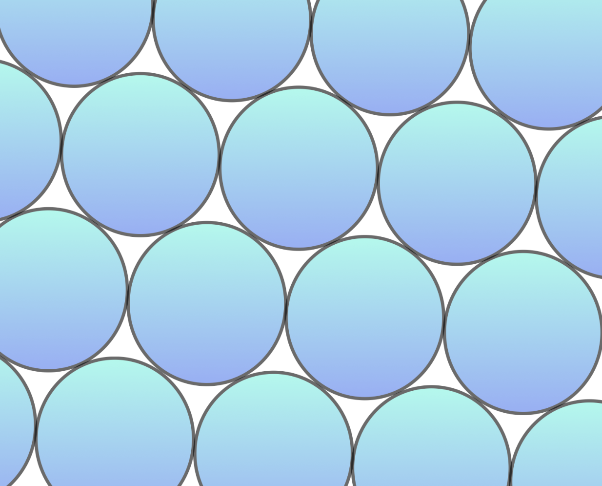
14.1 Intuition

The sphere packing problem traces its roots back to Kepler, and it asks for a packing of solid spheres in Euclidean space that achieves the maximum possible density. In all of the known cases, such optimal configurations - for the centers of the spheres - form a lattice. It’s natural, therefore, that Fourier analysis comes into the picture. We prove here a result of Cohn and Elkies, from , which is a beautiful application of Poisson summation, and gives certain upper bounds for the maximum densities of sphere packings in .
At this point it may be wise to define carefully all of the terms - what is a packing? what is density? Who was Kepler?
14.2 Lattice sphere packings
A lattice sphere packing in is a packing of balls, all having the same radius, with the property that the centers of the balls are located precisely at the points of some fixed lattice , as in Figure 14.3.
A densest lattice sphere packing is a lattice sphere packing with the additional property that no spheres with a larger radius will form a packing.
Example 14.1.
In Figure 14.3, we’ve used the same lattice for two distinct sphere packings: on the left, we have a sphere packing that is not optimal, and on the right we have a sphere packing that is optimal. But there are other lattices in that give us a sphere packing with a higher density. A natural question comes to mind: can we find a lattice that achieves the largest possible packing density?

Suppose we fix a lattice and we have an optimal (densest) lattice packing with respect to . To quantify the packing density for a lattice sphere packing, we may think of “how many balls of radius do we have per unit volume of the lattice ”?
We recall that is the ball of radius in , and that is the ball of radius . If we have a densest lattice sphere packing for a fixed lattice , then we define its lattice packing density, relative to , by the expression:
| (14.1) |
It’s easy to see that to achieve the densest possible lattice sphere packing with this particular , we should use , which is half-way from the origin to a nearest lattice point of . In other words, we may rewrite the expression (14.1) for the densest sphere packing of a fixed lattice as follows:
| (14.2) |
where we used .

Example 14.2.
Consider the integer lattice . It is clear that we can place non-overlapping spheres of radius at each integer point, as in Figure 14.4 on the left. It is also clear that any larger radius for our spheres will incur overlapping spheres. So this particular packing gives us a sphere packing density of
Example 14.3.
Now consider the hexagonal lattice as in Figure 14.4 on the right. It’s clear that we can still place non-overlapping spheres of radius at each of these lattice points. This particular arrangement of spheres gives us a packing density of
As it turns out, this is the densest lattice sphere packing, and Lagrange [143] was the first to prove it, in 1773.
More generally, suppose we are given a convex, compact, centrally-symmetric set . We may similarly define a densest packing density for , relative to any fixed lattice :
| (14.3) |
where we used definition (13.1) for the first successive minimima of relative to , namely .
But which lattice achieves the densest lattice sphere packing? This is clearly an extremely difficult problem in general, because it is a discrete optimization problem over an infinite-dimensional space of lattices. Nevertheless, we may define the densest lattice packing of , as we vary over all full-rank lattices :
| (14.4) |
where the supremum is taken over all full-rank lattices in .
Question 31 (The lattice sphere-packing problem).
For each dimension , find the value of , and find a lattice that achieves it.
Example 14.4.
In , we consider the ‘‘face-centered-cubic’’ lattice, defined by:
This lattice sphere packing gives us a packing density of
| (14.5) |
As it turns out, this is the densest lattice sphere packing, a statement that was first proved in 1831, by Gauss. In the notation of Question 32, Gauss proved that .
Example 14.5.
Putting some of the definitions above together, we arrive at the following elementary but useful equivalence.
Lemma 14.1.
Suppose we are given a convex, compact, centrally-symmetric set , with . The following are equivalent:
- 1.
There exists a lattice with , such that contains no nonzero points of .
- 2.
There exists a lattice such that .
14.3 More general sphere packings
In order to allow more general packings of spheres, we will relax the restriction of using just one lattice, as follows. A densest periodic sphere packing is a packing of spheres of radius , with a lattice , but also with a finite collection of its translates, say , such that the differences , and such that no larger radius will form a packing. Figure 14.5 gives such an example, by using lattices, rather than just one.

Given a period sphere packing with a lattice and a set of translates , we define its periodic sphere packing density by
| (14.6) |
corresponding to placing a sphere of radius at each point of , and also at each point of its translates . It’s not hard to prove that the latter definition 14.6 matches our intuition that any fixed fundamental parallelepiped of intersects this configuration of spheres in a set whose measure is exactly (Exercise 14.1).
The densest periodic sphere packing is defined by varying over all lattices, as follows.
| (14.7) |
where the supremum is taken over all full-rank lattices in .
Question 32 (The general sphere-packing problem).
For each dimension , find the value of , and find a lattice that achieves it.
Many other questions naturally arise.
Question 33.
Fixing the dimension , is ?
In other words, may we always use just one lattice to achieve a densest sphere packing? Or are there dimensions for which we need to use some translates of a lattice as well?
Question 34.
If the answer to Question 33 is affirmative, then is such an optimal lattice unique in each dimension?
It turns out that periodic sphere packings come arbitrarily close to arbitrary sphere packings, as shown in Appendix A of [56] (see also Greg Kuperberg’s paper [139]). So there is no loss of generality in merely considering periodic sphere packings for the general problem of sphere packings, as done by Cohn and Elkies [56].
With these news ideas in mind, we can revisit our densest lattice sphere packings in dimensions and , from Examples 14.3 and 14.4. In 1910, Axel Thue [235] was the first to prove that in we do indeed have
finally settling completely the question of the general sphere packing problem for (for any configuration of spheres of the same radius), a question that eluded even Gauss. In 1950, Laszlo F. Toth [238] extended the work of Thue, by allowing incongruent circles of different radii, among other extensions.
For , the famous astronomer Johannes Kepler conjectured in that the densest possible sphere packing was given by a lattice, namely the face-centered cubic lattice of Example 14.4. In 2005, Thomas C. Hales published a proof [103] that indeed
confirming that indeed Kepler was correct, and that . Hales’ proof, part of which was done with Sam Ferguson, was a huge breakthrough, even though it was a computer-aided proof.
In , is it true that the densest periodic sphere packing given by the lattice? It seems reasonable to conjecture that it is, but this is still open as well. The only dimensions for which we know the answers to Question 33 and Question 34 are , and in these known cases the answer is affirmative. Nevertheless, it seems reasonable to think that in higher dimensions the answer will become negative - there is more ’freedom to move around’. That is, it is widely believed that in higher dimensions, we might discover that often . Even in dimension , the densest known sphere packing is not a lattice packing. The sphere packing problem continues to intrigue, and it is a very important problem in Geometry, Number theory, Coding theory, and information theory.
14.4 Upper bounds for sphere packings, via Poisson summation
Here we give an exposition of the ground-breaking result of Henry Cohn and Noam Elkies on the sphere packing problem [56]. This result sets up the machinery for finding certain magical functions , as defined in Theorem 14.1 below, that allow us to give precise upper bounds on . The main tool is Poisson summation again, for arbitrary lattices. We recall that we defined a function to be nice if satisfies the Poisson summation formula
pointwise for all .
Theorem 14.1 (Cohn-Elkies).
Let be a nice function, not identically zero, which enjoys the following three conditions:
- 1.
, for all .
- 2.
, for all .
- 3.
, and .
Then the periodic sphere packing density has the upper bound:
Proof.
Suppose we have a periodic packing with spheres of radius , a lattice , and translation vectors
, so that by definition the packing density is
.
By Poisson summation,
we have
| (14.8) |
converging absolutely for all . Now we form the following finite sum and rearrange the right-hand-side of Poisson summation:
| (14.9) | ||||
| (14.10) |
Every summand on the right-hand-side of (14.10) is nonnegative, because by the second assumption of the Theorem, we have , so that the whole series can be bounded from below by its constant term, which for gives us the bound .
On the other hand, let’s ask what the positive contributions are, from the left-hand-side of (14.9). Considering the vectors on the left-hand-side of (14.9), suppose we have . Then the first hypothesis of the Theorem guarantees that . So we may restrict attention to those vectors that satisfy . Here the vector is contained in the sphere of radius , centered at the origin, but this means (by the packing assumption) that it must be the zero vector: . By assumption, the difference between any two translations is never a nonzero element of , so we have , and now . We conclude that the only positive contribution from the left-hand-side of (14.9) is the term, and so the left-hand-side of (14.9) has an upper bound of .
Altogether, Poisson summation gave us the bounds:
Simplifying, we have
Since the upper bound does not depend on the lattice , we get the desired result. ∎
Example 14.6 (The trivial bound).
Let be a full-rank lattice in , whose shortest nonzero vector has length . We define the function
where is the ball of radius , centered at the origin. We claim that satisfies all of the conditions of Theorem 14.1. Indeed, by the convolution Theorem,
for all , verifying condition 2. Condition 1 is also easy to verify, because the support of is equal to the Minkowski sum (by Exercise 5.10) , a sphere of radius . It follows that is identically zero outside a sphere of radius . For condition 3, by the definition of convolution we have . Finally, .
By the Cohn-Elkies Theorem 14.1, we know that the packing density of such a lattice is therefore bounded above by
the trivial bound. So we don’t get anything interesting, but all this tells us is that our particular choice of function above was a poor choice, as far as density bounds are concerned. We need to be more clever in picking our magical .
Although it is far from trivial to find magical functions that satisfy the hypothesis of the Cohn-Elkies Theorem, and simultaneously give a strong upper bound, there has been huge success recently in finding exactly such functions - in dimensions and . These recent magical functions gave the densest sphere packings in these dimensions, knocking off the whole sphere packing problem in dimensions and .
Another observation that is useful is that if we have a magical function that enjoys all three hypotheses of the Cohn-Elkies Theorem 14.1, then also satisfies the same hypotheses, for any (Exercise 14.5). We may therefore take certain radial functions as candidates for magical functions.
As of this writing, the provably densest packings are known only in dimensions , and . Each dimension seems to require slightly different methods, and sometimes wildly different methods, such as . Somewhat surprisingly, the sphere packing problem is still open in all other dimensions.
14.5 Lower bounds for sphere packings
Here we discuss lower bounds for the optimal sphere packing problem. As always, things began with Minkowski.
Theorem 14.2 (The Minkowski-Hlawka theorem, 1943).
Let be a -dimensional centrally symmetric convex body. Then we have:
| (14.11) |
where is the Riemann zeta function.
Minkowski proved (14.11) in the special case that , the unit ball in , and he conjectured that the same lower holds for all centrally symmetric convex bodies. This particular conjecture of Minkowski was finally proved by Hlawka [118]. We recall that a unimodular lattice simply enjoys . To prove Theorem 14.2, Hlawka first proved the following interesting fact (in a straightforward manner) concerning the existence of a certain unimodular lattice [118].
Lemma 14.2 (Hlawka, 1943).
Let be a bounded, real-valued, compactly supported function. For each , there exists a unimodular lattice such that
| (14.12) |
In 1945, Carl Ludwig Siegel extended Hlawka’s Lemma 14.2 with the following fundamental fact [222]. To state this result, we will need to assume a bit more background of the reader, just for the remainder of this section. By way of introductions, the group (which is a very important Lie group in Number theory and physics), may be thought of as the space of all unimodular lattices in .
Theorem 14.3 (C. L. Siegel, 1945).
Let be a bounded, compactly supported function. Then:
| (14.13) |
where is the unique normalized Haar measure on , and the matrix varies over .
So Hlawka’s Lemma 14.2 follows immediately from Siegel’s Theorem 14.3, even with . As another example, let’s consider the special case of , where is any bounded, measurable subset of . Here (14.13) gives us the intuitively compelling conclusion that as varies over all unimodular lattices in , the number of nonzero lattice points in is “on average” equal to the volume of (where this “average” is really the integral over the space of all unimodular lattices). The reader may also consult Zong [256], for a proof of Theorem 14.3.
In 1992, Keith Ball [9] improved upon the Minkowski-Hlawka theorem, and gave the following lower bounds, which included a new linear term.
Theorem 14.4 (Ball, 1992).
where is the -dimensional unit ball.
For large dimensions, is very close to , so some authors omit the factor of .
In 2013, Akshay Venkatesh [244] has given an improvement over the known lower bounds, by using a variation of Siegel’s Theorem 14.3 above.
Theorem 14.5 (Venkatesh, 2013).
There exist infinitely many dimensions for which
In addition, for all sufficiently large dimensions, we have .
Notes
- 1.
Each dimension appears to have a separate theory for sphere packings. This intuition is sometimes tricky to conceptualize, but there are facts that help us do so. For example, it is a fact that the Gram matrix (see 6.29) of a lattice consists entirely of integers, with even diagonal elements is divisible by . For this reason, it turns out that the theta series of a lattice possesses certain functional equations (making it a modular form) if and only if , which in turn allows us to build some very nice related ‘magical’ functions that are sought-after in Theorem 14.1, at least for and so far.
In dimension , it is an open problem to find such magical functions, even though there is an independent proof that the hexagonal lattice is the optimal sphere packing lattice.
- 2.
Johannes Kepler (1571 --1630) was a German astronomer and mathematician. Kepler’s laws of planetary motion motivated Sir Isaac Newton to develop further the theory of gravitational attraction and planetary motion. Kepler conjectured that the densest packing of sphere is given by the ‘‘face-centered cubic’’ packing. It was Gauss (1831) who first proved that, if we assume the packing to be a lattice packing, then Kepler’s conjecture is true. In Thomas Hales (using an approach initiated by L. Fejes Tóth (1953)), gave an unconditional proof of the Kepler conjecture.
- 3.
It is also possible, of course, to pack other convex bodies. One such variation is to pack regular tetrahedra in . The interesting article by Jeffrey Lagarias and Chuanming Zong [142] gives a nice account of this story. For a classical introduction to sphere packings, the reader may also consult the book by Chuanming Zong [256]. There is also a nice survey paper on many other aspects of packings, coverings, and tilings by Zong [257].
- 4.
We mention some of the recent spectacular applications of the Cohn-Elkies Theorem. In 2016, Maryna Viazovska was able to find these magical functions for , thereby proving that the lattice gives the densest sphere packing in dimension . Shortly afterwards, professor Viazovska, joined with the team effort of Henry Cohn, Abhinav Kumar, Stephen D. Miller, and Danylo Radchenko, managed to also find magical functions in [55]. Here is a synopsis of some of their results.
Theorem 14.6 ([55]).
The lattice is the densest periodic packing in . The Leech lattice is the densest periodic packing in . In addition, these lattices are unique, in the sense that there do not exist any other periodic packings that achieve the same density.
Exercises
“It is better to do the right problem the wrong way, than the wrong problem the right way.”
-- Richard Hamming
14.1.
Given a periodic lattice packing, by translates of a lattice , show that any fixed fundamental parallelepiped of intersects the union of all the spheres in a set of measure , where . Thus, we may compute the density of a periodic sphere packing by just considering the portions of the spheres that lie in one fundamental parallelepiped.
14.2.
Here we show that the integer lattice is a very poor choice for sphere packing.
- 1.
Compute the packing density of the integer lattice .
- 2.
Compute the packing density of the lattices and .
- 3.
Compute the packing density of the lattices , for .
14.3.
If is a radial function, then prove that its Fourier transform is also a radial function.
14.4.
Suppose we pack equilateral triangles in the plane, by using only translations of a fixed equilateral triangle . To make the problem easier, we’ll restrict attention to lattice packings here. What is the maximum lattice packing density of ? Do you think it may be the worst possible density among lattice packings of any convex body in ?
14.5.
Show that if we have a magical function that enjoys all hypotheses of Theorem 14.1, then also satisfies the same hypotheses, for any orthogonal transformation .
14.6.
We define a rigid motion of a compact set to be any orthogonal transformation of , composed with any translation of .
- 1.
When , find a continuous function (other than the zero function) such that:
for all constants .
- 2.
More generally, in any dimension , find a (nontrivial) continuous function that allows the following integrals (taken over any ball of radius ) to vanish:
for all constants .
Notes. For part 2, it’s advisable to think about the Fourier transform of the ball. It is conjectured that for any bounded set with nonempty interior, the balls in this example are the only examples of objects that allow such nonzero continuous functions to exist. This is known as the Pompeiu problem - see also Question 15.
14.7.
14.8.
Show that the Hermite constant is very simply related to the densest lattice sphere packing density by:
| (14.14) |
14.9.
14.10.
Prove Lemma 14.1.
Chapter 15 Shannon sampling, in one and several dimensions
“It is easy to argue that real signals must be band-limited.
It is also easy to argue that they cannot be so.”-- David Slepian
(Under construction)
15.1 Introduction
Sampling theory consists in the reconstruction of a continuous function with only a discrete or finite amount of data and has many applications in signal processing and other engineering applications. At a first glance this task sounds impossible, however it can be done well in practice. One of the reasons for this success comes from the Fourier analysis, which deals with the representation of a function in terms of its “frequencies”, and functions without high frequencies (bandlimited) represents very well the real-world signals.
In one dimension, the classical example is a sound signal, and since typical humans can only hear sounds with frequencies smaller than kHz, the bandlimited assumption is appropriate. Examples in higher dimensions include images or MRI exams where higher frequencies are associated with random noises and measurement errors, more connected to the physical apparatus than the object being measured [80]. In this sense it is even desirable to remove the high frequency information.
More recently, the interest in bandlimited functions increased in the machine learning community, because it was observed that neural networks learns low frequencies faster and this might explain why they often generalize quickly from the training sets.
On the other hand, by a basic uncertainty principle of Theorem 4.23, we know that a function with compact support can never be bandlimited, so representing an arbitrary function using this class of functions is in general not exact. It is therefore desirable to also give some theoretical results concerning the error of such approximations.
Here we introduce the classical sampling theorem by Shannon and Whittaker for one dimensional sampling, and then we study some of its generalizations to higher dimensions, where much less is known. An excellent introduction to Sampling Theory, from an expository as well as a rigorous perspective, is the book of J. R. Higgins [116].
15.2 The Shannon-Whittaker sampling Theorem
Claude Shannon [218] showed how to reconstruct a complete signal by sampling it only discretely, in a classical paper that gave rise to the field of information theory. To accomplish this, Shannon used an interesting assumption, namely that the Fourier transform of vanishes outside of some interval.
One of the main characters of this story is our old friend, the function:
| (15.1) |
which plays a central role in the sampling theory for functions in , because it turns out to be a building block for a basis of the Paley-Wiener space , as the Shannon-Whittaker sampling theorem shows.
Reviewing some of the Fourier facts that we learned in Chapter 4, we recall that if , then is uniformly continuous and as . So not every function can be the Fourier transform of some other function in .
In practice, we are often interested in functions that are not absolutely integrable, and yet possess a (conditionally convergent) Fourier transform, such as the important function. To resolve this issue, the theory progresses by first defining the transform in the space , and then extending the definition of to all of , by taking the limit . This unique extension of the Fourier transform, from the space to the space, is sometimes called the Plancherel-Fourier transform. From now on, we’ll follow the usual Fourier convention and simply call both transforms “the Fourier transform”.
For a given number , a function is called c-bandlimited if
| (15.2) |
We will sometimes just say ‘bandlimited’ if the is not contextually important. A bandlimited function has a Fourier transform that decays at the ‘best possible rate’, in the sense that its Fourier transform is identically zero outside the interval . It’s easy to notice that any -bandlimited function must be equal (almost everywhere) to an infinitely smooth function, because by Fourier inversion, we have:
| (15.3) |
This identity implies that we can differentiate the last expression with respect to as many times as we like under the integral sign, because the integrand is a smooth function of , and we are integrating over a compact domain. Therefore is infinitely smooth. For simplicity, when considering a bandlimited function , we will always assume that is also continuous, which is consistent with the equality in (15.3).
Given any , we define the space of all -bandlimited functions in by
called the Paley-Wiener space [116].

Theorem 15.1 (Shannon-Whittaker).
Suppose that . Then we have
| (15.4) |
and the series converges absolutely and uniformly over .
In other words, if we sample a -bandlimited function at only the discrete set of points , we may reconstruct the whole function for all ! In the next two sections, we give two different proofs of Theorem 15.1.
The quantity is called the sample spacing and its reciprocal is the sampling rate. So what the theorem says is that to reconstruct a function with bandlimit , one has to sample at a rate . Offhand, it seems rather incredible that some (non-periodic) functions may be completely recovered by knowing only their values at a discrete set of points. This phenomenon shows, in a sense, how the Paley-Wiener space is a very special subspace of .
15.3 The approach of G. H. Hardy
G. H. Hardy’s proof [104] of Theorem 15.1 is particularly interesting because it also answers the following informal question:
Question 35.
[Rhetorical] How large is the space of bandlimited functions?
Hardy’s approach also clarifies some of the underlying structure of bandlimited functions. It relies on the following isometry.
Lemma 15.1.
The Fourier transform gives a bijection between the following two Hilbert spaces:
Moreover, this bijection is an isometry.
Proof.
First, given any , we need to show that . By definition is -bandlimited, hence its Fourier transform can be naturally viewed as a function with domain . We need to show that has a finite norm. The following computation uses Parseval’s identity, namely that :
| (15.5) |
proving that .
Conversely, given any , we need to show that . We may extend to be equal to outside the interval , so that now . By construction of , we also have , so that now Lemma 4.3 guarantees that is uniformly continuous on . Because the Fourier transform is an isometry of , and , we also have . So now we have .
Finally, the Fourier transform is invertible, and since we have by Parseval again, we have an isometry between the two Hilbert spaces and . ∎
Hardy’s insight is to consider an orthonormal basis for and then pull it back to an orthonormal basis for . We recall the classical fact (Theorem 4.5) that the set of exponentials
form a complete orthonormal basis for the Hilbert space . Moreover, any has a unique representation in this basis (which we called its Fourier series), that converges in the -norm on :
| (15.6) |
with coefficients equal to
| (15.7) |
Using the Fourier series (15.6), we may expand , obtaining
Although we’ve only scratched the surface, we’ve already scratched it enough in order to prove Theorem 15.1.
Proof of Theorem 15.1.
For any , we know by Lemma 15.1 that , so that has a Fourier series that converges in the -norm on :
with coefficients equal to by the Fourier inversion formula (15.3). It follows that
| (15.8) |
From the orthonormality of the exponentials and Parseval’s identity (Lemma 15.1) we have
| (15.9) |
We recall that the equality in the norm in (15.8) means that
Using the Fourier inversion and the isometry stated in Lemma 15.1,
and therefore
| (15.10) |
To pass from the convergence in the norm to pointwise convergence, we need to show that the latter series converges uniformly, so that we can conclude that it represents a continuous function and hence by Lemma B.3 it is equal to everywhere.
To prove the uniform convergence, we make use of the Cauchy-Schwartz inequality for infinite series, namely
| (15.11) |
The rest of the proof consists in showing that the right-hand side of (15.11) goes to zero as , uniformly for . The same proof will also work for the series defined from to . Together these results show that the expression in (15.10) converges absolutely and uniformly over , giving the result stated in the theorem. From (15.9), we see that
| (15.12) |
Clearly
and since the latter series are periodic function of , with period , we may assume that . For and , we note that . For , we use the estimate
so that
Similarly, for ,
We conclude that for all , , and therefore the series in (15.11) converges uniformly to as . ∎
It follows from this approach of G.H. Hardy, that despite being a subspace of , the Paley-Wiener space has a concrete, countable basis, which we record as follows.
Corollary 15.1.
The set of translated functions
| (15.13) |
is a complete orthonormal basis for the Hilbert space of -bandlimited functions.
It is also worthwhile recording here the orthonormality of the functions explicitly. For each , we have:
| (15.14) |
15.4 An alternative proof, using Poisson summation
Here we give Shannon’s proof of the classical Shannon-Whittaker sampling theorem (Theorem 15.1), with some added details. This proof uses the Poisson summation formula. As we’ve seen several times before, Poisson summation often simplifies proofs in surprising ways.
To state the formula more precisely, we use and to denote convergence in the -norm, so that equality between functions holds almost everywhere but cannot be assumed at a specific point, unless we have an additional assumption like continuity.
Assuming only that , the Poisson summation formula (See [232]) states that the periodized function defined by the series converges in the norm of to a function whose Fourier expansion is
| (15.15) |
Proof of Theorem 15.1.
We begin with the Fourier series (15.15), which converges in the norm.
Step . Our first goal will be to exchange the roles of and . To justify this, we begin by noting that our assumption that implies by Lemma 15.1, and by Lemma 4.7. So we have , allowing us to apply the same Poisson summation formula as above, together with Fourier inversion:
| (15.16) |
Step . Since we are assuming that and thus is supported on , we may use the indicator function , defined as if and otherwise, and write the trivial identity
| (15.17) |
for all real . The reason is that the series on the right-hand-side contains only one term, namely the term .
Step . Using the Poisson summation formula (15.16) above, together with (15.17), we see that
| (15.18) |
We recall that the inverse Fourier transform of the interval is
so that after composing the function with a translation, we know that the Fourier transform of is . Multiplying both sides of (15.18) by and integrating term-by-term over , we get:
applying Fourier inversion again on the left-hand side.
Finally, we recall that we are assuming is continuous, since . So to pass from the convergence in the norm to the pointwise convergence we may apply the same procedure from the first proof to conclude that the series on the right converges uniformly in and hence also represents a continuous function. ∎
There are many different possible extensions of the Shannon-Whittaker sampling theorem to higher dimensions, and below we glimpse some of them below.
15.5 Special properties of bandlimited and sinc functions
Here we focus on some special properties of bandlimited functions. We’ve already seen in Section 15.3 that the space is isometric to , so many of its special properties comes from , and they are then pulled back via inverse Fourier transform.
The special case of Theorem 15.1 is worth pointing out:
| (15.19) |
a classical version of the Shannon-Whittaker formula. The choice of means that we begin with the interval in the frequency space; this interval is a Voronoi cell of the integer lattice .
Example 15.1.
What happens if we apply the Shannon-Whittaker formula (15.19) to the function itself? Let’s try it!
With , and any fixed , we have:
| (15.20) |
As a special case, if we let , we get:
| (15.21) |
In Corollary 15.1 we showed that the functions with form an orthonormal basis for the space of bandlimited functions. This has some nice consequences.
Theorem 15.2.
If and are -bandlimited, then
[Intuitive proof] If we work formally, then we can use the orthonormality of the sinc functions (15.14), together with (15.19) to quickly see that:
and we’re done. Although this intuitive proof may seem ‘fast and loose’, these steps can be made rigorous if we would prove just a bit more about Hilbert spaces, because the Paley-Wiener space is a Hilbert space, and the translated functions are a basis for this Hilbert space.
One important case of the previous theorem is when , which combined again with the Shannon-Whittaker formula (15.19) results in the next theorem.
Theorem 15.3.
The space is a space with a reproducing kernel , which means by definition that any can be written as
Proof.
We also have the following somewhat surprising properties of bandlimited functions on . First we recall that we called a nice function if , and satisfies the Poisson summation formula:
| (15.22) |
valid pointwise for each .
Theorem 15.4.
Let be a nice function, such that is -bandlimited. Then we have:
- 1.
We have, for each ,
(15.23) We note that the identity (15.23) can be interpreted to mean that the Riemann approximation to the integral is always exact for such an , provided that the step size is .
- 2.
For all with and , we have
(15.24)
Proof.
To prove 1, we use Poisson summation (15.22), with :
| (15.25) |
which is the desired identity. In the last equality we used the assumption that the indices of summation satisfy , for , so that because is -bandlimited by assumption. We also used the fact that .
To prove 2, we apply the following small variation of Poisson summation:
| (15.26) |
which follows quickly from the Poisson summation formula given above in (15.22) (Exercise 15.3). But by the assumption that is -bandlimited, we also have
| (15.27) |
provided that
| (15.28) |
For , we see that a necessary condition for (15.28) is . Geometrically, (15.28) tells us that the arithmetic progression does not intersect the interval . It is easily checked that the additional constraint gives us a sufficient condition for (15.28) to hold. ∎
As is easily observed, sums and products of bandlimited functions are again bandlimited. In particular, more precise statements such as the following are possible.
Lemma 15.2.
Suppose that is -bandlimited, and is -bandlimited.
Then is -bandlimited.
Proof.
By assumption, outside of , and outside of . We need to show that vanishes outside the interval . We also have, by assumption, that , and since (Lemma 4.7), it follows that . Therefore the convolution Lemma 4.12 2 applies:
We know that the support of the convolution is contained in the closure of the Minkowski sum of the individual supports of and (by Exercise 5.10), which is equal to . ∎
Example 15.2.
Here are some fun consequences of Theorem 15.4. Let’s fix any . By Theorem 15.4, part 2 , we can pick , and , all of which satisfy the hypothesis, so that is -bandlimited by definition. We then have
| (15.29) |
Seperating the lattice sum into even and odd, we have
| (15.30) |
Generalizing the latter identity, we fix any positive integer , and we let , and , so that is -bandlimited by definition. By Theorem 15.4, part 2:
| (15.31) |
so that we get the identity
| (15.32) |
Example 15.4.
Consider , which has the bandlimit . By Theorem 15.4, the strange relation
| (15.33) |
holds for , because in this range we have . It’s also true for , with some care:
It turns out that this identity fails, however, for . Indeed, by Poisson summation (15.22), for a nice function we have:
Taking , we see that that the last sum is zero when and positive when , since has support and is positive inside this interval.
In a similar manner to eq. (15.33), we have:
| (15.34) |
holds for , since for these we have . It can be also checked that the equality above fails for . These facts are easy corollaries of Theorem 15.4, but may seem surprising when taken out of this context. The identities (15.33) and (15.34) appeared in [7].
15.6 Shannon sampling in higher dimensions
The first research into higher-dimensional Shannon-type sampling theorems, as far as we know, was the work of Petersen and Middleton [180]. We’ll also follow a bit of Chapter from Higgins [116].
For a convex body , we say that a function is -bandlimited if vanishes outside of . We note that this does not preclude the possibility that may only be nonzero on some proper subset of . Assuming that is real-valued, we know that the image of is symmetric about the origin (Lemma 5.2); so the assumption that is symmetric is natural.
By analogy with the -dimensional Paley-Wiener space , we define the Paley-Wiener space of -bandlimited functions in :
| (15.35) |
A new twist in higher dimensions is the strong distinction between packing and tiling, so the following question motivates some of these research directions.
Question 36.
Given a convex -dimensional body , suppose we want to have a sampling theorem for functions that are -bandlimited. Does have to tile by translations, or is it sufficient to consider a packing of by some lattice ?
Interestingly, we don’t observe this distinction in dimension , because optimal packing and tiling are equivalent. But they are quite different in dimensions . Luckily, our elementary -dimensional Lemma 15.1 does extend directly to our new -dimensional setting.
Lemma 15.3.
Let be a bounded convex body in . The Fourier transform is an isometry between the two Hilbert spaces:
Proof.
Given , by definition , so using Parseval’s identity we have:
| (15.36) |
which shows that . Using the fact that the Fourier transform is an isometry of , and is invertible, we are done. ∎
Now this chapter comes full circle with the goals of the previous chapters: to better understand the Fourier transform of a convex body. The following result helps.
Theorem 15.5 (Higher-dimensional sampling formula).
Suppose we have a lattice packing for a symmetric convex body , with a lattice . If , then then we can reconstruct the function completely by sampling it only at the lattice points of :
and the series converges absolutely and uniformly over .
Proof of Theorem 15.5.
The assumption that , together with being compact, implies that . Now we may use the Poisson summation formula (15.22), but with replaced by , and with replaced by :
| (15.37) |
where we also have used that . Because is supported on , we have by definition , so that we may write
| (15.38) |
for all that do not lie on the boundary of .
Because of our packing assumption, all of the translated supports of are disjoint, as varies over the lattice . In other words, these supports are
a disjoint collection of translates of . This means that the latter identity (15.38) holds because the series on the right-hand-side contains only one term, namely the term . Next, we combine (15.37) with (15.38) to get
| (15.39) |
Now we’d like to take the inverse Fourier transform of both sides of (15.39). We’ll use the following elementary identity, for a fixed :
We finally arrive at
To finish the proof, we just to pass from the -convergence of the latter identity, to its pointwise and uniform convergence. The series converges uniformly on by a standard argument, as in [116] for example. ∎
Let’s conduct a sanity check and verify that Theorem 15.5 indeed generalizes Theorem 15.1, the classical -dimensional Shannon-Whittaker sampling theorem. In the one dimensional case, the lattice is just the sampling domain and hence , while is simply an interval. Therefore:
The formula from Theorem 15.5 reduces to the formula from Theorem 15.1:
which is the Shannon-Whittaker sampling formula.
Intuitively, if we pick a larger set , then the vectors from will have to be more widely spaced in order to satisfy the packing condition for . Therefore in Theorem 15.5, we will need to sample from a denser lattice , due to the reciprocal relation .
On the other hand, for a given sampling lattice , in this multidimensional case we can consider infinitely many different bodies that form a packing of with the lattice . One of the most natural choices for such a convex set is the Voronoi cell of .
In closing, we note that it is impossible for both and to be simultaneously bandlimited, by the basic uncertainty principle, Theorem 4.23. However, in practice, if we are given a function that is not bandlimited, we can form a sequence of bandlimited functions that approach as , as follows. To make compactly supported, we’ll multiply by , the indicator function of the cube. Pulling things back to the space domain, we have:
| (15.40) | ||||
| (15.41) |
So if we define , then , a compactly supported function that is bandlimited to the cube .
The careful reader might notice that in (15.41), we are really applying the Fourier inversion formula on (as opposed to the Fourier inversion formula on )). We do this because although , we do have .
Notes
- 1.
John Higgins’ book [116], Chapter , has an excellent account of the Paley-Wiener space, and its connections to the Paley-Wiener theorem, which also answers the question: “how may we analytically continue bandlimited functions of a real variable, to ?” Moreover, Higgin’s book has more mathematical rigor than many other books that treat sampling.
- 2.
- 3.
Interesting relations between rates of convergence of bandlimited functions, Nikol’skij type functions spaces, and Plancherel-Polya type inequalities is given in [212].
Exercises
“The only true wisdom is in knowing you know nothing.”
-- Socrates
15.1.
By using an example, show that a bandlimited function may not be in .
15.2.
Let , and fix any . Prove that is completely determined by the samples
15.3.
Here we give another small variation on Poisson summation, namely that for any , we have
| (15.42) |
where is a nice function (in the sense of (15.22)).
15.4.
Consider the function , when .
- 1.
Show that is -bandlimited.
- 2.
Show that for each , we have:
using any results from this book.
- 3.
Show that .
Appendix A The dominated convergence theorem, and other goodies
A frequent question that comes up in proofs is “when may we take the limit inside the integral”? A general tool that allows us to do so is the Dominated convergence theorem. Here we remind the reader of some of the basic results from real analysis, but we skip the proofs and give references for them. For our purposes, we only need these results in Euclidean spaces, although all of these theorems have extensions to arbitrary measure spaces. All functions here are assumed to be measurable.
Theorem A.1 (Fatou’s lemma).
Fixing any subset , let be a sequence of nonnegative functions. Then we have:
| (A.1) |
The inherent flexibility in Fatou’s lemma allows it to be useful in many different contexts, because the lim inf always exists, and are even allowed to be equal to infinity. In fact, Fatou’s lemma is the main tool in proving Lebesgue’s dominated convergence theorem, below.
Another essential fact for us is Fubini’s theorem, which allows us to interchange integrals with integrals, and series with integrals, for product spaces. If we write , and we denote a point by , then we may also write .
Theorem A.2 (Fubini).
Let . Then:
| (A.2) |
and
| (A.3) |
There is also a version of Fubini’s theorem that uses the counting measure in one of the factors of , giving us:
| (A.4) |
A.1 The Dominated Convergence Theorem
Theorem A.3 (Dominated convergence theorem).
Suppose that we have a sequence of functions , for , and suppose there exists a limit function , valid for all .
If there exists a function such that for all , we have:
then:
- 1.
.
- 2.
.
- 3.
And finally, we may interchange limits and integrals:
Theorem A.3 is sometimes called the Lebesgue dominated convergence theorem, honoring the work of Lebesgue. There is a useful application of Lebesgue’s dominated convergence theorem, which allows us to interchange summations with integrals as follows.
Theorem A.4.
Suppose that we have a sequence of functions , such that
Then the series converges for all , and we have:
A.2 Big-O and Little-o
Very often we’d like to compare, in a quick-and-dirty way that avoids uncountably many details, how fast two functions grow. We review here two of the most common ways to do this.
Suppose we are given two functions . We say that (pronounced “Big o”), as , if there exists a positive constant such that
| (A.5) |
for all that are sufficiently close to . Here we allow to be any real vector, and we also allow the very common case . Equivalently, we may say
Example A.1.
We write , as . We could, of course, also write , though the former way of writing it is much more common. In this case, we can give a ‘better’ Big-O estimate by adding more terms of the Taylor series: , as .
Example A.2.
Given , and , we have
In other words, for all sufficiently large , , despite the fact that this statement is false for these particular functions, for some small positive values of .
Claim. Big-O enjoys transitivity:
Proof.
For all sufficiently close to , there exists positive constants such that and , implying that
∎
There is another very useful comparison technique, for any two given functions . We say that (pronounced “little o”), as , if for all positive constants , we have:
| (A.6) |
for all that are sufficiently close to . Again we allow to be any real vector, and we also allow the very common case . Equivalently, we may also write
which intuitively means that approaches faster than does.
Example A.3.
Given , and , where we restrict the domain of both functions to be . We claim .
Proof.
So approaches much faster than . ∎
Claim. Little-o also enjoys transitivity:
Proof.
The two given limits and together imply that
∎
Appendix B Various forms of convergence
B.1 Weierstrass M-test
How can we quickly conclude that certain series converge uniformly? The following criterion, discovered by Karl Weierstrass, comes to the rescue. For the proofs of these basic real analysis results, see for example the classic [202].
Theorem B.1.
[Weierstrass M-test] Suppose that is a sequence of complex-valued functions defined on a set , such that there exists a sequence of numbers satisfying the following conditions:
- 1.
.
- 2.
.
Then the series converges absolutely and uniformly on .
In practice, the Weierstrass -test gets used together with the following test, which allows us to partially answer the question:
Question 37.
When does a series converge to a continuous function of ?
Theorem B.2.
[Uniform limit] Suppose that is a sequence of continuous functions defined on a set , and that converges uniformly to , on . Then is continuous on .
B.2 Some things you wanted to know about convergence but were afraid to ask
It’s often useful to pass from convergence to pointwise convergence, under some additional hypothesis on . Throughout, we fix a real number . Given a measurable subset , and a sequence of functions , we say that in the -norm if
| (B.1) |
for which we will also use here the notation . Sometimes, if the constant is not specified, it is common to simply call (B.1) convergence in norm. The two most common subsets are , and . A natural question arises:
Question 38.
When can we pass from convergence in norm to pointwise convergence?
Given a series , we consider the sequence of partial sums . By definition, we say the series converges
- 1.
pointwise on if the sequence converges, for each .
- 2.
absolutely on if the series converges pointwise, for each .
- 3.
uniformly on if the sequence of partial sums converge uniformly on .
- 4.
in the -norm on if .
Lemma B.1.
Consider the partial sums for all in a given subset . Suppose we have the following two properties:
- 1.
There exists a function such that in the -norm, on .
- 2.
converges uniformly to the series on .
Then .
Lemma B.2.
Let , and suppose we already know that its Fourier series converges pointwise:
| (B.2) |
If the series (B.2) converges absolutely, then is a continuous function on , and .
Proof.
The idea is to use the uniform limit Theorem B.2, together with the fact that the summands are continuous functions of . So it remains to show that the convergence of the series is uniform.
where the penultimate equality holds because , and the last inequality holds by assumption. So by the -test, with , we have uniform convergence of the series. Finally, the claim is trivial, because . ∎
In the previous lemma, we could have also used the alternate notation of the circle , and rewrite everything in terms of it, which automatically incorporates periodicity. The following passage from convergence in the norm, to pointwise convergence, is often useful.
Lemma B.3.
Let be a continuous function, and write its Fourier series as
| (B.3) |
which by definition means that this series converges in the -norm.
If the series (B.3) converges absolutely, then it also converges pointwise and uniformly to , for all .
Proof.
Repeating the computation of the previous proof, we have:
Therefore by the -test again, converges uniformly to the series , for all . We also know, by Lemma B.2, that is continuous on . We still need to prove that the series converges to , but now we at least know that both hypotheses of Lemma B.1 are satisfied (with and ), and therefore .
To prove that for all , we observe that the summands are continuous functions of , and hence by the uniform limit theorem (Theorem B.2), the series is itself a continuous function of . Since is also continuous on , and almost everywhere, they must agree everywhere. ∎
B.3 Bump functions
Perhaps the easiest bump function to define is the function ([233], page 209):
where the constant is chosen so that . By definition, is compactly supported, on the unit ball. It turns out that is infinitely smooth. As usual, using we can build a family of integrable functions:
Thus, the family is an approximate identity.
More generally, a bump function is defined to be any infinitely smooth function that is compactly supported. By Lemma 4.9, we know that any such bump function lies in the Schwartz class . Clearly finite linear combinations of bump functions are again bump functions, making the space of bump functions a vector subspace of the space of Schwartz functions.
Often, a slightly more general sort of space than a Hilbert space is required. Suppose there exists a function called , defined from , that enjoys the following properties:
- 1.
(Strict positivity) , for all nonzero .
- 2.
(Symmetry) , for all .
- 3.
(Linearity) for any fixed , the function is linear, which means that
for all .
Then is called an inner product on , and is an inner product space (over ). Inner products also interact well with continuity, in the following precise sense ([78], p. 74):
Lemma B.4.
If in , and in , then .
We say that an inner product space is complete, relative to the distance function , if every Cauchy sequence in converges to a point of . Finally, we mention a basic fact about linear functions acting on complete inner product space.
Theorem B.3 (Riesz Representation Theorem).
Let be a complete inner product space (finite or infinite dimensional), and suppose that is a continuous linear functional on . Then there exists a unique such that
for all .
Appendix C Solutions and hints
“There are no problems - just pauses between ideas.”
– David Morrell, Brotherhood of the Rose
Chapter 2
Exercise 2.1 By Euler, we have , which holds if and only if , and . The latter two conditions hold simultaneously if and only if , with .
Exercise 2.2 Let , so that , using the fact that for all real numbers .
Exercise 2.4 By definition,
Exercise 2.5 Let , and note that we may write
Now, pick any such that . Consider
so that , and since by assumption , we have .
Exercise 2.6 We use the finite geometric series: . Now, if , then , so we may substitute this value of into the finite geometric series to get:
On the other hand, if , then .
Exercise 2.7
Therefore, using Exercise 2.6, we see that the latter sum equals exactly when , and vanishes otherwise.
Exercise 2.8 We begin with the factorization of the polynomial , with . Dividing both sides by , we obtain . Now substituting , we have .
Exercise 2.9 Suppose to the contrary, that a primitive ’th root of unity is of the form , where . Let , and , so that by assumption both and are integers. Thus , a ’th root of unity, with , a contradiction.
Exercise 2.14 We recall Euler’s identity:
which is valid for all . Using Euler’s identity first with , and then with , we have the two identities , and . Subtracting the second identity from the first, we have
Now it’s clear that , by Exercise 2.1.
Exercise 2.16 We will assume, to the contrary, that we only have one arithmetic progression with a common difference of , the largest of the common differences. We hope to obtain a contradiction. To each arithmetic progression , we associate the generating function
where , in order to make the series converge. The hypothesis that we have a tiling of the integers by these arithmetic progressions translates directly into an identity among these generating functions:
Next, we use the fact that we may rewrite each generating function in a ‘closed form’ of the following kind, because they are geometric series: . Thus, we have:
Now we make a ‘pole-analysis’ by observing that each rational function has poles at precisely all of the ’th roots of unity. The final idea is that the ‘deepest’ pole, namely , cannot cancel with any of the other poles. To make this idea precise, we isolate the only rational function that has this pole (by assumption):
Finally, we let , to get a finite number on the right-hand-side, and infinity on the left-hand-side of the latter identity, a contradiction.
Chapter 3
Exercise 3.1 If , we have . If , we can compute the integral:
Exercise 3.2 Beginning with the definition of the Fourier transform of the unit cube , we have:
valid for all , except for the finite union of hyperplanes defined by
.
Exercise 3.4 To see that the generating-function definition of the Bernoulli polynomials in fact gives polynomials, we first write the Taylor series of the following two analytic functions:
Multiplying these series together by brute-force gives us:
| (C.1) | ||||
| (C.2) | ||||
| (C.3) |
The coefficient of on the LHS is by definition , and by uniqueness of Taylor series, this must also be the coefficient on the RHS, which is seen here to be a polynomial in . In fact, we see more, namely that
which can be written more cleanly as .
Exercise 3.5 Commencing with the generating-function definition of the Bernoulli polynomials, equation 3.13, we replace with in order to observe the coefficients :
where the last equality follows from the definition of the same generating function, namely equation 3.13, but with the variable replaced by . Comparing the coefficient of on both sides, we have .
Exercise 3.6 To show that , we play with:
Therefore, again comparing the coefficients of on both sides, we arrive at the required identity.
Exercise 3.7 We need to show that . Well,
so that comparing the coefficient of on both sides, the proof is complete.
Exercise 3.22 We’ll prove part 2. To begin, we have:
So it suffices to show that , for all . In other words, the problem is reduced to the Calculus I problem of showing that , for . To prove this, we let , so that it suffices to prove that on . Computing its derivative, on , and since , we conclude that is an increasing function. This proves on .
Exercise 3.27 For part (a), suppose to the contrary that none of the vertices of have degree . Because each of its vertices must have degree at least , then all of vertices have degree . By the ‘handshanking lemma’ of elementary graph theory, we have:
a contradiction. To prove part (b), consider the unit cube in , and take vertices that belong to one facet, with one vertex from an oppostive facet. It’s clear that all of its vertices have degree .
Exercise 3.31 Considering the partial sum , we know by Abel summation that
for each , where . By assumption, , and the ’s are going to , so we see that the first part of the right-hand-side approaches zero, namely: , as .
Next, we have
where the last equality holds because by assumption the ’s are decreasing. But the last finite sum equals , and we have , a finite limit. Therefore converges absolutely, and so converges, as desired.
Exercise 3.33 We fix , and let , which lies on the unit circle, and by assumption . Then
| (C.4) |
because . We also have
so that we have the equality . Altogether, we see that
| (C.5) |
Exercise 3.34 We fix and need to prove that converges. Abel’s summation formula (3.76) gives us
so that
and the latter series in fact converges absolutely.
Chapter 4
Exercise 4.1 For all four inequalities, we will use an arbitrary vector . For the first inequality, .
The second inequality means that , which is clear by squaring both sides.
To prove the third and most interesting inequality here, we use the Cauchy-Schwarz inequality, with the two vectors and :
which also shows that we obtain equality if and only if is a scalar multiple of .
For the fourth inequality, we have:
Exercise 4.2 To prove part (a), we compute:
To prove part (b), we begin with the definition of the hyperbolic cotangent:
Recalling the definition of the Bernoulli numbers, namely we see that
so the only surviving terms in the latter series are the terms whose index is an even integer. This yields
Exercise 4.3 We know, by equation (4.47), that the Fourier transform of is equal to . So using Poisson summation, we have:
Exercise 4.20 We are given that , and we wish to prove that is always continuous on . By definition, we need to show that .
To prove part 1, we fix any sequence of functions with the property that in . We’ll prove that , for each . Well, we have:
| (C.6) | ||||
| (C.7) | ||||
| (C.8) |
using the triangle inequality for integrals in (C.6), and the Cauchy-Schwartz inequality in (C.7). Since in , we are done. For part 2, we must show that
as . First we’ll show that the latter integral converges for each fixed nonzero vector :
using , and the Cauchy-Schwartz inequality for . We therefore have convergence of the integral for each nonzero . Next, we’ll separate the integral into two pieces, one of which is a ‘neighborhood of infinity’:
By the convergence of the integral, we know that given any , there exists such that
It remains to handle the remaining integral, where we’ll label the remaining compact set :
Although may not necessarily be continuous, we may still conclude that as , the latter expression tends to (otherwise the integral would diverge), finishing part 2.
To prove part 3, we must show that , for each . We pick the sequence of functions , with some sequence of vectors . By part 2 we know that in . So in . Now we may invoke part 1 to conclude that . In other words, we’ve shown that , for each , meaning that is continuous on .
Exercise 4.25 To prove part (a), suppose we are given with for all . By the triangle inequality, we know that , where follows from our assumption that for all . To prove the strict inequality , for all nonzero , suppose to the contrary that there exists a nonzero such that . Then
and we can now invoke Corollary 4.2, which allows us to conclude that
for some complex constant on the unit circle, and for almost all ( is also allowed and poses no problems). In other words, we have almost everywhere. Now our assumption that for all implies that for almost all . But this is a contradiction because precisely when . That is, the latter condition occurs exactly when belongs to the discrete union of hyperplanes
a set of measure (for the -dimensional meassure in ).
Part (b) is almost identical. Again arguing by contradiction, we suppose that there exists a nonzero such that . We proceed in exactly the same manner, where the only difference is that we replace all the integrals over by integrals over . We arrive at the following conclusion: for almost all . This is again a contradiction, because the solution set to the latter equality is precisely the finite union of hyperplanes , which has measure (as a -dimensional subset of ).
Exercise 4.27 We need to show that there exist two real numbers such that
enjoys the property:
for all . Let’s pick any two real numbers that are incommensurable, meaning that . Using (3.39), we compute :
To prove positivity, suppose to the contrary that there exists a nonzero such that . Then , but the vanishing of a sum of two squares (of real numbers) implies that they must both equal :
Therefore and , for some integers . We conclude that , so , a contradiction that proves for all nonzero real .
Exercise 4.31 By assumption, is infinitely smooth, and compactly supported. By Corollary 4.6, is a rapidly decreasing function. Because has compact support, we also know that is infinitely smooth. So is a Schwartz function (and is also a Schwartz function - in fact is a ‘bump function’, by definition). Therefore we may apply the Poisson summation formula for Schwartz functions (Theorem 4.12) to :
which is a finite sum due to the compact support of .
Chapter 5.1
Exercise 5.1 We’re given a symmetric convex body of area , which contains only the origin. By Theorem 5.7, must tile by translations with vectors from , because (and is therefore an extremal body). But since tiles by translations, so does itself.
Exercise 5.2 We’re given -dimensional compact convex sets . To prove that is convex, pick any , and we must show that for all nonnegative with . By assumption and , with , . We have:
where we used the convexity of and of in the very last step above. The same conclusion holds for , because the convexity of implies the convexity of .
Exercise 5.3 We are given -dimensional compact, convex sets . To prove that , we pick any . Noticing that , where and , we’re done.
To prove the second containment , we pick . So we may write , where , which is a convex linear combination of elements from and , hence belongs to . We’ll leave the equality cases for the reader.
Exercise 5.4 We are given a -dimensional convex set . To prove that , we pick any . By the convexity of , we know that , so that , proving that . For the reverse inclusion , we just notice that for any , .
Exercise 5.5 For part (a), we suppose that
| (C.9) |
For any , we need to show that . Since , we know that there must exist such that . This implies that . Therefore is centrally symmetric.
To show part (b), first let’s suppose that is convex and centrally symmetric (cs). Then . Now using convexity, we claim that . The convexity assumption implies that , because for any , we have . On the other hand, we always have , because we can write each as .
So altogether we have , proving the first direction.
For the other direction of part (b), we assume that
| (C.10) |
and we need to prove that is convex and cs. By part (a), we already know that is cs, hence the hypothesis (C.10) shows that must also be cs.
To prove convexity, let . Using the hypothesis (C.10), together with the central symmetry of , we have , so in particular .
For part (c), a compact counter-example is given by , a nonconvex set in . Here is centrally symmetric, yet .
Another (non-compact) counter-example is , which is not convex, yet clearly centrally-symmetric.
Exercise 5.10 To prove part (a), we are given two convex bodies , so by definition we have
and we must prove that , their Minkowski sum. In general, we have:
| (C.11) | ||||
| (C.12) | ||||
| (C.13) |
If we fix any , then , which implies that for all . But by the equivalences (C.11) above, we see that , proving that .
Conversely, suppose that , meaning that there exists a sequence with . This implies that for each such , there exists at least one with . This last inequality, using our equivalences (C.11), implies that the sequence . Because is a closed set, we finally have .
To prove part (b), we must show that , where
We’ll prove the contrapositive: if , then . So we suppose , and we have to prove that . By our assumption on , for each , we have that . The last assertion means that , so we now know that for all . Finally, we have .
Exercise 5.8 Show that in , an integer simplex is unimodular .
Exercise 5.9 Define , an integer -simplex. It’s clear that is subset of the unit cube , and therefore has no integer points in its interior. To see that is not a unimodular simplex, its sufficient to consider its tangent cone at the origin, and show that this tangent cone is not unimodular. has primitive integer edge vectors , so that the determinant of is equal to
Exercise 5.12 Suppose to the contrary, that for some polytope we have , a Schwartz function. Taking the Fourier transform of both sides of the latter equality, and using the fact that the Fourier transform takes Schwartz functions to Schwartz functions, we would have is a Schwartz function. But this is a contradiction, because the indicator function of a polytope is not even continuous.
Exercise 5.17 We use the Cauchy-Schwartz inequality:
By the equality condition of Cauchy-Schwartz, we see that the maximum is obtained when the two vectors are linearly dependent, which gives .
Exercise 5.19 Well, we have and , where . The latter conditions hold . Because of its convexity and central symmetry, we know that the latter condition is equivalent to , by Exercise 5.5.
Chapter 6
Exercise 6.4 We are given the hyperplanes , and . First we’ll pick a point , and then we’ll ‘walk along its normal vector’, until we get to . With this ‘walk’ in mind, we may assume WLOG that , and that the normal vector is pointing from towards .
For simplicity, we’ll let , and with this definition the unit normal vector to is . We want to find such that . Unraveling the definition of the latter statement, we must have
Exercise 6.13 We consider each ’th row of as a vector, call it . By assumption, the norm of is bounded by . Using Hadamard’s inequality 6.1, we have:
Exercise 6.26 It’s easy to see that the inverse matrix for is
The image of the unit sphere under the matrix is, by definition:
using our description of above.
For part (b), we begin with the definition of volume, and we want to compute the volume of the region , where is the unit ball in .
using the change of variable , with . We also used the Jacobian, which gives .
Finally, we note that the matrix is a diagonal matrix, with diagonal entries , due to the fact that the ’s form an orthonormal basis. Thus we use: , so taking the positive square root, we arrive at , because all of the ’s are positive by assumption.
Exercise 6.33 Let be an invertible, symmetric matrix. Because is symmetric, we know both of its eigenvalues are real. The characteristic polynomial of , namely , may also be factored and rewritten as
Equating coefficients of the latter identity between polynomials, we therefore have , and . From these last two relations, we see that if both eigenvalues are positive, then and .
Conversely, suppose that and . Then , so either both eigenvalues are positive, or both eigenvalues are negative. But the eigenvalues cannot both be negative, for this would contradict our assumption that .
Exercise 6.37 We’re given any group (not necessarily finite), and any element . We note that by definition of closure in : for any , we have . To show , we fix any and we must find some such that . Since inverses exist in , we find that , and we’re done.
Chapter 7
Exercise 7.2 We’re given , where is compact and convex. We already know that is centrally symmetric. Moreover, the convexity of implies that . So we have:
Exercise 7.4 We are given a fixed constant. Dividing the inequality , by , it suffices to prove that , for all positive . But this follows, for example, from the consideration of the function and the fact that its derivative is positive on .
Exercise 7.5 We prove the claim by induction on the dimension . For , the claim is simply the usual test for convergence of the ‘p-series’ , and therefore holds. Now we fix any , and we assume that . We must prove that converges. The first step below makes use of the inequality for and (see Exercise 7.4). We have:
| (C.14) | ||||
| (C.15) | ||||
| (C.16) |
using the Arithmetic-Geometric mean inequality in (C.16). When considering the series , we notice that by induction on the dimension it is sufficient to only prove convergence of the sub-series with the property that none of the coordinates of vanish. From (C.16), we have
| (C.17) |
which converges because .
To prove the converse, we fix any , and we must show that diverges. We recall the norm , for any . By Exercise 4.1, we had for all . We therefore have
| (C.18) |
and the point is that now it is easy to count the number of integer points that have a fixed norm. In fact, to count the number of integer points such that , we realize that this equals the number of integer points that lie on the boundary of the cube . Thus, we may compute the number of these boundary integer points easily:
where the upper summation limit is never achieved, but takes care of both parity cases of . We notice that the latter finite sum is a sum of strictly positive terms, and to prove divergence we’ll only keep the leading term . Continuing from (C.18), we have:
| (C.19) |
which diverges precisely when . We conclude that we have divergence when .
Exercise 7.6 By the Arithmetic-Geometric mean inequality, we know that , for each , and now we multiply all of these together:
Chapter 8
Exercise 8.1 We are given , and a simplicial cone , with edge vectors . By definition, is the determinant of the matrix whose columns are the ’s. Replacing each by , we see that the determinant gets multiplied by , and so
Exercise 8.16 We have to show that if we have the inclusion of cones , then . So we let , implying that in particular , because . But by definition this means that as well.
Exercise 8.20 Euler’s formula gives us
and the hypotheses also imply that:
| (C.20) | ||||
| (C.21) |
Altogether, we get
so that .
Chapter 10
Exercise 10.1 The main point here is that at each vertex , the edge vectors form a basis for , and therefore the only integer point in the (half-open) fundamental parallelepiped is itself. So we see that its integer point transform of is . Now we use Theorem 10.1, followed by Theorem 10.2:
Exercise 10.5 Because for all , we have:
Chapter 11
Exercise 11.7 Here , where is the -dimensional unit cube . To compute the Ehrhart polynomial here, we use the fact that a ‘horizontal’ slice of , meaning a slice parallel to , and orthogonal to , is a dilation of . Thus, each of these slices counts the number of points in a -dilate of , as varies from to . Summing over these integer dilations of , we have
where the last step holds thanks to Exercise 3.8.
Exercise 11.11 Using Pick’s formula, the unimodular triangle has area:
Exercise 11.15
Throughout, we first write , with and . We prove part 1, namely that .
Case : . Here and , so that .
Case : . In this case . We have , from which we see that .
To prove part 2, we need to show that .
Case : .
Case : .
To prove part 3, we need to show that . This follows from part 2 if we use the definitions . Using the identity of part 2, we have
To prove part 4, we must show that , for all . So we let and , where , and by definition , . Now .
Finally, for part 5, we have to prove that if , then . We begin by using the division algorithm, which gives us , with integers and .
Case : . Here , and we have .
Case : . Here . On the other hand, .
Exercise 11.16 To show that for , we have , we expand the right-hand side:
Chapter 12
Exercise 12.1 Here , with , and we suppose that is continuous on the unit ball . We must show that Stokes’ theorem implies Cauchy’s theorem: We know by Goursat’s Lemma that the continuity of the partial derivatives implies that has a complex derivative in . Now the Cauchy-Riemann equations follow: . So we conclude that:
| (C.22) |
where we’ve used Stoke’s theorem in the penultimate equality.
Exercise 12.5 We have to show that if , with a constant nonzero vector , then:
| (C.23) |
valid for all nonzero . Taking the divergence of the vector field , we have:
| (C.24) | ||||
| (C.25) |
By the divergence theorem, we now have
| (C.26) | ||||
| (C.27) |
where is the outward-pointing unit normal vector at each point of the facet , and where we’ve used (since is a polytope). In other words, we have:
| (C.28) |
the desired identity.
Exercise 12.6 Revisiting (C.28) in Exercise 12.5, we have
| (C.29) |
for each constant vector with nonzero imaginary part, and for each , including . In other words,
| (C.30) |
gives us the vector identity
| (C.31) |
valid for all .
Exercise 12.7 To show that Exercise 12.6 easily gives us the Minkowski relation (12.4), we simply evaluate both sides of at :
Exercise 12.11 Each of these identities is easily proved using a truth table. For example, to prove that , we compare two truth tables:
Truth table for :
| Q is true | Q is false | |
|---|---|---|
| P is true | ||
| P is false |
Truth table for :
| Q is true | Q is false | |
|---|---|---|
| P is true | ||
| P is false |
Chapter 13
Exercise 13.1 Given a full rank lattice , and any , we have:
| (C.32) | ||||
| (C.33) |
But as varies over , so does , because . Hence the expression (C.33) above is equal to .
Exercise 13.14 Let be a -dimensional convex body, symmetric about the origin, and let be a (full rank) lattice in . We have to show that the following two statements are equivalent.
- 1.
(C.34) - 2.
(C.35)
First we assume that part 2 is true. So if , then
giving us , or . By definition of the first successive minima, this means that contains a nonzero lattice point of . So we’ve proven part 1.
Now we assume part 1 is true. Suppose to the contrary that part 2 is false. Here the main idea is that for any positive number . So we have
Now applying part 1 to the new body , we may conclude that must contain a nonzero point of in its interior. But this contradicts the definition of , and we’re done.
Exercise 13.16 We need to prove that the equality conditions in Minkowski’s conjecture 3 are achieved by the diagonal linear forms . Letting denote the matrix formed by the coefficients of these diagonal linear forms, we see that . To satisfy Minkowski’s conjecture in this case, we need to find an integer point such that , which in our case translates to the requirement that
But the latter inequality becomes an equality when , so we’re done.
Bibliography
- [1] A. V. Akopyan and R. N. Karasev, Bounding minimal solid angles of polytopes, (2015) (https://arxiv.org/abs/1505.05263).
- [2] A. D. Alexandrov, A theorem on convex polyhedra, Trudy Mat. Int. Steklov, Sect. Math, 4:87, (1933).
- [3] Tom M. Apostol, Introduction to Analytic Number Theory, Springer Unergraduate texts in Mathematics, (1976), 1–350.
- [4] David Austin, Fedorov’s five parallelohedra, Notices of the American Math. Society, Feature column, 2013. http://www.ams.org/publicoutreach/feature-column/fc-2013-11
- [5] Gennadiy Averkov, Equality Case in Van der Corput’s Inequality and Collisions in Multiple Lattice Tilings, Discrete & Computational Geometry 65, (2021), 212–226.
- [6]
László Babai, On Lovász’ lattice reduction and the nearest lattice point problem,
Combinatorica 6, (1986), 1–13. - [7] Robert Baillie, David Borwein, and Jonathan M. Borwein, Surprising sinc sums and integrals, The American Mathematical Monthly, 115(10), (2008), 888–901.
- [8] Velleda Baldoni, Nicole Berline, and Michèle Vergne, Local Euler–Maclaurin expansion of Barvinok valuations and Ehrhart coefficients of a rational polytope, Integer points in polyhedra—geometry, number theory, representation theory, algebra, optimization, statistics, Contemp. Math., vol. 452, Amer. Math. Soc., Providence, RI, 2008, pp. 15–33.
- [9] Keith Ball, A lower bound for the optimal density of lattice packings, International Mathematics Research Notices, Vol 1992, Issue 10, 1992), 217–221.
- [10] W. Banaszczyk, New bounds in some transference theorems in the geometry of numbers, Math. Ann. 296 (1993), 625–635.
- [11] Imre Bárány, Random points and lattice points in convex bodies, Bull. Amer. Math. Soc. (N.S.) 45 (2008), no. 3, 339–365.
- [12] Imre Bárány, Arseniy Akopyan, and Sinai Robins, Algebraic vertices of non-convex polyhedra, Advances in Math, 308, (2017), 627-644.
- [13] Alexander Barvinok, Exponential integrals and sums over convex polyhedra, Funktsional. Anal. i Prilozhen. 26 (1992), no. 2, 64–66.
- [14] Alexander Barvinok, A polynomial time algorithm for counting integral points in polyhedra when the dimension is fixed, Math. Oper. Res. 19 (1994), no. 4, 769–779.
- [15] Alexander Barvinok, Combinatorics, Geometry, and Complexity of integer points, Online lecture notes: http://www.math.lsa.umich.edu/~barvinok/latticenotes669.pdf
- [16] Alexander Barvinok, A course in convexity, Graduate Studies in Mathematics, 54. American Mathematical Society, Providence, RI, 2002.
- [17] Alexander Barvinok, Integer points in polyhedra, Zurich Lectures in Advanced Mathematics, European Mathematical Society (EMS), Zurich, 2008.
- [18] Alexander Barvinok and James E. Pommersheim, An algorithmic theory of lattice points in polyhedra, New Perspectives in Algebraic Combinatorics (Berkeley, CA, 1996–97), Math. Sci. Res. Inst. Publ., vol. 38, Cambridge Univ. Press, Cambridge, 1999, pp. 91–147.
- [19] Victor V. Batyrev, Dual polyhedra and mirror symmetry for Calabi–Yau hypersurfaces in toric varieties, J. Algebraic Geom. 3 (1994), no. 3, 493–535, arXiv:alg-geom/9310003.
- [20] Victor Batyrev and Johannes Hofscheier, A generalization of a theorem of G. K. White, Moscow Journal of Combinatorics and Number Theory vol. 10(4) (2021), 281–296.
- [21] Matthias Beck and Raman Sanyal, Combinatorial reciprocity theorems, an invitation to enumerative geometric combinatorics, Grad. Stud. Math., vol. 195, Providence, RI: American Mathematical Society (AMS), 2018.
- [22] Nicole Berline and Michéle Vergne, Local Euler-Maclaurin formula for polytopes, Mosc. Math. J., 7 (3) (2007), 355–386.
- [23] József Beck, Probabilistic Diophantine approximation, Randomness in lattice point counting, Springer Monographs in Mathematics, Springer, Cham, (2014), 1–487.
- [24] Matthias Beck and Sinai Robins, Computing the continuous discretely: integer-point enumeration in polyhedra, ’nd edition, Springer, New York, (2015), 1–285.
- [25] Matthias Beck and Sinai Robins, Explicit and efficient formulas for the lattice point count in rational polygons using Dedekind–Rademacher sums, Discrete Comput. Geom. 27 (2002), no. 4, 443–459, arXiv:math.CO/0111329.
- [26] Matthias Beck, Ricardo Diaz, and Sinai Robins, The Frobenius problem, rational polytopes, and Fourier–Dedekind sums, J. Number Theory 96 (2002), no. 1, 1–21. arXiv:math.NT/0204035.
- [27] Matthias Beck, Sinai Robins, and Steven V Sam, Positivity theorems for solid-angle polynomials, Beiträge Algebra Geom. 51 (2010), no. 2, 493–507, arXiv:0906.4031.
- [28] Ulrich Betke, Martin Henk, and Jörg M. Wills, Successive-minima-type inequalities, Discrete Comput. Geom. 9 (1993), 165–175.
- [29] Christian Bey, Martin Henk, and Jörg M. Wills, Notes on the roots of Ehrhart polynomials, Discrete Comput. Geom. 38 (2007), no. 1, 81–98, arXiv:math.MG/0606089.
- [30] R. P. Bambah and A. C. Woods, Minkowski’s conjecture for ; a Theorem of Skubenko, Journal of Number Theorey 12, (1980) 27–48.
- [31] W. Banaszczyk, New bounds in some transference theorems in the geometry of numbers, Math. Annalen, 296 (1993), 625–635.
- [32] W. Banaszczyk, Inequalities for convex bodies and polar reciprocal lattices in , Discrete Comput. Geom, (1995), 217–231.
- [33] Gabriele Bianchi, The covariogram and Fourier–Laplace transform in , Proc. London Math. Soc. (3) 113 (2016) 1–23.
- [34] James Bisgard, Analysis and linear algebra: the singular value decomposition and applications, Student Mathematical Library, 94. American Mathematical Society, Providence, RI, (2021), 1–217.
- [35] Hans F. Blichfeldt, A new principle in the geometry of numbers, with some applications, Trans. Amer. Math. Soc. 15 (1914), no. 3, 227–235.
- [36] Hans F. Blichfeldt, The minimum value of quadratic forms, and the closest packing of spheres, Math. Annalen 101 (1929), 605–608.
- [37] R. P. Boas, Summation formulas and band-limited signals, Tohoku Math. J., 24 (1972), no. 2, 121–125.
- [38] Sebastian Böcker and Zsuzsanna Lipták, The money changing problem revisited: computing the Frobenius number in time , Computing and combinatorics, Lecture Notes in Comput. Sci., vol. 3595, Springer, Berlin, 2005, 965–974.
- [39] Salomon Bochner, Lectures on Fourier integrals, Princeton University Press, translated from the original by Morris Tenenbaum and Harry Pollard, (1959), 1–338.
- [40] Jürgen Bokowski, Hugo Hadwiger, and Jörg M. Wills, Eine Ungleichung zwischen Volumen, Oberfläche und Gitterpunktanzahl konvexer Körper im n-dimensionalen euklidischen Raum, Math. Z. 127 (1972), 363–364.
- [41] Enrico Bombieri, Sulla dimostrazione di C. L. Siegel del teorema fondamentale di Minkowski nella geometria dei numeri, Bollettino dell’Unione Matematica Italiana, Serie 3, Vol. 17 (1962), n.3, 283–288.
- [42] Maciej Borodzik, Danny Nguyen, and Sinai Robins, Tiling the integer lattice with translated sublattices, Moscow Journal of Combinatorics and Number Theory, Vol 6, issue 4, (2016), 3–26.
- [43] P. L. Butzer, P. J. S. G. Ferreira, G. Schmeisser and R. L. Stens, The Summation Formulae of Euler-Maclaurin, Abel-Plana, Poisson, and their Interconnections with the Approximate Sampling Formula of Signal Analysis, Results. Math. 59 (2011), 359–400.
- [44] Luca Brandolini, Leonardo Colzani, Sinai Robins, and Giancarlo Travaglini, Pick’s Theorem and Convergence of multiple Fourier series, The American Mathematical Monthly, 128, Issue 1, (2021), 41–49.
- [45] Luca Brandolini, Leonardo Colzani, Sinai Robins, and Giancarlo Travaglini, An Euler-MacLaurin formula for polygonal sums, to appear in Transactions of the AMS, 2021.
- [46] Michel Brion, Points entiers dans les polyèdres convexes, Ann. Sci. Ecole Norm. Sup. 4 21 (1988), no. 4, 653–663.
- [47] Michel Brion and Michèle Vergne, Residue formulae, vector partition functions and lattice points in rational polytopes, J. Amer. Math. Soc. 10 (1997), no. 4, 797–833.
- [48] L. Brown, B. Schreiber, and B.A. Taylor, Spectral synthesis and the Pompeiu problem, Ann. Inst. Fourier, 23 (3) (1973), 125–154.
- [49] Richard A. Brualdi and Peter M. Gibson, Convex polyhedra of doubly stochastic matrices. I. Applications of the permanent function, J. Combinatorial Theory Ser. A 22 (1977), no. 2, 194–230.
- [50] M. D. Buhmann, Radial functions on compact support, Proceedings of the Edinburgh Mathematical Society. Series II, 41, (1998), no. 1, 33–46. https://doi.org/10.1017/S0013091500019416
- [51] Kristin A. Camenga, Vector spaces spanned by the angle sums of polytopes, Beiträge Algebra Geom. 47 (2006), no. 2, 447–462, arXiv:math.MG/0508629.
- [52] Leonard Carlitz, The reciprocity theorem for Dedekind-Rademacher sums, Acta Math. XXIX, (1976), 309–313.
- [53] J. W. S. Cassels, An introduction to the geometry of numbers, Corrected reprint of the 1971 edition, Classics in Mathematics, Springer-Verlag, Berlin, (1997), 1–344.
- [54] William Y. C. Chen and Peter L. Guo, Equivalence classes of full-dimensional -polytopes with many vertices, Discrete and Computational Geometry 52 (2) (2014), 630–662.
- [55] Henry Cohn, Abhinav Kumar, Stephen D. Miller, Danylo Radchenko and Maryna Viazovska, The sphere packing problem in dimension , Annals of Mathematics SECOND SERIES, vol. 185, No. 3 (2017), 1017–1033.
- [56] Henry Cohn and Noam Elkies, New upper bounds on sphere packings I, Annals of Mathematics, 157 (2003), 689–714.
- [57] John H. Conway and Neil J. A. Sloane, Sphere Packings, Lattices and Groups, Third Edition, with additional contributions by E. Bannai, R. E. Borcherds, J. Leech, S. P. Norton, A. M. Odlyzko, R. A. Parker, L. Queen and B. B. Venkov Grundlehren der Mathematischen Wissenschaften [Fundamental Principles of Mathematical Sciences], 290, Springer-Verlag, New York, (1999), 1–703.
- [58] John H. Conway, The sensual quadratic form, The Carus Mathematical Monographs, published by the MAA, (1997), 1–152.
- [59] John Milnor and Dale Husemoller, Symmetric bilinear forms, in the series Ergebnisse der Mathematik und ihrer Grenzgebiete, volume 73, 1973, 1–155.
- [60] Antonio Cordoba, La formule sommatoire de Poisson, C.R. Acad Sci. Paris, 306, Serie I, (1988), 373–376.
- [61] Dan Cristofaro-Gardiner, Teresa Xueshan Li, and Richard Stanley, New examples of period collapse, (2015). arXiv:1509.01887v1
- [62] Vladimir I. Danilov, The geometry of toric varieties, Uspekhi Mat. Nauk 33 (1978), 85–134, 247.
- [63] N. G. De Bruijn, Filling boxes with bricks, Amer. Math. Monthly 76 (1969), 37–40.
- [64] Pierre Deligne, Sergei Tabachnikov, and Sinai Robins, The Ice Cube Proof, The Mathematical Intelligencer, Vol 36, no. 4, 2014, 1–3.
- [65] Jesús A. De Loera, Raymond Hemmecke, and Matthias Köppe, Algebraic and Geometric Ideas in the Theory of Discrete Optimization, MOS-SIAM Series on Optimization, vol. 14, Society for Industrial and Applied Mathematics (SIAM), Philadelphia, PA; Mathematical Optimization Society, Philadelphia, PA, 2013.
- [66] Jesús de Loera, Jörg Rambau, and Francisco Santos, Triangulations. Structures for algorithms and applications, Algorithms and Computation in Mathematics, 25. Springer-Verlag, Berlin, (2010), 1–535.
- [67] David Desario and Sinai Robins , Generalized solid-angle theory for real polytopes, The Quarterly Journal of Mathematics, 62 (2011), no. 4, 1003–1015, arXiv:0708.0042.
- [68] Persi Diaconis and Anil Gangolli, Rectangular arrays with fixed margins, Discrete Probability and Algorithms (Minneapolis, MN, 1993), Springer, New York, 1995, pp. 15–41.
- [69] Ricardo Diaz and Sinai Robins , The Ehrhart polynomial of a lattice polytope, Annals of Math. (2) 145 (1997), no. 3, 503–518.
- [70] Ricardo Diaz, Quang-Nhat Le and Sinai Robins, Fourier transforms of polytopes, solid angle sums, and discrete volumes, preprint. https://drive.google.com/file/d/0B223XJaVpyE_MU16UER2VnFQRHc/view
- [71] Dutour Sikirić M, Garber A, Schürmann A, Waldmann C, The complete classification of five-dimensional Dirichlet-Voronoi polyhedra of translational lattices, Acta Crystallogr A, Found Adv. Nov 1, (2016) 72 (Pt 6), 673–683.
- [72] H. Dym and H. P. McKean, Fourier Series and Integrals, Academic Press, (1972), 1–295.
- [73] Freeman Dyson, On the product of four non-homogeneous linear forms, Annals of Math. (2), 49 (1948), 82–109.
- [74] Eugène Ehrhart, Sur les polyèdres rationnels homothétiques à dimensions, C. R. Acad. Sci. Paris 254 (1962), 616–618.
- [75] Eugène Ehrhart, Sur un problème de géométrie diophantienne linéaire I, J. reine. angew. Math. 226, (1967), 1–29.
- [76] Eugène Ehrhart, Sur un problème de géométrie diophantienne linéaire II, J. reine. angew. Math. 227, (1967), 25–49.
- [77] Eugène Ehrhart, Polynômes arithmétiques et méthode des polyèdres en combinatoire, Birkhäuser Verlag, Basel, 1977, International Series of Numerical Mathematics, Vol. 35.
- [78] Manfred Einsiedler and Thomas Ward, Functional Analysis, spectral theory, and applications, Springer GTM series, (2017), 1–614.
- [79] Alireza Entezari, Ramsay Dyer, and Torsten Möller, From sphere packing to the theory of optimal lattice sampling, in Mathematical foundations of scientific visualization, computer graphics, and massive data exploration, Series Math. Vis., Springer, Berlin, (2009), 227–255.
- [80] Charles L. Epstein, Introduction to the mathematics of medical imaging, Society for Industrial and Applied Mathematics (SIAM), Philadelphia, PA, second edition, 2008.
- [81] David V. Feldman and Daniel A. Klain, Angles as probabilities, American Mathematical Monthly, 116 (2009), no. 8, 732–735.
- [82] David Feldman, Jim Propp, and Sinai Robins, Tiling lattices with sublattices I, Discrete & Computational Geometry, Vol. 46, No. 1, (2011), 184–186.
- [83] Benjamin Fischer and Jamie Pommersheim, An algebraic construction of sum-integral interpolators, preprint, 2021. https://arxiv.org/abs/2101.04845v1
- [84] Gerald Folland, Fourier analysis and its applications, Wadsworth & Brooks/Cole Advanced Books & Software, (1992), 1–433.
- [85] Bent Fuglede, Commuting self-adjoint partial differential operators and a group theoretic problem, J. Functional Analysis, 16, (1974), 101–121.
- [86] Lenny Fukshansky and Stephan Ramon Garcia, Geometric Number Theory, Cambridge University Press, to appear in 2023.
- [87] Lenny Fukshansky and Sinai Robins, Bounds for solid angles of lattices of rank three, J. Combin. Theory Ser. A 118 (2011), no. 2, 690–701, arXiv:1006.0743.
- [88] William Fulton, Introduction to Toric Varieties, Annals of Mathematics Studies, vol. 131, Princeton University Press, Princeton, NJ, 1993.
- [89] Stavros Garoufalidis and James Pommersheim, Sum-Integral interpolators and the Euler-MacLaurin formula for polytopes, Transactions of the AMS, 364, Number 6, June 2012, 2933–2958
- [90] Sigrid Grepstad and Nir Lev, Multi-tiling and Riesz bases, Advances in Mathematics, 252(2014), 1–6.
- [91] Ewgenij Gawrilow and Michael Joswig, polymake: a framework for analyzing convex polytopes, Polytopes—combinatorics and computation (Oberwolfach, 1997), DMV Sem., vol. 29, Birkhäuser, Basel, 2000, pp. 43–73, Software polymake available at https://www.polymake.org/doku.php.
- [92] Nick Gravin, Mihail Kolountzakis, Sinai Robins, and Dmitry Shiryaev, Structure results for multiple tilings in 3D, Discrete and Computational Geometry, (2013), Vol. 50, 1033–1050.
- [93] Gene H. Golub and Charles F. Van Loan, Matrix computations, 4th ed. JHU Press, (2013).
- [94] D. Gourion, D. and A. Seeger, Deterministic and stochastic methods for computing volumetric moduli of convex cones, Comput. Appl. Math. 29, (2010), 215–246.
- [95] Peter M. Gruber, Convex and Discrete Geometry, SpringerVerlag, Berlin, (2007), 1–590.
- [96] Peter M. Gruber and Cornelis G. Lekkerkerker, Geometry of numbers, North-Holland mathematical library, Elsevier science publishers, (1987), 1–732.
- [97] Nick Gravin, Sinai Robins, and Dmitry Shiryaev, Translational tilings by a polytope, with multiplicity, Combinatorica 32 (2012), no. 6, 629–649, arXiv:1103.3163.
- [98] Branko Grünbaum, Convex Polytopes, Graduate Texts in Mathematics, vol. 221, Springer-Verlag, New York, 2003. Second edition, prepared by V. Kaibel, V. Klee, and G. M. Ziegler (original edition: Interscience, London, 1967).
- [99] Branko Grünbaum, Are your polyhedra the same as my polyhedra?, in Aronov, Boris; Basu, Saugata; Pach, János; Sharir, Micha (eds.), Discrete and Computational Geometry: The Goodman-Pollack Festschrift, Algorithms and Combinatorics, (2003).
- [100] Paul Gunnells and Robert Sczech, Evaluation of Dedekind sums, Eisenstein cocycles, and special values of L-functions, Duke Math. J. 118 (2003), no. 2, 229–260.
- [101] David Alonso-Gutiérrez, C. Hugo Jiménez, Rafael Villa, Brunn–Minkowski and Zhang inequalities for convolution bodies, Advances in Mathematics, 238 (2013), 50–69.
- [102] Mei Han, Kirati Sriamon, Qi Yang, Chuanming Zong, Characterization of the three-dimensional multiple translative tiles, Advances in Mathematics, Volume 410, Part B, (2022).
- [103] Thomas C. Hales, A proof of the Kepler conjecture, Ann. of Math. (2) 162 (2005), no. 3, 1065–1185.
- [104] Godfrey H. Hardy, Notes on special systems of orthogonal functions (IV): the orthogonal functions of Whittaker’s cardinal series, Mathematical Proceedings of the Cambridge Philosophical Society, 37 (1941), 331–348. https://doi:10.1017/S0305004100017977
- [105] Godfrey H. Hardy, A Theorem Concerning Fourier Transforms, Journal of the London Mathematical Society, s1-8(3), (1933), 227–231.
- [106] Godfrey H. Hardy and John E. Littlewood, Some problems of Diophantine approximation: The lattice-points of a right-angled triangle (Second memoir), Abh. Math. Sem. Univ. Hamburg, no. 1 (1922), no. 1, 211–248.
- [107] Godfrey H. Hardy and Edward M. Wright, Introduction to the theory of numbers, Sixth edition, revised by D. R. Heath-Brown and J. H. Silverman, Oxford University Press (2008), 1–621.
- [108] Martin Henk, Inequalities between successive minima and intrinsic volumes of a convex body, Monatsh. Math. 110 (1990) 279–282.
- [109] Martin Henk, Successive minima and lattice points, Rend. Circ. Mat. Palermo (2) Suppl. no. 70, part I (2002), 377–384.
- [110] Martin Henk, Achill Schürmann, and Jörg M. Wills, Ehrhart polynomials and successive minima, Mathematika 52 (2005), no. 1–2, 1–16. arXiv:math.MG/0507528
- [111] Martin Henk and Jörg M. Wills, A Blichfeldt-type inequality for the surface area, Monatsh Math 154, (2008), 135–144.
- [112] Martin Henk, Matthias Henze, and Jörg M. Wills, Blichfeldt-type inequalities and central symmetry, Advances in geometry, 11 (2011), 731–744.
- [113] Martin Henk, An introduction to geometry of numbers, lecture notes, preprint.
- [114] Douglas Hensley, Lattice vertex polytopes with interior lattice points, Pacific Journal of Mathematics, 105 (1983), no. 1, 183–191.
- [115] Israel Nathan Herstein, Topics in Algebra, (2nd ed.) 1975, Wiley & sons, 1–388.
- [116] John R. Higgins, Sampling Theory in Fourier and Signal Analysis, Clarendon Press, Oxford, (1996) 1– 222.
- [117] Edmund Hlawka , Rudolf Taschner , and Johannes Schoißengeier, Geometric and Analytic Number Theory, Springer Universitext (UTX), (1991), 1–238.
- [118] Edmund Hlawka, Zur Geometrie der Zahlen, Math. Z. 49 (1943), 285–312.
- [119] Alex Iosevich, Nets Katz, and Terence Tao, The Fuglede spectral conjecture holds for convex planar domains, Mathematical Research Letters 10, (2003) 559–569.
- [120] Katharina Jochemko, A Brief Introduction to Valuations on Lattice Polytopes, Algebraic and Geometric Combinatorics on Lattice Polytopes. Proceedings of the Summer Workshop on Lattice Polytopes. Hibi, T., Tsuchiya A. (eds), 38–55, (2019), World Sci. Publ.
- [121] Ravi Kannan, Lattice translates of a polytope and the Frobenius problem, Combinatorica 12 (1992), no. 2, 161–177.
- [122] Jean-Michel Kantor and Askold G. Khovanskiĭ, Une application du théorème de Riemann–Roch combinatoire au polynôme d’Ehrhart des polytopes entiers de , C. R. Acad. Sci. Paris Sér. I Math. 317 (1993), no. 5, 501–507.
- [123] Roman Karasev, Jan Kyncl, Pavel Paták, Zuzana Patáková, and Martin Tancer, Bounds for Pach’s Selection Theorem and for the Minimum Solid Angle in a Simplex, Discrete Comput Geom (2015) 54, 610–636.
- [124] Yael Karshon, Shlomo Sternberg, and Jonathan Weitsman, The Euler–Maclaurin formula for simple integral polytopes, Proc. Natl. Acad. Sci. USA 100 (2003), no. 2, 426–433.
- [125] Yael Karshon, Shlomo Sternberg, and Jonathan Weitsman, Exact Euler-Maclaurin formulas for simple lattice polytopes, Advances in Applied Mathematics, (2007), Vol 39 (1), 1–50.
- [126] Leetika Kathuria and Madhu Raka, On conjectures of Minkowski and Woods for n=10, Proc. Indian Acad. Sci. (Math. Sci.) 132:45 (2022).
- [127] Yitzhak Katznelson, An introduction to harmonic analysis, Third edition, Cambridge Mathematical Library, Cambridge University Press, Cambridge, (2004), 1–314.
- [128] Eric Katz and Alan Stapledon, Local h-polynomials, invariants of subdivisions, and mixed Ehrhart theory, Adv. Math., 286 (2016), 181–239.
- [129] Donald Knuth, Notes on generalized Dedekind sums, Acta Arith. (1977), 297–325.
- [130] Daniel A. Klain, The Minkowski problem for polytopes, Advances in Mathematics, 185 (2004), no. 2, 270–288.
- [131] Caroline J. Klivans, The Mathematics of Chip-firing, Discrete Mathematics and its Applications, Taylor & Francis Group, LLC, (2019), 1–295.
- [132] T. Kobayashi, The null variety of the Fourier transform of the characteristic function of a bounded domain, Semin. Rep. Unitary Represent. 6 (1986), 1–18.
- [133] T. Kobayashi, Asymptotic behaviour of the null variety for a convex domain in a non-positively curved space form, J. Fac. Sci. Univ. Tokyo Sect. IA Math. 36 (1989), 389–478.
- [134] Alexander Koldobsky, Fourier analysis in convex geometry, Mathematical Surveys and Monographs, American Mathematical Society, Providence, RI, 1–170.
- [135] Mihalis N. Kolountzakis, On the structure of multiple translational tilings by polygonal regions, Discrete and Computational Geometry, 23 (4), (2000), 537–553.
- [136] Mihalis N. Kolountzakis, The study of translational tilings with Fourier analysis, in Fourier analysis and convexity, Appl. Numer. Harmon. Anal., Birkhäuser Boston, Boston, MA, (2004), 131–187.
- [137] A. N. Korkin and E. I. Zolotarev, Sur les formes quadratiques positives quaternaires, Math. Ann. 5 (1872), 581–583.
- [138] A. N. Korkin and E. I. Zolotarev, Sur les formes quadratique positives, Math. Ann. 11 (1877), 242–292.
- [139] Greg Kuperberg, Notions of denseness, Geom. Topol. 4 (2000) 277–292.
- [140] Roger L. Kraft, What’s the difference between Cantor sets?, American Mathematical Monthly, 101 (7), (1994), 640–650.
- [141] Jeffrey C. Lagarias and Günter M. Ziegler, Bounds for lattice polytopes containing a fixed number of interior points in a sublattice, Canadian J. Math. 43, (1991), no. 5, 1022–1035.
- [142] Jeffrey C. Lagarias and Chuanming Zong, Mysteries in packing regular tetrahedra, Notices Amer. Math. Soc. 59 (2012), no. 11, 1540–1549.
- [143] Joseph-Louis Lagrange, Recherches d’arithmétique, Nouveaux Mémoires de L’Académie royal des Sciences et Belles-Lettres de Berlin (1773), 265–312.
- [144] Jean B. Lasserre and Eduardo S. Zeron, On counting integral points in a convex rational polytope, Math. Oper. Res., 28(4) (2003), 853–870.
- [145] Jim Lawrence, Rational-function-valued Valuations on Polyhedra, Discrete and Computational Geometry (1990), 199–208.
- [146] Jim Lawrence, Polytope volume computation, Math. Comp. 57 (1991), no. 195, 259–271.
- [147] Nir Lev and Bochen Liu, Multi-tiling and equidecomposability of polytopes by lattice translates, Bulletin of the London Math. Society, Vol 51, issue 6, (2019), 1079–1098.
- [148] Nir Lev and Máté Matolcsi, The Fuglede conjecture for convex domains is true in all dimensions, preprint, 2021.
- [149] Lighthill, M. J., Introduction to Fourier analysis and generalised functions, Cambridge University Press, New York (1960), 1–79.
- [150] Eva Linke, Rational Ehrhart quasi-polynomials, J. Combin. Theory Ser. A 118 (2011), no. 7, 1966–1978, arXiv:1006.5612.
- [151] J. L. Lions, Supports de produits de composition I, Comptes Rendus 232, (1951) 1530–1532; 11, Comptes Rendus 232, (1951), 1622–1624.
- [152] Bochen Liu, Periodic structure of translational multi-tilings in the plane, American Journal of Mathematics, Volume 143, Number 6, December (2021), 1841–1862.
- [153] Ian G. Macdonald, The volume of a lattice polyhedron, Proc. Cambridge Philos. Soc., 59 (1963), 719–726.
- [154] Ian G. Macdonald, Polynomials associated with finite cell-complexes, J. London Math. Soc. (2) 4 (1971), 181–192.
- [155] Fabricio Caluza Machado and Sinai Robins, The null set of a polytope and the Pompeiu property for polytopes, to appear in Journal d’Analyse Mathematique, 2022.
- [156] Fabricio Caluza Machado and Sinai Robins, Coefficients of the solid angle and Ehrhart quasi-polynomials, preprint, 2019.
- [157] Romanos-Diogenes Malikiosis, A discrete analogue for Minkowski’s second theorem on successive minima, Advances in Geometry 12 (2012), 365–380.
- [158] J. Martinet, Perfect lattices in Euclidean spaces, Grundlehren der Mathematischen Wissenschaften, Fundamental Principles of Mathematical Sciences, vol. 327, Springer-Verlag, Berlin, (2003).
- [159] Michel Faleiros Martins and Sinai Robins, The covariogram and extensions of the Bombieri-Siegel formula, (2023), https://arxiv.org/abs/2204.08606
- [160] Tyrrell B. McAllister and Kevin M. Woods, The minimum period of the Ehrhart quasi-polynomial of a rational polytope, Journal of Combinatorial Theory, Series A 109 (2005) 345–352.
- [161] Curtis McMullen, Minkowski’s conjecture, well-rounded lattices and topological dimension, Journal of the American Mathematical Society 18, (2005), revised 2007, 711–734.
- [162] Peter McMullen, Lattice invariant valuations on rational polytopes, Arch. Math., 31, (1978), 509–516.
- [163] Peter McMullen, Non-linear angle-sum relations for polyhedral cones and polytopes, Math. Proc. Cambridge Phil. Soc., 78, (1975), 247–261.
- [164] Peter McMullen, Angle-sum relations for polyhedral sets, Mathematika 33 (1986), no. 2, 173–188.
- [165] Peter McMullen. Valuations and Euler-Type Relations on Certain Classes of Convex Polytopes, Proceedings of the London Mathematical Society 3.1 (1977), 113–135.
- [166] Peter McMullen, Polytopes with centrally symmetric faces, Israel J. Math., 8 (1970), 194–196.
- [167] James Mercer, Functions of positive and negative type and their connection with the theory of integral equations, Philosophical Transactions of the Royal Society A, 209 (441–458): (1909), 415–446.
- [168] Hermann Minkowski, Geometrie der Zahlen, Teubner, Leipzig, 1896.
- [169] Hermann Minkowski, Allgemeine Lehrsatze iiber konvexen Polyeder, Nachr. K. Akad. Wiss. Gottingen, Math.-Phys. Kl. ii (1897), 198–219.
- [170] Jan Draisma, Tyrrell B. McAllister, and Benjamin Nill, Lattice-Width Directions and Minkowski’s -Theorem, SIAM Journal on Discrete Mathematics, Vol. 26, No. 3 (2012), 1104–1107.
- [171] Robert Morelli, Pick’s theorem and the Todd class of a toric variety, Adv. Math. 100 (1993), no. 2, 183–231.
- [172] Louis J. Mordell, On some arithmetical results in the geometry of numbers, Compositio Mathematica, 1 (1935), 248–253.
- [173] Morris Newman, Integral Matrices, Academic press, (1972), 1–223.
- [174] Marina Nechayeva and Burton Randol, Asymptotics of weighted lattice point counts inside dilating polygons, Additive number theory, Springer, New York, (2010), 287–301.
- [175] Benjamin Nill and Andreas Paffenholz, On the equality case in Ehrhart’s volume conjecture, Adv. Geom. 14 (2014), no. 4, 579–586.
- [176] Maria Nosarzewska, Évaluation de la différence entre l’aire d’une région plane convexe et le nombre des points aux coordonnées entières couvertes par elle, Colloq. Math. 1 (1948), 305–311.
- [177] C. D. Olds, Anneli Lax, Giuliana P. Davidoff, The geometry of numbers, Mathematical Association of America, (2000), 1–193.
- [178] Brad G. Osgood, Lectures on the Fourier transform and its applications, Pure and Applied Undergraduate Texts, 33, American Mathematical Society, Providence, RI, 2019. 1–693.
- [179] Sam Payne, Ehrhart series and lattice triangulations, Discrete Comput. Geom. 40 (2008), no. 3, 365–376, arXiv:math/0702052.
- [180] Daniel Petersen, and David Middleton, Sampling and reconstruction of wave-number-limited functions in -dimensional Euclidean spaces, Information and Control, 5 (1962), 279–323.
- [181] Micha A. Perles and Geoffrey C. Shephard, Angle sums of convex polytopes, Math. Scand. 21 (1967), 199–218.
- [182] Mark A. Pinsky, Introduction to Fourier Analysis and Wavelets, Brooks/Cole, Pacific Grove, California, (2002), 1–376.
- [183] O. Pikhurko, Lattice points in lattice polytopes, Mathematika 48 (2001), no. 1-2, 15–24.
- [184] A. N. Podkorytov and Mai Van Minh, The Fourier formula for discontinuous functions of several variables, Journal of Mathematical Sciences, Vol. 124, No. 3, (2004), 5018–5025.
- [185] James E. Pommersheim, Toric varieties, lattice points and Dedekind sums, Math. Ann. 295 (1993), no. 1, 1–24.
- [186] Bjorn Poonen and Fernando Rodriguez-Villegas, Lattice polygons and the number 12, Amer. Math. Monthly 107 (2000), no. 3, 238–250.
- [187] Alexander Postnikov, Permutohedra, associahedra, and beyond, Int. Math. Res. Not. (2009), no. 6, 1026–1106, arXiv:math/0507163.
- [188] Quang-Nhat Le, A discrete Stokes formula and the solid-angle sum of polytopes, undergraduate dissertation, (2009).
- [189] Quang-Nhat Le and Sinai Robins, Macdonald’s solid-angle sum for real dilations of rational polygons, preprint.
- [190] Srinivasa Ramanujan, Some definite integrals, Messenger of Mathematics 44 (1915), 10–18.
- [191] Jorge Luis Ramirez Alfonsin, Complexity of the Frobenius problem, Combinatorica, 16 (1), (1996), 143–147/
- [192] Burton Randol, On the Fourier transform of the indicator function of a planar set, Trans. Amer. Math. Soc., 139 (1969), 271–276.
- [193] Burton Randol, On the asymptotic behavior of the Fourier transform of a convex set, Trans. Amer. Math. Soc., 139 (1969), 279–285.
- [194] Burton Randol, On the number of integral lattice-points in dilations of algebraic polyhedra, Internat. Math. Res. Notices (1997) no. 6, 259–270.
- [195] Oded Regev, Lattices in Computer Science, Online lecture notes: https://cims.nyu.edu/~regev/teaching/lattices_fall_2009/index.html
- [196] Robert Remak, Vereinfachung eines Blichfeldtschen Beweises aus der Geomtrie der Zahlen, Math. Zeitschr. 26, (1927), 694–699.
- [197] Robert Remak, Verellgemeinerung eines Minkowskischen Satzes, I, II, Mathematische Zeitschrift, 17 (1923), 1–34; 18 (1923), 173–200.
- [198] Bruce Reznick, Lattice point simplices, Discrete Math. 60 (1986), 219–242.
- [199] Jason M. Ribando, Measuring solid angles beyond dimension three, Discrete Comput. Geom. 36 (2006), no. 3, 479–487.
- [200] C. A. Rogers, Packing and covering, Cambridge Tracts in Mathematics and Mathematical Physics, No. 54, Cambridge University Press, New York, 1964.
- [201] C. A. Rogers and G. C. Shephard, Convex bodies associated with a given convex body, Journal of the London Math. Soc., 1 (1958), no. 3, 270–281.
- [202] Walter Rudin, Real and complex analysis, Third edition, McGraw-Hill Book Co., New York, (1987), 1–416.
- [203] Walter Rudin, Fourier analysis on groups, Wiley Classics Library, (1990), 1–285.
- [204] Tiago Royer, Reconstruction of rational polytopes from the real-parameter Ehrhart function of its translates, preprint, 2017. https://arxiv.org/abs/1712.01973
- [205] Tiago Royer, Reconstruction of symmetric convex bodies from Ehrhart-like data, preprint, 2017. https://arxiv.org/abs/1712.03937
- [206] Gervásio Protásio dos Santo Neto, The theory and computation of solid angles, Master’s thesis, IME, Universidade de São Paulo, (2021), 1–85.
- [207] Paul Sally, Fundamentals of Mathematical Analysis, AMS (The Sally series), Pure and Applied Undergraduate texts (20), (2013), 1–384.
- [208] Alexander Schiemann, Ein Beispiel positiv definiter quadratischer Formen der Dimension 4 mit gleichen Darstellungszahlen, Arch. Math. 54 (1990), 372–375.
- [209] Alexander Schiemann, Temare positiv defInite quadratische Fonnen mit gleichen Darstellungszahlen, Dissertation, Bonn, 1993.
- [210] Ludwig Schläfli, Theorie der vielfachen Kontinuität, Ludwig Schläfli, 1814–1895, Gesammelte Mathematische Abhandlungen, Vol. I, Birkhäuser, Basel, 1950, pp. 167–387.
- [211] Saul Schleimer and Henry Segerman, Puzzling the 120-cell, Notices Amer. Math. Soc. 62 (2015), no. 11, 1309–1316.
- [212] Hans–Jürgen Schmeisser, and Winfried Sickel, Sampling theory and function spaces, Applied Mathematics Reviews, (2000), 205–284.
- [213] Rolf Schneider, Convex Bodies: The Brunn–Minkowski Theory, 2nd edition, Encyclopedia of Mathematics and its Applications, Cambridge University Press, 2013.
- [214] Rolf Schneider and Wolfgang Weil, Stochastic and integral geometry, Springer Science & Business Media, 2008.
- [215] Alexander Schrijver, Combinatorial Optimization. Polyhedra and Efficiency. Vol. A–C, Algorithms and Combinatorics, vol. 24, Springer-Verlag, Berlin, 2003.
- [216] Marjorie Senechal and R.V. Galiulin, An Introduction to the Theory of Figures: the Geometry of E.S. Fedorov, Structural Topology, 10, (1984), 5–22.
- [217] Jeffrey Shallit, The Frobenius problem and its generalizations, Developments in language theory, Lecture Notes in Comput. Sci., vol. 5257, Springer, Berlin, 2008, pp. 72–83.
- [218] Claude E. Shannon, Communication in the Presence of Noise, Proceedings of the IRE, 37, number 1, 1949, 10–21.
- [219] Geoffrey C. Shephard, Polytopes with centrally symmetric faces, Canadian J. Math., 19 (1967), 1206–1213.
- [220] Geoffrey C. Shephard, An elementary proof of Gram’s theorem for convex polytopes, Canad. J. Math. 19 (1967), 1214–1217.
- [221] Carl Ludwig Siegel, Lectures on the Geometry of Numbers, Springer-Verlag, Berlin, 1989, Notes by B. Friedman, rewritten by Komaravolu Chandrasekharan with the assistance of Rudolf Suter, with a preface by Chandrasekharan.
- [222] Carl Ludwig Siegel, A Mean Value Theorem in Geometry of Numbers, Annals of Mathematics, Second Series, Vol. 46, No. 2 (1945), 340–347.
- [223] Maxim M. Skriganov, Ergodic theory on homogeneous spaces and the enumeration of lattice points in polyhedra (Russian), Dokl. Akad. Nauk 355 (1997), no. 5, 609–611.
- [224] Maxim M. Skriganov, Ergodic theory on SL(n), Diophantine approximations and anomalies in the lattice point problem, Invent. Math. 132 (1998), no. 1, 1–72.
- [225] B. F. Skubenko, A proof of Minkowski’s conjecture on the product of linear inhomogeneous forms in variables for , J. Soviet Math. 6 (1976), 627–650; Proc. Steklov Inst. Math. 33 (1973),4–36.
- [226] Duncan M. Y. Sommerville, The relation connecting the angle-sums and volume of a polytope in space of dimensions, Proc. Roy. Soc. London, Ser. A 115 (1927), 103–119.
- [227] Richard P. Stanley, Combinatorial reciprocity theorems, Advances in Math. 14 (1974), 194–253.
- [228] Richard P. Stanley, Enumerative Combinatorics, Volume 1, Second edition, Cambridge Studies in Advanced Mathematics, vol. 49, Cambridge University Press, Cambridge, 2012.
- [229] Richard P. Stanley, Decompositions of rational convex polytopes, Ann. Discrete Math. 6 (1980), 333–342.
- [230] Richard P. Stanley, Combinatorics and Commutative Algebra, Second edition, Progress in Mathematics, vol. 41, Birkhaüser Boston Inc., Boston, MA, 1996.
- [231] Alan Stapledon, Additive number theory and inequalities in Ehrhart theory, International Mathematics Research Notices, No. 5, (2016), 1497–1540.
- [232] Elias Stein and Guido Weiss, Introduction to Fourier analysis on Euclidean spaces, Princeton University Press, Princeton Mathematical Series, No. 32, Princeton, N.J., 1971.
- [233] Elias Stein and Rami Shakarchi, Fourier analysis, an introduction, Princeton Lectures in Analysis, 1. Princeton University Press, Princeton, NJ, 2003, 1–311.
- [234] Berndt Sturmfels, On vector partition functions, Journal of Combinatorial Theory Series A. 72 (2) (1995), 302–309.
- [235] Axel Thue, Über die dichteste Zuzammenstellung von kongruenten Kreisen in der Ebene, Norske Vid. Selsk. Skr. 1 (1910), 1–9.
- [236] E. C. Titchmarsh, The zeros of certain integral functions, Proc. Lond. Math. Soc. 25, (1926), 283–302.
- [237] E. C. Titchmarsh, Introduction to the Theory of Fourier Integrals, Oxford University Press, Oxford, (1937).
- [238] László Fejes Tóth, Some packing and covering theorems, Acta Sci. Math. 12A (1950), 62–67.
- [239] Giancarlo Travaglini, Number theory, Fourier analysis and geometric discrepancy, London Mathematical Society Student Texts, 81. Cambridge University Press, Cambridge (2014), 1–240.
- [240] Audrey Terras, Harmonic Analysis on Symmetric Spaces and Applications I, Springer New York, NY, (1985), 1–341.
- [241] Audrey Terras, Fourier Analysis on Finite Groups and Applications, London Mathematical Society, Student Texts, vol. 43, Cambridge University Press, Cambridge, (1999).
- [242] Michael Unser, Sampling - 50 years after Shannon, Proceedings of the IEEE, 88, issue 4, (2000), 569–587.
- [243] J. G. van der Corput, Verallgemeinerung einer Mordellschen Beweis-methode in der Geometrie der Zahlen, Acta Arithmetica 2 (1936 (a)), 145–146.
- [244] Akshay Venkatesh, A note on sphere packings in high dimension, Int. Math. Res. Not. IMRN (2013), 1628–1642.
- [245] Sven Verdoolaege, Software package barvinok, (2004), electronically available at http://freshmeat.net/projects/barvinok/.
- [246] Stan Wagon, Fourteen Proofs of a result about tiling a rectangle, The American Mathematical Monthly 94 (1987), 601–617.
- [247] G. K. White, A Refinement of Van Der Corput’s Theorem on Convex Bodies, American Journal of Mathematics vol. 85, no. 2 (1963), 320–26.
- [248] J. M. Wills, Über konvexe Gitterpolygone, Comment. Math. Helv. 48 (1973) 188–194.
- [249] Kevin Woods, The unreasonable ubiquitousness of quasi-polynomials, Electronic Journal of Combinatorics 21 (1), Paper 1.44, (2014), 1–23.
- [250] Qi Yang and Chuanming Zong, Multiple lattice tilings in Euclidean spaces, Canad. Math. Bull. 62 (2019), no. 4, 923–929.
- [251] Stephen T. Yau and Letian Zhang, An upper estimate of integral points in real simplices with an application to singularity theory, Math. Res. Lett. 13 (2006), no. 6, 911–921.
- [252] Wenxing Ye, and Alireza Entezari, A geometric construction of multivariate sinc functions, IEEE Transactions on Image Processing, 21 (2012), no. 6, 2969–2979.
- [253] Günter M. Ziegler, Lectures on polytopes, Graduate Texts in Mathematics, Volume 152, Springer-Verlag, New York, 1995.
- [254] Chuanming Zong, Classification of the sublattices of a lattice, Aust. Math. Soc. (2020), 1–12.
- [255] Chuanming Zong, The cube - a window to convex and discrete geometry, Cambridge University Press, (2006), 1–174.
- [256] Chuanming Zong, Sphere Packings, Springer Universitext, (1999), 1–245.
- [257] Chuanming Zong, Packing, covering and tiling in two-dimensional spaces, Expo. Math. 32 (2014) 297–364.
- [258] Antoni Zygmund, Trigonometric Series, Third edition, Volumes I II combined, with a forward by Robert Fefferman, Cambridge University Press, (2002).
Index
- -cell Example 6.17
- Abel summation by parts 3.30
- Abel, Niels 3.30
- affine span §12.2
- affine transformation §3.8
- affinely equivalent §6.10
- Alexandrov, A. D. Theorem 5.9
- angle polynomial Chapter 9, §9.3
- angle polynomial: functional equation Theorem 9.6
- asymmetry §13.6
- Barvinok, Alexander item 1, item 1, Theorem 12.7
- basis matrix §4.14, §6.2
- basis-free §6.4
- Bernoulli number 3.4
- Bernoulli polynomial §3.4, §3.4, 3.12, 3.9
- Bessel function 4.128, §4.22, §4.22, Lemma 4.17
- Bezout’s identity Chapter 6
- Blichfeldt item 4, Chapter 7, Theorem 7.2
- box §4.4
- Brianchon-Gram identity Theorem 8.1
- Brion §8.5
- Brion’s theorem - the continuous form Theorem 8.2
- Brion’s theorem - the discrete form Theorem 10.1
- Brunn-Minkowski inequality Theorem 5.13
- Cantor set 5.14
- centrally symmetric polytope §5.6
- characters of a lattice §6.11
- Chebyshev polynomials Chapter 4
- combinatorial divergence theorem §12.2
- Compact linear operators and Poisson summation §5.11
- complete invariant §1.2
- cone, pointed §8.2, 8.14
- cones Figure 8.3
- convergence in the norm 4.12
- convex hull §3.7
- convolution §4.16
- coset §6.3
- covering radius §13.5
- Coxeter Chapter 14
- cross-polytope §3.10, §3.10, item 1, §5.6, Example 5.2, 8.7, 9.4
- De Bruijn, Nicolaas Govert §2.2
- determinant of a general lattice §6.2
- Dirac, Paul item 3
- Dirichlet integral Example 3.1
- Dirichlet kernel 3.32, §4.18
- Dirichlet’s convergence test 3.31
- discrepancy §1.2
- discrete Brion theorem Chapter 10
- discrete hyperplane 6.25
- discrete subgroup Definition 6.2
- discrete volume §1.2, §9.9
- distance §13.5
- distance function §13.3, §13.3
- divergence Theorem 12.1
- dual cone §8.7, Lemma 8.4
- dual lattice §4.15, §6.7
- Ehrhart conjecture §11.9
- Ehrhart reciprocity §11.8
- Ehrhart theory Chapter 11
- ellipsoid §13.2
- Erdös, Paul item 4
- Euler-Maclaurin summation §11.1
- Euler-Poincare relation §8.4
- extremal body §5.5
- face poset §11.9, Chapter 12, §12.3
- face-centered-cubic lattice Example 14.4
- face-numbers §8.4
- Fatou’s lemma Theorem A.1
- Fedorov solids Figure 5.9, §5.6
- Fourier analysis Chapter 4
- Fourier series for periodic functions Theorem 4.5
- Fourier transform 1.1, §3.2, §4.2, §4.3
- Fourier transform of a polytope §1.1
- Fourier-Laplace transform §8.7
- fractional part §3.4, §6.2
- Fubini’s theorem Theorem A.2
- full rank lattice §4.14, §6.2
- fundamental parallelepiped §6.2
- Gamma function §5.8
- gauge function item 7
- Gauss item 2, Example 14.4
- Gaussian 4.130, 4.83
- Gaussian smoothing §9.3
- generic frequencies §12.4, §8.10
- Gordon, Basil §5.3
- Gram relations §9.6, Theorem 9.5
- Hadamard’s inequality Theorem 6.1
- Hamming, Richard Chapter 14
- heat kernel §9.3
- homothetic §5.9
- indicator function §1.1
- integer lattice Chapter 6
- integer point §1.1
- integer point transform §10.2
- inverse Fourier transform §3.3
- Kelvin, William Thomson Chapter 4
- Kepler, Johannes item 2
- lattice Definition 4.1, Chapter 6, Definition 6.1
- lattice basis §4.14, §6.2
- Lebesgue dominated convergence theorem Theorem A.3
- linear span §12.2
- Mahler, Kurt §13.8
- Minkowski Chapter 5
- Minkowski problem for polytopes Theorem 12.8
- Minkowski sum Appendix C, item 3, Example 14.6, §15.5, §5.3, §5.6, item 1, 8.17
- Minkowski, Hermann Chapter 5
- Minkowski’s theorem §5.6
- Minkowski’s theorem on linear forms §5.10
- moment formulas Theorem 8.4
- moments §8.9
- Mordell §13.6
- Möbius inversion formula Theorem 11.7
- Möbius -function 2.10
- Niels Bohr Chapter 11
- norm §13.3
- Nosarzewska’s inequality Theorem 9.3
- octahedron §3.10
- orthogonality of exponentials in 2.3
- orthogonality relations for lattices 6.16
- orthogonality relations for the exponentials Theorem 4.4
- orthogonality, roots of unity 2.7
- packing radius §13.5
- parallelepiped §3.9, 3.25
- partial Fourier sums §4.18, §4.7
- periodic Bernoulli polynomial Chapter 11, §3.4
- periodicity §6.1
- Pick’s formula, generalization 11.8
- Plancherel Theorem §4.19
- Poisson summation Chapter 10
- Poisson summation formula Appendix C, §1.2, §1.2, §10.2, §10.2, §11.1, §14.4, §15.4, Example 3.3, 4.82, §4.11, Example 4.8, 4.15, Theorem 4.12, Theorem 4.13, Theorem 4.20, §5.1, §5.3, §5.3, §5.4
- Poisson summation formula for lattices Theorem 4.14
- polygon, Fourier transform §8.8
- polytope §1.1, §1.1
- Pompeiu problem item 11
- pyramid formula 12.3
- Pythagoras Chapter 14
- quasi-coefficients §12.5
- quotient group §6.3
- radial function §4.22
- rational point §1.1
- rational polytope §11.2
- Remak, Robert Theorem 7.1
- Riemann-Lebesgue lemma §4.20, §4.4, §4.4, §8.5
- root of unity 2.7
- root of unity, primitive 2.9
- Schwartz function §4.10
- Schwartz space §4.10
- Schwartz, Laurent item 3
- Selberg trace formula item 2
- Shannon, Claude §1.1
- Shephard Theorem 5.9
- shortest nonzero vector in a lattice §13.1
- Siegel’s formula Chapter 5, Theorem 5.3, Theorem 5.4
- simple polytope Figure 8.2, §8.9
- simplex §3.7
- Sinc function §3.2
- sinc function Figure 3.2
- slack variable Example 11.4
- Slepian, David Chapter 15
- Smith normal form 6.34
- Socrates Chapter 15
- solid angle Chapter 9, §9.2, §9.3
- solid angle of a face §9.6
- sphere packings Chapter 14
- standard simplex §11.6, Example 11.4, 11.12, 11.17, Figure 3.3, §3.6, Example 3.5, Example 3.9, Example 9.6, Question 27
- Stoke’s formula Chapter 12
- stretch lemma Lemma 3.3
- sublattice §6.3
- support function §13.3, 13.15
- symmetrized body §5.3, §5.9
- tangent cone §8.3, §9.3
- tangent cones Figure 8.4
- theta function Example 4.8
- theta function of a lattice §13.4
- tiling Appendix C, Appendix C, 2.9, §2.2, §4.11, §5.4, §5.5, §5.6, item 10
- Tiling a rectangle Chapter 2
- translate lemma Lemma 3.4
- triangle inequality for integrals 4.3
- uncertainty principle, Hardy Theorem 4.22
- uncertainty principle, Heisenberg Theorem 4.21
- unimodular group §6.2, Lemma 6.2
- unimodular matrix §6.2, §6.2
- Van der Corput Corollary 7.4
- Van der Corput’s inequality Corollary 7.5
- vertex description of a polytope §3.7
- volume §1.2, §8.9
- volume of a simple polytope Theorem 8.4
- volume of a spherical polytope §9.2, §9.2
- Volume of the ball §5.8
- volumetric moduli §9.2
- Voronoi cell §13.5, Figure 6.13
- Voronoi conjecture Question 17
- zonotope §5.6