Considerations towards quantitative X-ray and neutron tensor tomography: on the validity of linear approximations of dark-field anisotropy
Abstract
The validity of two approximative linear tensor models to be used for grating based X-ray or neutron dark-field tensor tomography is investigated in a simulation study. While the dark-field contrast originating from anisotropic microscopic mass distributions has, in a previous study, been confirmed to be in general a non-linear function of two orientations (optical axis and axis of interferometer sensitivity), linear approximations with a reduced parameter space (considering only one of the orientation dependencies) are highly preferable with respect to tomographic volume reconstruction from projections. By regarding isolated volume elements and systematically exploring the full range of possible anisotropies, direct correspondences are drawn between the respective tensors characterizing the complete model used for signal synthesization and the reduced linear models used for reconstruction. The tensors’ dominant orientations are found to agree to a typical accuracy of 1°, with their eigenspectra exhibiting fuzzy, yet almost linear relations among each other. Although modeling only either of two orientation dependencies for the purpose of tensor reconstruction, the data acquisition scheme must nevertheless adequately address both dependencies.
Universität Würzburg, Lehrstuhl für Röntgenmikroskopie,
Würzburg, Germany
Fraunhofer IIS, Magentic Resonance and X-ray Imaging
Department, Würzburg, Germany
1 Introduction
The anisotropic nature of X-ray and neutron dark-field contrast allows imaging of directional information within unresolved substructure of a sample and thereby provides the fundamental prerequisite to tensor-valued volume imaging analog to other anisotropic contrast modalities e.g. in the field of magnetic resonance imaging. Following on demonstrations of planar dark-field anisotropy e.g. by Jensen et al. [7], extensions of anisotropic dark-field imaging to non-scalar volume reconstruction techniques have been shown by Malecki et al., Bayer et al., Vogel et al., Wieczorek et al., Dittmann et al., Gao et al., Kim et al. [10, 2, 11, 12, 4, 5, 8]. Common to all of the present approaches is a heuristic 3D extension of planar dark-field anisotropy as a function of the interferometer sensitivity axis orientation, while the specific signal models and reconstruction algorithms vary considerably. Although formal extensions of the Radon transform and its inverse to vector and tensor fields (c.f. e.g. the overview given by Defrise and Gullberg [3]) establish the theoretic feasibility of non-scalar tomography, the linear projection models assumed and required within the mathematical conception of tensor tomography are not actually well reproduced by the available physical contrast modality (dark-field).
In a recent review, the origination and actual orientation dependence of dark-field contrast for anisotropic mass distributions has been investigated in detail (Graetz et al. [6]), yielding a minimal yet non-linear model capturing the central features of general dark-field anisotropy including in particular also the effect of varying scattering cross section in addition to the characteristic dependence of dark-field contrast on a structure’s correlation lengths. I.e., general dark-field anisotropy is in particular concluded to be a function of two orientations (the optical axis and a perpendicular axis of interferometer sensitivity).
Although this additional complexity, and the non-linearity in particular, are highly undesirable with regard to tomographic reconstruction, the derived model allows to synthesize large amounts of anisotropic dark-field signals that will here be used to systematically study the applicability of approximative linear tensor models amenable to classic tensor tomography. As it likewise uses a tensor to parametrize the structural anisotropy of the considered volume element, direct comparisons between the respective tensors of the physically motivated non-linear signal model and the mathematically motivated linear tensor models can be made. The analyses form the basis towards a more detailed and quantitative understanding of X-ray or neutron dark-field tensor tomography.
2 Methods
2.1 Physical model of dark-field anisotropy
The following minimal model for arbitrarily oriented anisotropic mass density distributions, modeled as Gaussian ellipsoids, has been motivated in Graetz et al. 2020 [6]:
| (1) | ||||
where denotes the dark-field contrast, the ellipsoid’s standard deviations along its principal axes and characterizes its orientation relative to the optical path and the axis of grating sensitivity . is the sample-induced visibility loss extracted from grating interferometric images. General orientations of the acquisition system characterized by and other than and can be considered by a respective additional (inverse) rotation transformation applied to prior to evaluating Eq. 1.
The given model derives analytically from the wave optical approach to the theoretical description of dark-field contrast given by Yashiro et al. and Lynch et al. [13, 9] and has been experimentally confirmed to reproduce, despite a number of first order approximations, the characteristic signal dependencies on inclinations both with respect to the optical axis and with respect to the grating interferometer’s axis of sensitivity ([6]).
Eq. 1 will be used here to synthesize dark-field signals required for the systematic evaluation of tensor reconstruction techniques based on the mathematically motivated linear signal models addressed in the following Section.

2.2 Linear tensor models and iterative reconstruction


A fundamental assumption for volume reconstruction from projections is the linearity of the projection process. I.e., the sum of projections of individual volume elements is expected to be equivalent to the projection of the sum of the respective volume elements. In classic X-ray tomography, this is ensured both by Beer’s law of attenuation and the assumption of an isotropic contrast mechanism. Eq. 1 however is clearly non-linear with respect to the tensor characterizing individual volume elements, and should, with regard to tomographic volume reconstruction, be replaced by a suitable linear surrogate.
Classic tensor tomography considers models of the form with , which are generally linear (i.e., ). Given the actual dark-field signal dependence on both the optical axis and the direction of grating sensitivity, two obvious models thus suggest themselves:
| (8) |
and
| (9) |
which capture either of the dark-field contrast’s orientation dependencies respectively. The designations and for the respective symmetric tensors have been chosen for clear discernibility of both models. They both do represent gross simplifications whose adequacy remains to be justified, and it therefore is the aim of the present article to discuss their relation to the actual contrast mechanism of dark-field imaging better described by Eq. 1.
To this end, tensors and will be reconstructed from a set of scalar dark-field projections (enumerated by ) synthesized with Eq. 1 from a given mass distribution tensor and acquisition geometry (characterized by a set of acquisition system orientations ), which will be detailed in Section 2.3. The following iterative scheme as proposed in [4] will be used for the reconstruction of and from projection data respectively:
| (10) | ||||
with enumerating iterations, denoting the particular projection considered at iteration , and being a relaxation factor damping convergence. The specific back projection procedure within Eq. 10 can be easily verified to have two important properties: changes to will scale with the residual error between data and model, and the update is performed by means of a pseudo-inverse of the linear tensor model such that immediate consistency of with the considered projection is achieved for . The continuous reduction of accounts for the expected inconsistency between and the linear tensor models by gradually reducing the impact of individual projections and thus their specific order of consideration as convergence to a mean solution progresses.
In total, each individual projection will here be considered 25 times throughout the iterative process, with , , and being 25 times the number of total projections (cf. following Section).
2.3 Projection geometry
The reconstruction of individual tensor voxels from scalar projections requires a number of such projections sufficiently covering the parameter space of the signal model, i.e., sufficiently covering variations in both orientations and . Figure 4 depicts circular trajectories about a volume element in the origin. Each point on the trajectories represents a different orientation of the optical axis or direction of projection pointing towards the center, and the respective orientation of grating sensitivity is here defined tangential to the respective circular rotation orbits. Each trajectory is normal to one of the coordinate axes (blue) or to one of their diagonals (red and green), yielding a total of 13. Such a geometry is, in practice, easily realized by placing a sample in different orientations on the rotary stage of a typical tomography setup. With regard to the present simulations of individual volume elements, each trajectory is sampled at 29 equidistant points, i.e., a total of 337 scalar dark-field values at numerous combinations of and is synthesized for each simulated volume element.
2.4 Parameter exploration
The parameter space of the physical dark-field model given in Eq. 1 consists of the to-be-reconstructed tensor characterizing the volume element on the one hand and the parameters and of the considered projection on the other hand. While the coverage of projection parameters, which correspond to the imaging procedure, has just been discussed, an adequate exploration scheme for the space of anisotropic volume elements described by shall be addressed here.
At first it can be easily confirmed that the absolute scale of does not affect the orientation dependence of . It is therefore sufficient, without loss of generality, to require for the present purposes, thereby implicitly constraining one eigenvalue and reducing the parameter space to the remaining two. Further, permutations of equivalent sets of eigenvalues correspond to rotations, which are treated separately. Based on these considerations, the following definitions can be made with regard to an exhaustive coverage of the parameter space:
| (11) | ||||

The eigenvalues of parametrizing the synthesization model are sampled on a regular grid covering combinations of and within the specified ranges, with resulting from the given constraints. The particular coverage shown in Figure 5 results from the generation of two orthogonally oriented linear ramps ranging 0 to 1/3 and from 0 to 1/2 respectively, which are then complemented by a third map according to the normalization requirement. After sorting the generated eigenvalues, Fig. 5 emerges.
3 Results
For each feasible triplet of eigenvalues, 300 randomly oriented instances of a volume element described by are generated (by means of random rotation matrices constructed according to [1]), yielding 120 000 instances in total. Corresponding tensors and are reconstructed according to Section 2.2 from the volume element’s dark-field signals synthesized using Eq. 1 based on its mass distribution tensor and the given projection geometry (cf. Fig. 4). Illustrating examples are given in Figures 2 and 3. The relation between the simplified and the complete model of dark-field anisotropy is assessed by comparing their tensors’ eigenvectors and -values.
3.1 Goodness of fit and reproduction of dominant orientations
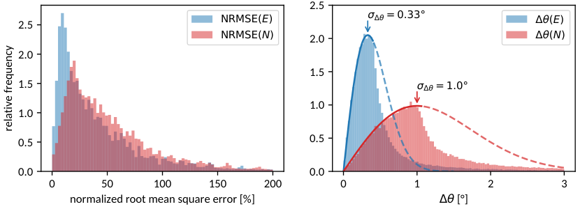
Figure 6 (left) shows normalized root mean square errors
| (12) |
of the linear tensor models (8) and (9) with respect to the noiseless input data . The statistical distribution arises both from the range of considered anisotropies and orientations. While the distributions peak at 10-20% NRMSE, values over 100% are still encountered. These deviations reflect the approximative nature of the linear tensor models.
Nevertheless, the principal orientation, which is one of the central concerns of tensor tomography, is reproduced to a typical precision of and respectively for the considered reconstruction models: Figure 6 (right) compares the eigenvectors corresponding to either the smallest (in the case of ) or largest (in the case of ) eigenvalues to the original synthesized orientation of (cf. Figure 3 for a visualization of the respective tensors and their extents). The considered eigenvector of each tensor indicating a volume element’s principal orientation is denoted , and respectively, whereby represents the ground truth. The reconstruction error (with respect to orientation) induced by the simplified models is measured by the relative angles
| (13) |
The observed orientation error distributions are compared to a normal distribution of inclination angles, which, due to integration over the azimuthal angle, takes the form
| (14) |
It can be easily shown to exhibit its maximum at in the small angle approximation . Figure 6 (right) shows to be consistent with this distribution up to the maximum value, i.e., up to its standard deviation parameter.
3.2 Eigenvalues
Figure 7 reveals fuzzy, yet almost linear relations among the normalized and sorted eigenvalues of all models despite the strong approximations involved. Due to the expected anti-correlation of the eigenvalues of with those of and (cf. the illustrating example given in Figure 3), they are sorted in reverse order prior to comparison.
Model (9) parametrized by exhibits an almost proportional relation to the original signal generating mass distribution tensor with moderate deviation from its positive definite nature. Model (8) parametrized by in contrast exhibits an inverse relation to with the spectrum of eigenvalues being notably shifted towards negative values. The mapping of eigenvalues nevertheless remains approximately linear as opposed to an actual reciprocal relation. The direct comparison of the normalized eigenspectra of and reveals – on average – a perfectly linear relation, indicating that both capture highly similar information given the present acquisition geometry (see Fig. 4). Deviations from the apparent mean curves relating the different models reflect both statistical variances among different orientations of the same volume element as well as systematic deficiencies of the simplified models. As these effects are not separable in practical applications, no further effort is made to investigate their individual contributions.
The case of one or two eigenvalues of being exactly zero corresponds to the limit of infinitely extended volume elements, causing an extreme orientation dependence and divergence of the dark-field signal according to Eq. 1 and thus also unstable (highly orientation dependent) reconstruction results in and , as can be observed in Fig. 7. This limit is expected to be only of academic relevance.

3.3 Reconstruction from three orthogonal trajectories
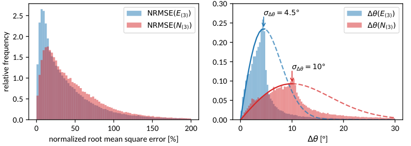

If dark-field anisotropy was actually adequately described by either of the linear models (8) or (9), three orthogonal projection trajectories (Fig. 4, blue) would fundamentally be sufficient to fully determine the respective tensor (also in a tomographic setting, cf. e.g. [3]). As such a reduced set of trajectories is highly desirable with regard to practical data acquisition, it shall therefore be briefly considered here as well. Figure 8 depicts, analog to Figs. 6–7, the relations between the considered models’ tensors. Despite the reduced set of data, which generally gives reason to expect fewer model inconsistencies, the observed distribution of root mean square errors is still qualitatively comparable to that found previously in Fig. 6. And although the visibly diffused relations between the tensors’ eigenspectra reflect a notably degraded relation between the reconstructed tensors and the original input, principal orientations are still roughly reproduced within an error margin of about 4.5° to 10°.
4 Discussion
While several proofs of concept plausibly demonstrating tomographic reconstruction of sub-resolution anisotropy based on various heuristic signal models were given in previous literature, explicit validations have been lacking so far. A central assumption explicitly or implicitly shared by all current approaches is that 3D dark-field anisotropy can be described as a function of a single orientation vector. This has been, deriving from planar dark-field anisotropy, the interferometer’s direction of sensitivity. A detailed discussion of dark-field origination given recently [6] concludes that a complete description of general dark-field anisotropy for arbitrarily oriented structures further exhibits a non-negligible dependence also on the relative orientation of the optical axis (the direction of projection). I.e., dark-field contrast will likewise vary for anisotropic structures rotating about the axis of grating sensitivity (changing their inclination with respect to the optical axis) as for the classical case of objects rotating about the optical axis (changing their orientation with respect to the interferometer’s gratings). General dark-field anisotropy is thus fundamentally a function of two orientations: the axis of interferometer sensitivity, and the axis of projection.
With regard to tensor tomography, this observation has two remarkable implications: Foremost, it obviously raises the question why the present approaches to anisotropic dark-field tomography do nevertheless produce plausible results. And as neglecting parts of the orientation dependence is apparently tolerable, this also indicates that dark-field anisotropy may likewise be approximable as a function of the optical axis, modeling variations in scattering cross section as opposed to variations in auto-correlation properties. As both effects have opposite relations with the considered structure’s extents (cf. Fig. 2 upper right), the net relation of either model to the signal generating structure is non-obvious. The purpose of the present study therefore was to systematically investigate the actual relations based on the physically motivated signal model derived and verified previously ([6]) based on the current state of knowledge on dark-field origination.
As expected, the approximative models can exhibit large root mean square errors with regard to the actual signal. When providing input data decently covering both orientation dependencies, both linear models nevertheless manage to reproduce the principal orientation of the original mass distribution tensor up to a typical accuracy of 0.33° to 1°. The normalized eigenvalues, which do encode the actual aspect ratios of anisotropic volume elements, are thereby found to be roughly linear in the normalized inverse variances of the original mass distribution (as opposed to being linear e.g. in its extents) for both models. As this is the scaling behavior expected along the axis of interferometer sensitivity, it is consistent with the observation that model (9) yields slightly better reconstruction results.
Although the true complexity of dark-field anisotropy generally mandates a rather extensive data acquisition scheme, the consequences of using only a minimal set of three circular acquisition trajectories has been explicitly considered as well. While the quantitative relation between input and reconstruction is, as expected, notably degraded, principal orientations for isolated volume elements could still be roughly recovered to 5° to 10° accuracy. As it is conjecturable that the additional influences of noise and signal superpositions (in the tomography use case) will further challenge the stability of these reconstructions in practical applications, more comprehensive acquisition schemes as considered initially are highly recommended though.
5 Conclusion
The practical feasibility of dark-field tensor volume tomography depends on the applicability of linear approximations to actual dark-field signal anisotropy, given that highly non-linear dependencies can void the ability to solve the problem of volume reconstruction from projections. Given a previously validated dark-field signal model, an exhaustive exploration of the possible parameter space for anisotropic volume elements has been performed in order to establish the general ability of approximative linear tensor models of dark-field anisotropy to recover central properties of the considered volume elements. While the reconstruction of orientation and aspect ratios is fundamentally subject to statistical variation already in the absence of signal noise, the theoretically achievable precision of 1° and better is highly encouraging with regard to quantitative tensor valued volume tomography. Although linear tensor models (in 3D space) would generally be fully determined with data from only three orthogonal projection trajectories, the data acquisition scheme must however nevertheless be guided by the true complexity of the actual dark-field anisotropy.
References
- [1] J. Arvo. III.4 – fast random rotation matrices. In D. Kirk, editor, Graphics Gems III (IBM Version), page 117–120. M. Kaufmann, 1992.
- [2] F. Bayer, S. Hu, A. Maier, T. Weber, G. Anton, T. Michel, and C. Riess. Reconstruction of scalar and vectorial components in x-ray dark-field tomography. PNAS, 111(35):12699–12704, 2014.
- [3] M. Defrise and G. T. Gullberg. 3d reconstruction of tensors and vectors. Technical Report, (LBNL-54936), 2005.
- [4] J. Dittmann, S. Zabler, and R. Hanke. Nested tomography: Application to direct ellipsoid reconstruction in anisotropic darkfield tomography. Conf. XNPIG 2017 (https://www.psi.ch/xnpig2017), page 49–50, 9 2017.
- [5] Z. Gao, M. Guizar-Sicairos, V. Lutz-Bueno, A. Schröter, M. Liebi, M. Rudin, and M. Georgiadis. High-speed tensor tomography: iterative reconstruction tensor tomography (IRTT) algorithm. Acta Cryst. A, 75(2):223–238, 2019.
- [6] J. Graetz, A. Balles, R. Hanke, and S. Zabler. Review and experimental verification of x-ray dark-field signal interpretations with respect to quantitative isotropic and anisotropic dark-field computed tomography. Phys. Med. Biol., 65(23):235017, 2020.
- [7] T. H. Jensen, M. Bech, I. Zanette, T. Weitkamp, C. David, H. Deyhle, S. Rutishauser, E. Reznikova, J. Mohr, R. Feidenhans’l, and F. Pfeiffer. Directional x-ray dark-field imaging of strongly ordered systems. Phys. Rev. B, 82(21), 2010.
- [8] J. Kim, M. Kagias, F. Marone, and M. Stampanoni. Appl. Phys. Lett., 116(13):134102, 2020.
- [9] S. K. Lynch, V. Pai, J. Auxier, A. F. Stein, E. E. Bennet, C. K. Kemble, X. Xiao, W. Lee, N. Y. Morgan, and H. Wen. Interpretation of dark-field contrast and particle-size selectivity in grating interferometers. Appl. Opt., 50(22):4310–4319, 2011.
- [10] A. Malecki, G. Potdevin, T. Biernath, E. Eggl, K. Willer, T. Lasser, J. Maisenbacher, J. Gibmeier, A. Wanner, and F. Pfeiffer. X-ray tensor tomography. EPL, 105:38002, 2014.
- [11] J. Vogel, F. Schaff, A. Fehringer, C. Jud, M. Wieczorek, F. Pfeiffer, and T. Lasser. Constrained x-ray tensor tomography reconstruction. Opt. Express, 23(12):15134–15151, 2015.
- [12] M. Wieczorek, F. Schaff, F. Pfeiffer, and T. Lasser. Anisotropic x-ray dark-field tomography: A continuous model and its discretization. Phys. Rev. Lett., 117(15):158101, 2016.
- [13] W. Yashiro, Y. Terui, K. Kawabata, and A. Momose. On the origin of visibility contrast in x-ray talbot interferometry. Opt. Express, 18(16):16890–16900, 2010.