Interpretability-Driven Sample Selection Using Self Supervised Learning For Disease Classification And Segmentation
Abstract
In supervised learning for medical image analysis, sample selection methodologies are fundamental to attain optimum system performance promptly and with minimal expert interactions (e.g. label querying in an active learning setup). In this paper we propose a novel sample selection methodology based on deep features leveraging information contained in interpretability saliency maps. In the absence of ground truth labels for informative samples, we use a novel self supervised learning based approach for training a classifier that learns to identify the most informative sample in a given batch of images. We demonstrate the benefits of the proposed approach, termed Interpretability-Driven Sample Selection (IDEAL), in an active learning setup aimed at lung disease classification and histopathology image segmentation. We analyze three different approaches to determine sample informativeness from interpretability saliency maps: (i) an observational model stemming from findings on previous uncertainty-based sample selection approaches, (ii) a radiomics-based model, and (iii) a novel data-driven self-supervised approach. We compare IDEAL to other baselines using the publicly available NIH chest X-ray dataset for lung disease classification, and a public histopathology segmentation dataset (GLaS), demonstrating the potential of using interpretability information for sample selection in active learning systems. Results show our proposed self supervised approach outperforms other approaches in selecting informative samples leading to state of the art performance with fewer samples.
Index Terms:
Interpretability, Sample Selection, Self-supervised, Lung disease classification, Histopathology segmentation.I Introduction
Supervised Deep Learning (DL) approaches trained on large datasets have shown state of the art performance [1] on medical image analysis tasks such as classification and segmentation. While DL approaches thrive on large labeled datasets, obtaining them is a challenge due to: 1) limited expert availability; 2) intensive manual effort to curate datasets (i.e. sample labeling process); and 3) paucity of images for specific disease labels leading to class imbalance.
Recent methods have taken different approaches to address the data shortage issue by using data augmentation, semi supervised learning and active learning, to name a few. Although conventional data augmentation methods relying on transformations such as rotations, random cropping, flipping, intensity rescaling, etc., artificially increase dataset size, they do not ensure incorporation of true distribution variability. Improved data augmentation via generative models has been proposed for medical image applications, where realistic synthetic images are used for data augmentation purposes [2, 3, 4, 5, 6]. While synthetic images leverage a better data augmentation process, these approaches are not designed to streamline the time-consuming data curation process needed to incorporate novel real samples. Semi-supervised learning solves the issue of limited expert availability and expert annotation work, as it leverages many unlabeled samples and a few labeled samples to train a classifier [7]. However, performance of these methods is known to be dependent upon the quality and informativeness of samples, which is not ensured by semi-supervised learning itself [8].
Active learning (AL) is an interesting learning paradigm to progressively improve a model’s performance. AL systems enable a progressive learning capability, which is ideal in clinical setups where improvements over time, based on user-feedback is desired11 1 e.g. The FDA organization has even recently mentioned their interest to adapt their regulations to facilitate exploitation of active learning. However, limited expert availability and required high clinical expertise hampers the annotation of medical images. Hence sample selection methodologies in medical image analysis applications based on supervised learning are fundamental to attain system performance promptly with minimal clinical expert interactions. We refer to this as active sample selection, where most informative unlabeled samples are selected, queried for labels, and subsequently added for further model training [9]. Additionally, we remark that active sample selection methodologies leveraging improved learnability of models is particularly important when AL-based technologies are required to swiftly adapt to potential changes of the imaging protocol, vendor type, model, etc. In the next section we review the state of the art in active sample selection.
II Prior Work on Active Sample Selection
Classical approaches for sample selection in AL methods include entropy-based sample selection [10, 11, 12, 13, 14, 15, 16, 17, 18, 19, 20], uncertainty sampling [21, 22, 23, 24, 25, 26, 27, 28, 29, 30, 31, 32], query-by-committee (QBC) [33, 34, 35, 36, 37, 38, 39, 40, 41, 42, 43] and density weighting [44, 45, 46, 47, 6, 48, 49, 50, 51, 52, 53, 54, 55]. These approaches have been used in medical imaging applications such as segmenting anatomical structures [56, 57, 58, 59, 60, 61, 62, 63, 64, 65, 66, 67] and detecting cancerous regions [68, 69, 70, 71, 72, 73, 74, 75, 76, 77, 78, 79, 80].
With the advent of deep learning based approaches, active sample selection has been investigated to accelerate learning in deep active learning setups. Different sample selection strategies have been investigated, including sample entropy [9, 81, 82, 83, 57, 84, 85, 86, 87, 88, 89, 90, 91, 92, 93, 94], model uncertainty [95, 96, 97, 98, 99, 100], Fisher information [101], and clustering [102, 103, 104, 105, 106, 107, 108, 109, 110, 111, 112, 113, 114, 115]. Proposed entropy-based approaches vary in the way the entropy metric is used. In [9, 116, 117, 118, 119, 120, 121, 122, 123, 124, 125, 126, 127], given a pool of candidate samples, the approach selects informative samples by a combination of maximal conditional entropy of the label variable given a candidate sample (sample informativeness), and mutual-information-based density estimation of samples (sample representativeness). In [81, 128, 129, 130, 131, 132, 133, 134, 135, 136, 137, 138, 139], sample entropy along with least confidence and margin sampling metrics are proposed in a general framework where least uncertain samples are pseudo-annotated with a trained oracle. In [140, 141, 142, 143, 144, 145, 146, 147, 148, 149], a query synthesis approach was proposed where a Generative Adversarial Network (GAN) synthesizes samples close to the decision boundary, which are then annotated by human experts. Inspired by this work, instead of querying annotations of synthetic samples, in [83] a GAN model is used to generate high entropy samples, which are used as proxy to find most similar real samples from a pool of candidates to be annotated by experts.
Uncertainty-based sample selection approaches are the most popular among different informative sample selection methodologies. In this paradigm, the basic idea is to select samples for which a model is most uncertain, as they contain new information for model training. In [95], a two-step sample selection approach was proposed for computer vision applications, where samples are first selected based on an uncertainty estimation derived via model bootstrapping, followed by a second selection based on a maximum set coverage similarity metric to select representative samples. This idea was followed in [100], but instead of using a two-step approach, the authors propose to combine MC dropout uncertainty-based sample selection, and sample representativeness via a borda-count approach. In addition, different from [95] where a cosine distance was used as maximum set coverage, the authors in [100] propose to measure representativeness of samples via an additional loss cost term optimizing maximum entropy of activation layers. From reported results in [100], it is however not clear how feasible it is to find a good balance between the employed cross-entropy loss (loss term for the main task) and the additional representative loss term, since in their experiments the representative loss term is assigned a very small weight.
Originally proposed in [97], and later adopted by [96, 98, 99] test-time Monte-Carlo dropout was used to estimate uncertainty of samples, and select most informative ones for label annotation. The approaches in [98] and [99] differ from [97] as they incorporate a conditional GAN based data augmentation to synthesize similar samples to those selected by the uncertainty criteria, in order to further boost the learning rate. Based on Fisher information metric, the authors in [101] propose to select samples based on an efficient low-dimensional approximation of the Fisher information metric targeting Convolutional Neural Networks. The approach however, relies on a pre-selection step based on sample uncertainty estimation, and its performance hence depends on the sensitivity level of such uncertainty-based pre-selection. In [102] sample selection is based on a representativeness approach where image patches are projected into a latent space (e.g. via a Variational Autoencoder), clustered in the latent space and sorted by their representativeness using a cosine distance maximum set coverage metric, as done in [95].
In this paper we propose a novel sample selection approach based on information derived from interpretability saliency maps. Development of interpretability methods for deep learning systems emerged from the need to leverage understanding and insights driving a model’s predictions [150]. For classification tasks, interpretability saliency maps have been proposed to yield levels of pixel attribution for a given queried class label [151, 152, 140, 153]. Interpretability saliency maps have been proposed to enhance interpretability of deep learning models via visualization of image areas driving predictions, and to perform quality assurance [154]. Different from prior works, in this paper we propose to use interpretability saliency maps in the context of selecting informative samples for active learning. Our proposition is motivated by the observation that in medical images, sample informativeness strongly relates to information about the studied pathology or condition, which in turn is target of saliency maps highlighting image areas driving a model’s prediction.
II-A Contributions
In this paper we make the following contributions:
- 1.
We propose a novel Interpretability-DrivEn sAmple seLection (IDEAL) framework. Up to our knowledge this is the first study showing how interpretability saliency maps can be used to leverage active sample selection.
- 2.
As part of the proposed framework we present results exploring three different popular approaches, featuring different levels of complexity, to design imaging features extracted from interpretability saliency maps, such as hand-crafted features (observational model), radiomics features, and deep features (data-driven model). We motivate their design and analyze their effectiveness in lung disease classification and histopathology image segmentation.
- 3.
We propose a novel end-to-end deep learning approach to extract deep features from saliency maps, which is trained to identify most informative samples in a self-supervised approach.
- 4.
We demonstrate the added value of the proposed interpretability-driven active sample selection approach by means of comparison to an standard active learning (i.e. no sample selection involved), and a state-of-the-art uncertainty-driven active learning approach, on a public database of lung-disease classification, and a publicly available dataset for histopathology segmentation.
III Methods
III-A Intuition behind IDEAL
In this section we describe the proposed IDEAL approach and its components. We start by presenting the intuition behind using interpretability methods for active sample selection, and the original observation that led us to explore this approach. From our previous studies [98, 99] using pixel-wise uncertainty maps to perform sample selection we observed a relationship between saliency and uncertainty maps, indicating the possibility of extracting information from these saliency maps to drive sample selection. Figure 1 shows two example cases of patients with pleural effusion condition, with high and low levels of uncertainty (accumulated pixel-wise uncertainties via MC Dropout). As we compared the corresponding interpretability saliency (derived from Deep Taylor method [155]) and uncertainty maps (shown in Fig. 1(b) and Fig. 1(d), respectively) and their histograms, Fig. 1(c) and 1(e), we observed that the histograms of high and low informative images are quite distinct, thus verifying the fact that high and low informative images have different values for the most salient regions. Comparing between the high informative image histograms of interpretability saliency and uncertainty maps, we observed that the highest peak of the saliency map histogram (i.e. the “primary” peak) has a higher count than the corresponding uncertainty map’s histogram “primary peak”. Additionally, the interpretability saliency map histogram “secondary peaks” have lower count than those of the uncertainty map histogram. These point to the fact that, compared to the uncertainty method, the interpretability saliency approach identifies salient regions in a more focused manner. This is beneficial when the goal is to identify the most informative saliency maps for improved classification and segmentation.
Similarly, we verified how interpretability saliency maps and uncertainty maps vary through the course of training. We selected saliency maps after adding of training samples. As shown in Figure 2, initially the saliency maps are not well defined since the classifier is not yet trained with sufficient informative samples. However, as more informative samples are being added to the training set, we observe that the saliency maps become more well defined and highlight specific regions of interest. Interestingly, we also observe that saliency maps are sharper and more detailed than uncertainty maps, suggesting an improved description of sample informativeness. The saliency map’s informative regions are concentrated and focused on important regions, while the uncertainty maps present dispersed regions. Furthermore at the same percentage of training data, interpretability saliency maps highlight qualitatively better informative regions.
These seminal observations led us to the hypothesis that saliency maps could be used as a proxy to guide an active sample selection. We investigated this hypothesis by investigating how information from saliency maps could be used to guide sample selection. We studied three different approaches to extract information: starting from a simple histogram feature (stemming from our initial observation), followed by a radiomics-based approach, and finally, an end-to-end deep learning based approach cast as a self-supervised learning problem. In the following sections we describe the components of the proposed IDEAL approach, including the different investigated information extraction approaches.
 |
 |
 |
 |
 |
 |
 |
 |
 |
 |
 |
 | |
| (a) | (b) | (c) | (d) | (e) | (f) |
III-B Main components of IDEAL
Figure 3 depicts a general pipeline of the proposed IDEAL approach. Given unlabeled testing samples (i.e. sample pool), and an associated deep learning classification model (e.g. DenseNet) trained iteratively during active learning, an interpretability saliency map generator is used to produce saliency maps, from which a sample informativeness score (IDEAL Scoring) is calculated to rank pool samples by their informativeness. The IDEAL scoring can be produced in different ways, depending on how the information from the saliency maps is distilled to produce a ranking score for each pool sample. In this study we investigated three different ways of extracting information and scoring samples, which are presented in order of complexity: (i) From our original observation, a single feature extracted from the histogram of saliency maps (Fig. 1(c)) is used to derive the IDEAL scoring, (ii) Multivariable radiomics features are extracted and combined into single IDEAL scores, and (iii) Our proposed novel Deep features extracted and used within a self-supervised approach to score informative samples.
In the following we describe each component in detail and in relation to the clinical problem of automating lung disease classification and histopathology segmentation, as well as baseline methods used to benchmark the proposed IDEAL approach.

III-C Classification model
The classification model is not per se a component of the IDEAL approach but rather an input its calculations are based on. We present it here to facilitate the presentations and descriptions of the data workflow, as presented in Fig. 3. Any robust classification model can be used as the approach is not restricted to particular architectures. For lung disease classification from X-ray images, we experimented with different models namely, DenseNet-121 [156],ResNet-50 [157] and VGG16 [158], and found the DenseNet-121 architecture to perform the best. We denote as , the DenseNet-121 model, and point the reader to section IV-C, for further implementation details of the trained model. For the histopathology image segmentation task we used a DenseNet-121 classifier of the histopathology images (benign vs. malign), as a proxy of informativeness for the main task of image segmentation. This was motivated by multi-task learning where tasks are typically intertwined, and the availability of interpretability approaches for classification tasks. As shown in the results section, we show that this approach is effective in the segmentation task as well.
III-D Interpretability Saliency Map Generator
Image-specific saliency maps operate under the the basic principle of highlighting areas of an image that drive the prediction of a model. The importance of these areas can be obtained by investigating the flow of the gradients of a DL model calculated from the model’s output to the input image, or by analyzing the effect of a pixel (or region) to the output when that pixel (or region) is perturbed. This type of visualization facilitates interpretability of a model but also serves as a confirmatory tool to check that machine-based decisions align with common domain knowledge [150]. As mentioned, differently from previous works in interpretability, we aim here to employ saliency maps to perform active sample selection. To generate interpretability saliency maps we use the iNNvestigate library [155] 22 2 https://github.com/albermax/innvestigate, which implements several known interpretability approaches. We employ Deep Taylor, a known interpretability approach to generate saliency maps, due to its ability to highlight informative regions while yielding minimal importance to other regions. Deep Taylor operates similarly as other interpretability approaches by decomposing back-propagation gradients, of the studied model, into layer-wise relevance maps of individual cell activations, as a function of a queried input sample and class label (e.g. disease class)[159].
III-E IDEAL Sample Informativeness Score
In this section we formalize the definition of the IDEAL sample scoring. Given a test image , a prediction model being updated via active learning, and the corresponding saliency map , we map the saliency map into a sample informativeness score, termed IDEAL score as:
| (1) |
The function can have different forms, depending on the way the information is extracted from the saliency map and converted into an informative sample score. We present results investigating three different approaches, described in further detail below.
The IDEAL scores obtained for the set of testing samples are sorted in decreasing order and the top-n ranked samples are chosen for expert label querying and added to the next active learning cycle. The complete IDEAL process is summarized in Algorithm 1. In Algorithm 1 the model can be a pretrained network or, as in our experiments, trained with a small part of the training dataset (e.g. 10% of training).
We now describe in detail each of the three studied feature extractor approaches:
III-E1 Single Hand-crafted Feature - Kurtosis
This first approach is motivated by the observation made from the histograms between high and low uncertainty samples, Figure 1. As operator in Equation 1, we defined , with and corresponding to the histogram and kurtosis operators, respectively. Consequently, and based on our observations, informative samples are associated to larger kurtosis values and sorted accordingly to select informative ones. In the results section, this approach is referred to as Kurtosis.
III-E2 Multivariate Radiomics Features
As second approach, we used the PyRadiomics package [160] to extract different radiomics features from the saliency maps. Owing to the large number of potential features we employ a feature selection strategy. PyRadiomics has 8 feature categories. We trained random forest (RF) classifiers to predict the image’s disease label using each feature category. Based on the in-built information gain of the RF model, we identified the best performing categories as: “First Order Statistics” ( features), “Gray Level Co-occurrence Matrix (GLCM)” (24 features), and “Shape Based (2D)” ( features). The final features for each category is identified by performing an exhaustive search over all possible feature combinations and using it to predict disease labels with a RF classifier. The final features are summarized in Table I.
In order to combine extracted selected radiomics features for ranking, we rank different metrics based on the Borda count, which has been used before for ranking informative samples [100]. With Borda count samples are ranked for each metric, and samples are selected based on the best combined rank as:
| (2) |
where denotes the pyradiomic feature calculated on image .
In the results section, this approach is referred to as PyRad_category, with category being one of the following {1st-order, GLCM, 2DShape}.
| Feature Type | Comments |
|---|---|
| Kurtosis | Obtained from histogram of the intensity distribution |
| Radiomics- | Initial features. Exhaustive search on |
| First Order | combinations. best features - ‘Kurtosis’, ‘Skewness’, |
| ‘Entropy’ and ‘Total Energy’. | |
| Radiomics- | Initial features. Exhaustive search on |
| GLCM | combinations. best features -‘Sum Entropy’,‘Inverse |
| Difference Normalized’,‘Difference Entropy’ and | |
| ‘Maximal Correlation Coefficient’. | |
| Radiomics- | Initial features. Exhaustive search on |
| Shape | combinations. best features -‘Sphericity’, ‘Spherical |
| Disproportion’, and‘Elongation’ | |
| Deep Saliency | Ordinal Clustering of latent feature vector |
| Features | followed by Self-Supervised step. Details in text. |
III-E3 Deep Saliency Features: Ordinal Clustering And Self Supervised Learning For Informative Sample Selection
In this section we present the third and more advanced approach. We propose a novel approach that uses deep features extracted from an autoencoder and self supervised learning based ordinal clustering of informative samples.
The goal in self-supervised learning is to identify a suitable self supervision task (or pretext task) that provides additional knowledge (in the form of network weights) to successfully train a model to solve the main task. Some common pretext tasks include for example, estimating relative position of patches [161], simulated deformation [45], segmentation [46], aggregation learning [47], local context [162], and colour [163]. Additionally, exemplar learning has been proposed as a self-supervised learning strategy [164] where the task is to classify each data instance into a unique class.
Given a set of candidate pool samples, saliency maps are generated and, as first step, an auto encoder is trained to reconstruct them. The output of the encoding stage is a dimensional latent feature vector representation (referred to as Deep Saliency Features), which is used as input for the next stage of ranking them. In order to discriminate informative samples from Deep Saliency Features, and in the absence of information to distill which Deep Saliency Features are associated to sample informativeness, we cast the problem as a self supervised learning approach to assign informativeness labels to saliency maps. Figure 5 depicts the proposed self supervised learning approach, which is also explained in Algorithm 2. It consists of the following steps:
- 1.
Extracted latent feature vector representations are clustered using an ordinal cluster approach into clusters.
- 2.
Identify most representative sample of each cluster via measuring the closest sample to its centroid using L2 distance between extracted latent feature vectors.
- 3.
Query labels of the most representative sample per cluster (e.g. queries)
- 4.
Add the corresponding original image to the training set, and determine the change in AUC values () for a fixed validation set (independent of the training set). Rank samples according to decreasing .
- 5.
Identify cluster whose representative image yields maximum positive AUC on validation set.
- (a)
Select this cluster as most informative
- (b)
Label each cluster as where is most informative cluster and denotes least informative cluster.
- (c)
Ranking and queried labels for each representative sample are propagated to all samples within each cluster.
- (a)
- 6.
Use labelled samples from the previous step, and their corresponding deep saliency features to train a random forest classifier. In order to efficiently train the random forest classifier as new samples are selected, we use online random forests [165], which performs incremental training of the RF using the previously trained RF as a starting point. The saliency map is classified into one out of possible levels of informativeness. Use (Algorithm 2) to rank new (test) samples based on informativeness.
Figure 4 shows the t-SNE plots of features from samples belonging to different informativeness clusters, where ‘Cluster 1’ denotes the most informative image cluster while ‘Cluster 10’ denotes the least informative cluster. We see a clear separation between different informativeness clusters. There is some overlap of neighboring clusters, which is due to the similar feature characteristics of similarly informative images/samples.
The choice of was to strike a balance between level of granularity and avoid clusters with too few or no samples. If is too high then we have to increase the batch size (from 32 to higher) to ensure sufficient samples in each cluster for accurately determining a representative vector. However, increased batch size leads to higher computation cost and poses challenges during training. If is too low then we lose granularity of informativeness rankings. For example, if then samples with different levels of informativeness will be in one cluster and make it difficult to train a reliable classifier to predict informativeness. Thus gives the best tradeoff between these two considerations.
 |
The proposed ordinal clustering and self supervised learning approach for informative sample selection leverages feature extraction information using modern deep learning technologies. This comes at the cost of a minimal label expert querying of representative samples (i.e. number of cluster , which based on our experience and the results obtained, yields a good trade-off for clinical utilization.
In the results section this approach is referred to as Deep Features. In the next section we present results obtained with the proposed and baseline approaches, along with several ablation experiments aiming at leveraging further insights and confirmatory evidence on the benefits of the proposed IDEAL approach.
 |
IV Baseline Methods For Comparison
In this section we describe the baseline methods used for comparison purposes.
IV-A Standard Active Learning
As first baseline we considered a standard active learning framework where no sample selection is considered. In this setup, given a set of testing samples, a subset of samples are randomly chosen for label querying and active learning training. It is worth noting, that in clinical practice the number of samples reflects the amount of user interaction needed to incorporate new samples into the next cycle of active learning, and hence it needs to be kept as low as possible. In the results section we refer to this approach as Random.
IV-B Uncertainty-driven sample selection
This corresponds to our second baseline. As proposed in [98, 99], uncertainty estimation can be used as a metric of sample informativeness for active learning. Given the deep learning model used for disease classification, mapping an input image , to a unary output , the predictive uncertainty for pixel is approximated using:
| (3) |
is the model’s output for the predicted variance for pixel , and being a set of sampled outputs.
Similarly as for the other compared approaches, the obtained uncertainty estimates are sorted from high to low uncertainty, and the top-n samples are chosen for label querying, and added to the next active learning cycle. In the results section we refer to this approach as Uncertainty.
IV-C Implementation details
Our method was implemented in TensorFlow. We trained DenseNet-121 [166] on NIH ChestXray14 dataset [167], and for the histopathology datasets. We used Adam [168] with , , batch normalization, binary cross entropy loss, learning rate , update iterations and early stopping based on the validation accuracy. The architecture and trained parameters were kept constant across compared approaches. Training and test was performed on a NVIDIA Titan X GPU having GB RAM. Images are fed into the network with size pixels.
We employed 4-fold data augmentation (i.e. each sample augmented 4 times) using simple random combinations of rotations (), translations ( pixels in horizontal and vertical directions), and isotropic scaling ( scaling factors). For generation of interpretability saliency maps, we used default parameters of the iNNvestigate implementation of Deep Taylor [155]. For uncertainty estimation we used a total of dropout samples with dropout distributed across all layers [169]. During active learning the batch size for our experiments was set to .
As shown in Figure 5 the encoder stage has 3 layers of neurons. The output is a dimensional latent feature vector which is fed to the decoding stage. The output is supposed to reconstruct the original input using the mean square error loss.
V Results and Discussion
V-A Dataset Description
As use-case applications we applied and analyzed the proposed IDEAL method and baseline approaches on two tasks: Lung disease classification and histopathology segmentation. Classification Dataset: For lung disease classification we adopted the NIH ChestXray14 dataset [167] having expert-annotated frontal-view X-rays from unique patients.
Segmentation Dataset: For histopathology segmentation we used the public GLAS digital histopathology image dataset [170] that has manual segmentation maps of glands in stained images derived from histological sections from different patients with stage or colorectal adenocarcinoma. The slides were digitized with a Zeiss MIRAX MIDI Slide Scanner having pixel resolution of m. The WSIs were rescaled to a pixel resolution of m (equivalent to magnification). visual fields from malignant and benign areas from the WSIs were selected to cover a wide variety of tissues. An expert pathologist graded each visual field as either ‘benign’ or ‘malignant’. Further details of the dataset can be found in [170].
For the lung classification task, we chose pleural effusion as target condition of a classification model, since it is clinically well defined and among the most important lung disease conditions requiring effective computer assisted diagnosis solutions. We selected patient images from the NIH dataset with pleural effusion, which are free of artefacts (e.g. incomplete lung regions) and which can lead to accurate visual assessment by an expert radiologist. As sanity check, we additionally asked our expert chest radiologist to inspect and confirm the training and testing cases, corresponding labels, as well as the corresponding interpretability saliency maps.
For each task, the dataset was split into training (), validation () and test (), at the patient level such that all images from one patient are in a single fold.
V-B Results for IDEAL and Baseline approaches
In this section we present the main results obtained by the proposed IDEAL approach, and the baselines described in section IV. As evaluation metrics we adopted the Area Under the Curve (AUC), as typically done for active sample selection studies in classification tasks, and the Dice coefficient for the segmentation task. For both tasks, we assessed the metrics for different methods at every increment of training data. Note that we perform the training from scratch using data augmentation and do not use any pre-trained network weights.
For readability purposes, we split the presentation of our main results in Figure 6 in two plots: Figure 6(a) shows results for baselines (Uncertainty and Random), and approaches of Kurtosis and best Radiomics (PyRad-1st-order), and Figure 6(b), where we present results for Deep Saliency Features, and the best result from Figure 6(a) using Radiomics (PyRad-1st-order), which is shown as a dotted line to provide a performance comparison reference with Figure 6(a).
For completeness, we additionally include in Fig. 6(b) other radiomics-based results yielded via GLCM texture features, and 2D-shape based features. On both plots in Fig. 6, results with a fully-supervised model (FSL, AUC=)) are also included (horizontal lines in Fig. 6(a) and (b)).
From Fig. 6(a) we observe that, except for Random-based sample selection, all approaches outperform the fully-supervised learning model. Moreover, IDEAL approaches based on Kurtosis and Radiomics outperform uncertainty-based sample selection. Additionally, the uncertainty-based approach required of the training data to surpass FSL, which was surpassed at a much lower value for IDEAL approaches: Kurtosis: , and PyRad: . We remark that this finding aligns with other similar reports, [83, 95, 101], but its exploration goes beyond the scope of this study.
Amongst the different Radiomics based features, best AUC was attained with First-Order features, while GLCM performed poorly, followed by 2D-Shape. We attribute this lower performance of GLCM and 2D-shape based features to a combination of an absence of rich texture and shape information of saliency maps, as well as the difficulty to reliably extract shape parameters with pyradiomics (e.g. finding an appropriate parameterization of threshold values to binarize saliency maps before extracting shape information).
As shown in Fig. 6(b), the third approach, based on Deep Saliency Features in combination with the proposed self-supervised ordinal clustering, yielded the best results, outperforming all other approaches in terms of learning rate and final attainable accuracy. Using IDEAL with Deep Saliency Features, enables the approach to attain same performance as the fully-supervised model at only (versus using uncertainty-based sample selection), with best final performance at . We highlight these results in light of the importance of minimizing expert annotations in the clinical routine while targeting high accuracy levels.
The AUC values were derived from an average of runs and the statistical significance with respect to Deep Saliency Features was calculated using a paired test. The final AUC values and the corresponding values for different methods are as follows: 1) FSL-; 2) ‘Deep Saliency Features’-; 3) Kurtosis- ; 4) Uncertainty -; 5) PyRad-1st-Order - ; 6) PyRad-GLCM -; 7) PyRad-2DShape- .
 |
| (a) |
 |
| (b) |
V-C Relationship Between Batch Size And Interaction Cost
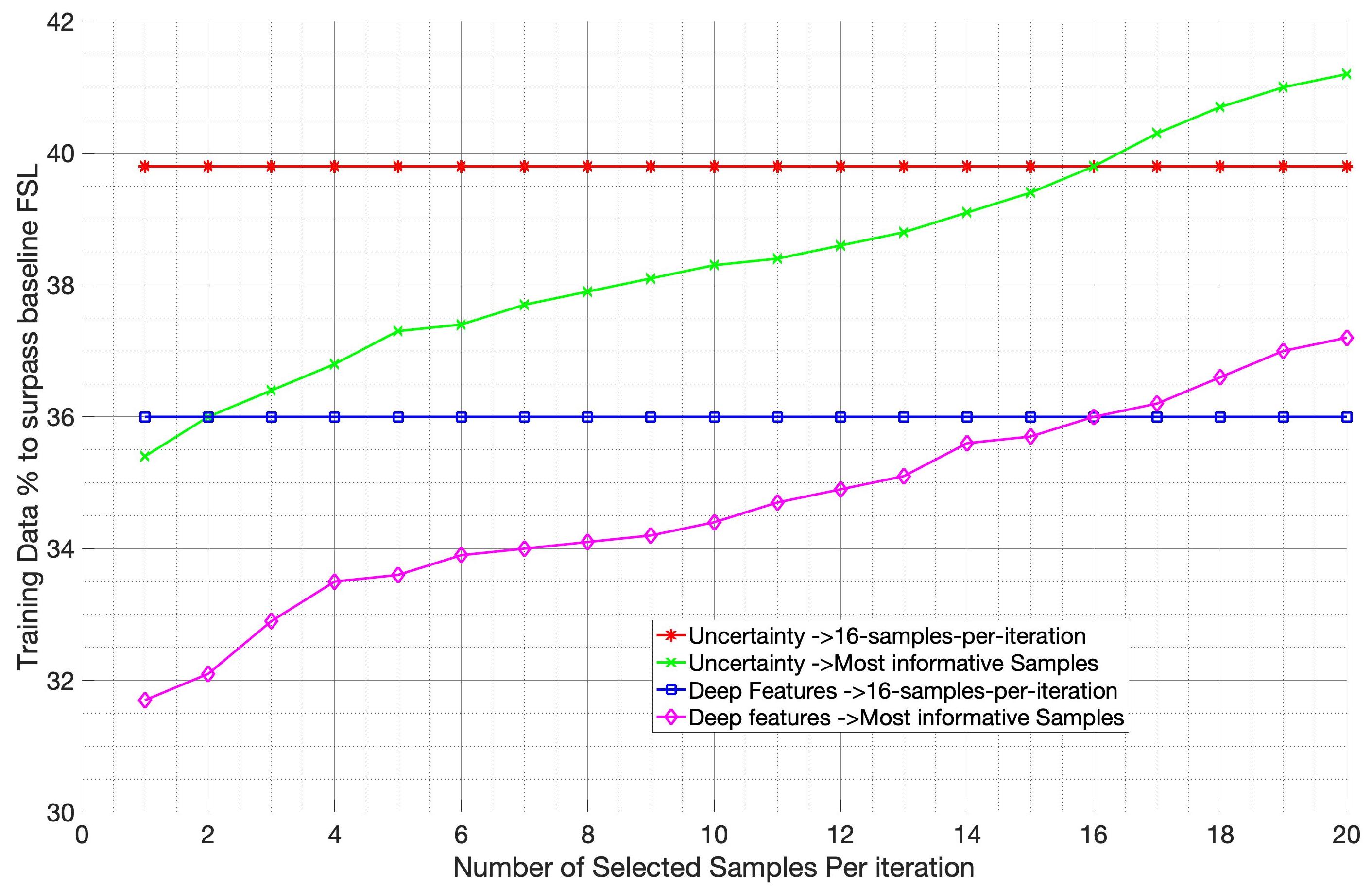
We analyzed the interplay between varying the number of queried samples (line 8 in Algorithm 1)), and the total number of training iterations required for the active learning system. For this experiment we used the classification task. As reference we used the performance of the fully-supervised model and measured the number of queried samples and training iterations needed by IDEAL to surpass the performance of the fully-supervised model. Figure 7 (a) shows that with reduced number of samples per batch the system can surpass FSL with fewer samples. During the initial phase of fixed-batch size training, queried samples within a single batch might indeed be assessed as being informative, but redundant as they share similar characteristics, leading to the effect that a higher percentage of training dataset is needed to surpass the performance of the fully-supervised model. In the extreme case of selecting one sample per iteration the system will always choose the most informative sample and there will be no redundancy in subsequent sample selections.
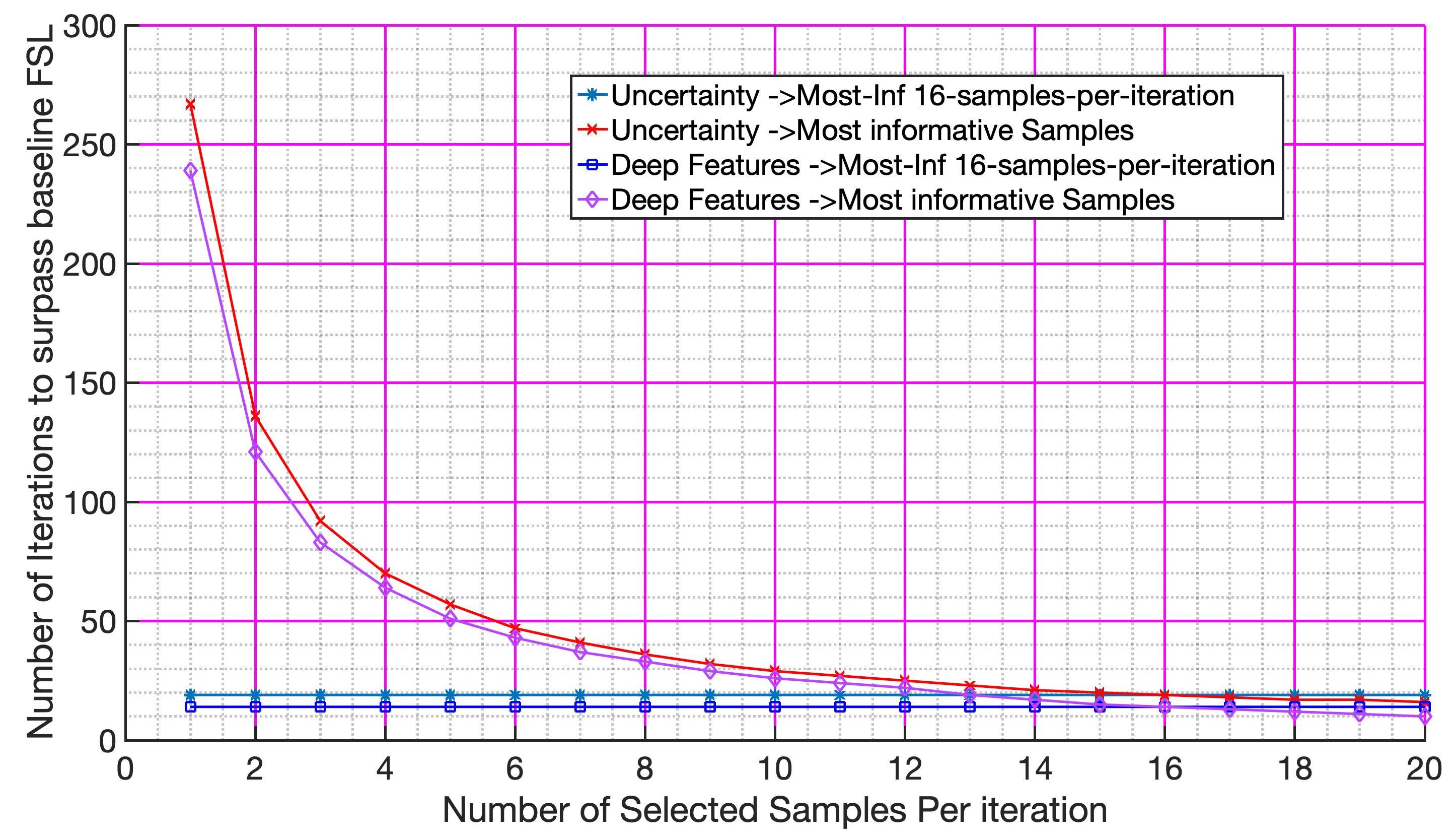
However, as shown in Figure 7 (b), for both IDEAL and uncertainty-based sample selection approaches, a reduction in the number of selected samples per iteration comes at the cost of an exponential increase in the number of training iterations. However, IDEAL requires fewer iterations (on average 10 fewer iterations) than an uncertainty-based sample selection approach.
This also connects with the phenomenon shown in Figure 6 where the baselines based on sample informativeness outperform the fully-supervised model at lower number of training samples. This observation can also be linked to the known phenomenon of influential observations, where samples (observations) have greater influence during the initial training stages than in later ones. We remark that this phenomenon has been reported by others [83, 101, 95].
Although fewer queried samples per batch can lead to lower percentages of training dataset needed to attain a given performance (compared to using larger batches), there is the higher cost of successive retraining of the model. This can be computationally prohibitive depending on the model size, available resources, etc. For the studied use-case, we found that a batch size of queried samples per iteration could provide in practice a good trade-off between queried expert labeling and model retraining.
An interesting strategy for sample selection could be that of selecting fewer samples per iteration in the initial learning stages, to then increase the number of selected samples when the classifier has reached a certain performance level. This can potentially ensure that the classifier observes diverse samples in the initial stages while being computationally efficient to reach optimal performance.
 |
| (a) |
 |
| (b) |
V-D Ablation Studies
We performed two ablation experiments to (i) analyze the effect of choosing the least informative samples (instead of the most informative) on the learning curves, and (ii) utilize the input images, instead of the interpretability saliency maps for feature extraction. For these experiments we used the lung disease classification task.
For the first ablation experiment, Figure 8 (a) shows the classification performance when using the least informative samples ( marked as “-Reversed”). As expected, we observe a very slow increase in the learning rate. Nevertheless, the least informative “Deep Features” select better quality features and hence outperform other methods. Similarly, we observed that around of training, the learning rate increases, since the remaining samples are actually the most informative samples in the dataset. This experiment confirms the importance of selecting informative samples.
Figure 8 (b) shows the AUC curves when applying the different IDEAL based methods on the original images instead of the saliency maps (marked as “-Image”). The performance of each approach is lower than the corresponding one when extracting features from the saliency maps. We attribute this to our intuition that saliency maps highlight information regarding the pathology, which is in turn the target of the classification model being explained. In contrast, the X-ray image includes other sources of information, including the overall anatomy, that is of much lower relevance for the trained model.
 |
| (a) |
 |
| (b) |
V-E Sample Selection Performance when Switching Datasets
We assessed the proposed approach on a scenario where, after initial training with one dataset, the sample selection method may be used on a different new dataset in a clinical scenario (e.g. change of imaging vendor). To simulate this situation we used the the ChexPert Dataset [171], which contains chest radiographs of patients as our second dataset. The initial trained model was trained on the NIH ChestXray14 dataset, as described previously. We selected patient images from the ChexPert dataset having pleural effusion. The dataset was split into training (), validation () and test (), at the patient level such that all images from one patient are in a single fold.
To simulate this situation we started training with dataset 1 (e.g. NIH) and at mid way of training () we switched to dataset 2 (e.g. the CheXpert dataset [171]). Figure 9 shows the AUC curves for different IDEAL approaches. From this experiment we observe that the performance for both IDEAL and Uncertainty-based methods improved when switching to the CheXpert dataset, compared to the reference plots of Figure 6 (shown as dotted lines in Figure 9). The improvement can be attributed to the better quality of the CheXpert dataset (due to higher image resolution and higher SNR). This observation is also supported by the results in [156] where the AUC values on the CheXpert dataset are higher than those reported for the NIH dataset for the same disease label.
 |
| (a) |
V-F Results For Semantic Segmentation
For the task of histopathology image segmentation, the principle of informative sample selection holds true for segmentation as the segmentation network will benefit by learning from diverse and informative images. The motivation is to select the most informative images and their masks for training such that maximum performance gain can be achieved with minimal annotation cost. In order to derive saliency maps for the segmentation task, a classifier (DenseNet-121) for histopathology images (that identifies images as “benign” and “malign”) was used as proxy to derive interpretability features and guide sample selection.
Similar to the approach for classification we identify informative samples based on classification labels and use the images with their masks for segmentation. A standard UNet [172] is trained to perform segmentation, and the corresponding Dice metric values for every increase in dataset size are shown in Figure 10. The UNet has convolution blocks followed by downsampling in the contracting path, followed by upsampling stages in the expansion stage. Each convolution block in the contracting path has convolution steps consisting of filters with ReLU activation followed by batch normalization and downsampling. In the expansion path each deconvolution layer has stride followed by concatenation with the corresponding cropped feature map from the contracting path. It is followed by two convolution layers with ReLU activation function (with batch normalization).
In the initial stages when the segmentation network encounters new samples, the rate of increase of Dice metric is high but flattens in the later stages. Similar to the results for pleural effusion classification we also observed that sample selection outperforms fully supervised learning based segmentation.
 |
| (a) |
V-G Performance on Simulated Noise
In an attempt to simulate low informativeness we added simulated noise of and different . Figure 11 shows the AUC values for . The performance for ‘Deep-Features’ without noise is shown as a dotted line for reference. With added noise the performance of all feature extraction methods degrade. However the deep features obtained using self supervision still perform the best and are more robust than other methods.
 |
V-H Results on Pneumonia
We additionally tested on a second lung condition to check generalization of the findings on a different condition. Figure 12 shows AUC plot for pneumonia. We used images from different patients having pneumonia and the dataset was split into training (), validation () and test (), at the patient level such that all images from one patient are in a single fold. The characteristics of the different methods are similar to their pleural effusion counterpart in Figure 6. The results show that sample selection based on informativeness improves classifier performance for multiple diseases, and our proposed deep features do better than conventional feature extraction methods.
 |
V-I Influence of Saliency Map Computation
In this section we show results when using a different saliency map extraction method such as Grad-CAM [173] to check for generalization of the findings when using a different interpretability approach.
Figure 13 shows the saliency map visualizations using Deep Taylor and Grad-CAM for high-informative and low-informative images. In the case of high-informative images both approaches identify similar areas as salient. However, for low informative image (bottom row) the localized regions are quite different. Deep Taylor method highlights regions near the lung but the Grad-CAM method tend to localize an area beyond the lung region where there is no anatomy of interest. This justifies our choice of using Deep Taylor approach for generating saliency maps. Moreover, Figure 14 shows AUC plots using Grad-CAM generated saliency maps. The trends are similar to Deep Taylor generated maps, showing the superiority of proposed approach over the baselines. However in comparison with Deep Taylor, the AUC values yield via Grad-CAM are lower for each of the corresponding feature extraction methods (see Figure 6). The plots also quantify the superior performance via Deep Taylor saliency maps, and point to the differences in interpretability maps studied in the literature [154, 150].
 |
 |
 |
 |
 |
 |
| (a) | (b) | (c) |
 |
V-J Similarity Analysis Of Selected Images
V-J1 Quality of Unlabeled Image Rankings
We analyzed the rankings produced by the different sample selection approaches. To this end we used the normalized Discounted Cumulative Gain (nDCG) to compare rankings [174]. The nDCG is defined as
| (4) |
where DCG is Discounted Cumulative Gain and is defined as
| (5) |
where represents the number of retrieved images considered. Relevance values () were assigned from 1 to 5.5, 1 being the least similar image according to the reference ranking and 5.5 the most similar one (i.e., the relevance of two contiguous positions differs by 0.5).
The reference ranking was set as the Deep Features, which was compared with the informativeness ranking provided by the other methods. Figure 15 shows the comparison results, where higher values indicate better agreement. Particularly, the highest agreement was found between ‘Deep Features’ and features. The plots support our previous observations (e.g., Figure 6) where showed to have the closest performance to ‘Deep Features’.
 |
V-J2 Analysis of selected samples across methods
We further analyzed the number of common samples chosen by the different feature types of the IDEAL approach. Figure 16 shows the percentage of common samples chosen for the following informative sample selection approaches: 1) All methods - Kurtosis, PyRad1st-Order and Deep Features; 2) ‘Deep Features vs. Kurtosis’- the common informative samples chosen by our proposed Deep Features and Kurtosis; 3) ‘Deep Features vs. Uncertainty’- the common informative samples chosen by our proposed Deep Features and Uncertainty; 4) ‘Kurtosis vs. Uncertainty’- the common informative samples chosen by Kurtosis and Uncertainty; 5) ‘Deep Features vs. PyRad1st-Order’- the common informative samples chosen by Deep Features and PyRad1st-Order. We observed from Figure 16 that during the initial stages the percentage of common samples is higher and then decreases subsequently. This is explained as in the initial stages there are more informative samples to choose from and hence a larger overlap of common samples appears. As the training progresses, the subsequent chosen informative samples tend to be different depending upon the accuracy of the classifier.
 |
V-K Analysis Of Clinician Workload
We engaged an experienced lung radiologist, with over 15 years of experience in analysing chest X-ray images, to assess differences when analyzing different levels of informative images, as selected by our method. We selected images having pleural effusion - split in two groups of high informative and low informative images. The level of informativeness was chosen by our algorithm using Deep Features. The clinician was blinded to the informativeness label as well as to the image’s disease label, and was asked to diagnose the images by recording the time taken for each diagnosis.
On average the clinician spent seconds on each of the low informative images and he correctly diagnosed of the cases. For high informative images he spent on average seconds on each image and correctly diagnosed of the cases. The clinician spent an extra time (i.e. 0.62 seconds) time to diagnose the high informative images, and commented on the higher subtlety of the diagnosis as well as other factors such as fluid overload and not congestive heart failure, increasing the complexity. Hence, the time difference between diagnosing low and highly informative samples is negligible for an expert. The proposed approach requires of training samples to attain the same performance as a fully-supervised approach (Figure 6(b)) compared to for the Uncertainty based baseline (Figure 6(a). Our automated algorithm can classify an image in seconds. In light of these findings assessing clinician’s workload and learning rates we conclude on the time benefits the proposed IDEAL approach can bring to clinicians. We also observed a slightly higher percentage of accurately diagnosed cases for high informative images. The higher information content of the images leads to a better diagnosis accuracy which is along expected lines. The results show that the images chosen as highly informative by our method are indeed so as supported by the high analysis time and higher diagnostic accuracy by clinicians. Thus our algorithm can effectively contribute to reducing clinician workload.
VI Conclusions
In this work we have presented results of an interpretability-driven active sample selection (IDEAL). IDEAL uses information from interpretability saliency maps to select informative samples for active learning. We propose a novel self supervised approach using deep features and ordinal clustering to determine the most informative sample. Results on publicly available datasets for lung pleural effusion and pneumonia disease classification and on histopathology image segmentation, show that the proposed IDEAL self supervised deep features outperform other methods in selecting the most informative samples for an effective active learning system. Additionally, the use of interpretability saliency maps provides experts with a mechanism to audit and monitor the active learning process, which we believe is an important added value of the proposed IDEAL approach.
As presented here, we believe interpretability approaches not only can be used to enhance understanding of model’s predictions, but also to assist and provide further information of value in other areas of model performance, training and evaluation. In this regards, an area of potential research relates to the possibility of linking interpretability approaches with recent work on minimization of stochastic gradient to improve training of deep neural networks [175, 176].
VII Acknowledgements
This work was supported by the Swiss National Foundation grant number 198388, and Innosuisse grant number 31274.1.
-A Training, Validation and Testing Loss Error Plots
Figure 17 shows the variation of training, validation and test error values with increasing number of epochs when training the model on pleural effusion images. The training and validation losses are at similar values indicating there is no overfitting to the training set. The test error is expectedly higher but not significantly when compared to the training loss.
 |
References
- [1] N. Tajbakhsh, J. Shin, S. Gurudu, R. T. Hurst, C. Kendall, M. Gotway, and J. Liang., “Convolutional neural networks for medical image analysis: Full training or fine tuning?.” IEEE Trans. Med. Imag., vol. 35, no. 5, pp. 1299–1312, 2016.
- [2] C. Fu, S. Lee, D. Joon Ho, S. Han, P. Salama, K. W. Dunn, and E. J. Delp, “Three dimensional fluorescence microscopy image synthesis and segmentation,” in Proceedings of the IEEE Conference on Computer Vision and Pattern Recognition Workshops, 2018, pp. 2221–2229.
- [3] D. Jin, Z. Xu, Y. Tang, A. P. Harrison, and D. J. Mollura, “Ct-realistic lung nodule simulation from 3d conditional generative adversarial networks for robust lung segmentation,” in International Conference on Medical Image Computing and Computer-Assisted Intervention. Springer, 2018, pp. 732–740.
- [4] C. Bowles, L. Chen, R. Guerrero, P. Bentley, R. Gunn, A. Hammers, D. A. Dickie, M. V. Hernández, J. Wardlaw, and D. Rueckert, “Gan augmentation: Augmenting training data using generative adversarial networks,” arXiv preprint arXiv:1810.10863, 2018.
- [5] X. Yi, E. Walia, and P. Babyn, “Generative adversarial network in medical imaging: A review,” Medical image analysis, vol. 58, p. 101552, 2019.
- [6] D. Mahapatra, B. Bozorgtabar, and L. Shao, “Pathological retinal region segmentation from oct images using geometric relation based augmentation,” in In Proc. IEEE CVPR, 2020, pp. 9611–9620.
- [7] V. Cheplygina, M. de Bruijne, and J. P. Pluim, “Not-so-supervised: a survey of semi-supervised, multi-instance, and transfer learning in medical image analysis,” Medical image analysis, vol. 54, pp. 280–296, 2019.
- [8] N. Tajbakhsh, L. Jeyaseelan, Q. Li, J. N. Chiang, Z. Wu, and X. Ding, “Embracing imperfect datasets: A review of deep learning solutions for medical image segmentation,” Medical Image Analysis, p. 101693, 2020.
- [9] X. Li and Y. Guo, “Adaptive active learning for image classification,” in Proc. CVPR, 2013.
- [10] A. Holub, P. Perona, and M. C. Burl, “Entropy-based active learning for object recognition,” in IEEE CVPR, 2008, pp. 1–8.
- [11] S. Kuanar, D. Mahapatra, M. Bilas, and K. Rao, “Multi-path dilated convolution network for haze and glow removal in night time images,” The Visual Computer, pp. 1–14, 2021.
- [12] D. Mahapatra, A. Poellinger, L. Shao, and M. Reyes, “Interpretability-driven sample selection using self supervised learning for disease classification and segmentation,” IEEE TMI, pp. 1–15, 2021.
- [13] L. Ju, X. Wang, X. Zhao, H. Lu, D. Mahapatra, P. Bonnington, and Z. Ge, “Synergic adversarial label learning for grading retinal diseases via knowledge distillation and multi-task learning,” IEEE JBHI, vol. 100, pp. 1–14, 2020.
- [14] B. Bozorgtabar, D. Mahapatra, I. Zlobec, T. Rau, and J. Thiran, “Computational pathology.” Frontiers in Medicine, vol. 7, 2020.
- [15] D. Mahapatra and Z. Ge, “Training data independent image registration using generative adversarial networks and domain adaptation.” Pattern Recognition, vol. 100, pp. 1–14, 2020.
- [16] Z. Ge, D. Mahapatra, X. Chang, Z. Chen, L. Chi, and H. Lu, “Improving multi-label chest x-ray disease diagnosis by exploiting disease and health labels dependencies.” In press Multimedia Tools and Application, pp. 1–14, 2019.
- [17] B. Bozorgtabar, D. Mahapatra, and J.-P. Thiran, “Exprada: Adversarial domain adaptation for facial expression analysis.” In Press Pattern Recognition, vol. 100, pp. 15–28, 2020.
- [18] B. Bozorgtabar, D. Mahapatra, H. von Teng, A. Pollinger, L. Ebner, J.-P. Thiran, and M. Reyes, “Informative sample generation using class aware generative adversarial networks for classification of chest xrays.” Computer Vision and Image Understanding, vol. 184, pp. 57–65, 2019.
- [19] D. Mahapatra, B. Bozorgtabar, and R. Garnavi, “Image super-resolution using progressive generative adversarial networks for medical image analysis.” Computerized Medical Imaging and Graphics, vol. 71, pp. 30–39, 2019.
- [20] D. Mahapatra, “Semi-supervised learning and graph cuts for consensus based medical image segmentation.” Pattern Recognition, vol. 63, no. 1, pp. 700–709, 2017.
- [21] D. Lewis and J. Catlett, “Heterogenous uncertainty sampling for supervised learning,” in Proc. ICML, 1994, pp. 148–156.
- [22] J. Zilly, J. Buhmann, and D. Mahapatra, “Glaucoma detection using entropy sampling and ensemble learning for automatic optic cup and disc segmentation.” In Press Computerized Medical Imaging and Graphics, vol. 55, no. 1, pp. 28–41, 2017.
- [23] D. Mahapatra, F. Vos, and J. Buhmann, “Active learning based segmentation of crohns disease from abdominal mri.” Computer Methods and Programs in Biomedicine, vol. 128, no. 1, pp. 75–85, 2016.
- [24] D. Mahapatra and J. Buhmann, “Visual saliency based active learning for prostate mri segmentation.” SPIE Journal of Medical Imaging, vol. 3, no. 1, 2016.
- [25] D. Mahapatra, “Combining multiple expert annotations using semi-supervised learning and graph cuts for medical image segmentation.” Computer Vision and Image Understanding, vol. 151, no. 1, pp. 114–123, 2016.
- [26] Z. Li, D. Mahapatra, J.Tielbeek, J. Stoker, L. van Vliet, and F. Vos, “Image registration based on autocorrelation of local structure.” IEEE Trans. Med. Imaging, vol. 35, no. 1, pp. 63–75, 2016.
- [27] D. Mahapatra, “An automated approach to cardiac rv segmentation from mri using learned semantic information and graph cuts.” J. Digit. Imaging., vol. 27, no. 6, pp. 794–804, 2014.
- [28] D. Mahapatra, S. Gilani, and M. Saini., “Coherency based spatio-temporal saliency detection for video object segmentation.” IEEE Journal of Selected Topics in Signal Processing., vol. 8, no. 3, pp. 454–462, 2014.
- [29] D. Mahapatra and J. Buhmann, “Analyzing training information from random forests for improved image segmentation.” IEEE Trans. Imag. Proc., vol. 23, no. 4, pp. 1504–1512, 2014.
- [30] ——, “Prostate mri segmentation using learned semantic knowledge and graph cuts.” IEEE Trans. Biomed. Engg., vol. 61, no. 3, pp. 756–764, 2014.
- [31] D. Mahapatra, J.Tielbeek, J. Makanyanga, J. Stoker, S. Taylor, F. Vos, and J. Buhmann, “Automatic detection and segmentation of crohn’s disease tissues from abdominal mri.” IEEE Trans. Med. Imaging, vol. 32, no. 12, pp. 1232–1248, 2013.
- [32] D. Mahapatra, J.Tielbeek, F. Vos, and J. Buhmann, “A supervised learning approach for crohn’s disease detection using higher order image statistics and a novel shape asymmetry measure.” J. Digit. Imaging, vol. 26, no. 5, pp. 920–931, 2013.
- [33] Y. Freund, H. Seung, E. Shamir, and N. Tishby, “Selective sampling using the query by committee algorithm.” Machine Learning, vol. 28, no. 2, pp. 133–168, 1997.
- [34] D. Mahapatra, “Cardiac mri segmentation using mutual context information from left and right ventricle.” J. Digit. Imaging, vol. 26, no. 5, pp. 898–908, 2013.
- [35] ——, “Cardiac image segmentation from cine cardiac mri using graph cuts and shape priors.” J. Digit. Imaging, vol. 26, no. 4, pp. 721–730, 2013.
- [36] ——, “Joint segmentation and groupwise registration of cardiac perfusion images using temporal information.” J. Digit. Imaging, vol. 26, no. 2, pp. 173–182, 2013.
- [37] D. Mahapatra and M. Saini, “A particle filter framework for object tracking using visual-saliency information.” Intelligent Multimedia Surveillance, pp. 133–147, 2013.
- [38] D. Mahapatra, “Skull stripping of neonatal brain mri: Using prior shape information with graphcuts.” J. Digit. Imaging, vol. 25, no. 6, pp. 802–814, 2012.
- [39] D. Mahapatra and Y. Sun, “Integrating segmentation information for improved mrf-based elastic image registration.” IEEE Trans. Imag. Proc., vol. 21, no. 1, pp. 170–183, 2012.
- [40] ——, “Mrf based intensity invariant elastic registration of cardiac perfusion images using saliency information,” IEEE Trans. Biomed. Engg., vol. 58, no. 4, pp. 991–1000, 2011.
- [41] ——, “Rigid registration of renal perfusion images using a neurobiology based visual saliency model,” EURASIP Journal on Image and Video Processing., pp. 1–16, 2010.
- [42] D. Mahapatra, “Registration and segmentation methodology for perfusion mr images: Application to cardiac and renal images,” -, pp. –, 2011.
- [43] ——, “Elastic registration of cardiac perfusion images using saliency information,” Sequence and Genome Analysis – Methods and Applications, pp. 351–364, 2011.
- [44] B. Settles and M. Craven, “An analysis of active learning strategies for sequence labeling tasks,” in Empirical methods in natural language processing, 2008, pp. 1070–1079.
- [45] J. Tong, D. Mahapatra, P. Bonnington, T. Drummond, and Z. Ge, “Registration of histopathology images using self supervised fine grained feature maps,” in In Proc. MICCAI-DART Workshop, 2020, pp. 41–51.
- [46] D. Mahapatra, B. Bozorgtabar, J.-P. Thiran, and L. Shao, “Structure preserving stain normalization of histopathology images using self supervised semantic guidance,” in In Proc. MICCAI, 2020, pp. 309–319.
- [47] B. Bozorgtabar, D. Mahapatra, J.-P. Thiran, and L. Shao, “SALAD: Self-supervised aggregation learning for anomaly detection on x-rays,” in In Proc. MICCAI, 2020, pp. 468–478.
- [48] S. Kuanar, V. Athitsos, D. Mahapatra, K. Rao, Z. Akhtar, and D. Dasgupta, “Low dose abdominal ct image reconstruction: An unsupervised learning based approach,” in In Proc. IEEE ICIP, 2019, pp. 1351–1355.
- [49] B. Bozorgtabar, M. S. Rad, D. Mahapatra, and J.-P. Thiran, “Syndemo: Synergistic deep feature alignment for joint learning of depth and ego-motion,” in In Proc. IEEE ICCV, 2019.
- [50] Y. Xing, Z. Ge, R. Zeng, D. Mahapatra, J. Seah, M. Law, and T. Drummond, “Adversarial pulmonary pathology translation for pairwise chest x-ray data augmentation,” in In Proc. MICCAI, 2019, pp. 757–765.
- [51] D. Mahapatra and Z. Ge, “Training data independent image registration with gans using transfer learning and segmentation information,” in In Proc. IEEE ISBI, 2019, pp. 709–713.
- [52] D. Mahapatra, S. Bozorgtabar, J.-P. Thiran, and M. Reyes, “Efficient active learning for image classification and segmentation using a sample selection and conditional generative adversarial network,” in In Proc. MICCAI (2), 2018, pp. 580–588.
- [53] D. Mahapatra, Z. Ge, S. Sedai, and R. Chakravorty., “Joint registration and segmentation of xray images using generative adversarial networks,” in In Proc. MICCAI-MLMI, 2018, pp. 73–80.
- [54] S. Sedai, D. Mahapatra, B. Antony, and R. Garnavi, “Joint segmentation and uncertainty visualization of retinal layers in optical coherence tomography images using bayesian deep learning,” in In Proc. MICCAI-OMIA, 2018, pp. 219–227.
- [55] S. Sedai, D. Mahapatra, Z. Ge, R. Chakravorty, and R. Garnavi, “Deep multiscale convolutional feature learning for weakly supervised localization of chest pathologies in x-ray images,” in In Proc. MICCAI-MLMI, 2018, pp. 267–275.
- [56] J. Iglesias, E. Konukoglu, A. Montillo, Z. Tu, and A. Criminisi, “Combining generative and discriminative models for semantic segmentation of ct scans via active learning,” in IPMI, 2011, pp. 25–36.
- [57] D. Mahapatra, P. Schffler, J. Tielbeek, F. Vos, and J. Buhmann, “Semi-supervised and active learning for automatic segmentation of crohn’s disease,” in Proc. MICCAI, Part 2, 2013, pp. 214–221.
- [58] D. Mahapatra, B. Antony, S. Sedai, and R. Garnavi, “Deformable medical image registration using generative adversarial networks,” in In Proc. IEEE ISBI, 2018, pp. 1449–1453.
- [59] S. Sedai, D. Mahapatra, S. Hewavitharanage, S. Maetschke, and R. Garnavi, “Semi-supervised segmentation of optic cup in retinal fundus images using variational autoencoder,,” in In Proc. MICCAI, 2017, pp. 75–82.
- [60] D. Mahapatra, S. Bozorgtabar, S. Hewavitahranage, and R. Garnavi, “Image super resolution using generative adversarial networks and local saliencymaps for retinal image analysis,,” in In Proc. MICCAI, 2017, pp. 382–390.
- [61] P. Roy, R. Tennakoon, K. Cao, S. Sedai, D. Mahapatra, S. Maetschke, and R. Garnavi, “A novel hybrid approach for severity assessment of diabetic retinopathy in colour fundus images,,” in In Proc. IEEE ISBI, 2017, pp. 1078–1082.
- [62] P. Roy, R. Chakravorty, S. Sedai, D. Mahapatra, and R. Garnavi, “Automatic eye type detection in retinal fundus image using fusion of transfer learning and anatomical features,” in In Proc. DICTA, 2016, pp. 1–7.
- [63] R. Tennakoon, D. Mahapatra, P. Roy, S. Sedai, and R. Garnavi, “Image quality classification for dr screening using convolutional neural networks,” in In Proc. MICCAI-OMIA, 2016, pp. 113–120.
- [64] S. Sedai, P. Roy, D. Mahapatra, and R. Garnavi, “Segmentation of optic disc and optic cup in retinal images using coupled shape regression,” in In Proc. MICCAI-OMIA, 2016, pp. 1–8.
- [65] D. Mahapatra, “Retinal image quality classification using neurobiological models of the human visual system,” in In Proc. MICCAI-OMIA, 2016, pp. 1–8.
- [66] D. Mahapatra, P. Roy, S. Sedai, and R. Garnavi, “Retinal image quality classification using saliency maps and cnns,” in In Proc. MICCAI-MLMI, 2016, pp. 172–179.
- [67] S. Sedai, P. Roy, D. Mahapatra, and R. Garnavi, “Segmentation of optic disc and optic cup in retinal fundus images using shape regression,” in In Proc. EMBC, 2016, pp. 3260–3264.
- [68] S. Doyle, J. Monaco, M. Feldman, J. Tomaszewski, and A. Madabhushi., “An active learning based classification strategy for the minority class problem: application to histopathology annotation.” BMC Bioinformatics., vol. 12, no. 1, pp. 1–14, 2011.
- [69] D. Mahapatra, P. Roy, S. Sedai, and R. Garnavi, “A cnn based neurobiology inspired approach for retinal image quality assessment,” in In Proc. EMBC, 2016, pp. 1304–1307.
- [70] J. Zilly, J. Buhmann, and D. Mahapatra, “Boosting convolutional filters with entropy sampling for optic cup and disc image segmentation from fundus images,” in In Proc. MLMI, 2015, pp. 136–143.
- [71] D. Mahapatra and J. Buhmann, “Visual saliency based active learning for prostate mri segmentation,” in In Proc. MLMI, 2015, pp. 9–16.
- [72] ——, “Obtaining consensus annotations for retinal image segmentation using random forest and graph cuts,” in In Proc. OMIA, 2015, pp. 41–48.
- [73] ——, “A field of experts model for optic cup and disc segmentation from retinal fundus images,” in In Proc. IEEE ISBI, 2015, pp. 218–221.
- [74] D. Mahapatra, Z. Li, F. Vos, and J. Buhmann, “Joint segmentation and groupwise registration of cardiac dce mri using sparse data representations,” in In Proc. IEEE ISBI, 2015, pp. 1312–1315.
- [75] D. Mahapatra, F. Vos, and J. Buhmann, “Crohn’s disease segmentation from mri using learned image priors,” in In Proc. IEEE ISBI, 2015, pp. 625–628.
- [76] H. Kuang, B. Guthier, M. Saini, D. Mahapatra, and A. E. Saddik, “A real-time smart assistant for video surveillance through handheld devices,” in In Proc: ACM Intl. Conf. Multimedia, 2014, pp. 917–920.
- [77] D. Mahapatra, J.Tielbeek, J. Makanyanga, J. Stoker, S. Taylor, F. Vos, and J. Buhmann, “Combining multiple expert annotations using semi-supervised learning and graph cuts for crohn’s disease segmentation,” in In Proc: MICCAI-ABD, 2014.
- [78] P. Schffler, D. Mahapatra, J. Tielbeek, F. Vos, J. Makanyanga, D. Pends, C. Nio, J. Stoker, S. Taylor, and J. Buhmann, “Semi automatic crohns disease severity assessment on mr imaging,” in In Proc: MICCAI-ABD, 2014.
- [79] ——, “Semi-automatic crohn’s disease severity estimation on mr imaging,” in In Proc: MICCAI-ABD, 2014.
- [80] D. Mahapatra, J.Tielbeek, J. Makanyanga, J. Stoker, S. Taylor, F. Vos, and J. Buhmann, “Active learning based segmentation of crohn’s disease using principles of visual saliency,” in Proc. IEEE ISBI, 2014, pp. 226–229.
- [81] K. Wang, D. Zhang, Y. Li, R. Zhang, and L. Lin., “Cost-effective active learning for deep image classification.” IEEE Trans. CSVT., vol. 27, no. 12, pp. 2591–2600, 2017.
- [82] J.-J. Zhu and J. Bento, “Generative adversarial active learning,” arXiv preprint arXiv:1702.07956, 2017.
- [83] C. Mayer and R. Timofte, “Adversarial sampling for active learning,” in arXiv preprint arXiv:1808.06671, 2018.
- [84] P. Schffler, D. Mahapatra, J. Tielbeek, F. Vos, J. Makanyanga, D. Pends, C. Nio, J. Stoker, S. Taylor, and J. Buhmann, “A model development pipeline for crohns disease severity assessment from magnetic resonance images,” in In Proc: MICCAI-ABD, 2013.
- [85] D. Mahapatra, “Graph cut based automatic prostate segmentation using learned semantic information,” in Proc. IEEE ISBI, 2013, pp. 1304–1307.
- [86] D. Mahapatra and J. Buhmann, “Automatic cardiac rv segmentation using semantic information with graph cuts,” in Proc. IEEE ISBI, 2013, pp. 1094–1097.
- [87] D. Mahapatra, J. Tielbeek, F. Vos, and J. Buhmann, “Weakly supervised semantic segmentation of crohn’s disease tissues from abdominal mri,” in Proc. IEEE ISBI, 2013, pp. 832–835.
- [88] D. Mahapatra, J. Tielbeek, F. Vos, and J. B. ., “Crohn’s disease tissue segmentation from abdominal mri using semantic information and graph cuts,” in Proc. IEEE ISBI, 2013, pp. 358–361.
- [89] D. Mahapatra, J. Tielbeek, F. Vos, and J. Buhmann, “Localizing and segmenting crohn’s disease affected regions in abdominal mri using novel context features,” in Proc. SPIE Medical Imaging, 2013.
- [90] D. Mahapatra, J. Tielbeek, J. Buhmann, and F. Vos, “A supervised learning based approach to detect crohn’s disease in abdominal mr volumes,” in Proc. MICCAI workshop Computational and Clinical Applications in Abdominal Imaging(MICCAI-ABD), 2012, pp. 97–106.
- [91] D. Mahapatra, “Cardiac lv and rv segmentation using mutual context information,” in Proc. MICCAI-MLMI, 2012, pp. 201–209.
- [92] ——, “Landmark detection in cardiac mri using learned local image statistics,” in Proc. MICCAI-Statistical Atlases and Computational Models of the Heart. Imaging and Modelling Challenges (STACOM), 2012, pp. 115–124.
- [93] F. M. Vos, J. Tielbeek, R. Naziroglu, Z. Li, P. Schffler, D. Mahapatra, A. Wiebel, C. Lavini, J. Buhmann, H. Hege, J. Stoker, and L. van Vliet, “Computational modeling for assessment of IBD: to be or not to be?” in Proc. IEEE EMBC, 2012, pp. 3974–3977.
- [94] D. Mahapatra, “Groupwise registration of dynamic cardiac perfusion images using temporal information and segmentation information,” in In Proc: SPIE Medical Imaging, 2012.
- [95] L. Yang, Y. Zhang, J. Chen, S. Zhang, and D. Chen, “Suggestive Annotation: A Deep Active Learning Framework for Biomedical Image Segmentation,” in Proc. MICCAI, 2017, pp. 399–407.
- [96] M. Górriz, X. Giró Nieto, A. Carlier, and E. Faure, “Cost-effective active learning for melanoma segmentation,” in ML4H: Machine Learning for Health NIPS, Workshop at NIPS 2017, 2017, pp. 1–5.
- [97] Y. Gal, R. Islam, and Z. Ghahramani, “Deep Bayesian Active Learning with Image Data,” in Proc. International Conference on Machine Learning, 2017.
- [98] D. Mahapatra, B. Bozorgtabar, J.-P. Thiran, and M. Reyes, “Efficient active learning for image classification and segmentation using a sample selection and conditional generative adversarial network,” in In Proc. MICCAI, 2018, pp. 580–588.
- [99] B. Bozorgtabar, D. Mahapatra, H. von Teng, A. Pollinger, L. Ebner, J.-P. Thiran, and M. Reyes, “Informative sample generation using class aware generative adversarial networks for classification of chest xrays,” Computer Vision and Image Understanding, vol. 184, pp. 57–65, 2019.
- [100] F. Ozdemir, Z. Peng, C. Tanner, P. Fuernstahl, and O. Goksel, “Active learning for segmentation by optimizing content information for maximal entropy,” in Deep Learning in Medical Image Analysis and Multimodal Learning for Clinical Decision Support. Springer, 2018, pp. 183–191.
- [101] J. Sourati, A. Gholipour, J. G. Dy, X. Tomas-Fernandez, S. Kurugol, and S. K. Warfield, “Intelligent labeling based on fisher information for medical image segmentation using deep learning,” IEEE transactions on medical imaging, vol. 38, no. 11, pp. 2642–2653, 2019.
- [102] H. Zheng, L. Yang, J. Chen, J. Han, Y. Zhang, P. Liang, Z. Zhao, C. Wang, and D. Z. Chen, “Biomedical image segmentation via representative annotation,” in Proceedings of the AAAI Conference on Artificial Intelligence, vol. 33, 2019, pp. 5901–5908.
- [103] D. Mahapatra, “Neonatal brain mri skull stripping using graph cuts and shape priors,” in In Proc: MICCAI workshop on Image Analysis of Human Brain Development (IAHBD), 2011.
- [104] D. Mahapatra and Y. Sun, “Orientation histograms as shape priors for left ventricle segmentation using graph cuts,” in In Proc: MICCAI, 2011, pp. 420–427.
- [105] ——, “Joint registration and segmentation of dynamic cardiac perfusion images using mrfs.” in Proc. MICCAI, 2010, pp. 493–501.
- [106] D. Mahapatra and Y. Sun., “An mrf framework for joint registration and segmentation of natural and perfusion images,” in Proc. IEEE ICIP, 2010, pp. 1709–1712.
- [107] D. Mahapatra and Y. Sun, “Retrieval of perfusion images using cosegmentation and shape context information,” in Proc. APSIPA Annual Summit and Conference (ASC), 2010.
- [108] ——, “A saliency based mrf method for the joint registration and segmentation of dynamic renal mr images,” in Proc. ICDIP, 2010.
- [109] ——, “Nonrigid registration of dynamic renal MR images using a saliency based MRF model,” in Proc. MICCAI, 2008, pp. 771–779.
- [110] ——, “Registration of dynamic renal mr images using neurobiological model of saliency,” in Proc. ISBI, 2008, pp. 1119–1122.
- [111] D. Mahapatra, M. Saini, and Y. Sun, “Illumination invariant tracking in office environments using neurobiology-saliency based particle filter,” in IEEE ICME, 2008, pp. 953–956.
- [112] D. Mahapatra, S. Roy, and Y. Sun, “Retrieval of mr kidney images by incorporating shape information in histogram of low level features,” in In 13th International Conference on Biomedical Engineering, 2009, pp. 661–664.
- [113] D. Mahapatra and Y. Sun, “Using saliency features for graphcut segmentation of perfusion kidney images,” in In 13th International Conference on Biomedical Engineering, 2008.
- [114] D. Mahapatra, S. Winkler, and S. Yen, “Motion saliency outweighs other low-level features while watching videos,” in SPIE HVEI., 2008, pp. 1–10.
- [115] D. Mahapatra, A. Routray, and C. Mishra, “An active snake model for classification of extreme emotions,” in IEEE International Conference on Industrial Technology (ICIT), 2006, pp. 2195–2199.
- [116] L. Ju, X. Wang, L. Wang, D. Mahapatra, X. Zhao, M. Harandi, T. Drummond, T. Liu, and Z. Ge, “Improving medical image classification with label noise using dual-uncertainty estimation,” in arXiv preprint arXiv:2103.00528, 2020.
- [117] B. Bozorgtabar, D. Mahapatra, G. Vray, and J.-P. Thiran, “Anomaly detection on x-rays using self-supervised aggregation learning,” in arXiv preprint arXiv:2010.09856, 2020.
- [118] D. Mahapatra, B. Bozorgtabar, J.-P. Thiran, and L. Shao, “Structure preserving stain normalization of histopathology images using self supervised semantic guidance,” in arXiv preprint arXiv:2008.02101, 2020.
- [119] D. Mahapatra, “Registration of histopathogy images using structural information from fine grained feature maps,” in arXiv preprint arXiv:2007.02078, 2020.
- [120] D. Mahapatra, B. Bozorgtabar, J.-P. Thiran, and L. Shao, “Pathological retinal region segmentation from oct images using geometric relation based augmentation,” in arXiv preprint arXiv:2003.14119, 2020.
- [121] M. Saini, B. Guthier, H. Kuang, D. Mahapatra, and A. Saddik, “szoom: A framework for automatic zoom into high resolution surveillance videos,” in arXiv preprint arXiv:1909.10164, 2019.
- [122] B. Bozorgtabar, D. Mahapatra, H. von Teng, A. Pollinger, L. Ebner, J.-P. Thiran, and M. Reyes, “Informative sample generation using class aware generative adversarial networks for classification of chest xrays,” in arXiv preprint arXiv:1904.10781, 2019.
- [123] D. Mahapatra, “Amd severity prediction and explainability using image registration and deep embedded clustering,” in arXiv preprint arXiv:1907.03075, 2019.
- [124] ——, “Generative adversarial networks and domain adaptation for training data independent image registration,” in arXiv preprint arXiv:1910.08593, 2019.
- [125] D. Mahapatra and Z. Ge, “Combining transfer learning and segmentation information with gans for training data independent image registration,” in arXiv preprint arXiv:1903.10139, 2019.
- [126] D. Mahapatra and B. Bozorgtabar, “Progressive generative adversarial networks for medical image super resolution,” in arXiv preprint arXiv:1902.02144, 2019.
- [127] S. Kuanar, K. Rao, D. Mahapatra, and M. Bilas, “Night time haze and glow removal using deep dilated convolutional network,” in arXiv preprint arXiv:1902.00855, 2019.
- [128] Z. Ge, D. Mahapatra, S. Sedai, R. Garnavi, and R. Chakravorty, “Chest x-rays classification: A multi-label and fine-grained problem,” in arXiv preprint arXiv:1807.07247, 2018.
- [129] D. Mahapatra, S. Sedai, and R. Garnavi, “Elastic registration of medical images with gans,” in arXiv preprint arXiv:1805.02369, 2018.
- [130] D. Mahapatra and B. Bozorgtabar, “Retinal vasculature segmentation using local saliency maps and generative adversarial networks for image super resolution,” in arXiv preprint arXiv:1710.04783, 2017.
- [131] D. Mahapatra, “Consensus based medical image segmentation using semi-supervised learning and graph cuts,” in arXiv preprint arXiv:1612.02166, 2017.
- [132] D. Mahapatra, K. Agarwal, R. Khosrowabadi, and D. Prasad, “Recent advances in statistical data and signal analysis: Application to real world diagnostics from medical and biological signals,” in Computational and mathematical methods in medicine, 2016.
- [133] P. Bastide, I. Kiral-Kornek, D. Mahapatra, S. Saha, A. Vishwanath, and S. V. Cavallar, “Crowdsourcing health improvements routes,” in US Patent App. 15/611,519, 2019.
- [134] D. Mahapatra, R. Garnavi, P. Roy, and R. Tennakoon, “System and method to teach and evaluate image grading performance using prior learned expert knowledge base,” in US Patent App. 15/459,457, 2018.
- [135] ——, “System and method to teach and evaluate image grading performance using prior learned expert knowledge base,” in US Patent App. 15/814,590, 2018.
- [136] D. Mahapatra, R. Garnavi, S. Sedai, and R. Tennakoon, “Generating an enriched knowledge base from annotated images,” in US Patent App. 15/429,735, 2018.
- [137] P. Bastide, I. Kiral-Kornek, D. Mahapatra, S. Saha, A. Vishwanath, and S. V. Cavallar, “Visual health maintenance and improvement,” in US Patent 9,993,385, 2018.
- [138] D. Mahapatra, R. Garnavi, S. Sedai, and R. Tennakoon, “Classification of severity of pathological condition using hybrid image representation,” in US Patent App. 15/426,634, 2018.
- [139] P. Bastide, I. Kiral-Kornek, D. Mahapatra, S. Saha, A. Vishwanath, and S. V. Cavallar, “Machine learned optimizing of health activity for participants during meeting times,” in US Patent App. 15/426,634, 2018.
- [140] B. Zhou, A. Khosla, A. Lapedriza, A. Oliva, and A. Torralba, “Learning deep features for discriminative localization,” in Proc. CVPR, 2016, pp. 2921–2929.
- [141] D. Mahapatra, R. Garnavi, S. Sedai, R. Tennakoon, and R. Chakravorty, “Early prediction of age related macular degeneration by image reconstruction,” in US Patent App. 15/854,984, 2018.
- [142] ——, “Early prediction of age related macular degeneration by image reconstruction,” in US Patent 9,943,225, 2018.
- [143] D. Mahapatra, R. Garnavi, S. Sedai, and P. Roy, “Retinal image quality assessment, error identification and automatic quality correction,” in US Patent 9,779,492, 2017.
- [144] ——, “Joint segmentation and characteristics estimation in medical images,” in US Patent App. 15/234,426, 2017.
- [145] D. Mahapatra, S. Saha, A. Vishwanath, and P. Bastide, “Generating hyperspectral image database by machine learning and mapping of color images to hyperspectral domain,” in US Patent App. 15/949,528, 2019.
- [146] D. Mahapatra, Z. Ge, and S. Sedai, “Joint registration and segmentation of images using deep learning,” in US Patent App. 16/001,566, 2019.
- [147] R. Garnavi, D. Mahapatra, and R. T. PK Roy, “System and method to teach and evaluate image grading performance using prior learned expert knowledge base,” in US Patent App. 10,657,838, 2020.
- [148] B. Antony, S. Sedai, and R. G. D Mahapatra, “Real-time passive monitoring and assessment of pediatric eye health,” in US Patent App. US Patent App. 16/178,757, 2020.
- [149] D. Mahapatra, S. Sedai, and K. Halupka, “Uncertainty region based image enhancement,” in US Patent App. US Patent App. 10,832,074, 2020.
- [150] M. Reyes, R. Meier, S. Pereira, C. A. Silva, F.-M. Dahlweid, H. v. Tengg-Kobligk, R. M. Summers, and R. Wiest, “On the interpretability of artificial intelligence in radiology: Challenges and opportunities,” Radiology: Artificial Intelligence, vol. 2, no. 3, p. e190043, 2020. [Online]. Available: https://doi.org/10.1148/ryai.2020190043
- [151] K. Simonyan, A. Vedaldi, and A. Zisserman, “Deep Inside Convolutional Networks: Visualising Image Classification Models and Saliency Maps,” CoRR, dec 2013. [Online]. Available: http://arxiv.org/abs/1312.6034
- [152] J. T. Springenberg, A. Dosovitskiy, T. Brox, and M. Riedmiller, “Striving for Simplicity: The All Convolutional Net,” in ICLR, dec 2015. [Online]. Available: http://arxiv.org/abs/1412.6806
- [153] A. Shrikumar, P. Greenside, and A. Kundaje, “Learning Important Features Through Propagating Activation Differences,” in Proceedings of the 34th International Conference on Machine Learning - Volume 70, ser. ICML’17. JMLR.org, 2017, pp. 3145–3153. [Online]. Available: http://dl.acm.org/citation.cfm?id=3305890.3306006
- [154] F. Doshi-Velez and B. Kim, “Towards a rigorous science of interpretable machine learning,” 2017.
- [155] M. Alber, S. Lapuschkin, P. Seegerer, M. Hägele, K. T. Schütt, G. Montavon, W. Samek, K.-R. Müller, S. Dähne, and P.-J. Kindermans, “innvestigate neural networks,” Journal of Machine Learning Research, vol. 20, no. 93, pp. 1–8, 2019.
- [156] P. Rajpurkar, J. Irvin, K. Zhu, B. Yang, H. Mehta, T. Duan, D. Ding, A. Bagul, C. Langlotz, K. Shpanskaya, M. P. Lungren, and A. Ng, “Chexnet: Radiologist-level pneumonia detection on chest x-rays with deep learning,” in arXiv preprint arXiv:1711.05225,, 2017.
- [157] K. He, X. Zhang, S. Ren, and J. Sun, “Deep residual learning for image recognition,” in In Proc. CVPR, 2016.
- [158] K. Simonyan and A. Zisserman., “Very deep convolutional networks for large-scale image recognition,” CoRR, vol. abs/1409.1556, 2014.
- [159] G. Montavon, S. Lapuschkin, A. Binder, W. Samek, and K.-R. Müller, “Explaining nonlinear classification decisions with deep taylor decomposition,” Pattern Recognition, vol. 65, pp. 211–222, 2017.
- [160] J. J. M. van Griethuysen, A. Fedorov, and et al., “Computational radiomics system to decode the radiographic phenotype,” Cancer Res., vol. 77, no. 21, pp. e104–e107. doi:10.1158/0008–5472.CAN–17–0339, 2017.
- [161] C. Doersch and A. Zisserman, “Multi-task self-supervised visual learning.” in Proc. IEEE ICCV, 2017, pp. 2051–2060.
- [162] D. Pathak, P. Krahenbuhl, J. Donahue, T. Darrell, and A. Efros, “Context encoders: Feature learning by inpainting,” in Proc. CVPR, 2016, pp. 2536–2544.
- [163] R. Zhang, P. Isola, and A. Efros, “Colorful image colorization,” in Proc. ECCV, 2016, pp. 649–666.
- [164] A. Dosovitskiy, P. Fischer, J. Springenberg, M. Riedmiller, and T. Brox, “Discriminative unsupervised feature learning with exemplar convolutional neural networks.” IEEE Trans. Pattern Anal. Mach. Intell., vol. 38, no. 9, pp. 1734–1747, 2016.
- [165] A. Saffari, C. Leistner, J. Santner, M. Godec, and H. Bischof, “On-line random forests,” in ICCV Workshop on On-line Computer Vision, 2009, pp. 1–8.
- [166] G. Huang, Z. Liu, L. van der Maaten, and K. Weinberger, “Densely connected convolutional networks,” in https://arxiv.org/abs/1608.06993,, 2016.
- [167] X. Wang, Y. Peng, L. Lu, Z. Lu, M. Bagheri, and R. Summers, “Chestx-ray8: Hospital-scale chest x-ray database and benchmarks on weakly-supervised classification and localization of common thorax diseases,” in In Proc. CVPR, 2017.
- [168] D. Kingma and J. Ba, “Adam: A method for stochastic optimization,” in arXiv preprint arXiv:1412.6980,, 2014.
- [169] A. Kendall and Y. Gal, “What Uncertainties Do We Need in Bayesian Deep Learning for Computer Vision?” in Advances in Neural Information Processing Systems., 2017.
- [170] K. Sirinukunwattana, , and et al., “Gland segmentation in colon histology images: The GlaS challenge contest,” Med. Imag. Anal., vol. 35, pp. 489–502, 2017.
- [171] J. Irvin, P. Rajpurkar, and et al., “Chexpert: A large chest radiograph dataset with uncertainty labels and expert comparison,” in arXiv preprint arXiv:1901.07031, 2019.
- [172] O. Ronneberger, P. Fischer, and T. Brox, “U-net: Convolutional networks for biomedical image segmentation,” in In Proc. MICCAI, 2015, pp. 234–241.
- [173] R. R. Selvaraju, M. Cogswell, A. Das, R. Vedantam, D. Parikh, and D. Batra, “Grad-CAM: Visual explanations from deep networks via gradient-based localization,” in Proc. ICCV, 2017, pp. 618–626.
- [174] K. Fernandes and J. Cardoso, “Hypothesis transfer learning based on structural model similarity,” Neural Comput. Appl., vol. 31, no. 8, 2017.
- [175] A. Katharopoulos and F. Fleuret, “Not all samples are created equal: Deep learning with importance sampling,” in Proceedings of International Conference on Machine Learning, no. CONF, 2018.
- [176] J. Zhang, H.-F. Yu, and I. S. Dhillon, “Autoassist: A framework to accelerate training of deep neural networks,” in Advances in Neural Information Processing Systems, 2019, pp. 5998–6008.