MMConference: The Genetic and Evolutionary Computation Conference 2021; July 10–14, 2021; Lille, FranceCCS: Computing methodologies Active learning settingsCCS: Computing methodologies Neural networksCCS: Computing methodologies Genetic programming

Marco Virgolin email: marco.virgolin@chalmers.se Affiliation: Chalmers University of Technology , Gothenburg , Sweden , Andrea De Lorenzo email: andrea.delorenzo@units.it Affiliation: University of Trieste , Trieste , Italy , Francesca Randone email: francesca.randone@imtlucca.it Affiliation: IMT Lucca , Lucca , Italy , Eric Medvet email: eric.medvet@units.it Affiliation: University of Trieste , Trieste , Italy and Mattias Wahde email: mattias.wahde@chalmers.se Affiliation: Chalmers University of Technology , Gothenburg , Sweden

2021; © , 2021

Refer to caption — Figure 1. Schematic view of the proposed approach, ML-PIE. In the implementation proposed in this paper, the user provides feedback on models that are being discovered by an evolutionary algorithm. This feedback is used to train an estimator which, in turn, shapes one of the objective functions used by the evolution. Ultimately, this steers the evolution towards discovering models that are interpretable according to the specific user. To minimize the amount of feedback needed, ML-PIE keeps track of which models cause the estimator to be most uncertain, and submits these models for user assessment.

Abstract.

High-stakes applications require AI-generated models to be interpretable. Current algorithms for the synthesis of potentially interpretable models rely on objectives or regularization terms that represent interpretability only coarsely (e.g., model size) and are not designed for a specific user. Yet, interpretability is intrinsically subjective. In this paper, we propose an approach for the synthesis of models that are tailored to the user by enabling the user to steer the model synthesis process according to her or his preferences. We use a bi-objective evolutionary algorithm to synthesize models with trade-offs between accuracy and a user-specific notion of interpretability. The latter is estimated by a neural network that is trained concurrently to the evolution using the feedback of the user, which is collected using uncertainty-based active learning. To maximize usability, the user is only asked to tell, given two models at the time, which one is less complex. With experiments on two real-world datasets involving 61 participants, we find that our approach is capable of learning estimations of interpretability that can be very different for different users. Moreover, the users tend to prefer models found using the proposed approach over models found using non-personalized interpretability indices.

Keywords:

Explainable artificial intelligence, interpretable machine learning, active learning, neural networks, genetic programming

1. Introduction

World-wide policies concerning the fair and responsible use of artificial intelligence (AI) increasingly demand AI-made decisions to be explainable (Jobin et al. 2019). To answer this call, the field of eXplainable AI (XAI) studies methods to provide explanations of the decisions taken by unintelligible, black box models, such as deep neural networks (Adadi and Berrada 2018). However, explanation methods can be limited and should be used with care. For example, these methods may produce explanations that are only valid for a narrow neighborhood of the input data; mislead about feature relevance when importance scores are scattered across correlated features; and provide seemingly sensible explanations even when the black box is blatantly wrong (Molnar 2020; Rudin 2019). For these reasons, XAI also studies how to develop methods that can produce interpretable AI, i.e., models which can be inspected by humans as to provide a complete picture of their workings (including, e.g., edge cases). When capable of good performance, interpretable models should be preferred over black box ones (Molnar et al. 2020; Rudin 2019).

Evolutionary computation provides effective methods to seek interpretable AI models, and genetic programming (GP) (Koza 1992) is a prime candidate in this sense. GP evolves a population of programs, such as AI models (or, more specifically, machine learning models), made of arbitrary primitive instructions. If these instructions are chosen to be procedures that perform high-level computations and have a clear meaning, GP has the potential to discover models that are, themselves, capable of complex functional behavior while also being interpretable. Nevertheless, GP potential to discover interpretable models is likely to remain unexpressed if left to chance. In other words, it is desirable to encapsulate the concept of interpretability into a search objective, so that the search process of GP can be steered towards most promising models.

The design of an objective that represents interpretability is an open problem. To begin with, there exists no clear-cut definition of what interpretability is (Lipton 2018; Benk and Ferrario 2020). Whether a person finds a model interpretable depends on that person’s background and, further adding to the complexity, the sensitiveness of the application at hand plays a role in deciding what degree of interpretability may be sought (Freitas 2014; Hatherley 2020). Paradoxically, to seek clear, interpretable models, we need an objective that cannot be clearly defined.

In this paper, we tackle the problem of capturing the subjective notion of interpretability using GP and active learning. Instead of attempting to decide beforehand what the user deems interpretable, we train a personalized estimator of interpretability (in the form of a neural network) from feedback that is given by the user during the model synthesis process (in our case, GP). The user provides feedback by telling, given two models at the time, which one is more interpretable; this feedback refines the estimator. Concurrently, the estimator steers the model synthesis process (by implementing an objective of GP). To train the estimator sufficiently well from limited feedback, we keep track of what models cause the estimator to be most uncertain and submit those models for human assessment. Figure 1 shows the overall approach, which we call Model Learning with Personalized Interpretability Estimation (ML-PIE).

We describe how we realize ML-PIE and show that it is capable of tackling the problem of discovering models with personalized interpretability, potentially paving the way for a new generation of personalized XAI methods.

2. Related work

Linear models, decision tables, decision trees, and other models that consist of high-level rules, are considered to have good chances of being interpretable (Huysmans et al. 2011; Guidotti et al. 2018). For linear models, promoting interpretability essentially corresponds to reducing the number of features (Tibshirani 1996; Zou and Hastie 2005; Ustun and Rudin 2016; Poursabzi-Sangdeh et al. 2018). For decision trees and decision rules, besides reducing the number of features, approaches exist to restrict model size, prune unnecessary parts (Breslow and Aha 1997; Izza et al. 2020), aggregate local models in a hierarchy (Setzu et al. 2021), or promote a trade-off between accuracy and complexity by means of loss functions (Lakkaraju et al. 2016; Su et al. 2015) or prior distributions (Wang et al. 2017; Letham et al. 2015; Wang and Rudin 2015). Regarding GP (and close relatives like grammatical evolution), perhaps the most simple and popular strategy to favor interpretability is to restrain the number of model components (Ekárt and Nemeth 2001; Virgolin et al. 2020b; Lensen 2021), sometimes in elaborate ways or particular settings (Smits and Kotanchek 2005; Cano et al. 2013; Virgolin et al. 2020a; Lensen et al. 2020; Mota et al. 2021). Another strategy consists of penalizing models according to a weighted sum of the components that they include, after having pre-determined a weighing scheme (Hein et al. 2018; Medvet et al. 2015). Alternatively, information from model approximators such as polynomials can be used to determine the level of interpretability (Vladislavleva et al. 2008).

Recently, an estimator of human-interpretability for symbolic models expressed as formulae was machine-learned from human feedback (Virgolin et al. 2020c). A survey was used to make users simulate the calculations of (random) formulae (an implementation of the XAI concept of simulatability (Lipton 2018)), and to identify the behavior of the formula when part of it would vary in some interval (an implementation of the XAI concept of decomposability (Lipton 2018)). Data gathered from $334$ users was then used to fit a linear estimator comprised of four features extracted from the formulae, as, e.g., the subsequent composition of non-arithmetic operations. The estimator of interpretability was finally incorporated into a bi-objective GP, to evaluate the interpretability of evolving models. This estimator has also been used in another recent work (Custode and Iacca 2020).

In this paper we build upon (Virgolin et al. 2020c) and extend it in three ways: (1) we concurrently learn a model of intepretability that is specific to the user; (2) we use a more complex, non-linear estimator instead of a linear one; and (3) we exploit uncertainty estimation to require a small amount of feedback to train the estimator.

Several works have explored including humans in the training loop of AI system synthesis for different applications, e.g., (Secretan et al. 2011; Christiano et al. 2017; Mahoor et al. 2017). Very recently, in (Mota et al. 2021) it is hypothesized that querying humans during an (evolutionary) model synthesis process may help discovering interpretable models: this is what ML-PIE realizes. Furthermore, since ML-PIE actively seeks feedback about the models that make the estimator most uncertain, our work is a form of active learning. Broadly speaking, active learning entails techniques to automatically identify what few data items should be labeled, when labeling is expensive (e.g., when a user is involved) (Settles 2009; Yang and Loog 2016). Here we use a relatively simple strategy: we submit for user assessment those models that cause the estimator to be most uncertain. There are a few works that used active learning together with GP, similarly to us, e.g., (De Freitas et al. 2010; Isele and Bizer 2013; Bartoli et al. 2017). An interesting difference that these works have with ours is that they use the labels acquired with active learning within the (or an, if multiple) objective function of GP directly, whereas we use these labels to update an objective function, namely the estimator of the interpretability of the user.

3. ML-PIE overview

Problem statement

We consider the case of a user interested in obtaining a model by means of some model synthesis process. For the sake of simplicity, we assume the latter to be a supervised learning algorithm (but needs not be). We assume that some data are available to synthesize (and validate) the model, e.g., $\{(\boldsymbol{x}_{i},y_{i})\}^{n}_{i=1}$ with $\boldsymbol{x}_{i}\in\mathbb{R}^{d}$ a vector of feature values and $y_{i}\in\mathbb{R}$ a label value, and that the user desires the model to be (a) accurate in terms of estimating a $y_{i}$ when given an $\boldsymbol{x}_{i}$ as input, and (b) interpretable. We do not enforce a precise definition of interpretabilty. Instead, we only assume that the user, when asked to compare two models, is able to choose the most interpretable one.

Use case

From the point of view of the user, ML-PIE works as follows: once the user has provided the data to the system, the model synthesis process starts. In ML-PIE, the model synthesis process takes into account both the accuracy and the interpretability of the model being synthesized: the accuracy is measured with an appropriate index (e.g., accuracy for classification or negative mean squared error for regression), the interpretability is estimated according to a dedicated estimator that is updated during the process—in fact, both the model under synthesis and the estimator of interpretability can be called “model” or “estimator”, and both are “synthesized”, “trained”, or “learned” according to some machine learning algorithm; for the sake of clarity, we choose to use a different terminology to distinguish them.

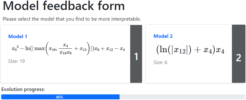
While synthesizing the model, the system shows the user, through a suitable user interface, a query: given a pair of models, the user is asked to tell which one is the most interpretable according to her or his subjective judgment. As soon as the user answers the query (by a single click or tap), ML-PIE shows a new query; internally, it also uses the feedback to update the interpretability estimator. Query-answer interactions continue until the model synthesis process stops because a termination criterion is met. We remark that query-answer interactions and the model synthesis process proceed concurrently and asynchronously (i.e., we do not halt the model synthesis process at any point in time, see Section 7). The interpretability estimator acts as point of contact between the two, as it is updated right after a user’s feedback and is used by the model synthesis process to assess model quality. Figure 2 shows the user interface we used: the user answers the query by simply clicking on the preferred model (in our case, models are formulae).

Design goals

While designing ML-PIE we were driven by two goals. First, we wanted to keep low the annotation effort: we do not ask the users to provide detailed descriptions of what they mean by interpretability, neither do we ask for detailed, informative feedback about the models. Rather, we just ask to compare pairs of models and answer by performing an immediate action (single click or tap). Second, we aimed at obtaining a system that can learn models that are interpretable for a specific user on a specific problem, i.e., we wanted a personalized notion of interpretability. To achieve this goal, we decided to update the interpretability estimator concurrently to the model synthesis process. Note that, this way, the models undergoing user assessment necessarily come from the distribution of models under synthesis. In contrast, performing an off-line annotation approach prior to model synthesis would require to decide a sample of possible models beforehand, some of which may turn out to be unrepresentative of those under synthesis, ultimately wasting part of the user’s effort. Even if ML-PIE updates the estimator while the model synthesis process takes place, we highlight that ML-PIE does not have to start from scratch: a partly pre-trained estimator can be used, as well as one that was previously built for other users, or a similar domain (e.g., healthcare).

Generality and requirements

In principle, our approach is agnostic with respect to the algorithm employed for the model synthesis process and the nature of the models being synthesized, provided that: (a) the former is able to pursue accuracy and interpretability at the same time, either separately with a multi-objective algorithm or jointly with a single-objective one (e.g., to maximize an overall index of trust, we expand on this in Section 7); (b) the latter allows for a visual representation on a user interface (e.g., formulae or decision trees). A further, more practical requirement, is that the speed of the model synthesis process is compatible with allowing the user to provide a sufficient amount of feedback. Our approach is, in principle, also agnostic with respect to the algorithm employed for updating the estimator and the nature of the estimator, provided that these allow for active learning. This last requirement can be met if, e.g., the estimator can produce a measure of uncertainty or confidence when estimating the interpretability of the models (De Freitas et al. 2010).

In this paper, we instantiate ML-PIE for symbolic regression, i.e., our models are symbolic functions expressed as formulae. We use multi-objective GP as model synthesis process. For the estimator, we use a neural network and train it with stochastic gradient descent; to make the network produce predictions with uncertainty, we use dropout at prediction time. In the next section, we describe in detail these key internals of ML-PIE.

4. ML-PIE internals

We choose to use GP in a multi-objective setting because its outcome is a collection of models with different trade-offs between accuracy and interpretability, instead of a single model. This gives the user the possibility to inspect multiple options at the end of the run, and make a final call in terms of overall trustworthiness, i.e., what model meets both acceptable accuracy and interpretability.

Given a supervised learning problem, GP evolves a population of models, here expressed as symbolic functions $f:\mathbb{R}^{d}\to\mathbb{R}$ , such that $f(\boldsymbol{x}_{i})\simeq y_{i},\forall(\boldsymbol{x}_{i},y_{i})$ in the data. The search of GP is driven by two objectives: accuracy, measured on (part of the) data (another being reserved for validation), and interpretability, measured by the interpretability estimator. We describe GP further in Section 4.2. Before that, we describe the neural network used as intepretability estimator (Section 4.1). This estimator takes as input a vector of six features that describe a model $f$ , and produces an output in $\mathbb{R}^{2}$ that represents the interpretability of $f$ and the respective uncertainty.

Following (Virgolin et al. 2020c), the six features of $f$ we use for interpretability estimation are: the total size of $f$ (number of variables plus constants plus operations), the number of operations, the number of operations that are non-arithmetic, the maximum length of consecutive compositions of non-arithmetic operations, the number of constants, and the dimensionality of $f$ (i.e., the number of unique variables)—the latter two being an addition with respect to (Virgolin et al. 2020c).

4.1. The estimator of interpretability

We use a neural network as interpretability estimator because neural networks have excellent fitting capabilities, can produce uncertainty estimations similarly to Gaussian processes by simply making use of dropout at prediction time (Gal and Ghahramani 2016), and their training scales better than that of Gaussian processes (Moore et al. 2016).

The neural network takes the features of a model $f$ as inputs, processes them with three fully-connected hidden layers with $100$ ReLU activations (Nair and Hinton 2010) and $0.25$ dropout rate (Srivastava et al. 2014), and finally applies the hyperbolic tangent. Importantly, we set the network to be trained using binary feedback (i.e., the one provided by the user). Our training signal is constituted by the features of two models $f_{1},f_{2}$ and a label telling which of the two models is more interpretable for the user. Given this training signal, we feed the features of $f_{1}$ and $f_{2}$ as input to the network, and observe how the label compares to the respective predictions of interpretability $\hat{\psi}_{1},\hat{\psi}_{2}$ . Next, we compute a loss that can be seen as a two-points version of the Wasserstein loss commonly used to train generative adversarial networks (Gulrajani et al. 2017):

(1)

\mathcal{L}(\hat{\psi}_{1},\hat{\psi}_{2},l)\vcentcolon=l\left(\hat{\psi}_{1}-\hat{\psi}_{2}\right).

Here, the value of $l$ depends on the label from the user: $l=-1$ if the first model is deemed more interpretable than the second, else $l=1$ . If, e.g., the network predicts that $\hat{\psi}_{1}$ is smaller than $\hat{\psi}_{2}$ but the user prefers $f_{1}$ , then the loss will be positive. We remark that the proposed loss does not provide an explicit signal on what values $\hat{\psi}$ should assume: this is not an issue because for our model synthesis process, i.e., GP, relative values suffice. As optimizer we use stochastic gradient descent ( $\text{learning rate}=0.001,\text{momentum}=0.9$ ).

Active learning with warm-up

As mentioned before, the models that are sent to the user for evaluation are those for which the network has registered the maximal prediction uncertainty so far, i.e., while being used to evaluate the models under synthesis. We measure this uncertainty by applying dropout at prediction time, specifically by taking the standard deviation over repeated predictions $\hat{\psi}^{(1)},\dots,\hat{\psi}^{(k)}$ for a same input model $f$ . We use $k=10$ as a compromise between speed and fidelity, and set the interpretability estimation $\hat{\psi}$ to be the mean of the $k$ predictions.

To avoid relying solely on the feedback of the user, we include an initial warm-up phase using interpretability estimates generated from the estimator of (Virgolin et al. 2020c) for $100$ random models (from now on, we refer to intepretability estimation according to (Virgolin et al. 2020c) by $\phi$ ). We do this because we have no guarantees that the user is responsive, and also so that the initial estimations of interpretability are not completely random. We heuristically halt the warm-up when the uncertainty of the network starts to decrease, specifically when the standard deviations of the predictions of the last two epochs is smaller than that of the previous two on average. Note that an increase of the uncertainty in the initial epochs is a normal consequence of the fact that initialized weights are small (we use Keras default initiliazer (Chollet et al. 2015)), and as they increase with early gradients, so do the magnitudes of the (still semi-random) predictions. We found this scheme to result in around $3$ to $6$ epochs of warm-up.

Justification of adopting a ranking network

Before proceeding, we provide some evidence that the network we adopt, from now on called a ranking network, fares well compared to a more classic network, i.e., one trained as a regressor to predict specific values of interpretability. For the classic network we use the mean squared error loss and use a linear activation to obtain the output (instead of $\tanh$ ). We create a toy scenario where we assume that $\psi:=\phi$ , i.e., we use the estimator from (Virgolin et al. 2020c) in place of the unknown concept of interpretability of the user, and we create labels for a set of $1000$ random symbolic models. Since we use $\phi$ as ground-truth, we change the warm-up phase to use model size ( $\ell$ ) instead of $\phi$ itself, again upon $1000$ random models. For the ranking network, we assume that a feedback consists of a label that tells, given two symbolic models, which is best (as explained before). For the classic network, we have regression labels, i.e., the value of $\phi$ . Note that the number of models-per-feedback is twice for the ranking network than for the classic one. Moreover, providing a label for the classic network requires the user to specify a numeric value, which arguably takes more effort than only telling which of two models is better. For these reasons, we allow the ranking network to receive double the user’s answers than the classic network.

We consider how well the networks are able to induce the same ranking of $\phi$ with increasing amount of feedback, using the Spearman footrule (Spearman 1906; Diaconis and Graham 1977). This measures the misalignment between two rankings $R$ and $S$ (in our case, for $r$ models $f_{1},\dots,f_{r}$ ):

(2)

\textit{Spearman footrule}(R,S)=\frac{3}{q(r)}\sum_{i=1}^{r}|R(f_{i})-S(f_{i})|,

where $q(r)=r^{2}$ is $r$ is even, otherwise $r^{2}-1$ . The term $\frac{3}{q(r)}$ induces a normalization such that the expectation of the footrule is $1$ when the order of one ranking is random with respect to the other, $0$ for identical orders, and $1.5$ for reversed orders. Figure 3 shows results on this toy setting (with respect to a test set of $1000$ random models). On the left panel, it can be seen that the ranking network learns quicker if we ask the user to provide feedback on the models for which the network is most uncertain. On the right panel, it can be seen that the ranking network outperforms the classic network. Note that the initial Spearman footrule is lower than $1$ (value for random ranks) thanks to the warm-up phase on $\ell$ .

Figure 3. Capability of neural networks to learn the same ordering induced by

\phi

as a function of the amount of feedback (median

=

solid, mean

=

dashed, interquartile range

=

shaded area, across

30

repetitions). A warm-up phase is applied using

\ell

. Left: Prioritizing uncertainty to decide what models to submit for feedback improves the learning speed of the ranking network. Right: The ranking network adapts more quickly than the classic network.

4.2. Bi-objective evolution

We use the GP version of the well-known NSGA-II algorithm (Deb et al. 2000) implemented in (Virgolin et al. 2020c)¹¹ 1 Code available at: https://github.com/marcovirgolin/pyNSGP. The models evolved by GP, i.e., the symbolic functions, are represented with a traditional tree-based encoding (Poli et al. 2008). At initialization, the trees are generated using the ramped half-and-half method, with tree depth between $1$ and $3$ . The trees are rather small, and are allowed to have at most up to $25$ components (nodes) at any point during the evolution, because larger trees quickly becomes incomprehensible. Trees that are selected with tournaments of size $2$ undergo modification by means of traditional subtree crossover, subtree mutation, and one-point mutation, with equal probability.

Our GP uses two objectives. The first objective is maximizing accuracy (for regression, we actually minimize the mean squared error). We include linear scaling (Keijzer 2004) to adapt the fitting of the evolving models, since it is often beneficial on real-world datasets (Virgolin et al. 2019). The second objective is maximizing interpretability. In ML-PIE, this is estimated ( $\hat{\psi}$ ) by our interpretability estimator. For comparison, we also consider using $\phi$ (estimation according to (Virgolin et al. 2020c)) and $\ell$ (the model size, i.e., number of tree nodes). The outcome of GP is a collection of models that expresses a trade-off front of the objectives, i.e., taken any two models “from the front”, if the first has better accuracy, then it must have worse interpretability (and vice versa).

The primitives used to evolve symbolic functions are (a) the variables of the problem at hand; (b) random constants between $-5$ and $5$ with resolution of $0.25$ ; (c) the functions $+$ , $-$ , $\times$ , $\div^{*}$ , $\cdot^{3}$ , $\log^{*}$ , $\max$ (^∗=protected). We use a relatively small population of $256$ models and evolve it for $50$ generations. We found this to be a good compromise between what performance the models can achieve, and how much time the users need to spend to terminate a run of ML-PIE (i.e., approx. $10$ minutes). Since the population is not large, we include a simple method to oppose premature convergence that worked remarkably well in preliminary experiments. Specifically, for each model $f_{p}$ in the population (parsed in a random order), we check whether another model $f_{q}$ co-exists that has the same behavior (with respect to the data, i.e., $\forall\boldsymbol{x}_{i},f_{p}(\boldsymbol{x}_{i})=f_{q}(\boldsymbol{x}_{i})$ ); for any such $f_{q}$ , we mark it as duplicate (note, we do not mark the first $f_{p}$ ). Models marked as duplicates are set to have the lowest priority when GP selects parents and chooses the survivors of the generation.

5. Experimental Setup

We asked students enrolled at the engineering faculties of the University of Trieste, Italy and Chalmers University of Technology, Sweden to act as users for ML-PIE, which we disseminated as a web application on the cloud. Data collection lasted for approximately two weeks.

Experiments were run on two datasets, namely Boston housing (in short, Boston) and German credit (German), which concern regression of housing values and binary classification of credit approval, respectively. These datasets from the UCI repository (Dua and Graff 2017) are well-known, of moderate-enough size to keep the users busy only for a reasonable time, and also interesting for assessing fairness in AI, because Boston includes a feature regarding race, while German has one regarding sex. Boston has $506$ examples and $13$ features, while German has $1000$ examples and $20$ features. With the parameter settings used for GP, it takes approximately $10$ minutes to complete a run of ML-PIE; the estimation of interpretability by the neural network taking most computation time. Each run used a random split of the dataset in exam, namely into $70\text{\,}\mathrm{\%}$ of the examples for training and $30\text{\,}\mathrm{\%}$ for testing. The features of the datasets were standardized by z-scoring (Dick et al. 2020).

We also prepared an experiment to assess whether ML-PIE is any better than using pre-existing indices of interpretability, namely $\phi$ and $\ell$ . To this end, at the end of each ML-PIE run, the users were presented with a set of models from the trade-off front obtained during the run (i.e., by GP using $\hat{\psi}$ ) paired with models taken from runs where GP used $\phi$ or $\ell$ as indices of interpretability ( $100$ pre-computed runs for each). Models in each pair ( $\hat{\psi}$ vs. $\phi$ or $\hat{\psi}$ vs. $\ell$ ) had similar accuracy (pairing made by considering the minimal absolute difference). The users were asked to tell, for each pair, which of the two models was more interpretable. The users were not told which models were found during their session (i.e., with $\hat{\psi}$ ) and which were found using $\phi$ or $\ell$ , to prevent bias.

6. Results

We show key results regarding the workings of ML-PIE and the performance it achieves. A total of $61$ users answered the call, leading to $49$ runs for Boston and $45$ runs on German (some students did not run both). In the following, we report: how the users and the estimator of interpretability behaved during the runs (Section 6.1); the search performance of ML-PIE compared to that obtainable when $\phi$ or $\ell$ are used (Section 6.2); whether estimations of interpretability $\hat{\psi}$ obtained by different users behave differently (Section 6.3); and, last but not least, whether the users preferred models discovered using $\hat{\psi}$ over models found by $\phi$ or $\ell$ (Section 6.4).

6.1. Behavior of the users and of the interpretability estimator

Figure 4 summarizes how the users and the estimator behaved over time. In the top panel, we see that the amount of feedback given per generation tends to be slightly smaller for early generations. We remark that this is because, in GP, the average model size tends to grow over time, causing early generations to be computed more quickly than later ones, and the users to have less time to provide feedback. We also measured the rate at which the estimator made mispredictions, by checking whether the estimates $\hat{\psi}_{1},\hat{\psi}_{2}$ for the respective models $f_{1}$ and $f_{2}$ before the user’s answer turned out to be in disagreement with the user’s answer (e.g., $\hat{\psi}_{1}<\hat{\psi}_{2}$ but the user picks $f_{1}$ ). Mispredictions were quite rare. This result is in line with what can be seen on the bottom panel, i.e., that the uncertainty of the estimator (the standard deviation of its estimations $\sigma(\hat{\psi})$ ) dropped rather quickly and remained low over time. We also see that the cumulative amount of feedback had a steady, linear growth.

Table 1 shows examples of models²² 2 We do not perform model simplification because too costly to perform upon each model being evolved, it might harm evolvability, and, if done only for the models displayed to the user, it may create a perception mismatch with respect to the features of the models (size, no. operators, etc.), used by the interpretability estimator. extracted from the trade-off fronts obtained by the user-guided evolutions, at different trade-off levels between accuracy and interpretability (interpretability percentile $\tau$ ). Note that we actually report errors: the training and test errors for Boston are mean squared errors, while those for German are inaccuracies ( $1-\text{accuracy}$ ). It can clearly be seen that, the more we move from more accurate models to more interpretable ones (i.e., increasing $\tau$ ), the more the models become simpler under several aspects, such as total size, number of dimensions, and presence of non-arithmetic operations. This confirms that the estimator was capable of capturing a sensible notion of interpretability. A further confirmation of this is provided later in Section 6.3.

Take-home. Overall, the users provided good amounts of feedback through the process, and the estimator of interpretetability responded in a sensible manner. Observed uncertanties, mispredictions, and model ranking behaviors, are reasonable.

Table 1. Examples of models discovered by evolutions guided by the users. The models are taken at random from the evolved trade-off fronts (training error vs.

\hat{\psi}

) at different interpretability percentiles (

\tau

). The test error is also reported, and some amount of overfitting can be observed (most notably, the first model at

\tau=10

for Boston). Our approach is capable of capturing sensible trends of model intepretability: models become simpler as

\tau

increases.

Dataset	$\tau$	Train	Test	Model
Boston	10	$18.43$	$37.53$	$x_{12}-\operatorname{max}\left(2.5,x_{8}+x_{9}+x_{5}-x_{8}-x_{2}\right)\left(-0.25+x_{12}\right)+\operatorname{max}\left(x_{5},x_{12}\right)$
		$19.86$	$18.57$	$4.5\times x_{12}+x_{5}\left(x_{10}+\frac{x_{9}}{x_{5}}\right)+\left(x_{12}+x_{10}\right)x_{5}+x_{12}+x_{5}\left(-3.25-x_{5}\right)$
		$21.24$	$20.07$	$\operatorname{max}\left(x_{11}x_{11}x_{11},\ln(\left\|x_{5}\left(x_{5}-x_{12}\right)\right\|)\right)-x_{12}+x_{5}-\operatorname{max}\left(x_{0},2.5\right)+x_{12}+x_{10}$
	50	$25.64$	$30.16$	$x_{12}-\operatorname{max}\left(x_{12},x_{5}\right)$
		$26.05$	$35.42$	$\frac{-1.0+x_{4}}{4.25}-4.75-1.75-\left(x_{12}+x_{10}-x_{5}\right)\times 4.75$
		$32.13$	$29.09$	$\frac{x_{12}}{x_{12}}\left(x_{12}+x_{12}-x_{5}\right)$
	90	$35.47$	$45.54$	$\frac{x_{12}}{-2.75}\times-0.25$
		$57.82$	$61.84$	$x_{10}-x_{11}$
		$71.97$	$62.50$	$3.0-x_{4}$
German	10	$0.24$	$0.26$	$x_{1}-x_{0}-x_{6}+x_{7}+x_{11}-x_{6}+\frac{x_{1}}{x_{17}}-x_{2}-x_{0}$
		$0.25$	$0.24$	$x_{4}+x_{19}-x_{10}+\frac{x_{0}}{x_{16}}-x_{1}+x_{18}-x_{1}-x_{1}+x_{5}-x_{6}-x_{6}$
		$0.25$	$0.25$	$x_{2}+x_{2}+x_{8}+x_{0}-x_{1}$
	50	$0.25$	$0.24$	$\left(x_{2}-x_{4}x_{4}+x_{1}-x_{4}-4.5\right)x_{0}$
		$0.25$	$0.27$	$x_{11}-2.5-x_{2}-x_{0}+3.25$
		$0.26$	$0.30$	$x_{4}-x_{0}-x_{0}$
	90	$0.26$	$0.29$	$x_{11}-x_{0}$
		$0.26$	$0.30$	$x_{0}-x_{4}+x_{5}$
		$0.28$	$0.26$	$x_{2}+x_{0}$

Figure 4. User and framework behavior over the number of generations (median

=

solid, mean

=

dashed, interquartile range

=

shaded area, across all users). Top: Amount of feedbacks given and percentage of mispredictions made by the intepretability estimator, per generation. Bottom: Cumulative amount of feedback and estimator uncertainty

\sigma(\hat{\psi})

over the generations. Uncertainty is normalized by dividing by the average uncertainty observed at the first generation.

6.2. Search performance

Table 2 summarizes the search performance of GP using $\hat{\psi}$ (over the runs performed during the feedback sessions with the users, $49$ for Boston and $45$ for German), $\phi$ , and $\ell$ ( $100$ runs per dataset for each). Before delving into $\hat{\psi}$ , we remark that the results obtained by $\phi$ and $\ell$ are similar to those reported in literature (see, e.g., (Virgolin et al. 2020c) for Boston³³ 3 Besides front sizes, this can be checked by de-normalizing the errors reported in Table 2 of (Virgolin et al. 2020c) by multiplying them with the variance of the label, i.e., $\approx 84.6$ . and (Mota et al. 2021; Setzu et al. 2021) for German), despite the fact that our GP used limited resources ( $\text{population size}=256,\text{generations}=50$ ).

What can be mainly drawn from Table 2 is that, error-wise, results with $\hat{\psi}$ can be slightly worse than those obtained with $\phi$ and $\ell$ . However, this is rarely important (e.g., only statistically significant in two cases at test time, for $\tau=50$ ). Likely, this is a consequence of the fact that the estimator of $\hat{\psi}$ is stochastic (due to dropout) and is only refined over time. Noisy objectives are known to hinder search algorithms, including evolutionary ones (Beyer 2000; Rakshit et al. 2017). This fact also justifies larger front sizes being produced by $\hat{\psi}$ . We note that if we restrict the results with $\hat{\psi}$ to only account for good amounts of feedback being given, e.g., $\geq 100$ (approximately $50\text{\,}\mathrm{\%}$ ), results do not change substantially.

Take-home. Model accuracy is slightly worse when $\hat{\psi}$ is used instead of $\phi$ or $\ell$ . This is likely because the estimator is noisy. A simple action that can be taken is to increase GP search resources.

Dataset		Boston				German
$\tau$		0	10	30	50	0	10	30	50
$\hat{\psi}$	Front	12.4				10.9
	Train	$20.06$	$21.06$	$23.32$	$27.78$	$0.23$	$0.24$	$0.25$	$0.26$
	Test	$22.43$	$23.19$	$24.65$	$28.93$	$0.26$	$0.26$	$0.27$	$0.27$
$\phi$	Front	9.3				5.4
	Train	$19.09$	19.39	20.94	23.24	$0.24$	$0.24$	$0.24$	$0.25$
	Test	$22.62$	$21.92$	$22.44$	24.98	$0.27$	$0.27$	$0.27$	$0.28$
$\ell$	Front	9.1				6.9
	Train	$18.70$	19.03	20.54	22.35	$0.24$	$0.24$	$0.24$	$0.25$
	Test	$22.39$	$22.68$	$23.08$	24.24	$0.27$	$0.27$	$0.27$	$0.28$

Table 2. Mean front sizes (Front), and mean train and test errors (respectively Train and Test), at different interpretability percentiles (

\tau

) of the models in the best-found trade-off fronts, for GP using

\hat{\psi}

\phi

, or

\ell

as interpretablity indices. Errors in bold are significantly better than their

\hat{\psi}

counterpart (Mann-Whitney U test

p\text{-value}<0.01

with Bonferroni correction).

6.3. Level of personalization

Figure 5 shows comparisons of rankings induced by different users with respect to each other and with respect to $\phi$ and $\ell$ . We now use the notation $\hat{\psi}_{i}$ to refer to the interpretability estimates for a certain $i$ -th user. The rankings are computed by ordering, according to $\phi$ , $\ell$ , and each $\hat{\psi}_{i}$ , all models from the fronts ever discovered by all the users (excluding syntactic duplicates and totalling $\approx$9000$$ models).

We begin by observing that the distributions of Spearman footrule obtained when comparing user induced-rankings with one another ( $\hat{\psi}_{i}$ vs. $\hat{\psi}_{j}$ ) can have heavy or long tails. Overall, this corroborates the hypothesis that some users may have non-negligible disagreements regarding their notions of interpretability, and thus that seeking personalized interpretability estimations is needed.

Average behaviors are also interesting. On average, user induced-rankings are more similar to one another (footrule of $\hat{\psi}_{i}$ vs. $\hat{\psi}_{j}$ has average value of $\approx 0.13$ ) than to those induced by $\phi$ or $\ell$ (respectively $\hat{\psi}_{i}$ vs. $\phi$ with average value $\approx 0.2$ and $\hat{\psi}_{i}$ vs. $\ell$ with average value $\approx 0.25$ ). This means that, on average, users provided similar feedback, i.e., they agreed on a similar notion of interpretability $\psi$ (at least, for the experimental setting we proposed and for the users involved). Furthermore, note that user induced-rankings are more similar to those of $\phi$ and $\ell$ than how the ranking of $\phi$ is similar to that of $\ell$ . This means that the average $\hat{\psi}_{i}$ has more in common with $\phi$ and $\ell$ than the latter two have with each other.

Take-home. The estimations can be personalized (long tails of $\hat{\psi}_{i}$ vs. $\hat{\psi}_{j}$ ) but are similar on average (footrule of $\approx 0.13$ ), conditioned to our experimental settings and involved cohort (students).

Figure 5. Violin plot of Spearman footrules from comparing rankings obtained with different interpretability estimators. On average, a user’s estimated interpretability

\hat{\psi}_{i}

is more similar to that of another user

\hat{\psi}_{j}

than to

\phi

and

\ell

. However, high disagreements are also possible (fat and long tail for Boston, very long tail for German).

6.4. Final user judgment on $\hat{\psi}$ , $\phi$ , and $\ell$

Figure 6 shows the preferences indicated by the users when presented, at the end of an ML-PIE run, with models found by the run itself at $\tau=30$ and $\tau=50$ , and similarly accurate models obtained in pre-performed runs using $\phi$ and $\ell$ .

The first result we highlight is that, for sufficiently simple models (i.e., $\tau=50$ , cfr. Table 1), it does not seem to matter what interpretability index is used. Conversely, preferences start to emerge when more complex models are at play, i.e., at $\tau=30$ . In $\hat{\psi}$ vs. $\phi$ comparisons (top panels), we see that models discovered by our approach were preferred over those found using $\phi$ almost $15\text{\,}\mathrm{\%}$ of the times for Boston, and $10\text{\,}\mathrm{\%}$ of the times for German. The biggest difference at $\tau=30$ happens for $\hat{\psi}$ vs. $\ell$ for Boston (bottom left panel), with a $20\text{\,}\mathrm{\%}$ preference gain for $\hat{\psi}$ . For German at $\tau=30$ , however, $\ell$ was preferred over $\hat{\psi}$ by approximately $7\text{\,}\mathrm{\%}$ . We can justify this result by looking back at Table 1, where it can be sees that the more complex models found for German ( $\tau=10$ ) are actually not that complex after all (e.g., they all lack non-arithmetic operations). On this dataset, decent accuracy can already be obtained when the models are linear, hence minimizing size seems to be sufficient. Note that, by contrast, the models found for Boston can be much more complex.

Take-home. Overall, for more complex models, the users indicated a preference for the models found with ML-PIE over those found using $\phi$ or $\ell$ . However, for simpler models, $\ell$ suffices.

Figure 6. Outcome of the survey at the end of the evolution. For

\tau=50

, it largely does not matter what index of interpretability is used. When the models start to be more complex, i.e., for

\tau=30

, the users generally prefer

\hat{\psi}

over

\phi

and

\ell

, except for

\hat{\psi}

vs.

\ell

on German.

7. Discussion & conclusion

We believe that our results, obtained on two datasets and involving $61$ engineering students, are promising. The results show that ML-PIE behaves sensibly, the search performance of GP is not harmed excessively by $\hat{\psi}$ being noisy, different users can induce different $\hat{\psi}$ , and the models obtained by ML-PIE tend to be preferred over those obtained when $\phi$ or $\ell$ are used instead.

Regarding the last point, preference for $\hat{\psi}$ over $\phi$ and $\ell$ is, however, only marginal. We believe that this result is a consequence of what can be considered the main limitation of this study: we did not involve actual domain experts and used a rather general set of model features to estimate model interpretability. Since our users (engineering students) were not experts in housing values (for Boston) nor credit approval risk (for German), we did not provide them with the meaning of the features of the datasets, nor we asked them to attempt to understand what the models in exam exactly mean. Yet, relying on students allowed us to have a decently-sized cohort with some general knowledge about formulae: we believe that this allowed us to gain sufficient evidence that ML-PIE works sensibly. We think that even if the preference gains obtained by $\hat{\psi}$ over $\phi$ and $\ell$ were moderate, they represent a very promising result: by enabling the interpretability estimator to use more specialized model features (e.g., what domain-specific features and functions appear, how many times, and in which context), and involving actual domain experts, it is reasonable to expect that the preference for $\hat{\psi}$ will increase substantially.

From a technical standpoint, there are a number of aspects worth studying to improve ML-PIE. For example, while we used a neural network with sensible settings to realize the interpretability estimator, we did not, e.g., optimize its architecture. Another point that deserves further investigation is concurrency aspects. We designed ML-PIE to make the user provide feedback while the model synthesis process is ongoing because, this way, the models that require user assessment come directly from the distribution of models under synthesis—and not from a potentially-unrepresentative sample, wasting (part of) the user’s effort. However, the pace of feedback provided by the user may be too slow with respect to the speed of the model synthesis process, ultimately harming it. It may be beneficial to study whether the model synthesis process should be halted at times, e.g., based on statistics regarding the uncertainty of the interpretability estimator.

In the future, together with involving domain experts and adding representative power to the estimator of interpretability (e.g., enabling more model features to be accounted for), we plan to demonstrate that ML-PIE can be adapted to other settings than formulae-like models (e.g., decision trees) and other model synthesis processes than evolutionary ones (e.g., single-objective reinforcement learning or multi-objective gradient descent (Deist et al. 2021)). Regarding the last point, it would be interesting to study whether model synthesis can be guided exclusively by user feedback, to optimize some overall measure of trust (Ferrario et al. 2019), e.g., a measure that encapsulates, at once, accuracy, interpretability, and possibly other aspects such as soundness (e.g., for models that must satisfy physical constraints).

Concluding, we propose Model Learning with Personalized Interpretability Estimation (ML-PIE), a human-in-the-loop, active learning approach for the synthesis of models with user-tailored interpretability. ML-PIE answers the need for eXplainable AI (XAI) methods capable of synthesizing models that have a chance of being interpretable at a personalized level. Our experiments involving $61$ students of engineering show that ML-PIE is capable of learning, from their feedback, user-specific estimations of interpretability. These estimations can be substantially different for different users, and are in general different from interpretability indices from literature. Last but not least, the users show a moderate preference for the models synthesized using their own feedback over models synthesized when other interpretability indices are used.

We believe that this work shows that XAI methods capable of model synthesis with personalized interpretability can be achieved. These methods may bring profound advantages for the responsible use of AI in high-stakes societal applications.

References

(1)
Adadi and Berrada (2018) Amina Adadi and Mohammed Berrada. 2018. Peeking inside the black-box: A survey on eXplainable Artificial Intelligence (XAI). IEEE Access 6 (2018), 52138–52160.
Bartoli et al. (2017) Alberto Bartoli, Andrea De Lorenzo, Eric Medvet, and Fabiano Tarlao. 2017. Active learning of regular expressions for entity extraction. IEEE Transactions on Cybernetics 48, 3 (2017), 1067–1080.
Benk and Ferrario (2020) Michaela Benk and Andrea Ferrario. 2020. Explaining Interpretable Machine Learning: Theory, Methods and Applications. SSRN Methods and Applications.
Beyer (2000) Hans-Georg Beyer. 2000. Evolutionary algorithms in noisy environments: Theoretical issues and guidelines for practice. Computer Methods in Applied Mechanics and Engineering 186, 2-4 (2000), 239–267.
Breslow and Aha (1997) Leonard A. Breslow and David W. Aha. 1997. Simplifying decision trees: A survey. Knowledge engineering review 12, 1 (1997), 1–40.
Cano et al. (2013) Alberto Cano, Amelia Zafra, and Sebastián Ventura. 2013. An interpretable classification rule mining algorithm. Information Sciences 240 (2013), 1–20.
Chollet et al. (2015) François Chollet et al. 2015. Keras. https://keras.io.
Christiano et al. (2017) Paul F. Christiano, Jan Leike, Tom B. Brown, Miljan Martic, Shane Legg, and Dario Amodei. 2017. Deep reinforcement learning from human preferences. In Proceedings of the 31st International Conference on Neural Information Processing Systems. Curran Associates, Inc., 4302–4310.
Custode and Iacca (2020) Leonardo L. Custode and Giovanni Iacca. 2020. Evolutionary learning of interpretable decision trees. arXiv preprint arXiv:2012.07723 (2020).
De Freitas et al. (2010) Junio De Freitas, Gisele L. Pappa, Altigran S. da Silva, Marcos A. Gonc, Edleno Moura, Adriano Veloso, Alberto H.F. Laender, and Moisés G. de Carvalho. 2010. Active learning genetic programming for record deduplication. In IEEE Congress on Evolutionary Computation. IEEE, IEEE, 1–8.
Deb et al. (2000) Kalyanmoy Deb, Samir Agrawal, Amrit Pratap, and Tanaka Meyarivan. 2000. A fast elitist non-dominated sorting genetic algorithm for multi-objective optimization: NSGA-II. In International Conference on Parallel Problem Solving from Nature. Springer Berlin Heidelberg, 849–858.
Deist et al. (2021) Timo M. Deist, Monika Grewal, Frank J. W. M. Dankers, Tanja Alderliesten, and Peter A. N. Bosman. 2021. Multi-Objective Learning to Predict Pareto Fronts Using Hypervolume Maximization. arXiv preprint arXiv:2102.04523 (2021).
Diaconis and Graham (1977) Persi Diaconis and Ronald L. Graham. 1977. Spearman’s footrule as a measure of disarray. Journal of the Royal Statistical Society: Series B (Methodological) 39, 2 (1977), 262–268.
Dick et al. (2020) Grant Dick, Caitlin A. Owen, and Peter A. Whigham. 2020. Feature Standardisation and Coefficient Optimisation for Effective Symbolic Regression. In Proceedings of the Genetic and Evolutionary Computation Conference. Association for Computing Machinery, 306–314.
Dua and Graff (2017) Dheeru Dua and Casey Graff. 2017. UCI Machine Learning Repository. http://archive.ics.uci.edu/ml
Ekárt and Nemeth (2001) Anikó Ekárt and Sandor Z. Nemeth. 2001. Selection based on the Pareto nondomination criterion for controlling code growth in genetic programming. Genetic Programming and Evolvable Machines 2, 1 (2001), 61–73.
Ferrario et al. (2019) Andrea Ferrario, Michele Loi, and Eleonora Viganò. 2019. In AI we trust Incrementally: A Multi-layer model of trust to analyze Human-Artificial intelligence interactions. Philosophy & Technology 33 (2019), 1–17.
Freitas (2014) Alex A. Freitas. 2014. Comprehensible classification models: A position paper. ACM SIGKDD Explorations Newsletter 15, 1 (2014), 1–10.
Gal and Ghahramani (2016) Yarin Gal and Zoubin Ghahramani. 2016. Dropout as a Bayesian approximation: Representing model uncertainty in deep learning. In International Conference on Machine Learning. JMLR.org, 1050–1059.
Guidotti et al. (2018) Riccardo Guidotti, Anna Monreale, Salvatore Ruggieri, Franco Turini, Fosca Giannotti, and Dino Pedreschi. 2018. A survey of methods for explaining black box models. ACM Computing Surveys (CSUR) 51, 5 (2018), 1–42.
Gulrajani et al. (2017) Ishaan Gulrajani, Faruk Ahmed, Martin Arjovsky, Vincent Dumoulin, and Aaron Courville. 2017. Improved training of Wasserstein GANs. In Proceedings of the 31st International Conference on Neural Information Processing Systems (Long Beach, California, USA) (NIPS’17). Curran Associates Inc., 5769–5779.
Hatherley (2020) Joshua James Hatherley. 2020. Limits of trust in medical AI. Journal of Medical Ethics 46, 7 (2020), 478–481.
Hein et al. (2018) Daniel Hein, Steffen Udluft, and Thomas A. Runkler. 2018. Interpretable policies for reinforcement learning by genetic programming. Engineering Applications of Artificial Intelligence 76 (2018), 158–169.
Huysmans et al. (2011) Johan Huysmans, Karel Dejaeger, Christophe Mues, Jan Vanthienen, and Bart Baesens. 2011. An empirical evaluation of the comprehensibility of decision table, tree and rule based predictive models. Decision Support Systems 51, 1 (2011), 141–154.
Isele and Bizer (2013) Robert Isele and Christian Bizer. 2013. Active learning of expressive linkage rules using genetic programming. Journal of Web Semantics 23 (2013), 2–15.
Izza et al. (2020) Yacine Izza, Alexey Ignatiev, and Joao Marques-Silva. 2020. On explaining decision trees. arXiv preprint arXiv:2010.11034 (2020).
Jobin et al. (2019) Anna Jobin, Marcello Ienca, and Effy Vayena. 2019. The global landscape of AI ethics guidelines. Nature Machine Intelligence 1, 9 (2019), 389–399.
Keijzer (2004) Maarten Keijzer. 2004. Scaled symbolic regression. Genetic Programming and Evolvable Machines 5, 3 (2004), 259–269.
Koza (1992) John R. Koza. 1992. Genetic programming: On the programming of computers by means of natural selection. Vol. 1. MIT Press.
Lakkaraju et al. (2016) Himabindu Lakkaraju, Stephen H. Bach, and Jure Leskovec. 2016. Interpretable decision sets: A joint framework for description and prediction. In Proceedings of the 22nd ACM SIGKDD International Conference on Knowledge Discovery and Data Mining. Association for Computing Machinery, 1675–1684.
Lensen (2021) Andrew Lensen. 2021. Mining Feature Relationships in Data. In Genetic Programming: 24th European Conference, EuroGP 2021, Held as Part of EvoStar 2021, Vol. 12691. Springer, Cham, 247–262.
Lensen et al. (2020) Andrew Lensen, Bing Xue, and Mengjie Zhang. 2020. Genetic programming for evolving a front of interpretable models for data visualization. IEEE Transactions on Cybernetics (2020), 1–15.
Letham et al. (2015) Benjamin Letham, Cynthia Rudin, Tyler H. McCormick, and David Madigan. 2015. Interpretable classifiers using rules and Bayesian analysis: Building a better stroke prediction model. Annals of Applied Statistics 9, 3 (2015), 1350–1371.
Lipton (2018) Zachary C. Lipton. 2018. The Mythos of Model Interpretability: In machine learning, the concept of interpretability is both important and slippery. Queue 16, 3 (2018), 31–57.
Mahoor et al. (2017) Zahra Mahoor, Jack Felag, and Josh Bongard. 2017. Morphology dictates a robot’s ability to ground crowd-proposed language. arXiv preprint arXiv:1712.05881 (2017).
Medvet et al. (2015) Eric Medvet, Alberto Bartoli, Barbara Carminati, and Elena Ferrari. 2015. Evolutionary inference of attribute-based access control policies. In International Conference on Evolutionary Multi-Criterion Optimization. Springer, Cham, 351–365.
Molnar (2020) Christoph Molnar. 2020. Interpretable machine learning — A guide for making black box models explainable. Lulu.com.
Molnar et al. (2020) Christoph Molnar, Gunnar König, Julia Herbinger, Timo Freiesleben, Susanne Dandl, Christian A. Scholbeck, Giuseppe Casalicchio, Moritz Grosse-Wentrup, and Bernd Bischl. 2020. Pitfalls to avoid when interpreting machine learning models. arXiv preprint arXiv:2007.04131 (2020).
Moore et al. (2016) Christopher J. Moore, Alvin J. K. Chua, Christopher P. L. Berry, and Jonathan R. Gair. 2016. Fast methods for training Gaussian processes on large datasets. Royal Society Open Science 3, 5 (2016), 160125.
Mota et al. (2021) Douglas Mota, Enrique Naredo, and Conor Ryan. 2021. Towards Incorporating Human Knowledge in Fuzzy Pattern Tree Evolution. In Genetic Programming: 24th European Conference, EuroGP 2021, Held as Part of EvoStar 2021. Springer International Publishing, 66–81.
Nair and Hinton (2010) Vinod Nair and Geoffrey E. Hinton. 2010. Rectified linear units improve restricted Boltzmann machines. In International Conference on Machine Learning. Omnipress, 807–814.
Poli et al. (2008) Riccardo Poli, William B Langdon, Nicholas F McPhee, and John R Koza. 2008. A field guide to genetic programming. Lulu.com.
Poursabzi-Sangdeh et al. (2018) Forough Poursabzi-Sangdeh, Daniel G. Goldstein, Jake M. Hofman, Jennifer Wortman Vaughan, and Hanna Wallach. 2018. Manipulating and measuring model interpretability. arXiv preprint arXiv:1802.07810 (2018).
Rakshit et al. (2017) Pratyusha Rakshit, Amit Konar, and Swagatam Das. 2017. Noisy evolutionary optimization algorithms–A comprehensive survey. Swarm and Evolutionary Computation 33 (2017), 18–45.
Rudin (2019) Cynthia Rudin. 2019. Stop explaining black box machine learning models for high stakes decisions and use interpretable models instead. Nature Machine Intelligence 1, 5 (2019), 206–215.
Secretan et al. (2011) Jimmy Secretan, Nicholas Beato, David B. D’Ambrosio, Adelein Rodriguez, Adam Campbell, Jeremiah T. Folsom-Kovarik, and Kenneth O. Stanley. 2011. Picbreeder: A case study in collaborative evolutionary exploration of design space. Evolutionary Computation 19, 3 (2011), 373–403.
Settles (2009) Burr Settles. 2009. Active learning literature survey. Technical Report. University of Wisconsin-Madison Department of Computer Sciences.
Setzu et al. (2021) Mattia Setzu, Riccardo Guidotti, Anna Monreale, Franco Turini, Dino Pedreschi, and Fosca Giannotti. 2021. GLocalX—From Local to Global Explanations of Black Box AI Models. Artificial Intelligence 294 (2021), 103457.
Smits and Kotanchek (2005) Guido F. Smits and Mark Kotanchek. 2005. Pareto-front exploitation in symbolic regression. In Genetic Programming Theory and Practice II. Springer, 283–299.
Spearman (1906) Charles Spearman. 1906. Footrule for measuring correlation. British Journal of Psychology 2, 1 (1906), 89.
Srivastava et al. (2014) Nitish Srivastava, Geoffrey Hinton, Alex Krizhevsky, Ilya Sutskever, and Ruslan Salakhutdinov. 2014. Dropout: A Simple Way to Prevent Neural Networks from Overfitting. Journal of Machine Learning Research 15, 1 (2014), 1929–1958.
Su et al. (2015) Guolong Su, Dennis Wei, Kush R. Varshney, and Dmitry M. Malioutov. 2015. Interpretable two-level boolean rule learning for classification. arXiv preprint arXiv:1511.07361 (2015).
Tibshirani (1996) Robert Tibshirani. 1996. Regression shrinkage and selection via the LASSO. Journal of the Royal Statistical Society: Series B (Methodological) 58, 1 (1996), 267–288.
Ustun and Rudin (2016) Berk Ustun and Cynthia Rudin. 2016. Supersparse linear integer models for optimized medical scoring systems. Machine Learning 102, 3 (2016), 349–391.
Virgolin et al. (2019) Marco Virgolin, Tanja Alderliesten, and Peter A. N. Bosman. 2019. Linear scaling with and within semantic backpropagation-based genetic programming for symbolic regression. In Proceedings of the Genetic and Evolutionary Computation Conference. Association for Computing Machinery, 1084–1092.
Virgolin et al. (2020a) Marco Virgolin, Tanja Alderliesten, and Peter A. N. Bosman. 2020a. On explaining machine learning models by evolving crucial and compact features. Swarm and Evolutionary Computation 53 (2020), 100640.
Virgolin et al. (2020b) Marco Virgolin, Tanja Alderliesten, Cees Witteveen, and Peter A. N. Bosman. 2020b. Improving model-based genetic programming for symbolic regression of small expressions. Evolutionary computation (2020), tba.
Virgolin et al. (2020c) Marco Virgolin, Andrea De Lorenzo, Eric Medvet, and Francesca Randone. 2020c. Learning a formula of interpretability to learn interpretable formulas. In International Conference on Parallel Problem Solving from Nature. Springer, Cham, 79–93.
Vladislavleva et al. (2008) Ekaterina J. Vladislavleva, Guido F. Smits, and Dick Den Hertog. 2008. Order of nonlinearity as a complexity measure for models generated by symbolic regression via Pareto genetic programming. IEEE Transactions on Evolutionary Computation 13, 2 (2008), 333–349.
Wang and Rudin (2015) Fulton Wang and Cynthia Rudin. 2015. Falling rule lists. In Artificial Intelligence and Statistics. PMLR, 1013–1022.
Wang et al. (2017) Tong Wang, Cynthia Rudin, Finale Doshi-Velez, Yimin Liu, Erica Klampfl, and Perry MacNeille. 2017. A Bayesian framework for learning rule sets for interpretable classification. The Journal of Machine Learning Research 18, 1 (2017), 2357–2393.
Yang and Loog (2016) Yazhou Yang and Marco Loog. 2016. Active learning using uncertainty information. In 23rd International Conference on Pattern Recognition (ICPR). IEEE, 2646–2651.
Zou and Hastie (2005) Hui Zou and Trevor Hastie. 2005. Regularization and variable selection via the elastic net. Journal of the Royal Statistical Society: Series B (Methodological) 67, 2 (2005), 301–320.