Communication Efficient Federated Learning with Adaptive QuantizationDOI: 10.1145/1122445.1122456Journal: JACMVolume: 3741118CCS: Computing methodologies Artificial intelligenceCCS: Computing methodologies Machine learningCCS: Networks Network reliability

FL is designed to collaboratively train a global machine learning model with heterogeneous local data distribution across multiple privacy-sensitive clients. A typical architecture for a FL system with $M$ distributed clients and a server is shown in Fig. 1. Similar to most distributed learning systems, FL system uses a server to receive locally-computed gradients and update global model by aggregation. However, in order to prevent privacy leakage from raw gradients, distributed clients have to mask or encrypt the local gradients before transmission. Therefore, the communication burden in FL systems tends to be heavier compared with other distributed learning systems(Bonawitz et al. 2017). Besides, distributed clients in FL systems, such as mobile devices in wireless networks, usually have limited computation and communication resources, which may lead to the dropout of the participants in each iteration, like the client $M$ shown in Fig. 1. Thus, the robustness to client dropout is another practical requirement for FL systems(Bonawitz et al. 2017).

FL is bottlenecked by the high communication overheads and limited device reliability. The lack of efficient transmission and robustness to client dropouts may lead to slow, expensive and unstable learning. In this paper, the FL framework with the proposed AQG method provides opportunities for communication-efficient FL with large-scale of client dropouts.

Firstly, AQG focuses on reducing unnecessary transmission by fully utilizing the heterogeneous property of FL. Due to the heterogeneousness of local data distribution, local optimization objectives descend at different rates. Therefore, adaptively adjusting the quantization level according to gradient’s update amount provides a more efficient way to communicate with the server by quantizing slowly-varying gradients with less amount of bits.

Secondly, AQG aims to address the noise induced by client dropouts. When a client dropout occurs, all coordinates of transmitted gradient are lost, which can be regarded as an extreme example of gradient sparsification(Aji and Heafield 2017; Lin et al. 2018; Stich et al. 2018; Wang et al. 2018). In order to limit the variance increase of a sparsified gradient, Wangni et al. proposed to keep the unbiasedness of the sparsified gradient by appropriately amplifying the remaining coordinates(Wangni et al. 2018). Inspired by this idea, AQG tries to stay robust to client dropouts or even further improve the communication efficiency of FL with client dropouts by further adjusting the transmitted gradients and suppressing the noise.

As mentioned before, the LAQ algorithm proposed by Sun et al. skips the uploads of quantized gradients with small innovations——the difference between $Q_{b}(\boldsymbol{g}_{m}^{k})$ and the last upload $Q_{b}(\hat{\boldsymbol{g}}_{m}^{k-1})$, where $b$ is the fixed number of bits after quantization(Sun et al. 2020). In order to decide whether client $m$ needs to upload its newly-quantized gradient $Q_{b}(\boldsymbol{g}_{m}^{k})$ at iteration $k$, LAQ develops a communication selection criterion as follows:

where $\varepsilon_{b}(\hat{\boldsymbol{g}}_{m}^{k-1})$ and $\varepsilon_{b}({\boldsymbol{g}}_{m}^{k})$ denote quantization errors, and $\left\{\xi_{d}\right\}_{d=1}^{D}$ are predetermined constant weights used to balance the impact of global model updates from previous $D$ steps. In LAQ, client $m$ sends its newly-quantized local gradient $Q_{b}(\boldsymbol{g}_{m}^{k})$ at iteration $k$ only when the difference between $Q_{b}(\boldsymbol{g}_{m}^{k})$ and the last upload $Q_{b}(\hat{\boldsymbol{g}}_{m}^{k-1})$ is larger than a threshold, which takes the quantization error and global model’s innovation into account(Sun et al. 2020).

This paper extends the single precision level LAQ with communication selection criterion (4) to multilevel adaptive quantization for transmitted gradients. The key idea of AQG is that under a pre-set upper bound $b_{max}$ for the number of bits after quantization, gradients with smaller innovations can be quantized with less number of bits, since the negative impact of their precision losses on convergence is limited.

In order to decide how many bits $b_{m}^{k}$ should be used to quantize and send client $m$’s newly-computed gradient $\boldsymbol{g}_{m}^{k}$, we develop the following precision selection criterion:

As illustrated in Fig. 3, the proposed precision selection criterion (5) works in the following ways:

• 1)

  For any $\bar{b}\in[1,...,b_{max}-1]$, satisfying (5) with $b=\bar{b}+1$ will necessarily satisfy (5) with $b=\bar{b}$, but not vice versa. The reason is that for a given ${\boldsymbol{g}}_{m}^{k}$, there is always $\varepsilon_{b_{max}-(\bar{b}+1)+1}({\boldsymbol{g}}_{m}^{k})=\varepsilon_{b_{max}-\bar{b}}({\boldsymbol{g}}_{m}^{k})\geq\varepsilon_{b_{max}-\bar{b}+1}({\boldsymbol{g}}_{m}^{k})$ due to more error brought by more aggressive quantization.

• 2)

  Precision selection criterion (5) with $b=1$ acts as communication selection criterion in AQG. Specifically, if (5) with $b=1$ does not hold for client $m$, then its gradient update at iteration $k$ is skipped.

Therefore, client subsets devided by the proposed precision criterion form the client set $\mathbb{M}$ without overlaps:

where $\mathbb{M}_{b}^{k}$ denotes the subset of clients which send gradients quantized by $b$ bits at iteration $k$. In particular, $\mathbb{M}_{0}^{k}$ denotes the subset of clients which skip the update.

The FL with AQG is summarized in Algorithm 1. At iteration $k$, each client checks where its innovation locates in Fig. 3, and then re-quantizes its gradient with corresponding number of bits for update. Theoretical analysis of multilevel AQG with (5) is provided in section 4.

For computation simplicity, a two-level variant of AQG is also proposed in this paper. At each iteration:
Two-level AQG. there are only two precision-levels to be selected for each client. In other words, $b$ in criterion (5) only has two options: $\lceil\frac{b_{max}}{2}\rceil$ and $b_{max}$.

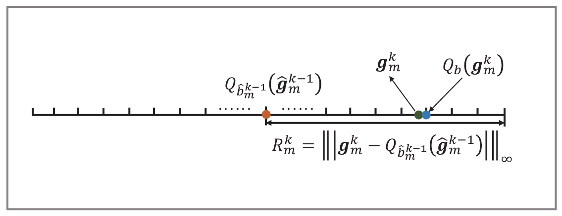
For better comparison, we adapt the quantization scheme used in LAQ algorithm(Sun et al. 2020). The scheme quantizes the difference between the new gradient $\boldsymbol{g}_{m}^{k}$ and the last quantized upload $Q_{\hat{b}_{m}^{k-1}}(\hat{\boldsymbol{g}}_{m}^{k-1})$:

With $b$ bits used for quantization, the value range of $\Delta$’s elements can be represented by a uniformly discretized grid with $2^{b}-1$ quantized values, as shown in Fig. 4. By projecting every real number in this range to the closest quantized value, $\boldsymbol{g}_{m}^{k}$ can be represented by $Q_{b}(\boldsymbol{g}_{m}^{k})$ with $b$ bits for each element instead of 32/64 bits by default.

This paper also considers random client dropout in FL, and uses $z_{m}^{k}$ to control the participation of client $m$ at iteration $k$. With a client dropping rate $p$:

If $z_{m}^{k}=1$, client $m$ drops out and fails to perform gradient computation at iteration $k$. It is obvious that with a dropping rate $p$, the percentage of active clients is approximately $1-p$ at each iteration.

With such setting, the expectation of client $m$’s upload is as follows:

where 0 is a zero vector of the same shape as $Q_{b_{m}^{k}}(\boldsymbol{g}_{m}^{k})$.

In order to get the unbaised expectation, the upload is adjusted to $Q_{b_{m}^{k}}(\boldsymbol{g}_{m}^{k})/(1-p)$, and then:

The Augmented AQG is summarized in Algorithm 2. The intuitive explanation for gradient amplification is that the loss function $f_{m}$ is smooth, which means the new update $Q_{b_{m}^{k}}(\boldsymbol{g}_{m}^{k})$ tends to be approximate to recent previous updates that may have been lost due to client dropouts.

Compared to the existing LAQ method, the proposed AQG method adjusts the number of quantization bits based on local gradient innovation adaptively. The rationale of AQG is that the proposed precision selection criterion utilizes the inherent heterogeneousness of local optimization objectives to reduce unnecessary transmission cost. Theoretical analysis in the next section will prove that AQG maintains the desired convergence properties of LAQ. Experiments show that AQG advances and fits FL better with following contributions:

• 1)

  AQG outperforms existing popular methods in terms of overall transmission bits, and achieves a more significant transmission reduction with heterogeneous data distribution compared to IID data distribution;

• 2)

  AQG is robust to a clients dropping rate up to 90$\%$, and the Augmented AQG manages to further reduce transmission overload with the presence of moderate-scale of client dropouts.

To ensure convergence, the following inequality should always hold:

Lemma 1. Under Assumption 1, (11) holds if the following three inequalities are satisfied simultaneously:

where $\rho_{1}$ and $\rho_{2}$ are constants. $\beta_{d}=\frac{1}{\alpha}\sum_{j=d}^{D}\xi_{j},\forall d\in\{1,...,D\}$. See the appendix for proof details.

It indicates that if the stepsize $\alpha$ and constants $\left\{\xi_{d}\right\}_{d=1}^{D}$ satisfy the three inequalities above, the convergence of the Lyapunov function (10) is guaranteed theoretically.

The theoretical analysis under strongly-convex loss function is based on the following assumption:
Assumption 2. Loss function $f(\boldsymbol{\theta})=\sum_{m\in\mathbb{M}}f_{m}(\boldsymbol{\theta})$ is µ-strongly convex.

Under Assumption 2, there is:

Lemma 2. Under Assumption 1 and 2, the following inequality holds:

where $c$ and $B$ are constants depending on $\mu$, $\rho_{1}$, $\rho_{2}$ and parameters involved in selection criterion (5). See the appendix for proof details.
Theorem 1. Under Assumption 1, Assumption 2 and Lemma 2, Lyapunov function and the quantization errors all converge at a linear rate:

where $\sigma\in(0,1)$ and $\tau_{b}$ is the quantization granularity with $2^{b}$ quantization levels. $P$ is a constant based on parameters in Lemma 1. See the appendix for proof details.

For experiment simplicity, logistic regression is implemented with binary classification, and a fully connected network is built for non-convex optimization. The input and output dimension of the fully connected network is 784 and 10, respectively. For both Multi-level AQG and Tow-level AQG, the quantization bit number’s upper bound $b_{max}$ is 4, the constant parameter $D$ is 10, and the weights $\left\{\xi_{d}\right\}_{d=1}^{D}=1/D$. Stepsize $\alpha$ is 0.008 for logistic regression and 0.02 for neural network.

In terms of datasets, both non-IID data distribution and IID data distribution are considered as follows:

non-IID Data Distribution: To simulate non-IID data distribution, a heterogeneous simulation dataset including 18 distributed data slices is used for logistic regression, and MNIST Dataset is used for multi-classification with the fully connected network by assigning each client with only one class of samples. The detailed description of the adopted dataset is provided in appendix. Obviously, the total client number $M$ is set as 18 for logistic regression and 10 for fully connected network with these two datasets.

IID Data Distribution: For better comparison, the same binary classification dataset used to simulate non-IID data distribution is applied to simulate IID data distribution by uniformly distributing the samples across 18 clients. For the task with fully connected network, the MNIST dataset is distributed uniformly across 10 clients. Other parameters keep the same as in non-IID data distribution.

The experiment results are shown in Table. 2. For logistic regression, all algorithms run 500 iterations. For neural network, all algorithms run 4000 iterations, and we calculate the number of iteration, communication round and transmission bit when the loss residual decreases to less than $1\times 10^{-6}$. For both tasks, the amount of bits counted for each algorithm in Table. 2 is the number of bits used to transmit one dimension of the uploaded gradient. Thus, the higher the dimension of gradient is, the more significant transmission reduction AQG brings.

With IID data distribution, training samples are distributed uniformly among clients. Fig. 5a shows that Multi-level AQG and the two-level variant of AQG both reach linear convergence rate as LAQ and QGD in strongly convex condition. Meanwhile, AQG significantly saves transmission bits compared against 4-bit LAQ and 4-bit QGD, as shown in Fig. 5c. It can be observed from Fig. 5b that the reduction of transmission bits is at the cost of a slight increase in communication rounds compared with LAQ, but it is worthy due to the significant reduction in overall transmission load.

Fig. 6 shows the results with non-convex loss function. Similar to the results with logistic regression, Multi-level AQG and two-level AQG both require fewer amount of bits to reach convergence without sacrificing the convergence properties of 4-bit LAQ and 4-bit QGD, as depicted in Fig. 6a and Fig. 6c. Meanwhile, compared with 4-bit QGD, AQG significantly reduces communication rounds to the same order of magnitude as 4-bit LAQ, as shown in Fig. 6b.

Fig. 7 and Fig. 8 verify that AQG works well with heterogeneous data distribution. Both variants of AQG manage to reduce the number of transmitted bits compared against other alternatives in both strongly convex and non-convex optimization. Meanwhile, it is obvious that experiments in non-IID data distribution benefit more with AQG compared against IID data distribution. The results are consistent with our expectation, since the idea of AQG is to utilize the inherent heterogeneousness of local optimization objectives.

In this part, we particularly focus on the setting of wireless network with mobile devices, where computation and communication are both extremely expensive, and client dropouts are frequent. Given these constraints, the Two-level AQG is applied in experiments with client dropouts as an adaptive solution for both communication and computation efficiency. Fig. 9 shows the performance of AQG with client dropping rate $p$ as 0.2, 0.5 and 0.7. Experiment results demonstrate that both AQG and Augmented AQG require fewer transmission bits compared against LAQ. Meanwhile, Augmented AQG has a stronger ability to reduce transmission bits with the presence of such moderate client dropouts.

Fig. 10 shows the performance of AQG with client dropping rate $p$ as 0.8 and 0.9. Experiments show that AQG manages to achieve stable convergence with ideal rates, and at the same time significantly reduces transmission bits even when there are only about 10$\%$ clients participating in gradient computation at each iteration. However, we notice that the augmented version of AQG fails to converge with a dropping rate higher than 0.8. It may be because when the dropping rate is too high, the unbiased estimation in Augmented AQG no longer remains accurate and even induces more noise into the training. Thus, the Augmented AQG is recommended to be applied in FL systems where the client dropping scale is moderate. Given the fact that the clients dropping rate is not likely to be so high in most practical systems, the augmented adaptive quantized gradient-based method is sufficient to address the dropping problem faced by FL.

References

• (1)
• Abadi et al. (2016) Martin Abadi, Andy Chu, Ian Goodfellow, H. Brendan McMahan, Ilya Mironov, Kunal Talwar, and Li Zhang. 2016. Deep Learning with Differential Privacy. In Proceedings of the 2016 ACM SIGSAC Conference on Computer and Communications Security (Vienna, Austria). Association for Computing Machinery, New York, NY, USA, 308–318.
• Aji and Heafield (2017) Alham Fikri Aji and Kenneth Heafield. 2017. Sparse communication for distributed gradient descent. In Proceedings of the 2017 Conference on Empirical Methods in Natural Language Processing (Copenhagen, Denmark). 440–445.
• Alistarh et al. (2017) Dan Alistarh, Demjan Grubic, Jerry Li, Ryota Tomioka, and Milan Vojnovic. 2017. QSGD: Communication-Efficient SGD via Gradient Quantization and Encoding. In Advances in Neural Information Processing Systems, Vol. 30. Curran Associates, Inc.
• Bernstein et al. (2018) Jeremy Bernstein, Yu Xiang Wang, Kamyar Azizzadenesheli, and Animashree Anandkumar. 2018. signSGD: Compressed Optimisation for Non-Convex Problems. In Proceedings of the 35th International Conference on Machine Learning, Vol. 80. PMLR, Stockholmsmässan, Stockholm Sweden, 560–569.
• Bonawitz et al. (2017) Keith Bonawitz, Vladimir Ivanov, Ben Kreuter, Antonio Marcedone, H. Brendan McMahan, Sarvar Patel, Daniel Ramage, Aaron Segal, and Karn Seth. 2017. Practical Secure Aggregation for Privacy-Preserving Machine Learning. In Proceedings of the 2017 ACM SIGSAC Conference on Computer and Communications Security (Dallas, Texas, USA). Association for Computing Machinery, New York, NY, USA, 1175–1191.
• Bouacida et al. (2020) Nader Bouacida, Jiahui Hou, Hui Zang, and Xin Liu. 2020. Adaptive Federated Dropout: Improving Communication Efficiency and Generalization for Federated Learning. arXiv preprint arXiv:2011.04050 (2020).
• Chen et al. (2018) Tianyi Chen, Georgios B Giannakis, Tao Sun, and Wotao Yin. 2018. LAG: Lazily aggregated gradient for communication-efficient distributed learning. arXiv preprint arXiv:1805.09965 (2018).
• Cheng et al. (2019) Kewei Cheng, Tao Fan, Yilun Jin, Yang Liu, Tianjian Chen, and Qiang Yang. 2019. Secureboost: A lossless federated learning framework. arXiv preprint arXiv:1901.08755 (2019).
• Diao et al. (2020) Enmao Diao, Jie Ding, and Vahid Tarokh. 2020. HeteroFL: Computation and communication efficient federated learning for heterogeneous clients. arXiv preprint arXiv:2010.01264 (2020).
• Du et al. (2020) Zhaoyang Du, Celimuge Wu, Tsutomu Yoshinaga, Kok-Lim Alvin Yau, Yusheng Ji, and Jie Li. 2020. Federated learning for vehicular internet of things: Recent advances and open issues. IEEE Open Journal of the Computer Society 1 (2020), 45–61.
• Güvenir et al. (1998) HA Güvenir, G. Demir?Z, and N. ?Lter. 1998. Learning differential diagnosis of erythemato-squamous diseases using voting feature intervals. Artificial Intelligence in Medicine 13, 3 (1998), 147–165.
• Hard et al. (2018) Andrew Hard, Kanishka Rao, Rajiv Mathews, Swaroop Ramaswamy, Françoise Beaufays, Sean Augenstein, Hubert Eichner, Chloé Kiddon, and Daniel Ramage. 2018. Federated learning for mobile keyboard prediction. arXiv preprint arXiv:1811.03604 (2018).
• He et al. (2020) Yinghui He, Jinke Ren, Guanding Yu, and Jiantao Yuan. 2020. Resource Allocation for Wireless Federated Edge Learning based on Data Importance. In GLOBECOM 2020-2020 IEEE Global Communications Conference. IEEE, 1–6.
• Kaissis et al. (2020) Georgios A Kaissis, Marcus R Makowski, Daniel Rückert, and Rickmer F Braren. 2020. Secure, privacy-preserving and federated machine learning in medical imaging. Nature Machine Intelligence 2, 6 (2020), 305–311.
• Kohavi (1997) R. Kohavi. 1997. Scaling Up the Accuracy of Naive-Bayes Classifiers: a Decision-Tree Hybrid. 96 (1997), 202–207.
• Lin et al. (2018) Yujun Lin, Song Han, Huizi Mao, Yu Wang, and William J Dally. 2018. Deep gradient compression: Reducing the communication bandwidth for distributed training. In Proceedings of International Conference on Learning Representations (Vancouver, Canada).
• Liu et al. (2020a) Yang Liu, Anbu Huang, Yun Luo, He Huang, Youzhi Liu, Yuanyuan Chen, Lican Feng, Tianjian Chen, Han Yu, and Qiang Yang. 2020a. Fedvision: An online visual object detection platform powered by federated learning. In Proceedings of the AAAI Conference on Artificial Intelligence, Vol. 34. 13172–13179.
• Liu et al. (2020b) Yang Liu, Yan Kang, Chaoping Xing, Tianjian Chen, and Qiang Yang. 2020b. A secure federated transfer learning framework. IEEE Intelligent Systems 35, 4 (2020), 70–82.
• McMahan et al. (2017) Brendan McMahan, Eider Moore, Daniel Ramage, Seth Hampson, and Blaise Aguera y Arcas. 2017. Communication-Efficient Learning of Deep Networks from Decentralized Data. In Proceedings of the 20th International Conference on Artificial Intelligence and Statistics, Vol. 54. PMLR, Fort Lauderdale, FL, USA, 1273–1282.
• Nishio and Yonetani (2019) Takayuki Nishio and Ryo Yonetani. 2019. Client selection for federated learning with heterogeneous resources in mobile edge. In ICC 2019-2019 IEEE International Conference on Communications (ICC). IEEE, 1–7.
• Seide et al. (2014) Frank Seide, Hao Fu, Jasha Droppo, Gang Li, and Dong Yu. 2014. 1-bit stochastic gradient descent and its application to data-parallel distributed training of speech DNNs. In INTERSPEECH. 1058–1062.
• Sigillito et al. (1989) V. G. Sigillito, S. P. Wing, L. V. Hutton, and K. B. Baker. 1989. Classification of radar returns from the ionosphere using neural networks. Johns Hopkins APL Technical Digest 10, 3 (1989), 262–266.
• Singh et al. (2020) Navjot Singh, Deepesh Data, Jemin George, and Suhas Diggavi. 2020. SPARQ-SGD: Event-Triggered and Compressed Communication in Decentralized Optimization. In 2020 59th IEEE Conference on Decision and Control (CDC). IEEE, 3449–3456.
• Stich et al. (2018) Sebastian U. Stich, Jean-Baptiste Cordonnier, and Martin Jaggi. 2018. Sparsified SGD with Memory. In Proceedings of the 32nd International Conference on Neural Information Processing Systems (Montréal, Canada). Curran Associates Inc., Red Hook, NY, USA, 4452–4463.
• Sun et al. (2020) J. Sun, T. Chen, G. B. Giannakis, Q. Yang, and Z. Yang. 2020. Lazily Aggregated Quantized Gradient Innovation for Communication-Efficient Federated Learning. IEEE Transactions on Pattern Analysis and Machine Intelligence (2020), 1–1. https://doi.org/10.1109/TPAMI.2020.3033286
• Wang et al. (2018) Hongyi Wang, Scott Sievert, Zachary Charles, Shengchao Liu, Stephen Wright, and Dimitris Papailiopoulos. 2018. ATOMO: Communication-Efficient Learning via Atomic Sparsification. In Proceedings of the 32nd International Conference on Neural Information Processing Systems (Montréal, Canada) (NIPS’18). Curran Associates Inc., Red Hook, NY, USA, 9872–9883.
• Wangni et al. (2018) Jianqiao Wangni, Jialei Wang, Ji Liu, and Tong Zhang. 2018. Gradient Sparsification for Communication-Efficient Distributed Optimization. In Proceedings of the 32nd International Conference on Neural Information Processing Systems (Montréal, Canada). Curran Associates Inc., Red Hook, NY, USA, 1306–1316.
• Yang et al. (2019) Qiang Yang, Yang Liu, Tianjian Chen, and Yongxin Tong. 2019. Federated machine learning: Concept and applications. ACM Transactions on Intelligent Systems and Technology (TIST) 10, 2 (2019), 1–19.
• Zhu et al. (2020) Tongxin Zhu, Jianzhong Li, Zhipeng Cai, Yingshu Li, and Hong Gao. 2020. Computation scheduling for wireless powered mobile edge computing networks. In IEEE INFOCOM 2020-IEEE Conference on Computer Communications. IEEE, 596–605.
Appendix A Mathematical Proof
A.1. Proof of Lemma 1
In AQG:
∑m=1MQb^mk​(𝒈^mk)=∑b=1bm​a​x∑m∈𝕄bkQb^mk​(𝒈^mk)+∑m∈𝕄0kQb^mk−1​(𝒈^mk−1)\displaystyle\sum_{m=1}^{M}Q_{\hat{b}_{m}^{k}}(\hat{\boldsymbol{g}}_{m}^{k})=\sum_{b=1}^{b_{max}}\sum_{m\in\mathbb{M}_{b}^{k}}Q_{\hat{b}_{m}^{k}}(\hat{\boldsymbol{g}}_{m}^{k})+\sum_{m\in\mathbb{M}_{0}^{k}}Q_{\hat{b}_{m}^{k-1}}(\hat{\boldsymbol{g}}_{m}^{k-1})
(16) =∑m=1MQbm​a​x​(𝒈^mk)+∑b=1bm​a​x∑m∈𝕄bk[Qb^mk​(𝒈^mk)−Qbm​a​x​(𝒈^mk)]+∑m∈𝕄0k[Qb^mk−1​(𝒈^mk−1)−Qbm​a​x​(𝒈^mk)]\displaystyle=\sum_{m=1}^{M}Q_{b_{max}}(\hat{\boldsymbol{g}}_{m}^{k})+\sum_{b=1}^{b_{max}}\sum_{m\in\mathbb{M}_{b}^{k}}[Q_{\hat{b}_{m}^{k}}(\hat{\boldsymbol{g}}_{m}^{k})-Q_{b_{max}}(\hat{\boldsymbol{g}}_{m}^{k})]+\sum_{m\in\mathbb{M}_{0}^{k}}[Q_{\hat{b}_{m}^{k-1}}(\hat{\boldsymbol{g}}_{m}^{k-1})-Q_{b_{max}}(\hat{\boldsymbol{g}}_{m}^{k})]
From the update rule of AQG:
(17) 𝜽k+1−𝜽k=−α∑m=1MQb^mk(𝒈^mk)\boldsymbol{\theta}^{k+1}-\boldsymbol{\theta}^{k}=-\alpha\sum_{m=1}^{M}Q_{\hat{b}_{m}^{k}}(\hat{\boldsymbol{g}}_{m}^{k})
From the definition of quantization error:
(18) ∑m=1MQbm​a​x​(𝒈^mk)=∇f​(𝜽k)−∑m=1Mεbm​a​x​(𝒈^mk)\sum_{m=1}^{M}Q_{b_{max}}(\hat{\boldsymbol{g}}_{m}^{k})=\nabla f(\boldsymbol{\theta}^{k})-\sum_{m=1}^{M}\varepsilon_{b_{max}}(\hat{\boldsymbol{g}}_{m}^{k})
With inequality ⟨𝒂,𝒃⟩≤12​ρ​‖𝒂‖22+12​ρ​‖𝒃‖22\left\langle\boldsymbol{a},\boldsymbol{b}\right\rangle\leq\frac{1}{2}\rho\left\|\boldsymbol{a}\right\|_{2}^{2}+\frac{1}{2\rho}\left\|\boldsymbol{b}\right\|_{2}^{2} and (18):
−α⁡⟨∇f​(𝜽k),∑m=1MQbm​a​x​(𝒈^mk)⟩=−α⁡⟨∇f​(𝜽k),∇f​(𝜽k)−∑m=1Mεbm​a​x​(𝒈^mk)⟩\displaystyle-\alpha\left\langle\nabla f(\boldsymbol{\theta}^{k}),\sum_{m=1}^{M}Q_{b_{max}}(\hat{\boldsymbol{g}}_{m}^{k})\right\rangle=-\alpha\left\langle\nabla f(\boldsymbol{\theta}^{k}),\nabla f(\boldsymbol{\theta}^{k})-\sum_{m=1}^{M}\varepsilon_{b_{max}}(\hat{\boldsymbol{g}}_{m}^{k})\right\rangle
=−α​‖∇f​(𝜽k)‖22+α⁡⟨∇f​(𝜽k),∑m=1Mεbm​a​x​(𝒈^mk)⟩\displaystyle=-\alpha\left\|\nabla f(\boldsymbol{\theta}^{k})\right\|_{2}^{2}+\alpha\left\langle\nabla f(\boldsymbol{\theta}^{k}),\sum_{m=1}^{M}\varepsilon_{b_{max}}(\hat{\boldsymbol{g}}_{m}^{k})\right\rangle
(19) ≤−α​‖∇f​(𝜽k)‖22+α​ρ12​‖∇f​(𝜽k)‖22+α2​ρ1​‖∑m=1Mεbm​a​x​(𝒈^mk)‖22\displaystyle\leq-\alpha\left\|\nabla f(\boldsymbol{\theta}^{k})\right\|_{2}^{2}+\frac{\alpha\rho_{1}}{2}\left\|\nabla f(\boldsymbol{\theta}^{k})\right\|_{2}^{2}+\frac{\alpha}{2\rho_{1}}\left\|\sum_{m=1}^{M}\varepsilon_{b_{max}}(\hat{\boldsymbol{g}}_{m}^{k})\right\|_{2}^{2}
Under Assumption 1:
f⁡(𝜽k+1)−f⁡(𝜽k)≤⟨∇f​(𝜽k),𝜽k+1−𝜽k⟩+L2​‖𝜽k+1−𝜽k‖22\displaystyle f(\boldsymbol{\theta}^{k+1})-f(\boldsymbol{\theta}^{k})\leq\left\langle\nabla f(\boldsymbol{\theta}^{k}),\boldsymbol{\theta}^{k+1}-\boldsymbol{\theta}^{k}\right\rangle+\frac{L}{2}\left\|\boldsymbol{\theta}^{k+1}-\boldsymbol{\theta}^{k}\right\|_{2}^{2}
=⟨∇f(𝜽k),−α∑m=1MQb^mk(𝒈^mk)⟩+L2‖𝜽k+1−𝜽k‖22\displaystyle=\left\langle\nabla f(\boldsymbol{\theta}^{k}),-\alpha\sum_{m=1}^{M}Q_{\hat{b}_{m}^{k}}(\hat{\boldsymbol{g}}_{m}^{k})\right\rangle+\frac{L}{2}\left\|\boldsymbol{\theta}^{k+1}-\boldsymbol{\theta}^{k}\right\|_{2}^{2}
=⟨∇f(𝜽k),−α∑m=1MQbm​a​x(𝒈^mk)⟩+L2‖𝜽k+1−𝜽k‖22\displaystyle=\left\langle\nabla f(\boldsymbol{\theta}^{k}),-\alpha\sum_{m=1}^{M}Q_{b_{max}}(\hat{\boldsymbol{g}}_{m}^{k})\right\rangle+\frac{L}{2}\left\|\boldsymbol{\theta}^{k+1}-\boldsymbol{\theta}^{k}\right\|_{2}^{2}
+⟨∇f​(𝜽k),−α⁡{∑b=1bm​a​x∑m∈𝕄bk[Qb^mk​(𝒈^mk)−Qbm​a​x​(𝒈^mk)]+∑m∈𝕄0k[Qb^mk−1​(𝒈^mk−1)−Qbm​a​x​(𝒈^mk)]}⟩\displaystyle+\left\langle\nabla f(\boldsymbol{\theta}^{k}),-\alpha\left\{\sum_{b=1}^{b_{max}}\sum_{m\in\mathbb{M}_{b}^{k}}[Q_{\hat{b}_{m}^{k}}(\hat{\boldsymbol{g}}_{m}^{k})-Q_{b_{max}}(\hat{\boldsymbol{g}}_{m}^{k})]+\sum_{m\in\mathbb{M}_{0}^{k}}[Q_{\hat{b}_{m}^{k-1}}(\hat{\boldsymbol{g}}_{m}^{k-1})-Q_{b_{max}}(\hat{\boldsymbol{g}}_{m}^{k})]\right\}\right\rangle
≤⟨∇f(𝜽k),−α∑m=1MQbm​a​x(𝒈^mk)⟩+L2‖𝜽k+1−𝜽k‖22+α2‖∇f(𝜽k)‖22\displaystyle\leq\left\langle\nabla f(\boldsymbol{\theta}^{k}),-\alpha\sum_{m=1}^{M}Q_{b_{max}}(\hat{\boldsymbol{g}}_{m}^{k})\right\rangle+\frac{L}{2}\left\|\boldsymbol{\theta}^{k+1}-\boldsymbol{\theta}^{k}\right\|_{2}^{2}+\frac{\alpha}{2}\left\|\nabla f(\boldsymbol{\theta}^{k})\right\|_{2}^{2}
(20) +α2​‖∑b=1bm​a​x∑m∈𝕄bk[Qb^mk​(𝒈^mk)−Qbm​a​x​(𝒈^mk)]+∑m∈𝕄0k[Qb^mk−1​(𝒈^mk−1)−Qbm​a​x​(𝒈^mk)]‖22\displaystyle+\frac{\alpha}{2}\left\|\sum_{b=1}^{b_{max}}\sum_{m\in\mathbb{M}_{b}^{k}}[Q_{\hat{b}_{m}^{k}}(\hat{\boldsymbol{g}}_{m}^{k})-Q_{b_{max}}(\hat{\boldsymbol{g}}_{m}^{k})]+\sum_{m\in\mathbb{M}_{0}^{k}}[Q_{\hat{b}_{m}^{k-1}}(\hat{\boldsymbol{g}}_{m}^{k-1})-Q_{b_{max}}(\hat{\boldsymbol{g}}_{m}^{k})]\right\|_{2}^{2}
The Lyapunov function of AQG is defined as:
(21) 𝕍⁡(𝜽k)=f⁡(𝜽k)−f⁡(𝜽∗)+∑d=1D∑j=dDξjα​‖𝜽k+1−d−𝜽k−d‖22\mathbb{V}(\boldsymbol{\theta}^{k})=f(\boldsymbol{\theta}^{k})-f(\boldsymbol{\theta}^{*})+\sum_{d=1}^{D}\sum_{j=d}^{D}\frac{\xi_{j}}{\alpha}\left\|\boldsymbol{\theta}^{k+1-d}-\boldsymbol{\theta}^{k-d}\right\|_{2}^{2}
Let βd=1α​∑j=dDξj,∀d∈{1,…,D}\beta_{d}=\frac{1}{\alpha}\sum_{j=d}^{D}\xi_{j},\forall d\in\{1,...,D\}, then:
(22) 𝕍⁡(𝜽k)=f⁡(𝜽k)−f⁡(𝜽∗)+∑d=1Dβd​‖𝜽k+1−d−𝜽k−d‖22\mathbb{V}(\boldsymbol{\theta}^{k})=f(\boldsymbol{\theta}^{k})-f(\boldsymbol{\theta}^{*})+\sum_{d=1}^{D}\beta_{d}\left\|\boldsymbol{\theta}^{k+1-d}-\boldsymbol{\theta}^{k-d}\right\|_{2}^{2}
Thus,
𝕍⁡(𝜽k+1)−𝕍⁡(𝜽k)=f⁡(𝜽k+1)−f⁡(𝜽k)+∑d=1Dβd​‖𝜽k+1−(d−1)−𝜽k−(d−1)‖22−∑d=1Dβd​‖𝜽k+1−d−𝜽k−d‖22\displaystyle\mathbb{V}(\boldsymbol{\theta}^{k+1})-\mathbb{V}(\boldsymbol{\theta}^{k})=f(\boldsymbol{\theta}^{k+1})-f(\boldsymbol{\theta}^{k})+\sum_{d=1}^{D}\beta_{d}\left\|\boldsymbol{\theta}^{k+1-(d-1)}-\boldsymbol{\theta}^{k-(d-1)}\right\|_{2}^{2}-\sum_{d=1}^{D}\beta_{d}\left\|\boldsymbol{\theta}^{k+1-d}-\boldsymbol{\theta}^{k-d}\right\|_{2}^{2}
=f⁡(𝜽k+1)−f⁡(𝜽k)+β1​‖𝜽k+1−𝜽k‖22+∑d=1D−1(βd+1−βd)​‖𝜽k+1−d−𝜽k−d‖22−βD​‖𝜽k+1−D−𝜽k−D‖22\displaystyle=f(\boldsymbol{\theta}^{k+1})-f(\boldsymbol{\theta}^{k})+\beta_{1}\left\|\boldsymbol{\theta}^{k+1}-\boldsymbol{\theta}^{k}\right\|_{2}^{2}+\sum_{d=1}^{D-1}(\beta_{d+1}-\beta_{d})\left\|\boldsymbol{\theta}^{k+1-d}-\boldsymbol{\theta}^{k-d}\right\|_{2}^{2}-\beta_{D}\left\|\boldsymbol{\theta}^{k+1-D}-\boldsymbol{\theta}^{k-D}\right\|_{2}^{2}
≤−α⁡⟨∇f​(𝜽k),∑m=1MQbm​a​x​(𝒈^mk)⟩+α2​‖∇f​(𝜽k)‖22\displaystyle\leq-\alpha\left\langle\nabla f(\boldsymbol{\theta}^{k}),\sum_{m=1}^{M}Q_{b_{max}}(\hat{\boldsymbol{g}}_{m}^{k})\right\rangle+\frac{\alpha}{2}\left\|\nabla f(\boldsymbol{\theta}^{k})\right\|_{2}^{2}
+α2​‖∑b=1bm​a​x∑m∈𝕄bk[Qb^mk​(𝒈^mk)−Qbm​a​x​(𝒈^mk)]+∑m∈𝕄0k[Qb^mk−1​(𝒈^mk−1)−Qbm​a​x​(𝒈^mk)]‖22\displaystyle+\frac{\alpha}{2}\left\|\sum_{b=1}^{b_{max}}\sum_{m\in\mathbb{M}_{b}^{k}}[Q_{\hat{b}_{m}^{k}}(\hat{\boldsymbol{g}}_{m}^{k})-Q_{b_{max}}(\hat{\boldsymbol{g}}_{m}^{k})]+\sum_{m\in\mathbb{M}_{0}^{k}}[Q_{\hat{b}_{m}^{k-1}}(\hat{\boldsymbol{g}}_{m}^{k-1})-Q_{b_{max}}(\hat{\boldsymbol{g}}_{m}^{k})]\right\|_{2}^{2}
(23) +(L2+β1)​‖𝜽k+1−𝜽k‖22+∑d=1D−1(βd+1−βd)​‖𝜽k+1−d−𝜽k−d‖22−βD​‖𝜽k+1−D−𝜽k−D‖22\displaystyle+(\frac{L}{2}+\beta_{1})\left\|\boldsymbol{\theta}^{k+1}-\boldsymbol{\theta}^{k}\right\|_{2}^{2}+\sum_{d=1}^{D-1}(\beta_{d+1}-\beta_{d})\left\|\boldsymbol{\theta}^{k+1-d}-\boldsymbol{\theta}^{k-d}\right\|_{2}^{2}-\beta_{D}\left\|\boldsymbol{\theta}^{k+1-D}-\boldsymbol{\theta}^{k-D}\right\|_{2}^{2}
=−α⁡⟨∇f​(𝜽k),∑m=1MQbm​a​x​(𝒈^mk)⟩+α2​‖∇f​(𝜽k)‖22+∑d=1D−1(βd+1−βd)​‖𝜽k+1−d−𝜽k−d‖22−βD​‖𝜽k+1−D−𝜽k−D‖22\displaystyle=-\alpha\left\langle\nabla f(\boldsymbol{\theta}^{k}),\sum_{m=1}^{M}Q_{b_{max}}(\hat{\boldsymbol{g}}_{m}^{k})\right\rangle+\frac{\alpha}{2}\left\|\nabla f(\boldsymbol{\theta}^{k})\right\|_{2}^{2}+\sum_{d=1}^{D-1}(\beta_{d+1}-\beta_{d})\left\|\boldsymbol{\theta}^{k+1-d}-\boldsymbol{\theta}^{k-d}\right\|_{2}^{2}-\beta_{D}\left\|\boldsymbol{\theta}^{k+1-D}-\boldsymbol{\theta}^{k-D}\right\|_{2}^{2}
+(L2+β1)​‖α⁡{∑m=1MQbm​a​x​(𝒈^mk)+∑b=1bm​a​x∑m∈𝕄bk[Qb^mk​(𝒈^mk)−Qbm​a​x​(𝒈^mk)]+∑m∈𝕄0k[Qb^mk−1​(𝒈^mk−1)−Qbm​a​x​(𝒈^mk)]}‖22\displaystyle+(\frac{L}{2}+\beta_{1})\left\|\alpha\left\{\sum_{m=1}^{M}Q_{b_{max}}(\hat{\boldsymbol{g}}_{m}^{k})+\sum_{b=1}^{b_{max}}\sum_{m\in\mathbb{M}_{b}^{k}}[Q_{\hat{b}_{m}^{k}}(\hat{\boldsymbol{g}}_{m}^{k})-Q_{b_{max}}(\hat{\boldsymbol{g}}_{m}^{k})]+\sum_{m\in\mathbb{M}_{0}^{k}}[Q_{\hat{b}_{m}^{k-1}}(\hat{\boldsymbol{g}}_{m}^{k-1})-Q_{b_{max}}(\hat{\boldsymbol{g}}_{m}^{k})]\right\}\right\|_{2}^{2}
(24) +α2​‖∑b=1bm​a​x∑m∈𝕄bk[Qb^mk​(𝒈^mk)−Qbm​a​x​(𝒈^mk)]+∑m∈𝕄0k[Qb^mk−1​(𝒈^mk−1)−Qbm​a​x​(𝒈^mk)]‖22\displaystyle+\frac{\alpha}{2}\left\|\sum_{b=1}^{b_{max}}\sum_{m\in\mathbb{M}_{b}^{k}}[Q_{\hat{b}_{m}^{k}}(\hat{\boldsymbol{g}}_{m}^{k})-Q_{b_{max}}(\hat{\boldsymbol{g}}_{m}^{k})]+\sum_{m\in\mathbb{M}_{0}^{k}}[Q_{\hat{b}_{m}^{k-1}}(\hat{\boldsymbol{g}}_{m}^{k-1})-Q_{b_{max}}(\hat{\boldsymbol{g}}_{m}^{k})]\right\|_{2}^{2}
From Young’s Equality ‖a+𝐛‖22≤(1+ρ)​‖a‖22+(1+ρ−1)​‖b‖22\left\|\textbf{a}+\mathbf{b}\right\|_{2}^{2}\leq(1+\rho)\left\|\textbf{a}\right\|_{2}^{2}+(1+\rho^{-1})\left\|\textbf{b}\right\|_{2}^{2}, there is:
(L2+β1)​‖α⁡{∑m=1MQbm​a​x​(𝒈^mk)+∑b=1bm​a​x∑m∈𝕄bk[Qb^mk​(𝒈^mk)−Qbm​a​x​(𝒈^mk)]+∑m∈𝕄0k[Qb^mk−1​(𝒈^mk−1)−Qbm​a​x​(𝒈^mk)]}‖22\displaystyle(\frac{L}{2}+\beta_{1})\left\|\alpha\left\{\sum_{m=1}^{M}Q_{b_{max}}(\hat{\boldsymbol{g}}_{m}^{k})+\sum_{b=1}^{b_{max}}\sum_{m\in\mathbb{M}_{b}^{k}}[Q_{\hat{b}_{m}^{k}}(\hat{\boldsymbol{g}}_{m}^{k})-Q_{b_{max}}(\hat{\boldsymbol{g}}_{m}^{k})]+\sum_{m\in\mathbb{M}_{0}^{k}}[Q_{\hat{b}_{m}^{k-1}}(\hat{\boldsymbol{g}}_{m}^{k-1})-Q_{b_{max}}(\hat{\boldsymbol{g}}_{m}^{k})]\right\}\right\|_{2}^{2}
≤(L2+β1)​(1+ρ2−1)​α2​‖∑b=1bm​a​x∑m∈𝕄bk[Qb^mk​(𝒈^mk)−Qbm​a​x​(𝒈^mk)]+∑m∈𝕄0k[Qb^mk−1​(𝒈^mk−1)−Qbm​a​x​(𝒈^mk)]‖22\displaystyle\leq(\frac{L}{2}+\beta_{1})(1+\rho_{2}^{-1})\alpha^{2}\left\|\sum_{b=1}^{b_{max}}\sum_{m\in\mathbb{M}_{b}^{k}}[Q_{\hat{b}_{m}^{k}}(\hat{\boldsymbol{g}}_{m}^{k})-Q_{b_{max}}(\hat{\boldsymbol{g}}_{m}^{k})]+\sum_{m\in\mathbb{M}_{0}^{k}}[Q_{\hat{b}_{m}^{k-1}}(\hat{\boldsymbol{g}}_{m}^{k-1})-Q_{b_{max}}(\hat{\boldsymbol{g}}_{m}^{k})]\right\|_{2}^{2}
(25) +(L2+β1)​(1+ρ2)​α2​‖∑m=1MQbm​a​x​(𝒈^mk)‖22\displaystyle+(\frac{L}{2}+\beta_{1})(1+\rho_{2})\alpha^{2}\left\|\sum_{m=1}^{M}Q_{b_{max}}(\hat{\boldsymbol{g}}_{m}^{k})\right\|_{2}^{2}
From ‖∑i=1n𝒂i‖22≤n​∑i=1n‖𝒂i‖22\left\|\sum_{i=1}^{n}\boldsymbol{a}_{i}\right\|_{2}^{2}\leq n\sum_{i=1}^{n}\left\|\boldsymbol{a}_{i}\right\|_{2}^{2}, there is:
‖∑b=1bm​a​x∑m∈𝕄bk[Qb^mk​(𝒈^mk)−Qbm​a​x​(𝒈^mk)]+∑m∈𝕄0k[Qb^mk−1​(𝒈^mk−1)−Qbm​a​x​(𝒈^mk)]‖22\displaystyle\left\|\sum_{b=1}^{b_{max}}\sum_{m\in\mathbb{M}_{b}^{k}}[Q_{\hat{b}_{m}^{k}}(\hat{\boldsymbol{g}}_{m}^{k})-Q_{b_{max}}(\hat{\boldsymbol{g}}_{m}^{k})]+\sum_{m\in\mathbb{M}_{0}^{k}}[Q_{\hat{b}_{m}^{k-1}}(\hat{\boldsymbol{g}}_{m}^{k-1})-Q_{b_{max}}(\hat{\boldsymbol{g}}_{m}^{k})]\right\|_{2}^{2}
≤M​∑b=1bm​a​x∑m∈𝕄bk‖Qb^mk​(𝒈^mk)−Qbm​a​x​(𝒈^mk)‖22+M​∑m∈𝕄0k‖Qb^mk−1​(𝒈^mk−1)−Qbm​a​x​(𝒈^mk)‖22\displaystyle\leq M\sum_{b=1}^{b_{max}}\sum_{m\in\mathbb{M}_{b}^{k}}\left\|Q_{\hat{b}_{m}^{k}}(\hat{\boldsymbol{g}}_{m}^{k})-Q_{b_{max}}(\hat{\boldsymbol{g}}_{m}^{k})\right\|_{2}^{2}+M\sum_{m\in\mathbb{M}_{0}^{k}}\left\|Q_{\hat{b}_{m}^{k-1}}(\hat{\boldsymbol{g}}_{m}^{k-1})-Q_{b_{max}}(\hat{\boldsymbol{g}}_{m}^{k})\right\|_{2}^{2}
(26) =2​M​∑b=1bm​a​x∑m∈𝕄bk‖εb^mk​(𝒈^mk)‖22+2​M​∑b=1bm​a​x∑m∈𝕄bk‖εbm​a​x​(𝒈^mk)‖22+M​∑m∈𝕄0k‖Qb^mk−1​(𝒈^mk−1)−Qbm​a​x​(𝒈^mk)‖22\displaystyle=2M\sum_{b=1}^{b_{max}}\sum_{m\in\mathbb{M}_{b}^{k}}\left\|\varepsilon_{\hat{b}_{m}^{k}}(\hat{\boldsymbol{g}}_{m}^{k})\right\|_{2}^{2}+2M\sum_{b=1}^{b_{max}}\sum_{m\in\mathbb{M}_{b}^{k}}\left\|\varepsilon_{b_{max}}(\hat{\boldsymbol{g}}_{m}^{k})\right\|_{2}^{2}+M\sum_{m\in\mathbb{M}_{0}^{k}}\left\|Q_{\hat{b}_{m}^{k-1}}(\hat{\boldsymbol{g}}_{m}^{k-1})-Q_{b_{max}}(\hat{\boldsymbol{g}}_{m}^{k})\right\|_{2}^{2}
With (25) and (26):
𝕍⁡(𝜽k+1)−𝕍⁡(𝜽k)≤−α⁡⟨∇f​(𝜽k),∑m=1MQbm​a​x​(𝒈^mk)⟩+α2​‖∇f​(𝜽k)‖22\displaystyle\mathbb{V}(\boldsymbol{\theta}^{k+1})-\mathbb{V}(\boldsymbol{\theta}^{k})\leq-\alpha\left\langle\nabla f(\boldsymbol{\theta}^{k}),\sum_{m=1}^{M}Q_{b_{max}}(\hat{\boldsymbol{g}}_{m}^{k})\right\rangle+\frac{\alpha}{2}\left\|\nabla f(\boldsymbol{\theta}^{k})\right\|_{2}^{2}
+(L2+β1)​(1+ρ2)​α2​‖∑m=1MQbm​a​x​(𝒈^mk)‖22+∑d=1D−1(βd+1−βd)​‖𝜽k+1−d−𝜽k−d‖22−βD​‖𝜽k+1−D−𝜽k−D‖22\displaystyle+(\frac{L}{2}+\beta_{1})(1+\rho_{2})\alpha^{2}\left\|\sum_{m=1}^{M}Q_{b_{max}}(\hat{\boldsymbol{g}}_{m}^{k})\right\|_{2}^{2}+\sum_{d=1}^{D-1}(\beta_{d+1}-\beta_{d})\left\|\boldsymbol{\theta}^{k+1-d}-\boldsymbol{\theta}^{k-d}\right\|_{2}^{2}-\beta_{D}\left\|\boldsymbol{\theta}^{k+1-D}-\boldsymbol{\theta}^{k-D}\right\|_{2}^{2}
+[α2+(L2+β1)​(1+ρ2−1)​α2]​‖∑b=1bm​a​x∑m∈𝕄bk[Qb^mk​(𝒈^mk)−Qbm​a​x​(𝒈^mk)]+∑m∈𝕄0k[Qb^mk−1​(𝒈^mk−1)−Qbm​a​x​(𝒈^mk)]‖22\displaystyle+[\frac{\alpha}{2}+(\frac{L}{2}+\beta_{1})(1+\rho_{2}^{-1})\alpha^{2}]\left\|\sum_{b=1}^{b_{max}}\sum_{m\in\mathbb{M}_{b}^{k}}[Q_{\hat{b}_{m}^{k}}(\hat{\boldsymbol{g}}_{m}^{k})-Q_{b_{max}}(\hat{\boldsymbol{g}}_{m}^{k})]+\sum_{m\in\mathbb{M}_{0}^{k}}[Q_{\hat{b}_{m}^{k-1}}(\hat{\boldsymbol{g}}_{m}^{k-1})-Q_{b_{max}}(\hat{\boldsymbol{g}}_{m}^{k})]\right\|_{2}^{2}
≤−α⁡⟨∇f​(𝜽k),∑m=1MQbm​a​x​(𝒈^mk)⟩+α2​‖∇f​(𝜽k)‖22+(L2+β1)​(1+ρ2)​α2​‖∑m=1MQbm​a​x​(𝒈^mk)‖22\displaystyle\leq-\alpha\left\langle\nabla f(\boldsymbol{\theta}^{k}),\sum_{m=1}^{M}Q_{b_{max}}(\hat{\boldsymbol{g}}_{m}^{k})\right\rangle+\frac{\alpha}{2}\left\|\nabla f(\boldsymbol{\theta}^{k})\right\|_{2}^{2}+(\frac{L}{2}+\beta_{1})(1+\rho_{2})\alpha^{2}\left\|\sum_{m=1}^{M}Q_{b_{max}}(\hat{\boldsymbol{g}}_{m}^{k})\right\|_{2}^{2}
+∑d=1D−1(βd+1−βd)‖𝜽k+1−d−𝜽k−d‖22−βD‖𝜽k+1−D−𝜽k−D‖22\displaystyle+\sum_{d=1}^{D-1}(\beta_{d+1}-\beta_{d})\left\|\boldsymbol{\theta}^{k+1-d}-\boldsymbol{\theta}^{k-d}\right\|_{2}^{2}-\beta_{D}\left\|\boldsymbol{\theta}^{k+1-D}-\boldsymbol{\theta}^{k-D}\right\|_{2}^{2}
+2​[α2+(L2+β1)​(1+ρ2−1)​α2]​M​(∑b=1bm​a​x∑m∈𝕄bk‖εb^mk​(𝒈^mk)‖22+∑b=1bm​a​x∑m∈𝕄bk‖εbm​a​x​(𝒈^mk)‖22)\displaystyle+2[\frac{\alpha}{2}+(\frac{L}{2}+\beta_{1})(1+\rho_{2}^{-1})\alpha^{2}]M(\sum_{b=1}^{b_{max}}\sum_{m\in\mathbb{M}_{b}^{k}}\left\|\varepsilon_{\hat{b}_{m}^{k}}(\hat{\boldsymbol{g}}_{m}^{k})\right\|_{2}^{2}+\sum_{b=1}^{b_{max}}\sum_{m\in\mathbb{M}_{b}^{k}}\left\|\varepsilon_{b_{max}}(\hat{\boldsymbol{g}}_{m}^{k})\right\|_{2}^{2})
(27) +[α2+(L2+β1)(1+ρ2−1)α2]M∑m∈𝕄0k‖Qb^mk−1(𝒈^mk−1)−Qbm​a​x(𝒈^mk)‖22\displaystyle+[\frac{\alpha}{2}+(\frac{L}{2}+\beta_{1})(1+\rho_{2}^{-1})\alpha^{2}]M\sum_{m\in\mathbb{M}_{0}^{k}}\left\|Q_{\hat{b}_{m}^{k-1}}(\hat{\boldsymbol{g}}_{m}^{k-1})-Q_{b_{max}}(\hat{\boldsymbol{g}}_{m}^{k})\right\|_{2}^{2}
With the precision selection criterion (5):
M​∑m∈𝕄0k‖Qb^mk−1​(𝒈^mk−1)−Qbm​a​x​(𝒈mk)‖22\displaystyle M\sum_{m\in\mathbb{M}_{0}^{k}}\left\|Q_{\hat{b}_{m}^{k-1}}(\hat{\boldsymbol{g}}_{m}^{k-1})-Q_{b_{max}}(\boldsymbol{g}_{m}^{k})\right\|_{2}^{2}
(28) ≤M2α2​M2​∑d=1Dξd​‖𝜽k+1−d−𝜽k−d‖22+3​M​∑m∈𝕄0k(‖εbm​a​x​(𝒈^mk−1)‖22+‖εbm​a​x​(𝒈mk)‖22)\displaystyle\leq\frac{M^{2}}{\alpha^{2}M^{2}}\sum_{d=1}^{D}\xi_{d}\left\|\boldsymbol{\theta}^{k+1-d}-\boldsymbol{\theta}^{k-d}\right\|_{2}^{2}+3M\sum_{m\in\mathbb{M}_{0}^{k}}(\left\|\varepsilon_{b_{max}}(\hat{\boldsymbol{g}}_{m}^{k-1})\right\|_{2}^{2}+\left\|\varepsilon_{b_{max}}({\boldsymbol{g}}_{m}^{k})\right\|_{2}^{2})
𝕍⁡(𝜽k+1)−𝕍⁡(𝜽k)\displaystyle\mathbb{V}(\boldsymbol{\theta}^{k+1})-\mathbb{V}(\boldsymbol{\theta}^{k})
+[α2+(L2+β1)(1+ρ2−1)α2]1α2∑d=1Dξd‖𝜽k+1−d−𝜽k−d‖22\displaystyle+[\frac{\alpha}{2}+(\frac{L}{2}+\beta_{1})(1+\rho_{2}^{-1})\alpha^{2}]\frac{1}{\alpha^{2}}\sum_{d=1}^{D}\xi_{d}\left\|\boldsymbol{\theta}^{k+1-d}-\boldsymbol{\theta}^{k-d}\right\|_{2}^{2}
(29) +3[α2+(L2+β1)(1+ρ2−1)α2]M∑m∈𝕄0k(‖εbm​a​x(𝒈^mk−1)‖22+‖εbm​a​x(𝒈mk)‖22)\displaystyle+3[\frac{\alpha}{2}+(\frac{L}{2}+\beta_{1})(1+\rho_{2}^{-1})\alpha^{2}]M\sum_{m\in\mathbb{M}_{0}^{k}}(\left\|\varepsilon_{b_{max}}(\hat{\boldsymbol{g}}_{m}^{k-1})\right\|_{2}^{2}+\left\|\varepsilon_{b_{max}}({\boldsymbol{g}}_{m}^{k})\right\|_{2}^{2})
≤(−α2+α​ρ12)​‖∇f​(𝜽k)‖22+α2​ρ1​‖∑m=1Mεbm​a​x​(𝒈^mk)‖22+(L2+β1)​(1+ρ2)​α2​‖∑m=1MQbm​a​x​(𝒈^mk)‖22\displaystyle\leq(-\frac{\alpha}{2}+\frac{\alpha\rho_{1}}{2})\left\|\nabla f(\boldsymbol{\theta}^{k})\right\|_{2}^{2}+\frac{\alpha}{2\rho_{1}}\left\|\sum_{m=1}^{M}\varepsilon_{b_{max}}(\hat{\boldsymbol{g}}_{m}^{k})\right\|_{2}^{2}+(\frac{L}{2}+\beta_{1})(1+\rho_{2})\alpha^{2}\left\|\sum_{m=1}^{M}Q_{b_{max}}(\hat{\boldsymbol{g}}_{m}^{k})\right\|_{2}^{2}
+3[α2+(L2+β1)(1+ρ2−1)α2]M∑m∈𝕄0k(‖εbm​a​x(𝒈^mk−1)‖22+‖εbm​a​x(𝒈mk)‖22)\displaystyle+3[\frac{\alpha}{2}+(\frac{L}{2}+\beta_{1})(1+\rho_{2}^{-1})\alpha^{2}]M\sum_{m\in\mathbb{M}_{0}^{k}}(\left\|\varepsilon_{b_{max}}(\hat{\boldsymbol{g}}_{m}^{k-1})\right\|_{2}^{2}+\left\|\varepsilon_{b_{max}}({\boldsymbol{g}}_{m}^{k})\right\|_{2}^{2})
(30) +2​[α2+(L2+β1)​(1+ρ2−1)​α2]​M​(∑b=1bm​a​x∑m∈𝕄bk‖εb^mk​(𝒈^mk)‖22+∑b=1bm​a​x∑m∈𝕄bk‖εbm​a​x​(𝒈^mk)‖22)\displaystyle+2[\frac{\alpha}{2}+(\frac{L}{2}+\beta_{1})(1+\rho_{2}^{-1})\alpha^{2}]M(\sum_{b=1}^{b_{max}}\sum_{m\in\mathbb{M}_{b}^{k}}\left\|\varepsilon_{\hat{b}_{m}^{k}}(\hat{\boldsymbol{g}}_{m}^{k})\right\|_{2}^{2}+\sum_{b=1}^{b_{max}}\sum_{m\in\mathbb{M}_{b}^{k}}\left\|\varepsilon_{b_{max}}(\hat{\boldsymbol{g}}_{m}^{k})\right\|_{2}^{2})
=(−α2+α​ρ12)​‖∇f​(𝜽k)‖22+α2​ρ1​‖∑m=1Mεbm​a​x​(𝒈^mk)‖22+(L2+β1)​(1+ρ2)​α2​‖∇f​(𝜽k)−∑m=1Mεbm​a​x​(𝒈^mk)‖22\displaystyle=(-\frac{\alpha}{2}+\frac{\alpha\rho_{1}}{2})\left\|\nabla f(\boldsymbol{\theta}^{k})\right\|_{2}^{2}+\frac{\alpha}{2\rho_{1}}\left\|\sum_{m=1}^{M}\varepsilon_{b_{max}}(\hat{\boldsymbol{g}}_{m}^{k})\right\|_{2}^{2}+(\frac{L}{2}+\beta_{1})(1+\rho_{2})\alpha^{2}\left\|\nabla f(\boldsymbol{\theta}^{k})-\sum_{m=1}^{M}\varepsilon_{b_{max}}(\hat{\boldsymbol{g}}_{m}^{k})\right\|_{2}^{2}
(31) +2​[α2+(L2+β1)​(1+ρ2−1)​α2]​M​(∑b=1bm​a​x∑m∈𝕄bk‖εb^mk​(𝒈^mk)‖22+∑b=1bm​a​x∑m∈𝕄bk‖εbm​a​x​(𝒈^mk)‖22)\displaystyle+2[\frac{\alpha}{2}+(\frac{L}{2}+\beta_{1})(1+\rho_{2}^{-1})\alpha^{2}]M(\sum_{b=1}^{b_{max}}\sum_{m\in\mathbb{M}_{b}^{k}}\left\|\varepsilon_{\hat{b}_{m}^{k}}(\hat{\boldsymbol{g}}_{m}^{k})\right\|_{2}^{2}+\sum_{b=1}^{b_{max}}\sum_{m\in\mathbb{M}_{b}^{k}}\left\|\varepsilon_{b_{max}}(\hat{\boldsymbol{g}}_{m}^{k})\right\|_{2}^{2})
≤[−α2+α​ρ12+(L+2​β1)​(1+ρ2)​α2]​‖∇f​(𝜽k)‖22+[α2​ρ1+(L+2​β1)​(1+ρ2)​α2]​‖∑m=1Mεbm​a​x​(𝒈^mk)‖22\displaystyle\leq[-\frac{\alpha}{2}+\frac{\alpha\rho_{1}}{2}+(L+2\beta_{1})(1+\rho_{2})\alpha^{2}]\left\|\nabla f(\boldsymbol{\theta}^{k})\right\|_{2}^{2}+[\frac{\alpha}{2\rho_{1}}+(L+2\beta_{1})(1+\rho_{2})\alpha^{2}]\left\|\sum_{m=1}^{M}\varepsilon_{b_{max}}(\hat{\boldsymbol{g}}_{m}^{k})\right\|_{2}^{2}
+{[α2+(L2+β1)​(1+ρ2−1)​α2]​1α2​ξD−β​D}​‖𝜽k+1−D−𝜽k−D‖22\displaystyle+\left\{[\frac{\alpha}{2}+(\frac{L}{2}+\beta_{1})(1+\rho_{2}^{-1})\alpha^{2}]\frac{1}{\alpha^{2}}\xi_{D}-\beta{D}\right\}\left\|\boldsymbol{\theta}^{k+1-D}-\boldsymbol{\theta}^{k-D}\right\|_{2}^{2}
+∑d=1D−1{[α2+(L2+β1)(1+ρ2−1)α2]1α2ξd+βd+1−βd}‖𝜽k+1−d−𝜽k−d‖22\displaystyle+\sum_{d=1}^{D-1}\left\{[\frac{\alpha}{2}+(\frac{L}{2}+\beta_{1})(1+\rho_{2}^{-1})\alpha^{2}]\frac{1}{\alpha^{2}}\xi_{d}+\beta_{d+1}-\beta{d}\right\}\left\|\boldsymbol{\theta}^{k+1-d}-\boldsymbol{\theta}^{k-d}\right\|_{2}^{2}
(32) +2​[α2+(L2+β1)​(1+ρ2−1)​α2]​M​(∑b=1bm​a​x∑m∈𝕄bk‖εb^mk​(𝒈^mk)‖22+∑b=1bm​a​x∑m∈𝕄bk‖εbm​a​x​(𝒈^mk)‖22)\displaystyle+2[\frac{\alpha}{2}+(\frac{L}{2}+\beta_{1})(1+\rho_{2}^{-1})\alpha^{2}]M(\sum_{b=1}^{b_{max}}\sum_{m\in\mathbb{M}_{b}^{k}}\left\|\varepsilon_{\hat{b}_{m}^{k}}(\hat{\boldsymbol{g}}_{m}^{k})\right\|_{2}^{2}+\sum_{b=1}^{b_{max}}\sum_{m\in\mathbb{M}_{b}^{k}}\left\|\varepsilon_{b_{max}}(\hat{\boldsymbol{g}}_{m}^{k})\right\|_{2}^{2})
Ignoring the quantization errors, the following three inequalities should hold simultaneously for ∀d∈{1,…,D}\forall d\in\{1,...,D\} in order to ensure 𝕍⁡(𝜽k+1)−𝕍⁡(𝜽k)≤0\mathbb{V}(\boldsymbol{\theta}^{k+1})-\mathbb{V}(\boldsymbol{\theta}^{k})\leq 0:
(33a) −α2+12​α​ρ1+(L+2​β1)​(1+ρ2)​α2≤0\displaystyle-\frac{\alpha}{2}+\frac{1}{2}\alpha\rho_{1}+(L+2\beta_{1})(1+\rho_{2})\alpha^{2}\leq 0
(33b) [α2+(L2+β1)​(1+ρ2−1)​α2]​ξDα2−βD≤0\displaystyle[\frac{\alpha}{2}+(\frac{L}{2}+\beta_{1})(1+{\rho_{2}}^{-1})\alpha^{2}]\frac{\xi_{D}}{\alpha^{2}}-\beta_{D}\leq 0
(33c) [α2+(L2+β1)​(1+ρ2−1)​α2]​ξdα2+βd+1−βd≤0\displaystyle[\frac{\alpha}{2}+(\frac{L}{2}+\beta_{1})(1+{\rho_{2}}^{-1})\alpha^{2}]\frac{\xi_{d}}{\alpha^{2}}+\beta_{d+1}-\beta_{d}\leq 0
(33) provides the choice of range in terms of stepsize α\alpha and weights {ξd}d=1D\left\{\xi_{d}\right\}_{d=1}^{D}:
(34a) ∑d=1Dξd\displaystyle\sum_{d=1}^{D}\xi_{d} ≤min⁡{1−ρ14​(1+ρ2),12​(1+ρ2−1)}\displaystyle\leq\min\left\{\frac{1-\rho_{1}}{4(1+\rho_{2})},\frac{1}{2(1+\rho_{2}^{-1})}\right\}
(34b) α\displaystyle\alpha ≤min⁡{2L​[1−ρ14​(1+ρ2)−∑d=1Dξd],2L​[12​(1+ρ2−1)−∑d=1Dξd]}\displaystyle\leq\min\left\{\frac{2}{L}\left[\frac{1-\rho_{1}}{4(1+\rho_{2})}-\sum_{d=1}^{D}\xi_{d}\right],\frac{2}{L}\left[\frac{1}{2(1+\rho_{2}^{-1})}-\sum_{d=1}^{D}\xi_{d}\right]\right\}
The above analysis indicates that there is no need to modify these two parameters involved in LAQ(Sun et al. 2020).
A.2. Proof of Lemma 2
Under Assumption 2:
≤2​μ​[−α2+α​ρ12+(L+2​β1)​(1+ρ2)​α2]​[f⁡(𝜽k)−f⁡(𝜽∗)]\displaystyle\leq 2\mu[-\frac{\alpha}{2}+\frac{\alpha\rho_{1}}{2}+(L+2\beta_{1})(1+\rho_{2})\alpha^{2}]\left[f(\boldsymbol{\theta}^{k})-f(\boldsymbol{\theta}^{*})\right]
+[α2​ρ1+(L+2​β1)​(1+ρ2)​α2]​‖∑m=1Mεbm​a​x​(𝒈^mk)‖22\displaystyle+[\frac{\alpha}{2\rho_{1}}+(L+2\beta_{1})(1+\rho_{2})\alpha^{2}]\left\|\sum_{m=1}^{M}\varepsilon_{b_{max}}(\hat{\boldsymbol{g}}_{m}^{k})\right\|_{2}^{2}
+βD​{[α2+(L2+β1)​(1+ρ2−1)​α2]​ξDα2​βD−1}​‖𝜽k+1−D−𝜽k−D‖22\displaystyle+\beta_{D}\left\{[\frac{\alpha}{2}+(\frac{L}{2}+\beta_{1})(1+\rho_{2}^{-1})\alpha^{2}]\frac{\xi_{D}}{\alpha^{2}\beta_{D}}-1\right\}\left\|\boldsymbol{\theta}^{k+1-D}-\boldsymbol{\theta}^{k-D}\right\|_{2}^{2}
+∑d=1D−1βd{[α2+(L2+β1)(1+ρ2−1)α2]ξdα2​βd+βd+1βd−1}‖𝜽k+1−d−𝜽k−d‖22\displaystyle+\sum_{d=1}^{D-1}\beta_{d}\left\{[\frac{\alpha}{2}+(\frac{L}{2}+\beta_{1})(1+\rho_{2}^{-1})\alpha^{2}]\frac{\xi_{d}}{\alpha^{2}\beta_{d}}+\frac{\beta_{d+1}}{\beta_{d}}-1\right\}\left\|\boldsymbol{\theta}^{k+1-d}-\boldsymbol{\theta}^{k-d}\right\|_{2}^{2}
(35) +2​[α2+(L2+β1)​(1+ρ2−1)​α2]​M​(∑b=1bm​a​x∑m∈𝕄bk‖εb^mk​(𝒈^mk)‖22+∑b=1bm​a​x∑m∈𝕄bk‖εbm​a​x​(𝒈^mk)‖22)\displaystyle+2[\frac{\alpha}{2}+(\frac{L}{2}+\beta_{1})(1+\rho_{2}^{-1})\alpha^{2}]M(\sum_{b=1}^{b_{max}}\sum_{m\in\mathbb{M}_{b}^{k}}\left\|\varepsilon_{\hat{b}_{m}^{k}}(\hat{\boldsymbol{g}}_{m}^{k})\right\|_{2}^{2}+\sum_{b=1}^{b_{max}}\sum_{m\in\mathbb{M}_{b}^{k}}\left\|\varepsilon_{b_{max}}(\hat{\boldsymbol{g}}_{m}^{k})\right\|_{2}^{2})
Let cc and BB be defined as:
c=mind=1,…,D{\displaystyle c=\min_{d=1,...,D}\{ 2​μ​[α2−α​ρ12−(L+2​β1)​(1+ρ2)​α2],1−[α2+(L2+β1)​(1+ρ2−1)​α2]​ξDα2​βD,\displaystyle 2\mu[\frac{\alpha}{2}-\frac{\alpha\rho_{1}}{2}-(L+2\beta_{1})(1+\rho_{2})\alpha^{2}],1-[\frac{\alpha}{2}+(\frac{L}{2}+\beta_{1})(1+\rho_{2}^{-1})\alpha^{2}]\frac{\xi_{D}}{\alpha^{2}\beta_{D}},
(36a) 1−[α2+(L2+β1)(1+ρ2−1)α2]ξdα2​βd+βd+1βd}\displaystyle 1-[\frac{\alpha}{2}+(\frac{L}{2}+\beta_{1})(1+\rho_{2}^{-1})\alpha^{2}]\frac{\xi_{d}}{\alpha^{2}\beta_{d}}+\frac{\beta_{d+1}}{\beta_{d}}\}
(36b) B=max\displaystyle B=\max {α2​ρ1+(L+2​β1)​(1+ρ2)​α2,3​M​[α2+(L2+β1)​(1+ρ2−1)​α2]}\displaystyle\left\{\frac{\alpha}{2\rho_{1}}+(L+2\beta_{1})(1+\rho_{2})\alpha^{2},3M[\frac{\alpha}{2}+(\frac{L}{2}+\beta_{1})(1+\rho_{2}^{-1})\alpha^{2}]\right\}
Then:
𝕍⁡(𝜽k+1)−𝕍⁡(𝜽k)\displaystyle\mathbb{V}(\boldsymbol{\theta}^{k+1})-\mathbb{V}(\boldsymbol{\theta}^{k}) ≤−c⁡[f⁡(𝜽k)−f⁡(𝜽∗)+∑d=1Dβd​‖𝜽k+1−d−𝜽k−d‖22]\displaystyle\leq-c\left[f(\boldsymbol{\theta}^{k})-f(\boldsymbol{\theta}^{*})+\sum_{d=1}^{D}\beta_{d}\left\|\boldsymbol{\theta}^{k+1-d}-\boldsymbol{\theta}^{k-d}\right\|_{2}^{2}\right]
+B​‖∑m=1Mεbm​a​x​(𝒈^mk)‖22+B​∑m∈𝕄0k(‖εbm​a​x​(𝒈^mk−1)‖22+‖εbm​a​x​(𝒈mk)‖22)\displaystyle+B\left\|\sum_{m=1}^{M}\varepsilon_{b_{max}}(\hat{\boldsymbol{g}}_{m}^{k})\right\|_{2}^{2}+B\sum_{m\in\mathbb{M}_{0}^{k}}(\left\|\varepsilon_{b_{max}}(\hat{\boldsymbol{g}}_{m}^{k-1})\right\|_{2}^{2}+\left\|\varepsilon_{b_{max}}({\boldsymbol{g}}_{m}^{k})\right\|_{2}^{2})
(37) +B⁡(∑b=1bm​a​x∑m∈𝕄bk‖εb^mk​(𝒈^mk)‖22+∑b=1bm​a​x∑m∈𝕄bk‖εbm​a​x​(𝒈^mk)‖22)\displaystyle+B(\sum_{b=1}^{b_{max}}\sum_{m\in\mathbb{M}_{b}^{k}}\left\|\varepsilon_{\hat{b}_{m}^{k}}(\hat{\boldsymbol{g}}_{m}^{k})\right\|_{2}^{2}+\sum_{b=1}^{b_{max}}\sum_{m\in\mathbb{M}_{b}^{k}}\left\|\varepsilon_{b_{max}}(\hat{\boldsymbol{g}}_{m}^{k})\right\|_{2}^{2})
=−c​𝕍​(𝜽k)\displaystyle=-c\;\mathbb{V}(\boldsymbol{\theta}^{k})
(38) +B⁡(∑b=1bm​a​x∑m∈𝕄bk‖εb^mk​(𝒈^mk)‖22+∑b=1bm​a​x∑m∈𝕄bk‖εbm​a​x​(𝒈^mk)‖22)\displaystyle+B(\sum_{b=1}^{b_{max}}\sum_{m\in\mathbb{M}_{b}^{k}}\left\|\varepsilon_{\hat{b}_{m}^{k}}(\hat{\boldsymbol{g}}_{m}^{k})\right\|_{2}^{2}+\sum_{b=1}^{b_{max}}\sum_{m\in\mathbb{M}_{b}^{k}}\left\|\varepsilon_{b_{max}}(\hat{\boldsymbol{g}}_{m}^{k})\right\|_{2}^{2})
𝕍⁡(𝜽k+1)≤(1−c)​𝕍​(𝜽k)\displaystyle\mathbb{V}(\boldsymbol{\theta}^{k+1})\leq(1-c)\mathbb{V}(\boldsymbol{\theta}^{k})
(39) +B⁡(∑b=1bm​a​x∑m∈𝕄bk‖εb^mk​(𝒈^mk)‖22+∑b=1bm​a​x∑m∈𝕄bk‖εbm​a​x​(𝒈^mk)‖22)\displaystyle+B(\sum_{b=1}^{b_{max}}\sum_{m\in\mathbb{M}_{b}^{k}}\left\|\varepsilon_{\hat{b}_{m}^{k}}(\hat{\boldsymbol{g}}_{m}^{k})\right\|_{2}^{2}+\sum_{b=1}^{b_{max}}\sum_{m\in\mathbb{M}_{b}^{k}}\left\|\varepsilon_{b_{max}}(\hat{\boldsymbol{g}}_{m}^{k})\right\|_{2}^{2})
A.3. Proof of Theorem 1
This part proves that (15) holds for any k≥0k\geq 0 if the following inequalities are satisfied:
(40a) 4​B​M​P​τbm​a​x2+B​M​P​∑b=1bm​a​xτbmk2≤σ2−σ1\displaystyle 4BMP\tau_{b_{max}}^{2}+BMP\sum_{b=1}^{b_{max}}\tau_{b_{m}^{k}}^{2}\leq\sigma_{2}-\sigma_{1}
(40b) 24​L2μ+18​τbm​a​x−bmk2+3​τbm​a​x2≤σ2\displaystyle\frac{24L^{2}}{\mu}+18\tau_{b_{max}-b_{m}^{k}}^{2}+3\tau_{b_{max}}^{2}\leq\sigma_{2}
(40c) α≥μ4​L2​M2\displaystyle\alpha\geq\frac{\mu}{4L^{2}M^{2}}
It is assumed that for any k≥1k\geq 1, (15) holds for k−1k-1. Let σ1=1−c\sigma_{1}=1-c, there is:
𝕍⁡(𝜽k+1)≤σ1​𝕍​(𝜽k)\displaystyle\mathbb{V}(\boldsymbol{\theta}^{k+1})\leq\sigma_{1}\mathbb{V}(\boldsymbol{\theta}^{k})
(41) +B⁡(∑b=1bm​a​x∑m∈𝕄bk‖εb^mk​(𝒈^mk)‖22+∑b=1bm​a​x∑m∈𝕄bk‖εbm​a​x​(𝒈^mk)‖22)\displaystyle+B(\sum_{b=1}^{b_{max}}\sum_{m\in\mathbb{M}_{b}^{k}}\left\|\varepsilon_{\hat{b}_{m}^{k}}(\hat{\boldsymbol{g}}_{m}^{k})\right\|_{2}^{2}+\sum_{b=1}^{b_{max}}\sum_{m\in\mathbb{M}_{b}^{k}}\left\|\varepsilon_{b_{max}}(\hat{\boldsymbol{g}}_{m}^{k})\right\|_{2}^{2})
≤σ1​σ2k−1​𝕍​(𝜽1)+4​B​M​P​τbm​a​x2​σ2k−1​𝕍​(𝜽1)+B​M​P​∑b=1bm​a​xτbmk2​σ2k−1​𝕍​(𝜽1)\displaystyle\leq\sigma_{1}\sigma_{2}^{k-1}\mathbb{V}(\boldsymbol{\theta}^{1})+4BMP\tau_{b_{max}}^{2}\sigma_{2}^{k-1}\mathbb{V}(\boldsymbol{\theta}^{1})+BMP\sum_{b=1}^{b_{max}}\tau_{b_{m}^{k}}^{2}\sigma_{2}^{k-1}\mathbb{V}(\boldsymbol{\theta}^{1})
(42) =(σ1+4​B​M​P​τbm​a​x2+B​M​P​∑b=1bm​a​xτbmk2)​σ2k−1​𝕍​(𝜽1)≤σ2k​𝕍​(𝜽1)\displaystyle=(\sigma_{1}+4BMP\tau_{b_{max}}^{2}+BMP\sum_{b=1}^{b_{max}}\tau_{b_{m}^{k}}^{2})\sigma_{2}^{k-1}\mathbb{V}(\boldsymbol{\theta}^{1})\leq\sigma_{2}^{k}\mathbb{V}(\boldsymbol{\theta}^{1})
where σ2≥σ1+4​B​M​P​τbm​a​x2+B​M​P​∑b=1bm​a​xτbmk2\sigma_{2}\geq\sigma_{1}+4BMP\tau_{b_{max}}^{2}+BMP\sum_{b=1}^{b_{max}}\tau_{b_{m}^{k}}^{2}.
Under Assumption 1 and Assumption 2, the following inequality holds for any 𝜽1\boldsymbol{\theta}_{1} and 𝜽2\boldsymbol{\theta}_{2} because of convexity:
‖∇fm​(𝜽1)−∇fm​(𝜽2)‖∞\displaystyle\left\|\nabla f_{m}(\boldsymbol{\theta}_{1})-\nabla f_{m}(\boldsymbol{\theta}_{2})\right\|_{\infty} ≤‖∑m=1M(∇fm​(𝜽1)−∇fm​(𝜽2))‖∞\displaystyle\leq\left\|\sum_{m=1}^{M}(\nabla f_{m}(\boldsymbol{\theta}_{1})-\nabla f_{m}(\boldsymbol{\theta}_{2}))\right\|_{\infty}
=‖∇f​(𝜽1)−∇f​(𝜽2)‖∞\displaystyle=\left\|\nabla f(\boldsymbol{\theta}_{1})-\nabla f(\boldsymbol{\theta}_{2})\right\|_{\infty}
(43) ≤L​‖𝜽1−𝜽2‖∞,∀m∈{1,…,M}\displaystyle\leq L\left\|\boldsymbol{\theta}_{1}-\boldsymbol{\theta}_{2}\right\|_{\infty},\;\forall m\in\{1,...,M\}
With (43) and the proposed precision selection criterion (5), there is:
‖∇fm​(𝜽k+1)−Qb^mk−1​(𝒈^mk−1)‖∞\displaystyle\left\|\nabla f_{m}(\boldsymbol{\theta}^{k+1})-Q_{\hat{b}_{m}^{k-1}}(\hat{\boldsymbol{g}}_{m}^{k-1})\right\|_{\infty}
=‖∇fm​(𝜽k+1)−fm​(𝜽k)+fm​(𝜽k)−Qbm​a​x​(𝒈mk)+Qbm​a​x​(𝒈mk)−Qb^mk−1​(𝒈^mk−1)‖∞\displaystyle=\left\|\nabla f_{m}(\boldsymbol{\theta}^{k+1})-f_{m}(\boldsymbol{\theta}^{k})+f_{m}(\boldsymbol{\theta}^{k})-Q_{b_{max}}(\boldsymbol{\boldsymbol{g}}_{m}^{k})+Q_{b_{max}}(\boldsymbol{\boldsymbol{g}}_{m}^{k})-Q_{\hat{b}_{m}^{k-1}}(\hat{\boldsymbol{g}}_{m}^{k-1})\right\|_{\infty}
≤‖∇fm​(𝜽k+1)−fm​(𝜽k)‖∞+‖fm​(𝜽k)−Qbm​a​x​(𝒈mk)‖∞+‖Qbm​a​x​(𝒈mk)−Qb^mk−1​(𝒈^mk−1)‖∞\displaystyle\leq\left\|\nabla f_{m}(\boldsymbol{\theta}^{k+1})-f_{m}(\boldsymbol{\theta}^{k})\right\|_{\infty}+\left\|f_{m}(\boldsymbol{\theta}^{k})-Q_{b_{max}}(\boldsymbol{g}_{m}^{k})\right\|_{\infty}+\left\|Q_{b_{max}}(\boldsymbol{g}_{m}^{k})-Q_{\hat{b}_{m}^{k-1}}(\hat{\boldsymbol{g}}_{m}^{k-1})\right\|_{\infty}
≤L​‖𝜽k+1−𝜽k‖∞+‖εbm​a​x​(𝒈mk)‖∞\displaystyle\leq L\left\|\boldsymbol{\theta}^{k+1}-\boldsymbol{\theta}^{k}\right\|_{\infty}+\left\|\varepsilon_{b_{max}}(\boldsymbol{g}_{m}^{k})\right\|_{\infty}
(44) +1α2​M2​∑d=1Dξd​‖𝜽k+1−d−𝜽k−d‖22+3​(‖εbm​a​x−bmk​(𝒈^mk−1)‖22+‖εbm​a​x−bmk​(𝒈mk)‖22)\displaystyle+\sqrt{\frac{1}{\alpha^{2}M^{2}}\sum_{d=1}^{D}\xi_{d}\left\|\boldsymbol{\theta}^{k+1-d}-\boldsymbol{\theta}^{k-d}\right\|_{2}^{2}+3(\left\|\varepsilon_{b_{max}-b_{m}^{k}}(\hat{\boldsymbol{g}}_{m}^{k-1})\right\|_{2}^{2}+\left\|\varepsilon_{b_{max}-b_{m}^{k}}({\boldsymbol{g}}_{m}^{k})\right\|_{2}^{2})}
≤L​‖𝜽k+1−𝜽∗+𝜽∗−𝜽k‖22+‖εbm​a​x​(𝒈mk)‖∞\displaystyle\leq L\sqrt{\left\|\boldsymbol{\theta}^{k+1}-\boldsymbol{\theta}^{*}+\boldsymbol{\theta}^{*}-\boldsymbol{\theta}^{k}\right\|_{2}^{2}}+\left\|\varepsilon_{b_{max}}(\boldsymbol{g}_{m}^{k})\right\|_{\infty}
(45) +1α2​M2​∑d=1Dξd​‖𝜽k+1−d−𝜽k−d‖22+3​(‖εbm​a​x−bmk​(𝒈^mk−1)‖22+‖εbm​a​x−bmk​(𝒈mk)‖22)\displaystyle+\sqrt{\frac{1}{\alpha^{2}M^{2}}\sum_{d=1}^{D}\xi_{d}\left\|\boldsymbol{\theta}^{k+1-d}-\boldsymbol{\theta}^{k-d}\right\|_{2}^{2}+3(\left\|\varepsilon_{b_{max}-b_{m}^{k}}(\hat{\boldsymbol{g}}_{m}^{k-1})\right\|_{2}^{2}+\left\|\varepsilon_{b_{max}-b_{m}^{k}}({\boldsymbol{g}}_{m}^{k})\right\|_{2}^{2})}
≤L​2​‖𝜽k+1−𝜽∗‖22+2​‖𝜽∗−𝜽k‖22+‖εbm​a​x​(𝒈mk)‖∞\displaystyle\leq L\sqrt{2\left\|\boldsymbol{\theta}^{k+1}-\boldsymbol{\theta}^{*}\right\|_{2}^{2}+2\left\|\boldsymbol{\theta}^{*}-\boldsymbol{\theta}^{k}\right\|_{2}^{2}}+\left\|\varepsilon_{b_{max}}(\boldsymbol{g}_{m}^{k})\right\|_{\infty}
(46) +1α2​M2​∑d=1Dξd​‖𝜽k+1−d−𝜽k−d‖22+3​(‖εbm​a​x−bmk​(𝒈^mk−1)‖∞2+‖εbm​a​x−bmk​(𝒈mk)‖∞2)\displaystyle+\sqrt{\frac{1}{\alpha^{2}M^{2}}\sum_{d=1}^{D}\xi_{d}\left\|\boldsymbol{\theta}^{k+1-d}-\boldsymbol{\theta}^{k-d}\right\|_{2}^{2}+3(\left\|\varepsilon_{b_{max}-b_{m}^{k}}(\hat{\boldsymbol{g}}_{m}^{k-1})\right\|_{\infty}^{2}+\left\|\varepsilon_{b_{max}-b_{m}^{k}}({\boldsymbol{g}}_{m}^{k})\right\|_{\infty}^{2})}
Under Assumption 2 with (13),
‖∇fm​(𝜽k+1)−Qb^mk−1​(𝒈^mk−1)‖∞2\displaystyle\left\|\nabla f_{m}(\boldsymbol{\theta}^{k+1})-Q_{\hat{b}_{m}^{k-1}}(\hat{\boldsymbol{g}}_{m}^{k-1})\right\|_{\infty}^{2}
≤12​L2μ​[f⁡(𝜽k+1)−f⁡(𝜽∗)+f⁡(𝜽k)−f⁡(𝜽∗)]+3​‖εbm​a​x​(𝒈mk)‖∞2\displaystyle\leq\frac{12L^{2}}{\mu}\left[f(\boldsymbol{\theta}^{k+1})-f(\boldsymbol{\theta}^{*})+f(\boldsymbol{\theta}^{k})-f(\boldsymbol{\theta}^{*})\right]+3\left\|\varepsilon_{b_{max}}(\boldsymbol{g}_{m}^{k})\right\|_{\infty}^{2}
(47) +3α2​M2∑d=1Dξd‖𝜽k+1−d−𝜽k−d‖22+9(‖εbm​a​x−bmk(𝒈^mk−1)‖∞2+‖εbm​a​x−bmk(𝒈mk)‖∞2)\displaystyle+\frac{3}{\alpha^{2}M^{2}}\sum_{d=1}^{D}\xi_{d}\left\|\boldsymbol{\theta}^{k+1-d}-\boldsymbol{\theta}^{k-d}\right\|_{2}^{2}+9(\left\|\varepsilon_{b_{max}-b_{m}^{k}}(\hat{\boldsymbol{g}}_{m}^{k-1})\right\|_{\infty}^{2}+\left\|\varepsilon_{b_{max}-b_{m}^{k}}({\boldsymbol{g}}_{m}^{k})\right\|_{\infty}^{2})
≤12​L2μ​[f⁡(𝜽k+1)−f⁡(𝜽∗)+f⁡(𝜽k)−f⁡(𝜽∗)+μ4​L2​α2​M2​∑d=1Dξd​‖𝜽k+1−d−𝜽k−d‖22]\displaystyle\leq\frac{12L^{2}}{\mu}\left[f(\boldsymbol{\theta}^{k+1})-f(\boldsymbol{\theta}^{*})+f(\boldsymbol{\theta}^{k})-f(\boldsymbol{\theta}^{*})+\frac{\mu}{4L^{2}\alpha^{2}M^{2}}\sum_{d=1}^{D}\xi_{d}\left\|\boldsymbol{\theta}^{k+1-d}-{\boldsymbol{\theta}}^{k-d}\right\|_{2}^{2}\right]
(48) +18​P​τbm​a​x−bmk2​σ2k−1​𝕍​(𝜽1)+3​P​τbm​a​x2​σ2k−1​𝕍​(𝜽1)\displaystyle+18P\tau_{b_{max}-b_{m}^{k}}^{2}\sigma_{2}^{k-1}\mathbb{V}({\boldsymbol{\theta}}^{1})+3P\tau_{b_{max}}^{2}\sigma_{2}^{k-1}\mathbb{V}({\boldsymbol{\theta}}^{1})
With α≥μ4​L2​M2\alpha\geq\frac{\mu}{4L^{2}M^{2}}, μ​ξd4​L2​α2​M2≤ξdα≤∑j=dDξjα\frac{\mu\xi_{d}}{4L^{2}\alpha^{2}M^{2}}\leq\frac{\xi_{d}}{\alpha}\leq\sum_{j=d}^{D}\frac{\xi_{j}}{\alpha}:
‖∇fm​(𝜽k+1)−Qb^mk−1​(𝒈^mk−1)‖∞2\displaystyle\left\|\nabla f_{m}({\boldsymbol{\theta}}^{k+1})-Q_{\hat{b}_{m}^{k-1}}(\hat{\boldsymbol{g}}_{m}^{k-1})\right\|_{\infty}^{2}
≤12​L2μ​[f⁡(𝜽k+1)−f⁡(𝜽∗)+f⁡(𝜽k)−f⁡(𝜽∗)+∑d=1D∑j=dDξjα​‖𝜽k+1−d−𝜽k−d‖22]\displaystyle\leq\frac{12L^{2}}{\mu}\left[f({\boldsymbol{\theta}}^{k+1})-f({\boldsymbol{\theta}}^{*})+f({\boldsymbol{\theta}}^{k})-f({\boldsymbol{\theta}}^{*})+\sum_{d=1}^{D}\sum_{j=d}^{D}\frac{\xi_{j}}{\alpha}\left\|{\boldsymbol{\theta}}^{k+1-d}-{\boldsymbol{\theta}}^{k-d}\right\|_{2}^{2}\right]
+18​P​τbm​a​x−bmk2​σ2k−1​𝕍​(𝜽1)+3​P​τbm​a​x2​σ2k−1​𝕍​(𝜽1)\displaystyle+18P\tau_{b_{max}-b_{m}^{k}}^{2}\sigma_{2}^{k-1}\mathbb{V}({\boldsymbol{\theta}}^{1})+3P\tau_{b_{max}}^{2}\sigma_{2}^{k-1}\mathbb{V}({\boldsymbol{\theta}}^{1})
≤12​L2μ​[𝕍⁡(𝜽k+1)+𝕍⁡(𝜽k)]+18​P​τbm​a​x−bmk2​σ2k−1​𝕍​(𝜽1)+3​P​τbm​a​x2​σ2k−1​𝕍​(𝜽1)\displaystyle\leq\frac{12L^{2}}{\mu}\left[\mathbb{V}({\boldsymbol{\theta}}^{k+1})+\mathbb{V}({\boldsymbol{\theta}}^{k})\right]+18P\tau_{b_{max}-b_{m}^{k}}^{2}\sigma_{2}^{k-1}\mathbb{V}({\boldsymbol{\theta}}^{1})+3P\tau_{b_{max}}^{2}\sigma_{2}^{k-1}\mathbb{V}({\boldsymbol{\theta}}^{1})
≤24​L2μ​σ2k−1​𝕍​(𝜽1)+18​P​τbm​a​x−bmk2​σ2k−1​𝕍​(𝜽1)+3​P​τbm​a​x2​σ2k−1​𝕍​(𝜽1)\displaystyle\leq\frac{24L^{2}}{\mu}\sigma_{2}^{k-1}\mathbb{V}({\boldsymbol{\theta}}^{1})+18P\tau_{b_{max}-b_{m}^{k}}^{2}\sigma_{2}^{k-1}\mathbb{V}({\boldsymbol{\theta}}^{1})+3P\tau_{b_{max}}^{2}\sigma_{2}^{k-1}\mathbb{V}({\boldsymbol{\theta}}^{1})
(49) =(24​L2μ​P+18​τbm​a​x−bmk2+3​τbm​a​x2)​P​σ2k−1​𝕍​(𝜽1)≤P​σ2k​𝕍​(𝜽1)\displaystyle=(\frac{24L^{2}}{\mu P}+18\tau_{b_{max}-b_{m}^{k}}^{2}+3\tau_{b_{max}}^{2})P\sigma_{2}^{k-1}\mathbb{V}({\boldsymbol{\theta}}^{1})\leq P\sigma_{2}^{k}\mathbb{V}({\boldsymbol{\theta}}^{1})
(50) ‖εb​(𝒈mk)‖∞2≤τb2​‖∇fm​(𝜽k+1)−Qb^mk−1​(𝒈^mk−1)‖∞2≤P​τb2​σ2k​𝕍​(𝜽1)\displaystyle\left\|\varepsilon_{b}(\boldsymbol{g}_{m}^{k})\right\|_{\infty}^{2}\leq{\tau_{b}}^{2}\left\|\nabla f_{m}({\boldsymbol{\theta}}^{k+1})-Q_{\hat{b}_{m}^{k-1}}(\hat{\boldsymbol{g}}_{m}^{k-1})\right\|_{\infty}^{2}\leq P{\tau_{b}}^{2}\sigma_{2}^{k}\mathbb{V}({\boldsymbol{\theta}}^{1})
Appendix B Simulation datasets