Joint Optimization of Preamble Selection and Access Barring for MTC with Correlated Device Activities

Internet-of-Things (IoT) has had broad applications in several areas, such as home automation, smart grids, healthcare systems, and industrial monitoring, and has received increasing attention in recent years. The number of IoT devices is expected to grow up to 30 billion by 2030, and more and more new IoT applications are emerging. There is a need to design a robust, scalable, and efficient sixth-generation (6G) wireless network that can effectively realize machine-type communications (MTC) to support future IoT applications. This paper aims to provide a promising solution for random access for MTC in 6G.

In random access for MTC, devices compete in a random access channel (RACH) to access a base station (BS) through the random access procedure [1]. Specifically, each active device randomly selects a preamble from a pool of available preambles according to a preamble selection distribution and transmits it during the RACH. The BS acknowledges the successful reception of a preamble if such preamble is transmitted by only one device. In[2, 3, 4, 5, 6, 7, 8, 9], the authors consider the random access procedure and study the effect of preamble selection under certain assumptions on the knowledge of device activities. Specifically,[2, 3, 4, 6, 8, 9] assume that the number of active devices is known; [7] assume that the distribution of the number of active devices is known; [5] assume that the statistics of the data queue of each device are known. In[2, 3, 4, 5, 6, 7, 8, 9], preambles are selected according to a uniform distribution, and the average throughput [2, 3, 4, 5, 6, 7, 8, 9], average access delay [8] and resource consumption [4] are analyzed. Assuming that all devices have the same preamble selection distribution, the authors in [4, 8, 9] optimize the number of allocated preambles to maximize the average throughput [4, 9] or access efficiency [8].

When many devices attempt to access a BS simultaneously, a preamble is very likely to be selected by more than one device, and hence the probability of access success decreases significantly. In this scenario, access control is necessary. One widely used access control method is the access barring scheme, which has been included in the LTE specification in [1]. In[2, 3, 4, 5, 6, 7, 8], the authors also consider access barring. Specifically, the access barring factor is optimized to maximize the average throughput [2, 3, 4, 5, 6, 7] or access efficiency [8].

In [5, 2, 4, 6, 7, 8, 3, 9], the activities of a set of devices are assumed to be independent and identically distributed (i.i.d). However, in many IoT applications, such as smart metering and environment sensing, device activities are driven by events and are hence correlated. The preamble selection distributions and access barring factors designed for i.i.d device activities may not be effective for devices with correlated activities. To our knowledge, [10] is the first work that considers general (possibly correlated) device activities and the optimization of the preamble selection distributions and access barring factors of all devices under a general device activity distribution. More specifically, in [10], the authors maximize an approximation of the average throughput which captures the activity probabilities of a single device and every two devices and develop a heuristic algorithm to tackle the challenging nonconvex problem. The approximation error and the heuristic algorithm may yield a non-negligible loss in the average throughput. Therefore, it is critical to explore more effective algorithms for the case of correlated device activities.

This paper considers MTC with correlated device activities, which plays a key role for future IoT and 6G. We adopt a random access scheme with general random preamble selection parameterized by the preamble selection distributions of all devices and an access barring scheme parameterized by the access barring factor, to maximally exploit correlated device activities for improving the average throughput. First, we formulate the average throughput maximization problem, which is a nonconvex problem with a complicated objective function. We characterize an optimality property of the problem. Then, based on the block coordinate descend (BCD) method, we develop an iterative algorithm to obtain a stationary point of the original problem which utilizes the correlation of the activities of all devices. Next, using BCD, we also develop a low-complexity iterative algorithm to obtain a stationary point of an approximate problem which exploits the correlation of the activities of every two devices. Finally, by numerical results, we show that the proposed solutions achieve significant gains over existing schemes, demonstrating the significance of exploiting correlation of device activities in improving the average throughput; and we show that the average throughput of the low-complexity solution is close to that of the stationary point, demonstrating that exploiting the correlation of the activities of every two devices in a rigorous way is almost sufficient. The key notation used in this paper is listed in Table I.

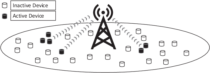
We consider the uplink of a single-cell wireless network consisting of one BS and $K$ MTC devices, as shown in Fig. 1. Let $\mathcal{K}\triangleq\{1,2,...,K\}$ denote the set of $K$ devices. Consider a discrete-time system with time being slotted. In practical MTC, adjacent devices may be triggered by the same event or dependent events. Thus, we assume that within each time slot, the devices activate according to a general $K$-dimensional binary distribution. It is worth noting that in most previous work [2, 3, 4, 5, 6, 7, 8, 9], correlation of device activities is not considered, i.e., devices are assumed to activate independently. Let $x_{k}\in\{0,1\}$ denote the activity state of device $k$, where $x_{k}=1$ if device $k$ is active, and $x_{k}=0$ otherwise. Let ${\bf x}\triangleq[x_{1},x_{2},...,x_{K}]^{T}$ denote the activity states of all $K$ devices. The device activity distribution is denoted by ${\bf p}\triangleq(p_{\bf x})_{{\bf x}\in\mathcal{X}}$, where $p_{\bf x}$ represents the probability of the activity states of the $K$ devices being $\bf x$ and $\mathcal{X}\triangleq\{0,1\}^{K}$. Note that

In practice, $p_{\bf 0}<1$.

In a slot, each active device tries to access the BS. Congestion may occur when a massive number of active devices require to access the BS at the same time. We adopt access barring scheme for access control [2]. In particular, at the beginning of each time slot, each active device independently attempts to access the BS with probability $\epsilon$, where

Here, $\epsilon$ is referred to as the access barring factor and will be optimized later. That is, the access barring scheme is parameterized by the access barring factor $\epsilon$.

We adopt the random access procedure which consists of four stages, i.e., preamble transmission, random access response, scheduled transmission and contention resolution [1]. We focus only on the first stage, where the success of access is mainly determined [2, 3, 5, 6, 7, 8, 9]. Consider $N$ orthogonal preambles, the set of which is denoted by $\mathcal{N}\triangleq\{1,2,...,N\}$. Specifically, at the first stage, each device that attempts to access the BS independently selects a preamble out of the $N$ preambles to transmit. The probability that device $k$ selects preamble $n$ is denoted by $a_{k,n}$, which satisfies

Let ${\bf a}_{k}\triangleq(a_{k,n})_{n\in\mathcal{N}}$ denote the preamble selection distribution of device $k$. Let ${\bf A}\triangleq({a}_{k,n})_{k\in\mathcal{K},n\in\mathcal{N}}$ denote the distributions of the $K$ devices. The $k$-th row of $\bf A$ is ${\bf a}_{k}$. Note that for all $k\in\mathcal{K}$, the random preamble transmission parameterized by ${\bf a}_{k}$ reduces to the preamble transmission in the standard random access procedure [1] when $a_{k,n}=\frac{1}{N}$, $n\in\mathcal{N}$. Furthermore, note that for all $k\in\mathcal{K}$, the considered preamble selection is in general random, and becomes deterministic when $a_{k,n}\in\{0,1\},n\in\mathcal{N}$. We allow ${\bf a}_{k}$, $k\in\mathcal{K}$ to be arbitrary distributions to more effectively avoid collision caused by the correlation of device activities.

If a preamble is selected by a single device, this device successfully accesses the BS [5]. Then, the average number of devices that successfully access the BS at activity states $\bf x$ in a slot is given by [10]

where the average is taken over random access control and random preamble selections.

In this paper, to obtain first-order design insights, we assume that the device activity distribution has been estimated by some learning methods as in [10], and the estimation error is negligible. That is, the exact value of $\bf p$ is known. We adopt the average throughput [10]

as the performance metric, where $T({\bf A},{\epsilon},{\bf x})$ is given by (11).

In this section, we formulate the average throughput maximization problem which is a challenging non-convex problem, and characterize an optimality property of the optimal point. Specifically, we optimize the preamble selection distributions $\bf A$ and the access barring factor $\epsilon$ to maximize the average throughput $\bar{T}({\bf A},{\epsilon},\bf p)$ in (5) subject to the constraints on $({\bf A},\epsilon)$ in (2a), (2b), (10a) and (10b).

Note that the objective function $\bar{T}(\mathbf{A},\epsilon,\bf p)$ of Problem 1, which is the exact average throughput, reflects the correlation of the activities of all devices. In contrast, [10] optimizes two approximate functions of the average throughput which only reflect the correlation of the activities of every two devices. Intuitively, solving Problem 1 will provide random access design that is more applicable to IoT applications with correlated device activities. The objective function $\bar{T}(\mathbf{A},\epsilon,\bf p)$ is nonconcave in $({\bf A},\epsilon)$, and the constraints in (2a), (2b), (10a) and (10b) are linear. Thus, Problem 1 is nonconvex. In general, a globally optimal point of a nonconvex problem cannot be obtained effectively and efficiently. Obtaining a stationary point is the classic goal for dealing with a nonconvex problem. However, we can characterize an optimality property of a globally optimal point of Problem 1.

Based on the BCD method, we propose an iterative algorithm to obtain a stationary point of Problem 1. Specifically, we divide the variables $\left({\bf A},\epsilon\right)$ into $K+1$ blocks, i.e., ${\bf a}_{k},\ k\in\mathcal{K}$ and $\epsilon$. In each iteration of the proposed algorithm, all $K+1$ blocks are sequentially updated once. At each step of one iteration, we maximize $\bar{T}(\mathbf{A},\epsilon,\bf p)$ with respect to one of the block. For ease of illustration, in the following, we also write $\bar{T}(\mathbf{A},\epsilon,\bf p)$ as $\bar{T}({\bf a}_{k},{\bf a}_{-k},\epsilon,\bf p)$, where ${\bf a}_{-k}\triangleq({\bf a}_{j})_{j\in{\mathcal{K}},j\neq k}$. Given ${\bf a}_{-k}$ and $\epsilon$ obtained in the previous step, the block coordinate optimization with respect to ${\bf a}_{k}$ is given by

Given $\bf A$ obtained in the previous step, the block coordinate optimization with respect to $\epsilon$ is given by

Each problem in (6) is a linear program (LP) with $N$ variables and $N+1$ constraints. The problem in (7) is a polynomial programming with a single variable and two constraints. Next, we obtain optimal points of the problems in (6) and (7).

Let $Q_{k,n}({\bf a}_{-k},\epsilon,{\bf p}),k\in\mathcal{K},n\in\mathcal{N}$ and $q({\bf A},\epsilon,{\bf p})$ denote the partial derivatives of $\bar{T}({\bf a},\epsilon,\bf p)$ with respect to $a_{k,n},k\in\mathcal{K},n\in\mathcal{N}$ and $\epsilon$, respectively, as shown in (8) and (9) at the top of this page. Denote $\mathcal{B}({\bf A},{\bf p})\triangleq\{z\in[0,1]:q({\bf A},z,{\bf p})=0\}$ as the set of roots of equation $q({\bf A},z,{\bf p})=0$ that lie in interval $[0,1]$. Based on structural properties of the block coordinate optimization problems in (6) and (7), we can obtain their optimal points.

From the complexity analysis for obtaining a stationary point of Problem 1, we know that Algorithm 1 is computationally expansive when $K$ or $N$ is large. In this section, we develop another iterative algorithm to obtain a low-complexity solution of Problem 1, which is applicable for large $K$ or $N$. Later, in Section VI, we shall show that such low-complexity algorithm achieves competitive average throughput compared with Algorithm 1, although it has much lower computational complexity than Algorithm 1.

First, we approximate the complicated function $\bar{T}(\mathbf{A},\epsilon,{\bf p})$, which has $N2^{K}$ terms, with a simpler function, which has $1+\frac{K(K-1)}{2}$ terms. Motivated by the approximations of $\bar{T}(\mathbf{A},\epsilon,{\bf p})$ in [10], we consider approximate function parameterized by $\lambda\in\mathbb{R}$ as shown in (12) at the top of this page. Note that $\sum\nolimits_{{\bf x}\in\mathcal{X}}p_{\bf x}x_{k}$ and $\sum\nolimits_{{\bf x}\in\mathcal{X}}p_{\bf x}x_{k}x_{l}$ ($k<l$) represent the probability of device $k$ being active and probability of devices $k$ and $l$ being active, respectively. Though $\sum\nolimits_{{\bf x}\in\mathcal{X}}p_{\bf x}x_{k}$ and $\sum\nolimits_{{\bf x}\in\mathcal{X}}p_{\bf x}x_{k}x_{l}$ contain $2^{K}$ terms and are hard to compute, in practice, they can be easily approximated from empirical activity states. By comparing (12) with (5), we can see that $\tilde{T}_{\lambda}(\mathbf{A},\epsilon,{\bf p})$ captures the activity probabilities of a single device and every two devices. For all $({\bf A},\epsilon)$ satisfying (2a), (2b), (10a), (10b) and all $\bf p$ satisfying (1a) and (1b), we can obtain an upper bound on the approximation error:

The upper bound in (13) is minimized at $\lambda=\frac{1}{2}$, which can be easily shown. Thus, we approximate $\bar{T}(\mathbf{A},\epsilon,{\bf p})$ with $\tilde{T}_{\frac{1}{2}}\left(\mathbf{A},\epsilon,{\bf p}\right)$, and consider the following approximate problem of Problem 1.

Analogously, using the BCD method, we propose a computationally efficient iterative algorithm to obtain a stationary point of Problem 2, which has more performance guarantee than the heuristic method in [10]. Specifically, variables $\left({\bf A},\epsilon\right)$ are divided into $K+1$ blocks, i.e., ${\bf a}_{k},\ k\in\mathcal{K}$ and $\epsilon$. For ease of illustration, in the following, we also write $\tilde{T}_{\frac{1}{2}}(\mathbf{A},\epsilon,\bf p)$ as $\tilde{T}_{\frac{1}{2}}({\bf a}_{k},{\bf a}_{-k},\epsilon,\bf p)$. Given ${\bf a}_{-k}$ and $\epsilon$ obtained in the previous step, the block coordinate optimization with respect to ${\bf a}_{k}$ is given by

Given $\bf A$ obtained in the previous step, the block coordinate optimization with respect to $\epsilon$ is given by

Each problem in (14) is an LP with $N$ variables and $N+1$ constraints, and the problem in (15) is a quadratic program (QP) with a single variable and two constraints. It is clear that the convex problems in (14) and (15) are much simpler than those in (6) and (7), respectively.

Based on structural properties of the block coordinate optimization problems in (14) and (15), we can obtain their optimal points.

In this section, we evaluate the performance of the proposed solutions via numerical results. We consider three baseline schemes, namely BL-MMPC, BL-MSPC and BL-LTE. In BL-MMPC and BL-MSPC, ${\bf a}_{k}$, $k\in\mathcal{K}$ are obtained by the MMPC and MSPC allocation algorithms in [10], respectively, and $\epsilon=1$. In BL-LTE, we set $a_{k,n}=\frac{1}{N},\ k\in\mathcal{K},n\in\mathcal{N}$ according to the standard random access procedure of LTE networks [1], and set $\epsilon=\min\left(1,\frac{N}{\bar{K}}\right)$ according to the optimal access control [2], where $\bar{K}$ denotes the average number of active devices. Note that BL-MMPC and BL-MSPC make use of the correlation of the activities of every two devices; BL-LTE does not utilize any information on correlation of device activities. In the simulation, we adopt the group device activity model. Specifically, $K$ devices are divided into $G$ groups each of size $\frac{K}{G}$ (assuming $K$ is divisible by $G$), the activity states of devices in different groups are independent, and the activity states of devices in a group are the same. The probability that a group is active, i.e., all devices in this group are active, is $p_{a}$. Then, $\bf x$ and $p_{\bf x},{\bf x}\in\mathcal{X}$ can be easily determined.

First, we compare the average throughput of the proposed solutions and three baseline schemes, at small numbers of devices and preambles. Fig. 2 illustrates the average throughput versus the number of devices $K$ and the number of preambles $N$. From Fig. 2, we make the following observations. The proposed stationary point significantly outperforms BL-MMPC and BL-MSPC, as the stationary point relies on $p_{\bf x}$, ${\bf x}\in\mathcal{X}$, which capture the correlation of the activities of all devices; BL-MMPC and BL-MSPC outperform BL-LTE, as BL-MMPC and BL-MSPC both make use of the correlation of the activities of every two devices. The proposed low-complexity solution outperforms BL-MMPC and BL-MSPC, as it relies on a more accurate approximation of the average throughput and is obtained by a more effective algorithm; it is worth noting that the gap between the average throughput of the stationary point and the low-complexity solution is small, which shows that exploiting the correlation of the activities of every two devices in a rigorous way already achieves a significant gain. Furthermore, from Fig. 2 (a), we can see that the average throughput of each scheme increases with $K$, due to the increase of traffic load. From Fig. 2 (b), we can see that the average throughput of each scheme increases with $N$, due to the increase of communications resource.

Next, we compare the average throughputs of the proposed solutions and three baseline schemes, at large numbers of devices and preambles. Fig. 3 illustrates the average throughput versus the number of devices $K$ and the number of preambles $N$. From Fig. 3, we also observe that the low-complexity solution significantly outperforms BL-MMPC, BL-MSPC and BL-LTE; the results at large $K$ and $N$ shown in Fig. 3 are similar to those at small $K$ and $N$ shown in Fig. 2.

In this paper, we investigated the joint optimization of preamble selection and access barring for correlated device activities which exist in most IoT applications and is important for 6G. We optimized the preamble selection distribution and the access barring factor to maximize the average throughput of the devices. We characterized an optimality property and obtained a stationary point and a low-complexity solution. We numerically showed that the two proposed solutions achieve significant gains over existing schemes and have a small gap in average throughput. The numerical results demonstrate the significance of exploiting the correlation of activities of every two devices in a rigorous way. Both the theoretical and numerical results offer important design insights for MTC.

References

- [1] 3GPP, “Evolved universal terrestrial radio access (E-UTRA); medium access control (MAC) protocol specification,” TS 36.321, Apr, 2015.
- [2] S. Duan, V. Shah-Mansouri, Z. Wang, and V. W. S. Wong, “D-ACB: Adaptive congestion control algorithm for bursty M2M traffic in LTE networks,” IEEE Trans. Veh. Technol., vol. 65, no. 12, pp. 9847–9861, Dec. 2016.
- [3] Z. Wang and V. W. S. Wong, “Optimal access class barring for stationary machine type communication devices with timing advance information,” IEEE Trans. Wireless Commun., vol. 14, no. 10, pp. 5374–5387, Oct. 2015.
- [4] M. Vilgelm, S. Rueda Liares, and W. Kellerer, “On the resource consumption of M2M random access: Efficiency and pareto optimality,” IEEE Wireless Commun. Lett., vol. 8, no. 3, pp. 709–712, Jun. 2019.
- [5] W. Zhan and L. Dai, “Massive random access of machine-to-machine communications in LTE networks: Modeling and throughput optimization,” IEEE Trans. Wireless Commun., vol. 17, no. 4, pp. 2771–2785, Apr. 2018.
- [6] C. Di, B. Zhang, Q. Liang, S. Li, and Y. Guo, “Learning automata-based access class barring scheme for massive random access in machine-to-machine communications,” IEEE Internet Things J., vol. 6, no. 4, pp. 6007–6017, Aug. 2019.
- [7] H. Jin, W. T. Toor, B. C. Jung, and J. Seo, “Recursive pseudo-bayesian access class barring for M2M communications in LTE systems,” IEEE Trans. Veh. Technol., vol. 66, no. 9, pp. 8595–8599, Sep. 2017.
- [8] C. Oh, D. Hwang, and T. Lee, “Joint access control and resource allocation for concurrent and massive access of M2M devices,” IEEE Trans. Wireless Commun., vol. 14, no. 8, pp. 4182–4192, Aug. 2015.
- [9] J. Choi, “On the adaptive determination of the number of preambles in RACH for MTC,” IEEE Wireless Commun. Lett., vol. 20, no. 7, pp. 1385–1388, Jul. 2016.
- [10] A. E. Kalor, O. A. Hanna, and P. Popovski, “Random access schemes in wireless systems with correlated user activity,” in Proc. IEEE SPAWC, Jun. 2018, pp. 1–5.
- [11] S. Boyd, S. P. Boyd, and L. Vandenberghe, Convex optimization. Cambridge university press, 2004.
- [12] D. P. Bertsekas, Nonlinear progranmming. Athena scientific Belmont, MA, 1998.