跳到论文正文
W Papers独立论文阅读器 arXiv:2104.05886 论文正文 计算阅读时间 · 0%
引用这篇论文根据当前论文元数据生成,正式投稿前建议核对。


License: arXiv.org perpetual non-exclusive license
arXiv:2104.05886v3 [stat.CO] 05 Jul 2023

∎

The computational asymptotics of Gaussian variational inference and the Laplace approximation

Zuheng Xu Affiliation: Department of Statistics, The University of British Columbia, Vancouver, Canada E-mail: zuheng.xu@stat.ubc.ca    Trevor Campbell Affiliation: Department of Statistics, The University of British Columbia, Vancouver, Canada E-mail: trevor@stat.ubc.ca
Received: date / Accepted: date
Abstract

Gaussian variational inference and the Laplace approximation are popular alternatives to Markov chain Monte Carlo that formulate Bayesian posterior inference as an optimization problem, enabling the use of simple and scalable stochastic optimization algorithms. However, a key limitation of both methods is that the solution to the optimization problem is typically not tractable to compute; even in simple settings the problem is nonconvex. Thus, recently developed statistical guarantees—which all involve the (data) asymptotic properties of the global optimum—are not reliably obtained in practice. In this work, we provide two major contributions: a theoretical analysis of the asymptotic convexity properties of variational inference with a Gaussian family and the maximum a posteriori (MAP) problem required by the Laplace approximation; and two algorithms—consistent Laplace approximation (CLA) and consistent stochastic variational inference (CSVI)—that exploit these properties to find the optimal approximation in the asymptotic regime. Both CLA and CSVI involve a tractable initialization procedure that finds the local basin of the optimum, and CSVI further includes a scaled gradient descent algorithm that provably stays locally confined to that basin. Experiments on nonconvex synthetic and real-data examples show that compared with standard variational and Laplace approximations, both CSVI and CLA improve the likelihood of obtaining the global optimum of their respective optimization problems.

Keywords: 
Bayesian statistics variational inference Laplace approximation computational asymptotics Bernstein-von Mises

1 Introduction

Bayesian statistical models are powerful tools for learning from data, with the ability to encode complex hierarchical dependence and domain expertise, as well as coherently quantify uncertainty in latent parameters. For many modern Bayesian models, exact computation of the posterior is intractable (Blei et al. 2017, Section 2.1) and statisticians must resort to approximate inference algorithms. Currently, the most popular type of Bayesian inference algorithm in statistics is Markov Chain Monte Carlo (MCMC) (Hastings 1970; Gelfand and Smith 1990; Robert and Casella 2013), which provides approximate samples from the posterior distribution and is supported by a comprehensive literature of theoretical guarantees (Roberts and Rosenthal 2004; Meyn and Tweedie 2012). An alternative—variational inference (Jordan et al. 1998; Wainwright and Jordan 2008; Blei et al. 2017)—approximates the intractable posterior with a distribution chosen from a pre-specified family, e.g., the family of Gaussian distributions parametrized by mean and covariance. The approximating distribution is chosen by minimizing a discrepancy (e.g., Kullback-Leibler (KL) (Murphy 2012, Section 2.8) or Rényi divergence (Van Erven and Harremos 2014)) to the posterior distribution over the family. Another alternative—the Laplace approximation (Shun and McCullagh 1995; Hall et al. 2011)—involves first finding the maximum of the posterior density, and then fitting a Gaussian using a second-order Taylor expansion. Both methods convert Bayesian inference into an optimization problem, enabling the use of simple, scalable stochastic optimization algorithms (Robbins and Monro 1951; Bottou 2004) that require only a subsample of the data at each iteration and avoid computation on the entire dataset.

But despite their scalability, both variational inference and the Laplace approximation have key limitations. First, one is forced to use an approximation of the posterior from a preselected parametric family of distributions. In particular, the Laplace approximation involves the family of Gaussians, while in variational inference the choice of family is left to the practitioner. In either case, it is in general difficult to know how limited the family is before actually optimizing; and not only that, it is also often difficult to estimate the approximation error once the optimization is complete (Huggins et al. 2020). For example, if one uses a mean-field Gaussian family with a diagonal covariance, the resulting posterior approximation will typically underestimate posterior variances and cannot capture its covariances (Murphy 2012, Section 21.2.2), two quantities of particular interest to statisticians. The second key limitation is that even if the Laplace approximation or optimal variational approximation are known to have low error, the optimization problems required by both methods are typically nonconvex, and the global optimum cannot be found reliably.

The key to addressing the first limitation is to understand the optimal approximation error within the chosen family. Aside from nonparametric mixtures (Guo et al. 2016; Miller et al. 2017; Locatello et al. 2018; Campbell and Li 2019)—which can be designed to achieve arbitrary approximation quality—available results in the finite-data setting are quite limited. For example, Han and Yang 2019 provides a non-asymptotic analysis of optimal mean-field variational approximations, but extending these results to more general distribution families is not straightforward. On the other hand, multiple threads of research have explored the statistical properties of parametric posterior approximations in the data-asymptotic regime by taking advantage of the limiting behavior of the Bayesian posterior. The Laplace approximation is well studied in statistical literature in this regard (Shun and McCullagh 1995; Hall et al. 2011; Miller 2021; Bassett and Deride 2019; Barber et al. 2016), while research on variational inference is ongoing. Wang and Blei 2019 exploits the asymptotic normality of the posterior distribution in a parametric Bayesian setting to show that the variational KL minimizer asymptotically converges to the KL minimizer to the limiting normal posterior distribution. Alquier and Ridgway 2020 analyze the rate of convergence of the variational approximation to a fractional posterior—a posterior with a tempered likelihood—in a high dimensional setting where the posterior itself may not have the ideal asymptotic behavior. Zhang and Gao 2020 studies the contraction rate of the variational distribution for non-parametric Bayesian inference and provides general conditions on the Bayesian model that characterizes the rate. Yang et al. 2020 and Jaiswal et al. 2019 build a framework for analyzing the statistical properties of α\alpha-Rényi variational inference, and provide sufficient conditions that guarantee an optimal convergence rate of the obtained point estimate. But while the literature has built a comprehensive understanding of the asymptotic guarantees of both the Laplace and optimal variational approximations, the nonconvexity of the optimization problems involved makes these guarantees difficult to obtain reliably in practice. In fact, 12 of the present work demonstrates that both the Laplace approximation and Gaussian variational inference involve nonconvex optimization, even in simple cases with ideal asymptotic posterior behaviour.

In this work, we address the nonconvexity of Gaussian variational inference and the maximum a posteriori (MAP) problem in the data-asymptotic regime when the posterior distribution admits asymptotic normality. Rather than focusing on the statistical properties of the optimum, we investigate the asymptotic properties of the optimization problems themselves (Section 4), and use these to design procedures (Section 3) which involve only tractable optimization and hence make theoretical results regarding global optima applicable. In particular, we develop consistent stochastic variational inference (CSVI) and consistent Laplace approximation (CLA), two algorithms for Gaussian posterior approximation. CSVI is guaranteed to find the optimal variational approximation, and CLA the maximum a posteriori (MAP), with probability that converges to 11 in the limit of observed data. The first key innovation in both CSVI and CLA is that we initialize the optimization at the mode of a smoothed posterior—the posterior distribution convolved with Gaussian noise. We prove that, with enough data, the smoothed MAP falls in a local region in which the optimization problem is locally convex and contains the global optimum, and that finding the smoothed MAP is a convex optimization problem and hence tractable (Section 4.3). The second innovation, which pertains only to CSVI, is a gradient scaling during stochastic optimization (Section 3.3) that ensures that the optimization remains inside the aforementioned local region and converges to the global optimum. Experiments on synthetic examples in Section 5 show that CSVI and CLA provide numerically stable and asymptotically consistent posterior approximations.

2 Variational and Laplace posterior approximations

In the setting of Bayesian inference considered in this paper, we are given a sequence of posterior distributions Πn\Pi_{n}, n∈ℕn\in\mathbb{N} each with full support on ℝd\mathbb{R}^{d}. The index nn represents the amount of observed data; denote Π0\Pi_{0} to be the prior. We also assume that each posterior Πn\Pi_{n} has density πn\pi_{n} with respect to the Lebesgue measure.

2.1 Gaussian variational inference

Gaussian variational inference aims to find a Gaussian approximation to the posterior distribution by solving the optimization problem

arg​minμ∈ℝd,Σ∈ℝd×dDKL(𝒩(μ,Σ)||Πn)s.t.Σ≻0,\displaystyle\begin{aligned} \operatornamewithlimits{arg\,min}_{\mu\in\mathbb{R}^{d},\Sigma\in\mathbb{R}^{d\times d}}\quad&\mathrm{D_{KL}}\left(\mathcal{N}(\mu,\Sigma)||\Pi_{n}\right)\quad\text{s.t.}\quad\Sigma\succ 0,\end{aligned} (2)

where the Kullback-Leibler divergence (Murphy 2012, Section 2.8) is defined as

DKL(Q||P):=∫logd​Qd​PdQ\displaystyle\mathrm{D_{KL}}\left(Q||P\right):=\int\log\frac{\mathrm{d}Q}{\mathrm{d}P}\mathrm{d}Q (3)

for any pair of probability distributions P,QP,Q such that Q≪PQ\ll P, and d​Qd​P\frac{\mathrm{d}Q}{\mathrm{d}P} is the Radon-Nikodym derivative of QQ with respect to PP (Folland 1999, Section 3.2). We use the standard reparametrization of Σ\Sigma using the Cholesky factorization Σ=n−1​L​LT\Sigma=n^{-1}LL^{T} to arrive at the common formulation of Gaussian variational inference (Kucukelbir et al. 2017) that is the focus of the present work:

μn⋆,Ln⋆=arg​minμ∈ℝd,L∈ℝd×d−n−1​log​detL+Fn​(μ,L)s.t.L​ lower triangular with positive diagonal,\displaystyle\begin{aligned} \mu_{n}^{\star},L_{n}^{\star}&=\operatornamewithlimits{arg\,min}_{\mu\in\mathbb{R}^{d},L\in\mathbb{R}^{d\times d}}\!-n^{-1}\log\det L+F_{n}(\mu,L)\\ &\text{s.t.}\quad L\text{ lower triangular with positive diagonal},\end{aligned} (4)

where

fn​(x)\displaystyle f_{n}(x) :=−n−1​log⁡πn​(x)\displaystyle:=-n^{-1}\log\pi_{n}(x) (5)
Fn​(μ,L)\displaystyle F_{n}(\mu,L) :=𝔼[fn(μ+n−1/2LZ)],Z∼𝒩(0,I).\displaystyle:=\mathbb{E}\left[f_{n}(\mu+n^{-1/2}LZ)\right],\quad Z\sim\mathcal{N}(0,I). (6)

Denote the optimal Gaussian distribution

𝒩VI,n:=𝒩⁡(μn⋆,n−1​Ln⋆​Ln⋆T).\displaystyle\mathcal{N}_{\text{VI,n}}:=\mathcal{N}(\mu^{\star}_{n},n^{-1}L_{n}^{\star}L_{n}^{\star T}). (7)

Intuitively, this optimization problem encodes a tradeoff between maximizing the expected posterior density under the variational approximation—which tries to make LL small and move μ\mu close to the maximum point of πn\pi_{n}—and maximizing the entropy of the variational approximation—which prevents LL from becoming too small. It crucially does not depend on the (typically unknown) normalization of πn\pi_{n}, which appears as an additive constant in Eq. 4; it is common to drop this constant and instead equivalently maximize the expectation lower bound (ELBO) (Blei et al. 2017). Note that there are a number of unconstrained parametrizations of the covariance matrix variable Σ\Sigma (Pinheiro and Bates 1996). We select the (unique) positive-diagonal Cholesky factor LL as it makes the optimization problem Eq. 4 more amenable to both theoretical analysis and computational optimization.

One typically attempts to solve Eq. 4 using an iterative local descent optimization algorithm. As the expectation is intractable in most scenarios, this involves stochastic optimization (Hoffman et al. 2013; Ranganath 2014; Kingma and Welling 2014; Kucukelbir et al. 2017). In particular, assuming one can interchange expectation and differentiation (see Section 4.1 for details), the quantities

∇^μ,n​(μ,L,Z):=∇fn(μ+n−1/2LZ)∇^L,n​(μ,L,Z):=−n−1​(diag⁡L)−1+n−1/2tril∇fn(μ+n−1/2LZ)ZT,\displaystyle\begin{aligned} \hat{\nabla}_{\mu,n}(\mu,L,Z)\!&:=\!\nabla f_{n}(\mu+n^{-1/2}LZ)\\ \hat{\nabla}_{L,n}(\mu,L,Z)\!&:=\!-n^{-1}(\operatorname{diag}L)^{-1}\\ &\quad+n^{-1/2}\mathrm{tril}\,\nabla f_{n}(\mu+n^{-1/2}LZ)Z^{T},\end{aligned} (8)

are unbiased estimates of the μ\mu- and LL-gradients of the objective in Eq. 4 given Z∼𝒩⁡(0,I)Z\sim\mathcal{N}(0,I), where the functions diag:ℝd×d→ℝd×d\operatorname{diag}:\mathbb{R}^{d\times d}\to\mathbb{R}^{d\times d} and tril:ℝd×d→ℝd×d\mathrm{tril}\,:\mathbb{R}^{d\times d}\to\mathbb{R}^{d\times d} set the off-diagonal and upper triangular elements of their arguments to 0, respectively. These unbiased gradient estimates may be used in a wide variety of stochastic optimization algorithms (Robbins and Monro 1951; Bottou 2004) applied to Eq. 4. In this paper, we will focus on projected stochastic gradient descent (SGD) (Bubeck 2015, Section 3.) due to its simplicity; we expect that the mathematical theory in this work extends to other related methods. In general, Gaussian variational inference is a nonconvex optimization problem and standard iterative methods such as SGD are not guaranteed to produce a sequence of iterates that converge to μn⋆,Ln⋆\mu_{n}^{\star},L_{n}^{\star}.

2.2 Laplace approximation

The Laplace approximation (Bishop and Nasrabadi 2006, Section 4.4) constructs a Gaussian approximation to the posterior centered at the maximum a posteriori (MAP) point θn⋆\theta_{n}^{\star}, and with covariance based on a second-order Taylor expansion of log⁡πn\log\pi_{n} at the MAP, i.e.,

𝒩Lap,n\displaystyle\mathcal{N}_{\text{Lap},n} :=𝒩⁡(θn⋆,ΣLap,n)\displaystyle:=\mathcal{N}(\theta^{\star}_{n},\Sigma_{\text{Lap},n}) (9)
θn⋆\displaystyle\theta^{\star}_{n} =arg​minθ∈ℝd⁡fn​(θ)\displaystyle=\operatornamewithlimits{arg\,min}_{\theta\in\mathbb{R}^{d}}f_{n}(\theta) (10)
ΣLap,n\displaystyle\Sigma_{\text{Lap},n} :=(−∇2​log​πn​(θn⋆))−1.\displaystyle:=\left(-\nabla^{2}\log\pi_{n}(\theta^{\star}_{n})\right)^{-1}. (11)

Under certain regularity conditions, the total variation error of the Laplace approximation diminishes as the number of samples increases (Kass 1990; Miller 2021; Schillings et al. 2020); we present the precise statement in 5. However, since log⁡πn\log\pi_{n} is typically not concave, obtaining the MAP point—and hence computing the Laplace approximation—is generally intractable.

3 Consistent variational and Laplace approximations

In this section, we provide two methods—Consistent Stochastic Variational Inference (CSVI) and Consistent Laplace (CLA)—that asymptotically solve the Gaussian variational inference and MAP problems in Eqs. 4 and 10 in the sense that the probability that the iterates converge to the global optimum converges to 11 in the asymptotic limit of observed data (see 1). The development of the algorithms and results in this section depend heavily on asymptotic convexity and smoothness analysis later in Section 4. While the interested reader can refer to that section for a precise treatment, the key intuitive points in the development are that, very informally: (1) fnf_{n} is generally nonconvex, even asymptotically in well-behaved models, and this renders both the MAP and variational inference problems nonconvex; however, (2) both optimization problems are asymptotically locally strongly convex around a fixed location θ0\theta_{0}, and μn⋆\mu^{\star}_{n} and θn⋆\theta^{\star}_{n} both converge to θ0\theta_{0}; and (3) the posterior density smoothed by a Gaussian kernel is asymptotically log concave, and the smoothed MAP θ^n⋆\hat{\theta}^{\star}_{n} also converges to θ0\theta_{0}. Therefore in CSVI and CLA, we first use the smoothed posterior MAP θ^n⋆\hat{\theta}^{\star}_{n} as a tractable initialization near the global optimum, and carefully scale gradient steps while optimizing so as to remain in the local basin around the optimum. In the remainder of this section, we provide the details of the smoothed MAP optimization, CSVI, and CLA; theoretical details are deferred to Section 4.

Similar two-stage designs involving initialization followed by local optimization have been employed for nonconvex problems in statistics, e.g., Balakrishnan et al. 2017. However, this work assumes the existence of the initialization—which generally requires intractable nonconvex optimization itself—and requires a model-specific theoretical analysis to tune the local optimization method. In contrast, our work provides practical, model-agnostic, and asymptotically tractable optimization methods.

Refer to caption
Refer to caption
Figure 1: Top: A synthetic Bayesian model with posterior density for increasing dataset sizes (n=10,100,1000,10000n=10,100,1000,10000). The posterior density displayed in the figure are normalized, fixing the maximum at 100100. The details of this synthetic model and experimental setup can be found in Section A.1. Bottom: The smoothed Bayesian posterior densities corresponding to the top row. Black curves show the smoothed posterior (with smoothing constant of αn=10​n−0.3\alpha_{n}=10n^{-0.3}), the blue histogram shows the counts (over 100 trials) of the output of the smoothed MAP initialization, and the red dots denote the last iteration of the smoothed MAP optimization.

3.1 Smoothed MAP initialization

Given the nthn^{\text{th}} posterior distribution Πn\Pi_{n}, we define the smoothed posterior Π^n\hat{\Pi}_{n} with smoothing variance αn\alpha_{n} to be the θ\theta-marginal of the generative process

W∼Πn,θ∼𝒩⁡(W,αn​I).\displaystyle W\sim\Pi_{n},\quad\theta\sim\mathcal{N}(W,\alpha_{n}I). (12)

The probability density function π^n\hat{\pi}_{n} of Π^n\hat{\Pi}_{n} is given by the convolution of πn\pi_{n} with a multivariate normal density,

π^n​(θ)=\displaystyle\hat{\pi}_{n}(\theta)= 𝔼⁡[1(2​π)d/2​αnd/2​exp⁡(−12​αn​‖θ−W‖2)].\displaystyle\mathbb{E}\left[\frac{1}{(2\pi)^{d/2}\alpha_{n}^{d/2}}\exp\left(-\frac{1}{2\alpha_{n}}\|\theta-W\|^{2}\right)\right]. (13)

Given these definitions, the smoothed MAP problem is the MAP inference problem for the smoothed posterior distribution, i.e.,

θ^n⋆=\displaystyle\hat{\theta}^{\star}_{n}= arg​minθ∈ℝd−log⁡𝔼⁡[exp⁡(−12​αn​‖θ−W‖2)].\displaystyle\operatornamewithlimits{arg\,min}_{\theta\in\mathbb{R}^{d}}\,\,-\log\mathbb{E}\left[\exp\left(-\frac{1}{2\alpha_{n}}\|\theta-W\|^{2}\right)\right]. (14)

Gaussian smoothing is commonly used in image and signal processing (Forsyth and Ponce 2002; Nixon and Aguado 2012; Haddad and Akansu 1991; Lindeberg 1990), and has previously been applied to reduce the presence of spurious local optima in nonconvex optimization problems, making them easier to solve with local gradient-based methods (Addis et al. 2005; Mobahi 2013). This effect is demonstrated in Fig. 1, where we construct a synthetic Bayesian model where the posterior is asymptotically normal but has multiple modes even given a large sample size. The details of this synthetic model and the setting of the experiment can be found in Section A.1. The variance αn\alpha_{n} controls the degree of smoothing; larger values create a smoother density π^n\hat{\pi}_{n}, at the cost of making π^n\hat{\pi}_{n} a poorer approximation of the original function πn\pi_{n}. Fig. 2 demonstrates how increasing αn\alpha_{n} increases the smoothing effect, resulting in fewer and flatter local optima in the objective. In practice with a fixed finite data set, one needs to tune the smoothing constant αn\alpha_{n}. However, we show later in 7 that if αn\alpha_{n} satisfies n​αn3→∞n\alpha_{n}^{3}\to\infty, then eventually Eq. 14 becomes a convex problem, and θ^n⋆\hat{\theta}^{\star}_{n} converges in probability to the original posterior mode θn⋆\theta^{\star}_{n}.

Refer to caption
Figure 2: Plots of the smoothed posterior density π^n\hat{\pi}_{n} with increasing smoothing variance α\alpha. Note that α=0\alpha=0 denotes the original posterior.

We use SGD to solve the smoothed MAP problem. By change of variables and reparametrization, the gradient of the smoothed MAP objective function in Eq. 14 is

∇(−log⁡π^n​(θ))=\displaystyle\nabla(-\log\hat{\pi}_{n}(\theta))= αn−1/2𝔼⁡[W​πn​(θ−αn1/2​W)]𝔼⁡[πn​(θ−αn1/2​W)],\displaystyle\,\alpha_{n}^{-1/2}\frac{\mathbb{E}\left[W\pi_{n}\left(\theta-\alpha_{n}^{1/2}W\right)\right]}{\mathbb{E}\left[\pi_{n}\left(\theta-\alpha_{n}^{1/2}W\right)\right]}, (15)

where W∼𝒩⁡(0,I)W\sim\mathcal{N}\left(0,I\right). Note that the unknown normalization constant in πn\pi_{n} cancels in the numerator and denominator. We obtain stochastic estimates of the gradient using a Monte Carlo approximation of the numerator and denominator using the same samples, i.e., self-normalized importance sampling (Robert and Casella 2013, p. 95). It is known that the variance of this gradient estimate may be quite large or even infinite; although techniques such as truncation (Ionides 2008) and smoothing (Vehtari et al. 2015) exist to address it, we leave this issue as an open problem for future work. The resulting SGD procedure with explicit gradient estimates are shown in Algorithm 1.

Algorithm 1 Smoothed MAP optimization
procedure SmoothedMAP(πn\pi_{n}, αn\alpha_{n}, KK, SS, (γk)k∈ℕ(\gamma_{k})_{k\in\mathbb{N}})
  θ←0\theta\leftarrow 0
  for k=1,…,Kk=1,\dots,K do
   Sample (Zs)s=1S​∼i.i.d. ​𝒩​(0,I)(Z_{s})_{s=1}^{S}\overset{\textrm{\tiny{i.i.d.}{} }}{\sim}\mathcal{N}(0,I)
   g^←αn−12​(∑s=1SZs​πn​(θ−αn12​Zs))/(∑s=1Sπn​(θ−αn12​Zs))\hat{g}\!\leftarrow\alpha_{n}^{-\frac{1}{2}}\!\left(\!\sum_{s=1}^{S}\!Z_{s}\!\pi_{n}(\theta-\alpha_{n}^{\frac{1}{2}}Z_{s})\!\right)\!\Big/\!\left(\!\sum_{s=1}^{S}\pi_{n}(\theta-\alpha_{n}^{\frac{1}{2}}Z_{s})\!\right)
   θ←θ−γk​g^\theta\leftarrow\theta-\gamma_{k}\hat{g}
  end for
  return θ\theta
end procedure

3.2 Consistent Laplace approximation (CLA)

The consistent Laplace approximation (CLA) involves first initializing θ\theta to the smoothed MAP θ^n⋆\hat{\theta}^{\star}_{n} (which we estimate with Algorithm 1), and then proceeding as in the standard Laplace approximation: we use gradient descent to find the posterior mode, and then construct 𝒩Lap,n\mathcal{N}_{\text{Lap},n} per Eq. 9. The only concern is that the iterates produced by gradient descent need to stay confined to the local basin of fnf_{n} around the optimum point; we can ensure this by using a small enough step size, or by using a line-search to set the step size adaptively (Boyd and Vandenberghe 2004, Page 466; Armijo 1966; Bertsekas and Tsitsiklis 2000). We present CLA with backtracking line search in Algorithm 2.

Algorithm 2 Consistent Laplace approximation
procedure CLA(fnf_{n}, β∈(0,1)\beta\in(0,1), KK)
  θ←\theta\leftarrowSmoothedMAP (Algorithm 1)
  for k=1,…,Kk=1,\dots,K do
   t←1t\leftarrow 1
   while fn(θ−t∇fn(θ))>fn(θ)−t2∥∇fn(θ)∥2f_{n}(\theta-t\nabla f_{n}(\theta))>f_{n}(\theta)-\frac{t}{2}\|\nabla f_{n}(\theta)\|^{2} do
     t←β​tt\leftarrow\beta t
   end while
   θ←θ−t∇fn(θ)\theta\leftarrow\theta-t\nabla f_{n}(\theta)
  end for
  return θ\theta, 1n​(∇2fn​(θ))−1\frac{1}{n}\left(\nabla^{2}f_{n}(\theta)\right)^{-1}
end procedure

We provide a convergence result for CLA in 2. In particular, under mild regularity conditions on the Bayesian model, 2 shows that CLA asymptotically solves the MAP optimization problem Eq. 10, and hence enables reliable computation of the Laplace approximation. 1 clarifies what it means for an algorithm to solve an optimization problem in the data-asymptotic limit. We use the usual notation oPno_{P_{n}} and OPnO_{P_{n}} to denote stochastic order (van der Vaart 2000, Section 2.2).

Definition 1.

An iterative algorithm asymptotically solves a (random) sequence of optimization problems indexed by n∈ℕn\in\mathbb{N}, each with a single global optimum point xn⋆∈ℝdx_{n}^{\star}\in\mathbb{R}^{d}, if the sequence of iterates (xk,n)k∈ℕ(x_{k,n})_{k\in\mathbb{N}} produced by the algorithm satisfies

limn→∞ℙ⁡(‖xk,n−xn⋆‖2=oPn​(1))=1,\displaystyle\lim_{n\to\infty}\mathbb{P}\left(\|x_{k,n}-x_{n}^{\star}\|^{2}=o_{P_{n}}(1)\right)=1, (16)

where ℙ\mathbb{P} denotes the law of the sequence of optimization problems and PnP_{n} denotes the law of the iterates of the nthn^{\text{th}} optimization problem. Further, we say that it asymptotically solves the sequence of problems at a rate tkt_{k}, if

limn→∞ℙ⁡(‖xk,n−xn⋆‖2=OPn​(tk))=1,limk→∞tk=0.\displaystyle\lim_{n\to\infty}\mathbb{P}\left(\|x_{k,n}-x_{n}^{\star}\|^{2}=O_{P_{n}}(t_{k})\right)=1,\quad\lim_{k\to\infty}t_{k}=0. (17)
Theorem 2.

Suppose 1 holds. Then there exist r,ℓ>0r,\ell>0 and 0≤η<10\leq\eta<1 such that if we initialize θ\theta such that ‖θ−θ^n⋆‖≤r4​(ℓ+1)\|\theta-\hat{\theta}^{\star}_{n}\|\leq\frac{r}{4(\ell+1)}, then CLA asymptotically solves the MAP problem Eq. 10 at a rate of ηk\eta^{k}.

The constant rr in the statement of 2 intuitively represents the radius of the local convex basin around the optimum point of fnf_{n}, and ℓ\ell is the local Lipschitz smoothness constant, as defined in 9. In practice, since the constants rr and ℓ\ell are not known, one should run the smoothed MAP optimization Algorithm 1 until convergence to θ^n⋆\hat{\theta}^{\star}_{n} according to some diagnostic, e.g., a small gradient norm.

3.3 Consistent stochastic variational inference (CSVI)

Consistent stochastic variational inference (CSVI) begins by initializing L=IL=I and μ\mu to the smoothed MAP θ^n⋆\hat{\theta}^{\star}_{n} (which we estimate with Algorithm 1), and then optimizes the variational objective Eq. 4 using projected stochastic gradient descent (SGD) (Bubeck 2015, Section 3). Much like in CLA, the remaining concern is that the iterates of SGD stay within the local region around the optimum μn⋆,Ln⋆\mu^{\star}_{n},L^{\star}_{n} in which the variational objective is strongly convex. The major issue is that the regularization term −n−1logdetL-n^{-1}\log\det L in the objective of Eq. 4 is not Lipschitz smooth, which both makes theoretical guarantees on convergence difficult to obtain and in practice results in instability in LL during optimization. We address this issue by applying a novel scaling matrix to the gradient steps; in particular, define the scaled LL gradient matrix ∇~L,n​(μ,L,Z)∈ℝd×d\tilde{\nabla}_{L,n}(\mu,L,Z)\in\mathbb{R}^{d\times d} via

[∇~L,n​(μ,L,Z)]i​j\displaystyle\left[\tilde{\nabla}_{L,n}(\mu,L,Z)\right]_{ij} (18)
={[∇^L,n​(μ,L,Z)]i​jj≠i11+(n​Li​i)−1​[∇^L,n​(μ,L,Z)]i​ij=i,Li​i>0−1j=i,Li​i=0.\displaystyle=\left\{\begin{array}[]{ll}\left[\hat{\nabla}_{L,n}(\mu,L,Z)\right]_{ij}&j\neq i\\ \frac{1}{1+(nL_{ii})^{-1}}\left[\hat{\nabla}_{L,n}(\mu,L,Z)\right]_{ii}&j=i,L_{ii}>0\\ -1&j=i,L_{ii}=0.\end{array}\right.

This scaling prevents the gradient of LL from diverging when diagonal elements of L→0L\to 0, and also creates a well-defined gradient for LL at the boundary of the feasible region. Then given a sequence of step sizes (γk)k∈ℕ(\gamma_{k})_{k\in\mathbb{N}}, γk≥0\gamma_{k}\geq 0, Monte Carlo samples (Zk)k∈ℕ​∼i.i.d. ​𝒩​(0,I)(Z_{k})_{k\in\mathbb{N}}\overset{\textrm{\tiny{i.i.d.}{} }}{\sim}\mathcal{N}(0,I), and initialization μ0=θ^n⋆,L0=I\mu_{0}=\hat{\theta}^{\star}_{n},L_{0}=I, the standard stochastic gradient update applied to the Gaussian variational inference problem is

μk+1\displaystyle\mu_{k+1} ←μk−γk​∇^μ,n​(μk,Lk,Zk)\displaystyle\leftarrow\mu_{k}-\gamma_{k}\hat{\nabla}_{\mu,n}(\mu_{k},L_{k},Z_{k}) (22)
Lk+1\displaystyle L_{k+1} ←Lk−γk​∇~L,n​(μk,Lk,Zk).\displaystyle\leftarrow L_{k}-\gamma_{k}\tilde{\nabla}_{L,n}(\mu_{k},L_{k},Z_{k}). (23)

After making this scaled gradient update, we ensure that the diagonal of LL remains nonnegative by employing a simple projection step after each update: we set any negative diagonal entry in the current iterate LkL_{k} to 0. CSVI based on SGD with these two simple modifications is presented in Algorithm 3. The convergence of CSVI in the sense of 1 is provided by 3.

Theorem 3.

Suppose 1 and 2 hold. There exist constants r,C>0r,C>0 such that if we initialize μ\mu such that ‖μ−θ^n⋆‖22≤r232\|\mu-\hat{\theta}^{\star}_{n}\|_{2}^{2}\leq\frac{r^{2}}{32}, and

γk=Θ⁡(k−ρ)​ for some ​ρ∈(0.5,1], and\displaystyle\gamma_{k}=\Theta(k^{-\rho})\text{ for some }\rho\in(0.5,1],\text{ and} (24)
∀k∈ℕ,0<γk<C,\displaystyle\forall k\in\mathbb{N},\quad 0<\gamma_{k}<C, (25)

then for any ρ′∈(0,ρ−0.5)\rho^{\prime}\in(0,\rho-0.5), CSVI asymptotically solves Gaussian variational inference at rate k−ρ′k^{-\rho^{\prime}}.

Note that both constants rr and CC in the statement of 3 are not known in practice. The constant CC is a step-size parameter that is typical in the analysis of stochastic gradient methods, and must be tuned. The constant rr, defined in 14, intuitively represents the radius of the convex local basin around the optimal variational parameters. In practice, one should run the smoothed MAP optimization Algorithm 1 until convergence to θ^n⋆\hat{\theta}_{n}^{\star} according to some diagnostic, e.g., a small gradient norm. Further, note that one could use other stochastic gradient-based optimization schemes in CSVI and the smoothed MAP optimization, such as the Nesterov accelerated gradient algorithm (Nesterov 1983), AdaGrad (Duchi et al. 2011), and Adam (Kingma and Ba 2015); in our experiments we use Adam. Although our theoretical results do not cover those variants, we expect that they could be extended as long as one uses the gradient scaling on LL in Section 3.3.

Algorithm 3 Consistent stochastic variational inference
procedure CSVI(−1n​log⁡πn-\frac{1}{n}\log\pi_{n}, gg, (γk)k∈ℕ(\gamma_{k})_{k\in\mathbb{N}}, KK)
  μ←\mu\leftarrowSmoothedMAP (Algorithm 1)
  L←IL\leftarrow I
  for k=1,…,Kk=1,\dots,K do
   Sample Z∼𝒩⁡(0,I)Z\sim\mathcal{N}(0,I)
   g←∇^μ,n​(μ,L,Z)g\leftarrow\hat{\nabla}_{\mu,n}(\mu,L,Z)\, and G←∇^L,n​(μ,L,Z)\,G\leftarrow\hat{\nabla}_{L,n}(\mu,L,Z)
   for i=1,…,di=1,\dots,d do
     if Li​i>0L_{ii}>0 then
      Gi​i←11+(n​Li​i)−1​Gi​iG_{ii}\leftarrow\frac{1}{1+(nL_{ii})^{-1}}G_{ii}
     else
      Gi​i←−1G_{ii}\leftarrow-1
     end if
   end for
   μ←μ−γk​g\mu\leftarrow\mu-\gamma_{k}g\, and L←L−γk​G\,L\leftarrow L-\gamma_{k}G
   for i=1,…,di=1,\dots,d do
     Li​i←max⁡{0,Li​i}L_{ii}\leftarrow\max\left\{0,L_{ii}\right\}
   end for
  end for
  return μ,L\mu,L
end procedure

4 Computational asymptotic theory

In this section, we provide a detailed investigation of the MAP and variational inference optimization problems, which underpins the convergence of CLA (2) and CSVI (3). We take advantage of the theory of statistical asymptotics to show that as we obtain more data, the optimum solutions of Eqs. 10 and 4 each converge to a fixed value, the objective functions become locally strongly convex around that fixed value, and the smoothed MAP initialization lies within that local region.

4.1 Statistical model and assumptions

As is common in past work (Shen and Wasserman 2001; Ghosal et al. 2000; Kleijn and van der Vaart 2012), we take a frequentist approach to analyzing Bayesian inference. We assume that the sequence of observations are independent and identically distributed (Xi)i=1n​∼i.i.d. ​Pθ0(X_{i})_{i=1}^{n}\overset{\textrm{\tiny{i.i.d.}{} }}{\sim}P_{\theta_{0}} from a distribution Pθ0P_{\theta_{0}} with parameter θ0∈ℝd\theta_{0}\in\mathbb{R}^{d} selected from a parametric family {Pθ:θ∈ℝd}\{P_{\theta}:\theta\in\mathbb{R}^{d}\}. We further assume that for each θ∈ℝd\theta\in\mathbb{R}^{d}, PθP_{\theta} has common support, has density pθp_{\theta} with respect to some common base measure, and that pθ​(x)p_{\theta}(x) is a Lebesgue measurable function of θ\theta for all xx. Finally, we assume the prior distribution Π0\Pi_{0} has full support on ℝd\mathbb{R}^{d} with density π0\pi_{0} with respect to the Lebesgue measure. Thus by Bayes’ rule, the posterior distribution Πn\Pi_{n} has density proportional to the prior density times the likelihood, i.e.,

πn​(θ)∝π0​(θ)​∏i=1npθ​(Xi).\displaystyle\pi_{n}(\theta)\propto\pi_{0}(\theta)\prod_{i=1}^{n}p_{\theta}(X_{i}). (26)

In order to develop the theory in this work, we require a set of additional technical assumptions on π0\pi_{0} and pθp_{\theta} given by 1. These are a collection of regularity conditions that are standard for parametric models, which guarantee that the maximum likelihood estimate (MLE) θMLE,n:=arg​maxθ∈ℝd∑i=1nlogpθ(Xi)\theta_{\text{MLE},n}:=\operatornamewithlimits{arg\,max}_{\theta\in\mathbb{R}^{d}}\sum_{i=1}^{n}\log p_{\theta}\left(X_{i}\right) is well-defined and asymptotically n\sqrt{n}-consistent for θ0\theta_{0} (van der Vaart 2000, Theorem 5.39), and that the Bayesian posterior distribution of n​(θ−θ0)\sqrt{n}(\theta-\theta_{0}) converges in total variation to a Gaussian distribution; this is known as the Bernstein-von Mises theorem (van der Vaart 2000, Theorem 10.1). Also, 1 is sufficient to guarantee the consistency of MAP estimator θn⋆\theta^{\star}_{n} to θ0\theta_{0} (Grendár and Judge 2009, Lemma 2.1), and the asymptotic exactness of the Laplace approximation Eq. 9 (Miller 2021, Theorem 4).

Assumption 1.

(Regularity Conditions)

  1. 1.

    {Pθ:θ∈ℝd}\left\{P_{\theta}:\theta\in\mathbb{R}^{d}\right\} is an identifiable family of distributions;

  2. 2.

    For all x,θx,\theta, the densities π0,pθ\pi_{0},p_{\theta} are positive and twice continuously differentiable in θ\theta;

  3. 3.

    There exists a measurable function L⁡(x)L(x) such that for θ,θ′\theta,\theta^{\prime} in a neighbourhood of θ0\theta_{0} and for all xx,

    |log⁡pθ​(x)−log⁡pθ′​(x)|≤L⁡(x)​‖θ−θ′‖,\displaystyle|\log p_{\theta}(x)-\log p_{\theta^{\prime}}(x)|\leq L(x)\|\theta-\theta^{\prime}\|, (27)
    𝔼θ0​[L​(X)2]<∞;\displaystyle\mathbb{E}_{\theta_{0}}\left[L(X)^{2}\right]<\infty; (28)
  4. 4.

    For all θ\theta,

    Hθ:=\displaystyle H_{\theta}:= −𝔼θ​[∇2​log​pθ​(X)]\displaystyle-\mathbb{E}_{\theta}\left[\nabla^{2}\log p_{\theta}(X)\right] (29)
    =\displaystyle= 𝔼θ[∇logpθ(X)∇logpθ(X)T],\displaystyle\mathbb{E}_{\theta}\left[\nabla\log p_{\theta}(X)\nabla\log p_{\theta}(X)^{T}\right], (30)

    and Hθ0⪰ϵ​IH_{\theta_{0}}\succeq\epsilon I for some ϵ>0\epsilon>0. Further, for θ,θ′\theta,\theta^{\prime} in a neighbourhood of θ0\theta_{0},

    (θ,θ′)→𝔼θ′​[−∇2​log​pθ​(X)]\displaystyle(\theta,\theta^{\prime})\to\mathbb{E}_{\theta^{\prime}}\left[-\nabla^{2}\log p_{\theta}(X)\right] (31)

    is continuous in spectral norm;

  5. 5.

    There exists a measurable function g⁡(x)g(x) such that for θ\theta in a neighbourhood of θ0\theta_{0} and for all xx,

    maxi,j∈[d]⁡|[∇2​log​pθ​(x)]i,j|<g⁡(x),𝔼θ0​[g⁡(X)]<∞.\displaystyle\max_{i,j\in[d]}\left|\left[\nabla^{2}\log p_{\theta}(x)\right]_{i,j}\right|<g(x),\quad\mathbb{E}_{\theta_{0}}[g(X)]<\infty. (32)
Theorem 4 (Bernstein-von Mises & MLE consistency ((van der Vaart 2000, Theorems 5.39, 10.1)).

p
Under 1,

n​(θMLE,n−θ0)​→𝑑​𝒩​(0,Hθ0−1), and DTV(Πn,𝒩(n−1/2Δn,θ0+θ0,n−1Hθ0−1))⟶Pθ00,\displaystyle\begin{aligned} &\sqrt{n}\left(\theta_{\text{MLE},n}-\theta_{0}\right)\overset{d}{\to}\mathcal{N}\left(0,H_{\theta_{0}}^{-1}\right),\text{ and }\\ &\mathrm{D_{TV}}\left(\Pi_{n}\,,\,\mathcal{N}\left(n^{-1/2}\Delta_{n,\theta_{0}}+\theta_{0},n^{-1}H_{\theta_{0}}^{-1}\right)\right)\stackrel{{\scriptstyle P_{\theta_{0}}}}{{\longrightarrow}}0,\end{aligned} (33)

where Δn,θ0=n−1/2∑i=1nHθ0−1∇logpθ(Xi)\Delta_{n,\theta_{0}}=n^{-1/2}\sum_{i=1}^{n}H_{\theta_{0}}^{-1}\nabla\log p_{\theta}(X_{i}).

Theorem 5 (Laplace & MAP consistency (Grendár and Judge 2009, Lemma 2.1; Miller 2021, Theorem 4)).

p
Under 1,

θ⋆n→Pθ0θ0, and DTV(Πn,𝒩(θ⋆n,ΣLap,n))⟶Pθ00.\displaystyle\begin{aligned} &\theta^{\star}_{n}\stackrel{{\scriptstyle P_{\theta_{0}}}}{{\to}}\theta_{0},\text{ and }\mathrm{D_{TV}}\left(\Pi_{n}\,,\mathcal{N}\left(\theta^{\star}_{n},\Sigma_{\text{Lap},n}\right)\right)\stackrel{{\scriptstyle P_{\theta_{0}}}}{{\longrightarrow}}0.\end{aligned} (34)

Note that the above conditions in 1 are stronger (van der Vaart 2000, Lemmas 7.6 and 10.6) than the usual local asymptotic normality (van der Vaart 2000, Section 7) and testability (van der Vaart 2000, p. 141) conditions required for asymptotic posterior concentration and Gaussianity in the Bayesian asymptotics literature. Many of the results in this work would still hold with these weaker conditions, but we prefer 1 for the present work as these conditions are simpler to state and check.

The regularity conditions in 1—which essentially all pertain to a local neighborhood of θ0\theta_{0}—are sufficient for the analysis of the smoothed MAP optimization and Laplace approximation. For variational inference, however, we additionally require asymptotic control on the global smoothness of the negative log posterior density fnf_{n}. This is essentially because FnF_{n} in the variational objective Eq. 4 is an expectation of fnf_{n} under a normal distribution; if the tails of fnf_{n} are nonconvex and grow quickly, they can influence the convexity of FnF_{n} even locally around θ0\theta_{0}. In this work, we impose a bound on the second derivative, but we conjecture that bounds on higher-order derivatives would also suffice; see Section 4.5 for details.

Assumption 2.

(Asymptotic Smoothness) There exists an ℓ>0\ell>0 such that

ℙ⁡(supθ‖n−1​∇2​log⁡πn​(θ)‖2>ℓ)\displaystyle\mathbb{P}\left(\sup_{\theta}\left\|n^{-1}\nabla^{2}\log\pi_{n}(\theta)\right\|_{2}>\ell\right) →0,\displaystyle\to 0, (35)

where the ∥⋅∥2\|\cdot\|_{2} denotes the matrix spectral norm.

4.2 Global optimum consistency

The first important property of both Gaussian variational inference and the MAP problem is that the optimum point converges to a fixed location; this substantially simplifies the convergence analysis of both CLA and CSVI. In particular, for the Laplace approximation, θn⋆\theta^{\star}_{n} converges in probability to the data-generating parameter θ0\theta_{0}. For Gaussian variational inference, μn⋆,Ln⋆\mu^{\star}_{n},L^{\star}_{n} converges in probability to θ0,L0\theta_{0},L_{0}, where L0L_{0} is the unique positive-diagonal Cholesky factor of the inverse Fisher information matrix Hθ0−1=L0​L0TH^{-1}_{\theta_{0}}=L_{0}L_{0}^{T}. The precise statement for the Laplace approximation was given earlier in 5, while 6 provides the precise statement for variational inference; the proof follows directly from a result regarding the total variation consistency of the optimal variational distribution (Wang and Blei 2019) and the continuity of the positive-diagonal Cholesky decomposition (Schatzman 2002, p. 295).

Theorem 6.

Under 1,

∀ϵ>0,limn→∞ℙ⁡(‖μn⋆−θ0‖<ϵ,‖Ln⋆−L0‖<ϵ)=1.\displaystyle\forall\epsilon>0,\qquad\lim_{n\to\infty}\mathbb{P}\left(\left\|\mu^{\star}_{n}-\theta_{0}\right\|<\epsilon,\,\,\left\|L^{\star}_{n}-L_{0}\right\|<\epsilon\right)=1. (36)

4.3 Convexity of smoothed MAP and consistency of θ^n⋆\hat{\theta}^{\star}_{n}

Next, we analyze the properties of the smoothed MAP problem and its optimum θ^n⋆\hat{\theta}^{\star}_{n}. Although intuitively reasonable, Gaussian smoothing typically does not typically come with strong practical theoretical guarantees, essentially because a good choice of the smoothing variance αn\alpha_{n} is not known. Mobahi 2013 shows for a continuous integrable function with quickly decaying tails (at rate ‖x‖−d−3\|x\|^{-d-3} as ‖x‖→∞\|x\|\to\infty), the smoothed function is strictly convex given a large enough selection of αn\alpha_{n}. Addis et al. 2005 studies the smoothing effect of a log-concave kernel on a special type of piecewise constant function, and proves that the smoothed function is either monotonic or unimodal. To the best of our knowledge, previous analyses of smoothed optimization do not provide guidance regarding the choice of αn\alpha_{n} or bounds on the error of the smoothed optimum point versus the original.

In contrast to past work, we leverage the asymptotic concentration of the statistical model as n→∞n\to\infty to obtain error bounds as well as guidance on choosing αn\alpha_{n}. In particular, 7 shows that if the sequence αn\alpha_{n} is chosen to decrease slower than n−1/3n^{-1/3}, the smoothed MAP problem is eventually strictly convex within any arbitrary compact domain, and that the solution of the smoothed MAP problem θ^n⋆\hat{\theta}^{\star}_{n} is asymptotically consistent for θ0\theta_{0} at a αn\sqrt{\alpha_{n}} rate. Therefore, we can tractably estimate θ^n⋆\hat{\theta}_{n}^{\star}, and—combined with the result of the previous section—use it as an initialization for θ\theta in CLA and μ\mu in CSVI that is guaranteed to be close to θn⋆\theta^{\star}_{n} and μn⋆\mu^{\star}_{n}, respectively.

Theorem 7.

Suppose 1 holds and n​αn3→∞n\alpha_{n}^{3}\to\infty. Then for all M>0M>0, the probability that the smoothed MAP optimization problem

min‖θ−θ0‖≤M−log⁡π^n​(θ)\displaystyle\min_{\|\theta-\theta_{0}\|\leq M}-\log\hat{\pi}_{n}(\theta) (37)

is strictly convex converges to 11 as n→∞n\to\infty under the data generating distribution. Further, the optima for the smoothed MAP problem is asymptotically αn\sqrt{\alpha_{n}}-consistent, that is

‖θ^n⋆−θ0‖=OPθ0​(αn).\displaystyle\|\hat{\theta}_{n}^{\star}-\theta_{0}\|=O_{P_{\theta_{0}}}(\sqrt{\alpha_{n}}). (38)

4.4 Asymptotic local convexity and smoothness of fnf_{n}

Note that the statistical consistency of the optima μn⋆\mu^{\star}_{n}, Ln⋆L^{\star}_{n}, θn⋆\theta^{\star}_{n} and smoothed MAP θ^n⋆\hat{\theta}^{\star}_{n} alone do not provide a complete analysis of the asymptotics; in order to make use of these results, we require that the variational inference objective Eq. 4 and the MAP objective Eq. 10 are well-behaved in some sense. Since we have access only to (stochastic estimates of) the gradient of the objective function in Eqs. 4 and 10, and stochastic gradient descent is known to solve optimization problems with strongly convex and Lipschitz smooth objectives (Bottou 2004; Rakhlin et al. 2012), this amounts to analyzing the convexity and smoothness of the objective functions.11 1 There are many other properties one might require of a tractable optimization problem, e.g., pseudoconvexity (Crouzeix and Ferland 1982), quasiconvexity (Arrow and Enthoven 1961), or invexity (Ben-Israel and Mond 1986). We focus on convexity as it does not impose overly stringent assumptions on our theory and has stronger implications than each of the aforementioned conditions. We begin with a generalization of the typical definitions of strong convexity and Lipschitz smoothness found in the literature (Boyd and Vandenberghe 2004) in 8.

Definition 8 (Convexity and Smoothness).

Let g:𝒳→ℝg:\mathcal{X}\rightarrow\mathbb{R} be a twice differentiable function on a convex set 𝒳⊆ℝd\mathcal{X}\subseteq\mathbb{R}^{d}, and let D:𝒳→ℝd×dD:\mathcal{X}\rightarrow\mathbb{R}^{d\times d} be a positive definite matrix depending on xx. Then gg is DD-strongly convex if

∀x∈𝒳,∇2g​(x)⪰D⁡(x),\displaystyle\begin{aligned} \forall x\in\mathcal{X},\quad&\nabla^{2}g(x)\succeq D(x),\end{aligned} (39)

and gg is DD-Lipschitz smooth if

∀x∈𝒳,−D⁡(x)⪯∇2g​(x)⪯D⁡(x).\displaystyle\begin{aligned} \forall x\in\mathcal{X},\quad&-D(x)\preceq\nabla^{2}g(x)\preceq D(x).\end{aligned} (40)

If either property holds only within a convex subset 𝒴⊂𝒳\mathcal{Y}\subset\mathcal{X}, we say it holds locally within 𝒴\mathcal{Y}.

In general, the MAP objective function in Eq. 10—i.e., the scaled negative log posterior density fnf_{n}—need not be strongly convex or smooth for any particular nn, and as such it is difficult to make any claim regarding convergence. This is where statistical asymptotics provides a major benefit in optimization: by 9, as n→∞n\to\infty, the probability that fnf_{n} becomes locally strongly convex and Lipschitz smooth around θ0\theta_{0} converges to 1 (see 10 for an illustration of this effect). The convergence of CLA (2) is then essentially a consequence of the fact that we initialize near θ^n\hat{\theta}_{n}, which converges to θ0\theta_{0} by 7, and that the local convexity and smoothness in 9 ensures that gradient descent will contract towards θn⋆\theta^{\star}_{n}.

Lemma 9.

Under 1, there exist r,ϵ,ℓ>0r,\epsilon,\ell>0 such that

ℙ⁡(fn​ is ​ϵ​I​-strongly convex and CLOSE\displaystyle\mathbb{P}\left(f_{n}\text{ is }\epsilon I\text{-strongly convex and }\right. (41)
OPENℓ​I​-Lipschitz smooth in the set ​Br​(θ0))→1,\displaystyle\qquad\qquad\left.\ell I\text{-Lipschitz smooth in the set }B_{r}(\theta_{0})\right)\to 1, (42)

as n→∞n\to\infty, where Br​(θ0):={θ∈ℝd:‖θ−θ0‖≤r}B_{r}(\theta_{0}):=\{\theta\in\mathbb{R}^{d}:\|\theta-\theta_{0}\|\leq r\}.

Example 10.

Let fn​(y)=y2+(1n​∑i=1nXi)​cos⁡5​yf_{n}(y)=y^{2}+\left(\frac{1}{n}\sum_{i=1}^{n}X_{i}\right)\cos 5y, where Xi∼𝒩⁡(0,1)X_{i}\sim\mathcal{N}(0,1). Then

|d2​fnd​y2−2|=25​|cos⁡(5​y)|⋅|n−1​∑i=1nXi|.\displaystyle\left|\frac{\mathrm{d}^{2}\!f_{n}}{\mathrm{d}y^{2}}-2\right|=25\left|\cos(5y)\right|\cdot\left|n^{-1}\sum_{i=1}^{n}X_{i}\right|. (43)

Therefore by the law of large numbers and the fact that |cos⁡(5​y)|≤1|\cos(5y)|\leq 1, for any ϵ>0\epsilon>0, the sequence (fn)n∈ℕ(f_{n})_{n\in\mathbb{N}} is asymptotically (2−ϵ)(2-\epsilon)-strongly convex and (2+ϵ)(2+\epsilon)-Lipschitz smooth. Fig. 3 visualizes the asymptotic behaviour of fnf_{n} as nn increases.

Refer to caption
Figure 3: Plots of the function fn​(y)f_{n}(y) from 10. Each row of figures represents a single realization of the sequence (fn)n∈ℕ(f_{n})_{n\in\mathbb{N}} for increasing sample sizes 5, 50, 100, and 1000. Each column includes three repetitions of fnf_{n} under a single nn. As nn increases, the function fn​(y)f_{n}(y) is more likely to be strongly convex and Lipschitz smooth with constants approaching 2.

4.5 Asymptotic local convexity and smoothness of FnF_{n}

The variational objective function Eq. 4 contains two terms: a regularization −n−1logdetL-n^{-1}\log\det L, and an expectation of the negative log posterior density under Gaussian noise, Fn​(μ,L)F_{n}(\mu,L). The regularization term is known to be convex (Boyd and Vandenberghe 2004, p.73) and Lipschitz smooth in any compact subset of the domain (the gradient scaling Section 3.3 essentially makes the smoothness uniform on the whole domain; see the proof of 3 in Appendix B). Therefore in this section we focus on the analysis of the data-dependent term, Fn​(μ,L)F_{n}(\mu,L). The first main result is that Fn​(μ,L)F_{n}(\mu,L) inherits the global convexity and smoothness behaviour of fnf_{n}.

Theorem 11.

Suppose fnf_{n} is DD-strongly convex (-Lipschitz smooth) for positive definite matrix D∈ℝd×dD\in\mathbb{R}^{d\times d}. Then FnF_{n} reinterpreted as a function from ℝ(d+1)​d→ℝ\mathbb{R}^{(d+1)d}\to\mathbb{R}—by stacking μ\mu and each column of LL into a single vector—is D′D^{\prime}-strongly convex (-Lipschitz smooth), where

D′=blockd⁡(D,n−1​D,…,n−1​D)∈ℝ(d+1)​d×(d+1)​d,\displaystyle D^{\prime}=\mathrm{blockd}\,(D,n^{-1}D,\dots,n^{-1}D)\in\mathbb{R}^{(d+1)d\times(d+1)d}, (44)

and blockd\mathrm{blockd}\, creates a block-diagonal matrix out of its arguments.

For example, if the posterior distribution Πn\Pi_{n} is a multivariate Gaussian distribution 𝒩⁡(μn,n−1​Σn)\mathcal{N}(\mu_{n},n^{-1}\Sigma_{n}) with mean μn\mu_{n} and covariance n−1​Σnn^{-1}\Sigma_{n}, then the expectation component of the Gaussian variational inference objective function becomes

Fn​(μ,L)=n−1​tr⁡Σn−1​L​LT+(μ−μn)T​Σn−1​(μ−μn),\displaystyle F_{n}(\mu,L)=n^{-1}\operatorname{tr}\Sigma_{n}^{-1}LL^{T}+\left(\mu-\mu_{n}\right)^{T}\Sigma_{n}^{-1}\left(\mu-\mu_{n}\right), (45)

which is a jointly convex quadratic function in μ,L\mu,L with Hessian matrix (for μ\mu and columns of LL stacked together in a single vector) equal to

blockd⁡(Σn−1,n−1​Σn−1,…,n−1​Σn−1)∈ℝ(d+1)​d×(d+1)​d.\displaystyle\mathrm{blockd}\,(\Sigma_{n}^{-1},n^{-1}\Sigma_{n}^{-1},\dots,n^{-1}\Sigma_{n}^{-1})\in\mathbb{R}^{(d+1)d\times(d+1)d}. (46)

Combined with the convexity of the log determinant term −n−1logdetL-n^{-1}\log\det L (Boyd and Vandenberghe 2004, p.73), Gaussian variational inference for strongly convex and Lipschitz smooth negative log posterior density −n−1​log⁡πn-n^{-1}\log\pi_{n} is itself strongly convex and Lipschitz smooth in any compact set contained in the optimization domain.

However, in a typical statistical model, the posterior is typically neither Gaussian nor strongly convex. But when the Bernstein-von Mises theorem holds (van der Vaart 2000), the posterior distribution (scaled and shifted appropriately) converges asymptotically to a Gaussian distribution. Thus, it may be tempting to think that the Bernstein von-Mises theorem implies that Gaussian variational inference should eventually become a convex optimization problem. This is unfortunately not true, essentially because Bernstein-von Mises only implies convergence to a Gaussian in total variation distance, but not necessarily in the log density function or its gradients. The second main result in this section—12—is a simple demonstration of the fact that the Bernstein-von Mises theorem is not sufficient to guarantee the convexity of Gaussian variational inference.

Proposition 12.

Suppose d=1d=1, fnf_{n} is differentiable to the third order for all nn, that there exists an open interval U⊆ℝU\subseteq\mathbb{R} and ϵ>0\epsilon>0 such that

supθ∈Ud2​fnd​θ2≤−ϵ,\displaystyle\sup_{\theta\in U}\frac{d^{2}f_{n}}{d\theta^{2}}\leq-\epsilon, (47)

and that there exists η>0\eta>0 such that

supθ∈ℝ|d3​fnd​θ3|≤η.\displaystyle\sup_{\theta\in\mathbb{R}}\left|\frac{d^{3}f_{n}}{d\theta^{3}}\right|\leq\eta. (48)

Then there exists a δ>0\delta>0 such that

supσ<δ,μ∈Ud2d​μ2DKL(𝒩(μ,σ2)||Πn)<0.\displaystyle\sup_{\sigma<\delta,\,\mu\in U}\frac{d^{2}}{d\mu^{2}}\mathrm{D_{KL}}\left(\mathcal{N}(\mu,\sigma^{2})||\Pi_{n}\right)<0. (49)

Although 12 is a negative result about the global convexity of FnF_{n}, it does hint at a very useful fact: the local convexity of FnF_{n} matches that of fnf_{n}, assuming that we control the global growth of fnf_{n} (e.g., in 12, we imposed a uniform bound on the 3rd3^{\text{rd}} derivative). This is due to the fact that Fn(μ,L)=𝔼fn(μ+n−1/2LZ)F_{n}(\mu,L)=\mathbb{E}f_{n}(\mu+n^{-1/2}LZ), where ZZ is a standard Gaussian random vector; intuitively, since the Gaussian distribution has very light tails, as nn grows the Taylor approximation

Fn​(μ,L)≈fn​(μ)+12​n−1​LT​∇2fn​(μ)​L+o⁡(n−1)\displaystyle F_{n}(\mu,L)\approx f_{n}(\mu)+\frac{1}{2}n^{-1}L^{T}\nabla^{2}f_{n}(\mu)L+o(n^{-1}) (50)

becomes accurate, assuming fn​(x)f_{n}(x) does not grow too quickly as ‖x‖→∞\|x\|\to\infty. Therefore when nn is large, we expect FnF_{n} to behave like fnf_{n} as a function of μ\mu, and be roughly quadratic in LL with Hessian n−1​∇2fn​(μ)n^{-1}\nabla^{2}f_{n}(\mu). Thus, as long as fnf_{n} is locally convex in μ\mu, we expect FnF_{n} to be locally convex in μ,L\mu,L as well. The third main result of this section specifies the general link between the local convexity behaviour of fnf_{n} and FnF_{n} assuming the global Lipschitz smoothness of fnf_{n}.

Theorem 13.

Suppose there exist ϵ,ℓ,r>0\epsilon,\ell,r>0 and x∈ℝdx\in\mathbb{R}^{d} such that fnf_{n} is globally ℓ​I\ell I-Lipschitz smooth and locally ϵ​I\epsilon I-strongly convex in the set {y:‖y−x‖≤r}\{y:\|y-x\|\leq r\}. Define

Dn\displaystyle D_{n} :=blockd⁡(I,n−1​I,…,n−1​I)∈ℝ(d+1)​d×(d+1)​d\displaystyle:=\mathrm{blockd}\,\left(I,n^{-1}I,\dots,n^{-1}I\right)\in\mathbb{R}^{(d+1)d\times(d+1)d} (51)
τn​(μ,L)\displaystyle\tau_{n}(\mu,L) :=1−χd+22​(n​(r2−2​‖μ−x‖2)2​‖L‖F2),\displaystyle:=1-\chi^{2}_{d+2}\left(n\frac{(r^{2}-2\|\mu-x\|^{2})}{2\|L\|^{2}_{F}}\right), (52)

where χk2\chi^{2}_{k} is the CDF of a chi-square random variable with kk degrees of freedom. Then FnF_{n} reinterpreted as a function of ℝ(d+1)​d→ℝ\mathbb{R}^{(d+1)d}\to\mathbb{R}—by stacking μ\mu and each column of LL into a single vector—is ℓ​Dn\ell D_{n}-Lipschitz smooth; and is (ϵ−τn​(μ,L)⋅(ϵ+ℓ))​Dn(\epsilon-\tau_{n}(\mu,L)\cdot(\epsilon+\ell))D_{n}-strongly convex when ‖μ−x‖2≤r22\|\mu-x\|^{2}\leq\frac{r^{2}}{2}.

The function τn​(μ,L)\tau_{n}(\mu,L) in 13 characterizes how much the tails of fnf_{n} can influence the local strong convexity of FnF_{n} around the point xx. In particular, as long as μ\mu is close to xx and ‖L‖F\|L\|_{F} (which modulates the effect of noise) is sufficiently small, then the argument of the χd+22\chi^{2}_{d+2} CDF is large, so τn\tau_{n} is small, so (ϵ−τn​(μ,L)⋅(ϵ+ℓ))≈ϵ(\epsilon-\tau_{n}(\mu,L)\cdot(\epsilon+\ell))\approx\epsilon; thus we recover local strong convexity of the same magnitude as fnf_{n}. A further note is that although 13 requires a uniform bound on the Hessian of fnf_{n}, we conjecture that a similar result would hold under the assumption of a uniform bound on the kthk^{\text{th}} derivative. For simplicity of the result and ease of use later on in Section 3, we opted for the second derivative bound.

The last result of this section—14—combines 13, 6 and 9 to provide the key asymptotic convexity/smoothness result that we use in the development of the optimization algorithm in Section 3.

Corollary 14.

Suppose 1 and 2 hold, and define DnD_{n} as in 13. Then there exist ϵ,ℓ,r>0\epsilon,\ell,r>0 such that FnF_{n} reinterpreted as a function of ℝ(d+1)​d→ℝ\mathbb{R}^{(d+1)d}\to\mathbb{R}—by stacking μ\mu and each column of LL into a single vector—satisfies

ℙ⁡(Fn​ is ​ϵ2​Dn​-strongly convex in ℬr,n andCLOSE\displaystyle\mathbb{P}\left(F_{n}\text{ is }\frac{\epsilon}{2}D_{n}\text{-strongly convex in $\mathcal{B}_{r,n}$ and}\right. (53)
OPEN globally ​ℓ​Dn​-Lipschitz smooth)→1,\displaystyle\qquad\qquad\left.\text{ globally }\ell D_{n}\text{-Lipschitz smooth}\right)\to 1, (54)

as n→∞n\to\infty, where

ℬr,n={μ∈ℝd,L∈ℝd×d:∥μ−μn⋆∥2≤r24 and \displaystyle\mathcal{B}_{r,n}=\left\{\mu\in\mathbb{R}^{d},L\in\mathbb{R}^{d\times d}:\|\mu-\mu_{n}^{\star}\|^{2}\leq\frac{r^{2}}{4}\text{ and }\right. (55)
∥L−Ln⋆∥F2≤4∥I−Ln⋆∥F2}.\displaystyle\left.\|L-L_{n}^{\star}\|_{F}^{2}\!\leq 4\|I-L_{n}^{\star}\|_{F}^{2}\right\}. (56)

5 Experiments

Refer to caption
Figure 4: The result of 20 trials of Gaussian approximation with the Gaussian mixture target (grey) given in Eq. 57. Each plot shows the target distribution and 20 Gaussian approximations obtained from one algorithm-initialization combination.
Refer to caption
Figure 5: The violin plots of the ELBOs of running 100100 trials of Gaussian approximation with the Gaussian mixture target given in Eq. 57. The output of CSVI and CLA reliably finds the global optimum solution corresponding to the central mixture peak; SVI often provides solutions corresponding to local optima.

In this section, we compare CSVI and CLA to standard Gaussian stochastic variational inference (SVI)22 2 Code for the experiments is available at https://github.com/zuhengxu/Consistent-Stochastic-Variational-Inference. and the standard Laplace approximation on both synthetic and real data inference problems. By default we run both variational optimization algorithms for 100,000100{,}000 iterations and the smoothed MAP optimization for 20,00020{,}000 iterations. We base the gradients for the smoothed MAP mean initialization (Algorithm 1) on 100100 samples, and the gradients for VI algorithms on a single sample. For both CLA and Laplace, we run backtracking line search for 20,00020{,}000 iterations, with β=0.5\beta=0.5.

5.1 Synthetic Gaussian mixture

In the first experiment, we compare the reliability of CSVI and SVI, CLA and Laplace approximation on a simple target function under different initialization schemes, choices of smoothing constant, and learning rates. The inferential goal is to approximate a Gaussian mixture distribution Π\Pi,

Π=0.7​𝒩​(0,4)+0.15​𝒩​(−30,9)+0.15​𝒩​(30,9).\displaystyle\Pi\!=\!0.7\mathcal{N}(0,4)\!+\!0.15\mathcal{N}(-30,9)\!+\!0.15\mathcal{N}(30,9). (57)

We set n=1n=1 in this example as there is no data likelihood. We use the smoothing constant αn=100\alpha_{n}=100 in the implementation of CSVI, and initialize the smoothed MAP optimization, Laplace approximation and the mean of SVI uniformly in the range (−50,50)(-50,50). The standard deviation σ\sigma for CSVI is initialized to be 11 and the log standard deviation log⁡σ\log\sigma for SVI is initialized uniformly in the range (log⁡0.1,log⁡10)(\log 0.1,\log 10). Unless otherwise indicated, we hand-tune the learning rates for both CSVI and SVI to optimize performance—we set γk=5/(1+k)\gamma_{k}=5/(1+k) for CSVI, γk=15/(1+k)\gamma_{k}=15/(1+k) for SVI. tt for CLA is set as 11.

In Section 5.1.1, we compare CLA, Laplace approximation, CSVI and SVI under various initialization schemes, aiming to dissect the contribution of each element of our methodology. Specifically, aside from the standard CSVI and SVI methods described above, we consider 44 additional combinations of VI algorithm and initialization: CSVI_RSD, SVI_Ind, SVI_SMAP and SVI_OPT. In particular, CSVI_RSD differs from CSVI by initializing log⁡σ\log\sigma uniformly in the range (log⁡0.5,log⁡10)(\log 0.5,\log 10), SVI_Ind denotes SVI with σ0=1\sigma_{0}=1, SVI_SMAP is SVI using μ0\mu_{0} as the smoothed MAP, and SVI_OPT uses the optimal initialization (smoothed MAP for mean and σ=1\sigma=1) for SVI. The results demonstrate that both the smoothed MAP initialization and scaled gradient estimates are necessary to produce consistent and reliable VI approximations; and the smoothed MAP initialization also improve the reliability of Laplace method significantly.

In Section 5.1.2, we investigate the sensitivity of CSVI to the smoothing constant αn\alpha_{n}. The results demonstrate that the performance of CSVI is very robust to the change of αn\alpha_{n}. We also compare the reliability of CSVI and SVI across different optimization step schedules γk\gamma_{k}, in which CSVI outperforms SVI in all settings and generally favours smaller learning rate.

5.1.1 Sensitivity to initialization

Refer to caption
Figure 6: The result of smoothed MAP of the Gaussian mixture target Eq. 57 across different values of αn\alpha_{n}. The black curve corresponds to the Gaussian mixture density and the red histogram shows the counts (over 100 trials) of the output of the smoothed MAP initialization.
Refer to caption
Figure 7: The result of running 100 trials of CSVI and CSVI_RSD with the Gaussian mixture target Eq. 57 using different smoothing values α=20,50,200,2000,10000,100000\alpha=20,50,200,2000,10000,100000. The scatter points mark ELBO outliers.

We first demonstrate the performance of CLA, Laplace, CSVI, SVI and their 44 variants under different initialization schemes—CSVI_RSD, SVI_Ind, SVI_SMAP and SVI_OPT. We run 100100 trials for each variant. Fig. 4 visualizes 2020 variational approximations and Laplace approximations that are randomly selected from the 100100 trials. Note that the majority of the mass of the Gaussian mixture target distribution concentrates on the central mode with mean 0 and standard deviation 2; the optimal variational approximation has these same parameters. As shown in the plot, CSVI reliably learns the optimal variational distribution. CSVI_RSD—with randomly initialized standard deviation—occasionally becomes trapped in a local optimum that places the mean between the central mode and the adjacent peaks with a large standard deviation. The variants without gradient scaling (SVI, SVI_Ind, SVI_SMAP, and SVI_Opt) are significantly more likely to find this same local optimum; this is because the standard projected gradient has unstable behaviour for small σ\sigma due to the log-determinant regularization term. The comparison between CLA and standard Laplace method reinforce the importance of a reliable initialization shceme for deterministic posterior approximation; Laplace approxiamtion with random initilization is particularly sensitive to the local optima of posterior due to its lack of stochasticity.

These observations reveal two important facts. First, a good mean initialization is important and helps recover the global optimum. Second, the gradient scaling described in Section 3.3 aids the stability of the VI algorithm, which ensures that the algorithm stays in the region around the optimum, and hence converges to the optimal solution.

Fig. 5 presents a quantitative characterization of this result. In particular, we plot the final expectation lower bound (ELBO) (Blei et al. 2017) for each method, which is equivalent to the negative KL divergence between the posterior and variational distribution up to a constant; a larger ELBO value corresponds to a better approximation. We estimate the ELBO using 10001000 Monte Carlo samples. As demonstrated in the violin plots, CSVI and CSVI_RSD find the global optimum significantly more reliably than SVI and its variants. Also, by comparing the distribution of the ELBO of the 100100 trials of SVI and its variants, we find that the influence of the initial value alone is limited. This aligns well with our earlier theory in 14; in order to reliably find the global optimum of variational inference problem, one needs both a careful initialization and to stay in the basin of the global optimum during optimization. However, for the Laplace approximation, careful intialization determines its performance.

5.1.2 Sensitivity to smoothing and learning rate

Refer to caption
Figure 8: The sensitivity results of CSVI and SVI with target distribution Eq. 57 across different γk\gamma_{k}. SVI often does not converge when γk=5\gamma_{k}=5; the inset shows the results for these trials.

Next, we study the sensitivity of the VI algorithms to the choice of the smoothing constant αn\alpha_{n}. Note that the smoothing constant αn\alpha_{n} is the variance of the Gaussian smoothing kernel. A larger value corresponds to a more aggressive smoothing effect, and hence a lower likelihood of finding a spurious local peak. As shown in Fig. 6, as long as αn\alpha_{n} is set large enough, the smoothed MAP initialization has a reasonable chance to locate μ0\mu_{0} at the central mode of target distribution Eq. 57. As a result, CSVI and CSVI_RSD has a mean initialization close to that of the optimal variational distribution. Fig. 7 presents the distribution of the ELBOs over 100100 trials of CSVI and CSVI_RSD. This figure demonstrates that CSVI and CSVI_RSD reliably find the optimal ELBO for a wide range of αn\alpha_{n} ranging from about 100 to 100,000. In other words, the approach is not overly sensitive to the value of αn\alpha_{n}.

Finally, we illustrate the sensitivity of CSVI and SVI to the optimization step schedule. Both algorithms are run for 100100 trials across different step schedules, i.e., γk=C/(1+k)\gamma_{k}=C/(1+k) for C=5,10,15,20,25,30C=5,10,15,20,25,30. In Fig. 8, we display the spread of the ELBOs. In general, CSVI outperforms SVI for all choices of γk\gamma_{k}—it is more likely to find the optimum and the ELBO variation between trials is significantly smaller. This confirms that CSVI is less sensitive to the choice of learning rate. Further, SVI requires many more steps to converge than CSVI when γk\gamma_{k} is small. As the step size gets larger, CSVI may overshoot its original local basin and converge to a suboptimal point.

5.2 Bayesian sparse linear regression

In this experiment, we compare the quality of CSVI, SVI, CLA and Laplace on a Bayesian sparse linear regression problem. As mentioned at the end of Section 3.3, we use Adam Kingma and Ba 2015 updates in both the smoothed MAP estimation and the variational inference algorithm to achieve faster convergence. The detailed implementation of the Adam version of CSVI is presented in Algorithm 4.

In the Bayesian sparse linear regression model, we are given a set of data points (xn,yn)n=1N\left(x_{n},y_{n}\right)_{n=1}^{N} with feature xn∈ℝdx_{n}\in\mathbb{R}^{d} and response yn∈ℝy_{n}\in\mathbb{R}, we assume that the responses were generated from a Gaussian likelihood

yn|xn,β\displaystyle y_{n}\mid x_{n},\beta ∼indep​𝒩​(xnT​β,σ2),\displaystyle\overset{\textrm{\tiny{indep}}}{\sim}\mathcal{N}\left(x_{n}^{T}\beta,\sigma^{2}\right), (58)

and we assert that the feature coefficients each have a “spike and slab” prior distribution consisting of a mixture of two Gaussian distributions with different variances

(βi)i=1d\displaystyle\left(\beta_{i}\right)_{i=1}^{d} ∼i.i.d. ​12​𝒩​(0,τ12)+12​𝒩​(0,τ22),\displaystyle\overset{\textrm{\tiny{i.i.d.}{} }}{\sim}\frac{1}{2}\mathcal{N}(0,\tau_{1}^{2})+\frac{1}{2}\mathcal{N}(0,\tau_{2}^{2}), (59)

where τ1\tau_{1} is set to a small value and τ2\tau_{2} is set to be large. Priors of this type are commonly used to encode variable selection (George and McCulloch 1993). The goal of the inference is to approximate the posterior distribution of (β1,…,βd)(\beta_{1},\dots,\beta_{d}) with a full rank Gaussian distribution.

We run 100100 trials of CSVI and SVI on two datasets---a synthetic dataset, and a dataset of measurements of 97 men with prostate cancer33 3 Available online at http://www.stat.cmu.edu/~ryantibs/statcomp/data/pros.dat.. For the synthetic example, we set σ=5,τ1=0.1,τ2=10\sigma=5,\tau_{1}=0.1,\tau_{2}=10 and generate features xn∈ℝ5x_{n}\in\mathbb{R}^{5} i.i.d. from 𝒩⁡(0,I)\mathcal{N}(0,I) with N=10N=10. The response yny_{n} is generated from the following process,

yn=[10000]T​xn+ϵ,ϵ∼𝒩⁡(0,0.25).\displaystyle y_{n}=\begin{bmatrix}1&0&0&0&0\end{bmatrix}^{T}x_{n}+\epsilon,\quad\epsilon\sim\mathcal{N}(0,0.25). (60)

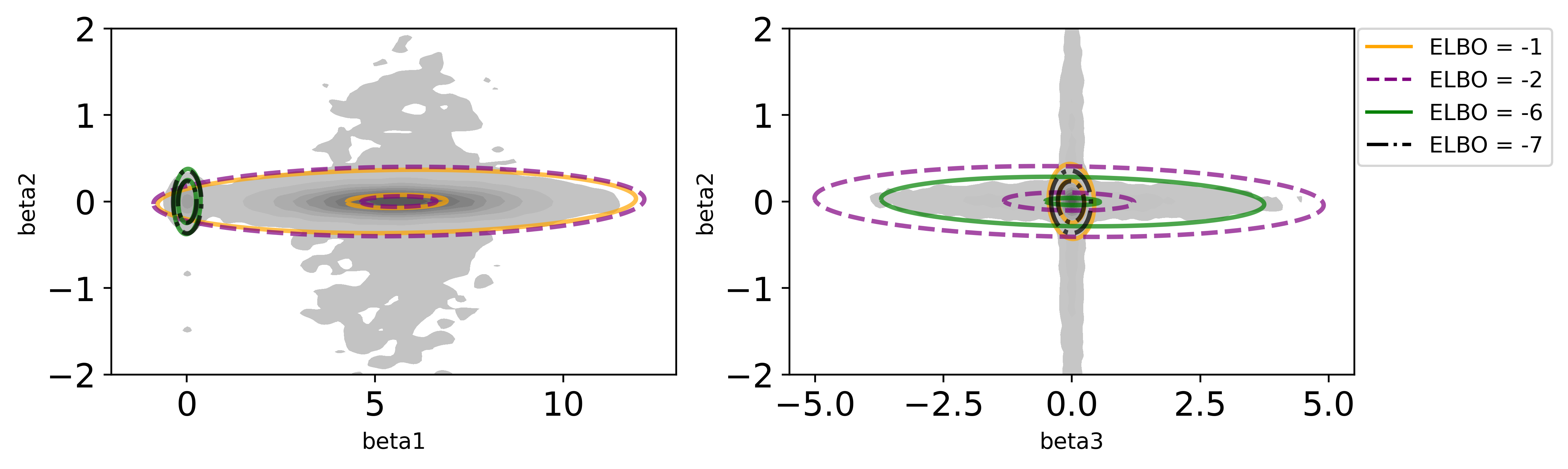
We use learning rates of γk=0.01\gamma_{k}=0.01 for the optimization of SMAP, t=0.01t=0.01 for backtracking line search, and set the smoothing constant αn=2\alpha_{n}=2. Both the initial value of SMAP optimization, MAP optimization and the mean initialization of SVI are randomly sampled from the prior distribution. In terms of L0L_{0}, we consider two different initialization schemes—the identity matrix and a random diagonal matrix—for both CSVI and SVI, where for the random L0L_{0}, log⁡[L0]i​i,i∈[d]\log\left[L_{0}\right]_{ii},i\in[d] is uniform in the range (log⁡0.1,log⁡100)(\log 0.1,\log 100). The learning rates for both VI algorithms are set to 0.0010.001. Fig. 9 shows the ELBOs of VI inference on the synthetic data over 100100 trials. Compared to SVI, CSVI reliably learns a better approximation to the posterior and rarely gets trapped at a local optimum. And CLA is much more robust to local minima compared to standard Laplace due to a good initialization. To visualize different Gaussian approximation, Fig. 10 shows contours of the optimal variational approximation (ELBO=−1\text{ELBO}=-1) and three local approximations corresponding to ELBO=−2,−6,−7\text{ELBO}=-2,-6,-7 respectively; it is clear that CSVI tends to find better local optima than SVI. Notice that in this example, the ELBO distribution of CLA is more consistent than CSVI’s. This is essentially due to the fact that CLA is a deterministic approximation methods—the Hessian of log posterior evaluated at the mean determines the fitted covariance, while CSVI is able to produce multiple covariance fit given the Gaussian mean.

For the real dataset experiment, we subsample the original dataset to N=30N=30 data points. We apply the SMAP optimization for 200,000200{,}000 iterations with the smoothing constant αn=0.03\alpha_{n}=0.03; and the learning rate for SMAP and VI algorithms are set as 0.0020.002 and 0.00020.0002 respectively. Other settings remain identical to the synthetic experiment. The results in Fig. 11 generally align with those from the previous synthetic experiment—CSVI and CLA outperform SVI and Laplace respetively with a more consistent and accurate Gaussian approximation. But an interesting observation is that CLA dominates all other methods and CSVI fails to learn those Gaussian disitrbuiton produced by CLA. It is mainly because that CLA fits into the dominating mode of posterior while CSVI prefers to fit a wider Gaussian distribution that covers the whole range of the posterior. A more detailed discussion, including several supporting visualizations is included in Section A.3.

Refer to caption
Figure 9: Sparse regression results on the synthetic dataset. The violin plots show the distribution of the ELBOs over 100100 trials.
Refer to caption
Figure 10: Visualization of different VI approximations to the posterior distribution on synthetic dataset (β1​v.s.​β2\beta_{1}\text{v.s.}\beta_{2}; β3​v.s.​β2\beta_{3}\text{v.s.}\beta_{2} ).The grey area depicts the posterior density and four Gaussian approximations displayed in contour plots corresponding to different ELBOs.
Refer to caption
Figure 11: Sparse regression results on the prostate cancer dataset. The violin plots show the distribution of the ELBOs over 100100 trials.

5.3 Bayesian Gaussian mixture model

Refer to caption
Figure 12: Synthetic dataset of GMM.
Refer to caption
(a) (a)
Refer to caption
(b) (b)
Figure 13: GMM results on the synthetic dataset Fig. 13(a) and real dataset Fig. 13(b). The violin plots show the distribution of the ELBOs over 100100 trials.

We finally compare the methods on a Bayesian Gaussian mixture model (GMM) applied to a synthetic dataset and the Shapley galaxy dataset 44 4 This dataset contains the measurements of the redshifts for 42154215 galaxies in the Shapley Concentration regions and was generously made available by Michael Drinkwater, University of Queensland, which can be downloaded from https://astrostatistics.psu.edu/datasets/Shapley_galaxy.html .. Similar to the previous experiments, we employ Adam for all optimization procedures involved in the inference and each experiment is repeated for 100100 trials. In the Bayesian Gaussian mixture model, we are given NN observations (xn)n=1N⊆ℝd(x_{n})^{N}_{n=1}\subseteq\mathbb{R}^{d}, each following a kk-component Gaussian mixture distribution:

xn|θ1:K,μ1:K,σ1:K,1:D\displaystyle x_{n}|\theta_{1:K},\mu_{1:K},\sigma_{1:K,1:D} ∼∑k=1Kθk​𝒩​(μk,diag⁡(σk​1,…,σk​D)).\displaystyle\sim\sum_{k=1}^{K}\theta_{k}\mathcal{N}\left(\mu_{k},\operatorname{diag}(\sigma_{k1},\dots,\sigma_{kD})\right). (61)

The goal is to infer the posterior distribution of all the latent parameters (θ1:k,μ1:k,σ1:K,1:D)(\theta_{1:k},\mu_{1:k},\sigma_{1:K,1:D}), on which we place a Dirichlet prior on the mixture proportions, a Gaussian prior on the Gaussian means, and a lognormal prior on the standard deviations, i.e.,

(θ1,…,θK)\displaystyle(\theta_{1},\dots,\theta_{K}) ∼𝖣𝗂𝗋⁡(α0)\displaystyle\sim{\sf{Dir}}(\alpha_{0}) (62)
μk\displaystyle\mu_{k} ∼𝒩(0,I),k=1,2,…,K\displaystyle\sim\mathcal{N}(0,I),\quad k=1,2,\dots,K (63)
σk​d\displaystyle\sigma_{kd} ∼𝖫𝗈𝗀𝖭𝗈𝗋𝗆𝖺𝗅⁡(0,1),\displaystyle\sim{\sf{LogNormal}}(0,1), (64)
k=1,2,…,K,d=1,2,…​D.\displaystyle\qquad k=1,2,\dots,K,d=1,2,\dots D. (65)

One may notice that the support of θk\theta_{k} and σk​d\sigma_{kd} is constrained; the present work is limited to posterior distributions with full support. Therefore, we first apply transformations such that the transformed random variables have unconstrained support Kucukelbir et al. 2017. The details of the transformation can be found in Section A.4.1.

For the synthetic dataset, we generate N=400N=400 data points equally from 44 isotropic bivariate Gaussian distributions with equal covariance 0.62​I0.6^{2}I. The mean of those Gaussian distributions are generated randomly within [−10,10]2[-10,10]^{2}. Fig. 12 displays the synthetic data points, where samples from the four Gaussian distributions are distinguished by different colors. We fit this dataset with K=3K=3 and set α0=1\alpha_{0}=1—we pick a misspecified setting to make the posterior distribution have multiple meaningful modes and hence create local optima for GVB inference. During inference, we use samples from the prior distribution as the initial value for SMAP, Laplace and the mean for SVI. The smoothing constant for smoothed MAP estimator is set to 11. For the initialization of covariance matrix, we set L0=IL_{0}=I for CSVI and use two different settings for SVI; we consider both the identity matrix and random diagonal matrix, of which the log diagonal indices are uniformly sampled in the range (log⁡0.1,log⁡100)(\log 0.1,\log 100). We use a learning rate γk=0.1\gamma_{k}=0.1 for SMAP and γk=0.01\gamma_{k}=0.01 for both VI algorithms. The initial step size tt for the line search of Laplace is set to 11. The experimental results are illustrated in Fig. 13(a), from which we notice that CSVI and CLA are able to consistently find the global optimum in almost every trial while both SVI and Laplace tends to converge to some local optima. A similar phenomenon is also observed in the real data experiment (Fig. 13(b)), suggesting that CSVI is more reliable. But in this case, though CLA is noticabily better than the standard Laplace approxiamtion, it is outperformed by all variational inference methods. This reveals the limitation of Laplace approximation—it is a local approximation method which totally depends on the curvature of log posterior function; while variational inference is based on reducing KL divergence to the target, which is a gloabl metric. The details of the real data experiment are deferred to Section A.4.2.

6 Conclusion

This work provides an extensive theoretical analysis of the computational aspects of Laplace approximation and Guassian variational inference, and uses the theory to design a general procedure that addresses the nonconvexity of the problem in an asymptotic regime. We show that under mild conditions, the MAP estimation problem and Gaussian variational optimization are locally asymptotically convex. Based on this fact, we developed consistent stochastic variational inference (CSVI), a scheme that asymptotically solves Gaussian variational inference; and consistent Laplace approximation, a variant of Laplace approximation that address the intractability of finding MAP value. Both CSVI and CLA solves a smoothed MAP problem to initialize the Gaussian mean within the locally convex area, and then CSVI further runs a scaled projected stochastic gradient descent to create iterates that converge to the optimum. The asymptotic consistency of CSVI is mathematically justified, and experimental results demonstrate the advantages over traditional SVI.

There are many avenues of further exploration for the present work. For example, we limit consideration to the case of Gaussian variational families due to their popularity; but aside from the mathematical details, nothing about the overall strategy necessarily relied on this choice. It would be worth examining other popular variational families, such as mean-field exponential families (Xing et al. 2002).

Furthermore, the current work is limited to posterior distributions with full support on ℝd\mathbb{R}^{d}—otherwise, the KL divergence variational objective is degenerate. It would be of interest to study whether variational inference using a Gaussian variational family truncated to the support of the posterior possesses the same beneficial asymptotic properties and asymptotically consistent optimization algorithm as developed in the present work.

Another interesting potential line of future work is to investigate other probability measure divergences as variational objectives. For example, the chi-square divergence (Liese and Vajda 1987; Csiszár 1967, p. 51), Rényi α\alpha-divergence (Van Erven and Harremos 2014), Stein discrepancy (Stein 1972), and more (Gibbs and Su 2002) have all been used as variational objectives. Along a similar vein, we studied the convergence properties of only a relatively simple stochastic gradient descent algorithm; other base algorithms with better convergence properties exist (Kingma and Ba 2015; Duchi et al. 2011; Nesterov 1983), and it may be fruitful to see if they have similar asymptotic consistency properties.

A final future direction is to investigate the asymptotic behaviour of variational inference with respect to other measures of optimization tractability. In particular, (local) pseudoconvexity (Crouzeix and Ferland 1982), quasiconvexity (Arrow and Enthoven 1961), and invexity (Ben-Israel and Mond 1986; Craven and Glover 1985) are all weaker than (local) convexity, but provide similar guarantees for stochastic optimization. These may be necessary to consider when examining other divergences as variational objectives.

Acknowledgements.
The authors gratefully acknowledge the support of an Natural Sciences and Engineering Research Council of Canada (NSERC) Discovery Grant and Discovery Launch Supplement, and UBC four year doctoral fellowship.

References

  • Addis et al. (2005) Addis B, Locatelli M, Schoen F (2005) Local optima smoothing for global optimization. Optimization Methods and Software 20(4-5):417–437
  • Alquier and Ridgway (2020) Alquier P, Ridgway J (2020) Concentration of tempered posteriors and of their variational approximations. The Annals of Statistics 48(3):1475–1497
  • Armijo (1966) Armijo L (1966) Minimization of functions having Lipschitz continuous first partial derivatives. Pacific Journal of mathematics 16(1):1–3
  • Arrow and Enthoven (1961) Arrow K, Enthoven A (1961) Quasi-concave programming. Econometrica: Journal of the Econometric Society pp 779–800
  • Balakrishnan et al. (2017) Balakrishnan S, Wainwright M, Yu B (2017) Statistical guarantees for the EM algorithm: From population to sample-based analysis. The Annals of Statistics 45(1):77–120
  • Barber et al. (2016) Barber RF, Drton M, Tan KM (2016) Laplace approximation in high-dimensional Bayesian regression. In: Statistical Analysis for High-Dimensional Data, Springer, pp 15–36
  • Bassett and Deride (2019) Bassett R, Deride J (2019) Maximum a posteriori estimators as a limit of Bayes estimators. Mathematical Programming 174(1-2):129–144
  • Bauschke and Combettes (2011) Bauschke H, Combettes P (2011) Convex Analysis and Monotone Operator Theory in Hilbert Spaces. Springer
  • Ben-Israel and Mond (1986) Ben-Israel A, Mond B (1986) What is invexity? The ANZIAM Journal 28(1):1–9
  • Bertsekas and Tsitsiklis (2000) Bertsekas D, Tsitsiklis J (2000) Gradient convergence in gradient methods with errors. SIAM Journal on Optimization 10(3):627–642
  • Bishop and Nasrabadi (2006) Bishop C, Nasrabadi N (2006) Pattern Recognition and Machine Learning. Springer
  • Blei et al. (2017) Blei D, Kucukelbir A, McAuliffe J (2017) Variational inference: A review for statisticians. Journal of the American Statistical Association 112(518):859–877
  • Bottou (2004) Bottou L (2004) Stochastic Learning. In: Bousquet O, von Luxburg U, Rätsch G (eds) Advanced Lectures on Machine Learning: ML Summer Schools 2003, Springer Berlin Heidelberg, pp 146–168
  • Boucheron et al. (2013) Boucheron S, Lugosi G, Massart P (2013) Concentration Inequalities: A Nonasymptotic Theory of Independence. Oxford university press
  • Boyd and Vandenberghe (2004) Boyd S, Vandenberghe L (2004) Convex Optimization. Cambridge University Press
  • Bubeck (2015) Bubeck S (2015) Convex Optimization: Algorithms and Complexity. Now Publishers Inc
  • Campbell and Li (2019) Campbell T, Li X (2019) Universal boosting variational inference. In: Advances in Neural Information Processing Systems
  • Craven and Glover (1985) Craven B, Glover B (1985) Invex functions and duality. Journal of the Australian Mathematical Society 39(1):1–20
  • Crouzeix and Ferland (1982) Crouzeix JP, Ferland J (1982) Criteria for quasi-convexity and pseudo-convexity: relationships and comparisons. Mathematical Programming 23(1):193–205
  • Csiszár (1967) Csiszár I (1967) Information-type measures of difference of probability distributions and indirect observation. Studia Scientiarum Mathematicarum Hungarica 2:229–318
  • Duchi et al. (2011) Duchi J, Hazan E, Singer Y (2011) Adaptive subgradient methods for online learning and stochastic optimization. Journal of Machine Learning Research 12(7):2121–2159
  • Folland (1999) Folland G (1999) Real Analysis: Modern Techniques and their Applications. John Wiley & Sons
  • Forsyth and Ponce (2002) Forsyth D, Ponce J (2002) Computer Vision: a Modern Approach. Prentice Hall Professional Technical Reference
  • Gelfand and Smith (1990) Gelfand A, Smith A (1990) Sampling-based approaches to calculating marginal densities. Journal of the American Statistical Association 85(410):398–409
  • George and McCulloch (1993) George E, McCulloch R (1993) Variable selection via Gibbs sampling. Journal of the American Statistical Association 88(423):881–889
  • Ghosal et al. (2000) Ghosal S, Ghosh J, van der Vaart A (2000) Convergence rates of posterior distributions. The Annals of Statistics 28(2):500–531
  • Gibbs and Su (2002) Gibbs A, Su FE (2002) On choosing and bounding probability metrics. International Statistical Review 70(3):419–435
  • Grendár and Judge (2009) Grendár M, Judge G (2009) Asymptotic equivalence of empirical likelihood and Bayesian MAP. The Annals of Statistics pp 2445–2457
  • Guo et al. (2016) Guo F, Wang X, Fan K, Broderick T, Dunson D (2016) Boosting variational inference. In: Advances in Neural Information Processing Systems
  • Haddad and Akansu (1991) Haddad R, Akansu A (1991) A class of fast Gaussian binomial filters for speech and image processing. IEEE Transactions on Signal Processing 39(3):723–727
  • Hall et al. (2011) Hall P, Pham T, Wand M, Wang SS (2011) Asymptotic normality and valid inference for gaussian variational approximation. The Annals of Statistics 39(5):2502–2532
  • Han and Yang (2019) Han W, Yang Y (2019) Statistical inference in mean-field variational Bayes. arXiv: 1911.01525
  • Hastings (1970) Hastings W (1970) Monte Carlo sampling methods using Markov chains and their applications. Biometrika 57(1):97–109
  • Hoffman et al. (2013) Hoffman M, Blei D, Wang C, Paisley J (2013) Stochastic variational inference. The Journal of Machine Learning Research 14(1):1303–1347
  • Huggins et al. (2020) Huggins J, Kasprzak M, Campbell T, Broderick T (2020) Validated variational inference via practical posterior error bounds. In: International Conference on Artificial Intelligence and Statistics
  • Ionides (2008) Ionides E (2008) Truncated importance sampling. Journal of Computational and Graphical Statistics 17(2):295–311
  • Jaiswal et al. (2019) Jaiswal P, Rao V, Honnappa H (2019) Asymptotic consistency of α−\alpha-Rényi-approximate posteriors. arXiv: 1902.01902
  • Jennrich (1969) Jennrich R (1969) Asymptotic properties of non-linear least squares estimators. The Annals of Mathematical Statistics 40(2):633–643
  • Jordan et al. (1998) Jordan M, Ghahramani Z, Jaakkola T, Saul L (1998) An introduction to variational methods for graphical models. In: Learning in Graphical Models, Springer, pp 105–161
  • Kass (1990) Kass R (1990) The validity of posterior expansions based on Laplace’s method. Bayesian and likelihood methods in statistics and econometrics pp 473–487
  • Kingma and Ba (2015) Kingma D, Ba J (2015) Adam: A method for stochastic optimization. In: International Conference on Learning Representations
  • Kingma and Welling (2014) Kingma D, Welling M (2014) Auto-encoding variational Bayes. In: International Conference on Learning Representations
  • Kleijn (2004) Kleijn B (2004) Bayesian asymptotics under misspecification. PhD thesis, Vrije Universiteit Amsterdam
  • Kleijn and van der Vaart (2012) Kleijn B, van der Vaart A (2012) The Bernstein-von-Mises theorem under misspecification. Electronic Journal of Statistics 6:354–381
  • Kontorovich (2014) Kontorovich A (2014) Concentration in unbounded metric spaces and algorithmic stability. In: International Conference on Machine Learning
  • Kucukelbir et al. (2017) Kucukelbir A, Tran D, Ranganath R, Gelman A, Blei D (2017) Automatic differentiation variational inference. The Journal of Machine Learning Research 18(1):430–474
  • LeCam (1960) LeCam L (1960) Locally Asymptotically Normal Families of Distributions. Berkeley: University of California Press
  • Liese and Vajda (1987) Liese F, Vajda I (1987) Convex Statistical Distances. Teubner
  • Lindeberg (1990) Lindeberg T (1990) Scale-space for discrete signals. IEEE Transactions on Pattern Analysis and Machine Intelligence 12(3):234–254
  • Locatello et al. (2018) Locatello F, Dresdner G, Khanna R, Valera I, Rätsch G (2018) Boosting black box variational inference. In: Advances in Neural Information Processing Systems
  • Meyn and Tweedie (2012) Meyn S, Tweedie R (2012) Markov Chains and Stochastic Stability. Springer Science & Business Media
  • Miller et al. (2017) Miller A, Foti N, Adams R (2017) Variational boosting: Iteratively refining posterior approximations. In: International Conference on Machine Learning
  • Miller (2021) Miller J (2021) Asymptotic normality, concentration, and coverage of generalized posteriors. Journal of Machine Learning Research 22(168):1–53
  • Mobahi (2013) Mobahi H (2013) Optimization by Gaussian smoothing with application to geometric alignment. PhD thesis, University of Illinois at Urbana-Champaign
  • Murphy (2012) Murphy K (2012) Machine Learning: A Probabilistic Perspective. MIT Press
  • Nesterov (1983) Nesterov Y (1983) A method of solving a convex programming problem with convergence rate O⁡(k2){O}(k^{2}). In: Doklady Akademii Nauk
  • Nixon and Aguado (2012) Nixon M, Aguado A (2012) Feature Extraction and Image Processing for Computer Vision. Academic Press
  • Pinheiro and Bates (1996) Pinheiro J, Bates D (1996) Unconstrained parametrizations for variance-covariance matrices. Statistics and Computing 6:289–296
  • Qiao and Minematsu (2010) Qiao Y, Minematsu N (2010) A study on invariance of ff-divergence and its application to speech recognition. IEEE Transactions on Signal Processing 58(7):3884–3890
  • Rakhlin et al. (2012) Rakhlin A, Shamir O, Sridharan K (2012) Making gradient descent optimal for strongly convex stochastic optimization. In: International Coference on International Conference on Machine Learning
  • Ranganath (2014) Ranganath R (2014) Black box variational inference. In: Advances in Neural Information Processing Systems
  • Robbins and Monro (1951) Robbins H, Monro S (1951) A stochastic approximation method. The Annals of Mathematical Statistics pp 400–407
  • Robert and Casella (2013) Robert C, Casella G (2013) Monte Carlo Statistical Methods. Springer Science & Business Media
  • Roberts and Rosenthal (2004) Roberts G, Rosenthal J (2004) General state space Markov chains and MCMC algorithms. Probability surveys 1:20–71
  • Ryu and Boyd (2016) Ryu E, Boyd S (2016) Primer on monotone operator methods. Applied and Computational Mathematics 15(1):3–43
  • Schatzman (2002) Schatzman M (2002) Numerical Analysis: a Mathematical Introduction. Clarendon Press, translation: John Taylor
  • Schillings et al. (2020) Schillings C, Sprungk B, Wacker P (2020) On the convergence of the Laplace approximation and noise-level-robustness of Laplace-based Monte Carlo methods for Bayesian inverse problems. Numerische Mathematik 145(4):915–971
  • Shen and Wasserman (2001) Shen X, Wasserman L (2001) Rates of convergence of posterior distributions. The Annals of Statistics 29(3):687–714
  • Shun and McCullagh (1995) Shun Z, McCullagh P (1995) Laplace approximation of high dimensional integrals. Journal of the Royal Statistical Society: Series B (Methodological) 57(4):749–760
  • Stein (1972) Stein C (1972) A bound for the error in the normal approximation to the distribution of a sum of dependent random variables. In: Proceedings of the Sixth Berkeley Symposium on Mathematical Statistics and Probability
  • van der Vaart (2000) van der Vaart A (2000) Asymptotic Statistics. Cambridge University Press
  • van der Vaart and Wellner (2013) van der Vaart A, Wellner J (2013) Weak Convergence and Empirical Processes: with Applications to Statistics. Springer Science & Business Media
  • Van Erven and Harremos (2014) Van Erven T, Harremos P (2014) Rényi divergence and Kullback-Leibler divergence. IEEE Transactions on Information Theory 60(7):3797–3820
  • Vehtari et al. (2015) Vehtari A, Simpson D, Gelman A, Yao Y, Gabry J (2015) Pareto smoothed importance sampling. arXiv: 1507.02646
  • Wainwright and Jordan (2008) Wainwright M, Jordan M (2008) Graphical Models, Exponential Families, and Variational Inference. Now Publishers Inc
  • Wang and Blei (2019) Wang Y, Blei D (2019) Frequentist consistency of variational Bayes. Journal of the American Statistical Association 114(527):1147–1161
  • Xing et al. (2002) Xing E, Jordan M, Russell S (2002) A generalized mean field algorithm for variational inference in exponential families. In: Uncertainty in Artificial Intelligence
  • Yang et al. (2020) Yang Y, Pati D, Bhattacharya A (2020) α\alpha-variational inference with statistical guarantees. The Annals of Statistics 48(2):886–905
  • Zhang and Gao (2020) Zhang F, Gao C (2020) Convergence rates of variational posterior distributions. The Annals of Statistics 48(4):2180–2207

Appendix A Details of experiments

A.1 Details of the toy example for smoothed MAP

The underlying synthetic model for Fig. 1 is as follows,

θ∼15​𝒩​(0,0.152)+15​𝒩​(1,0.12)+15​𝒩​(−4,0.32)+15​𝒩​(4,0.32)\displaystyle\theta\sim\frac{1}{5}\mathcal{N}(0,0.15^{2})+\frac{1}{5}\mathcal{N}(1,0.1^{2})+\frac{1}{5}\mathcal{N}(-4,0.3^{2})+\frac{1}{5}\mathcal{N}(4,0.3^{2}) (66)
+15​𝒩​(−8,0.12)\displaystyle\quad+\frac{1}{5}\mathcal{N}(-8,0.1^{2}) (67)
Xi|θ​∼i.i.d. ​𝒩​(θ,5000),\displaystyle X_{i}\,|\,\theta\overset{\textrm{\tiny{i.i.d.}{} }}{\sim}\mathcal{N}(\theta,5000), (68)

where the data are truly generated from (Xi)i=1n​∼i.i.d. ​𝒩​(3,10)(X_{i})_{i=1}^{n}\overset{\textrm{\tiny{i.i.d.}{} }}{\sim}\mathcal{N}(3,10). For smoothed MAP optimization, we use a smoothing constant of αn=10​n−0.3\alpha_{n}=10n^{-0.3}, and set the initial value uniformly within the range (−50,50)(-50,50). The learning rate for the SGD is chosen as γk=15/(1+k0.9)\gamma_{k}=15/(1+k^{0.9}).

A.2 Algorithm: CSVI (Adam)

Algorithm 4 CSVI with adaptive moment estimation
procedure CSVI(fnf_{n}, gg, γ\gamma, KK)
  μ0←\mu_{0}\leftarrowSmoothedMAP (Algorithm 1), L0←IL_{0}\leftarrow I
  ϵ←10−8\epsilon\leftarrow 10^{-8}, β1←0.9\beta_{1}\leftarrow 0.9, β2←0.9999\beta_{2}\leftarrow 0.9999
  m0←0m_{0}\leftarrow 0, ν0←0\nu_{0}\leftarrow 0
  for k=0,1,…,K−1k=0,1,\dots,K-1 do ▶\blacktriangleright All operations on vector/matrix are elementwise
   Sample Zk∼𝒩⁡(0,I)Z_{k}\sim\mathcal{N}(0,I)
   gk←(∇^μ,n​(μk,Lk,Zk),∇~L,n​(μk,Lk,Zk))g_{k}\leftarrow\left(\hat{\nabla}_{\mu,n}(\mu_{k},L_{k},Z_{k}),\tilde{\nabla}_{L,n}(\mu_{k},L_{k},Z_{k})\right) ▶\blacktriangleright ∇^μ,n,∇~L,n\hat{\nabla}_{\mu,n},\tilde{\nabla}_{L,n} are same to Algorithm 3
   mk+1←β1​mk+(1−β1)​gkm_{k+1}\leftarrow\beta_{1}m_{k}+(1-\beta_{1})g_{k}
   vk+1←β2​vk+(1−β2)​gk2v_{k+1}\leftarrow\beta_{2}v_{k}+(1-\beta_{2})g_{k}^{2}
   m^k+1←mk/(1−β1k)\hat{m}_{k+1}\leftarrow m_{k}/(1-\beta_{1}^{k})
   v^k+1←vk/(1−β2k)\hat{v}_{k+1}\leftarrow v_{k}/(1-\beta_{2}^{k})
   (μk+1,Lk+1)←(μk,Lk)−γ​m^k/(v^k+ϵ)\left(\mu_{k+1},L_{k+1}\right)\leftarrow\left(\mu_{k},L_{k}\right)-\gamma\hat{m}_{k}/\left(\sqrt{\hat{v}_{k}}+\epsilon\right)
   for i=1,…,di=1,\dots,d do
     Lk+1,i​i←max⁡{0,Lk+1,i​i}L_{k+1,ii}\leftarrow\max\left\{0,L_{k+1,ii}\right\}
   end for
  end for
  return μK,LK\mu_{K},L_{K}
end procedure

A.3 Discussion of sparse regression experiment

In this section, we provide further discussion to the result presented in Fig. 11. Figs. 14 and 15 visualizes the Gaussian approximations produced by CLA and CSVI. Instead of fitting a single mode, CSVI covers the range of posterior and fit a Gaussian distribution with larger variance. Even though the performance of CSVI is consistent across runs, it does find the local optimum instead of the global solution. In this case, reverse KL—the objective function of Gaussian VI—can be limited. We compare the forward KL of these fitted Gaussians using 3200032000 posterior samples obatined from Stan, suggesting that CSVI find a solution that is better in forward KL.

Refer to caption
Figure 14: Visualization of different CLA approximations to the posterior distribution on real dataset.The grey area depicts the posterior density and four Gaussian approximations displayed in contour plots corresponding to different ELBOs.
Refer to caption
Figure 15: Visualization of different CSVI approximations to the posterior distribution on real dataset.The grey area depicts the posterior density and four Gaussian approximations displayed in contour plots corresponding to different ELBOs.
Refer to caption
Figure 16: Comparison of forward KL of sparse regression experiment

A.4 Details of the GMM experiment

A.4.1 Variable transformations of Bayesian Gaussian mixture model

To transform (θ1,…,θK)∈Δ⁡(K)(\theta_{1},\dots,\theta_{K})\in\Delta(K) and σk​d∈ℝ+\sigma_{kd}\in\mathbb{R}_{+} into unconstrained space, we consider the change of random variables as below:

  1. 1.

    For σk​d∼𝖫𝗈𝗀𝖭𝗈𝗋𝗆𝖺𝗅⁡(0,1)\sigma_{kd}\sim{\sf{LogNormal}}(0,1), we consider

    τk​d=log⁡(σk​d)∼𝒩⁡(0,1),\displaystyle\tau_{kd}=\log(\sigma_{kd})\sim\mathcal{N}(0,1), (69)

    which has a full support on ℝ\mathbb{R}.

  2. 2.

    For θ∼𝖣𝗂𝗋⁡(α0)\theta\sim{\sf{Dir}}(\alpha_{0}), we consider using marginalized LogGamma random variables. Notice the relationship of Gamma distribution and Dirichlet distirbution as follows,

    (λk)k=1K​∼i.i.d. ​𝖫𝗈𝗀𝖦𝖺𝗆𝗆𝖺​(α0,1)\displaystyle\left(\lambda_{k}\right)_{k=1}^{K}\overset{\textrm{\tiny{i.i.d.}{} }}{\sim}{\sf{LogGamma}}(\alpha_{0},1) (70)
    (exp⁡(λ1)∑kexp⁡(λk),…,exp⁡(λK)∑kexp⁡(λk))∼𝖣𝗂𝗋⁡(α0),\displaystyle\left(\frac{\exp(\lambda_{1})}{\sum_{k}\exp(\lambda_{k})},\dots,\frac{\exp(\lambda_{K})}{\sum_{k}\exp(\lambda_{k})}\right)\sim{\sf{Dir}}(\alpha_{0}), (71)

    then λk\lambda_{k} is supported on ℝ\mathbb{R}.

Therefore, instead of inferring the original parameters, we perform Gaussian variational inference on the posterior distribution of (λ1:k,μ1:k,τ11:k​d)(\lambda_{1:k},\mu_{1:k},\tau_{11:kd}).

A.4.2 Detailed settings for real data experiment

We subsample the Shapley galaxy dataset to N=500N=500 and the goal is to cluster the distribution of galaxies in the Shapley Concentration region. In our experiment, we fix the number of component K=3K=3 and set α0=1\alpha_{0}=1. During inference, we initialize the SMAP with random samples from the prior distribution, which are also used as the mean initialization for SVI. In SMAP, we perform the smoothed MAP estimation to a tempered posterior distribution πnκ\pi_{n}^{\kappa} with κ=1/2\kappa=1/2; and set the smoothing constant αn=3\alpha_{n}=3. The learning rate for SMAP and VI algorithms are chosen as 0.0050.005 and 0.0010.001 respectively. And similar to the synthetic experiment, CSVI and SVI_Ind use the identity matrix for L0L_{0} and SVI use random diagonal matrix for L0L_{0}, whose log diagonal indices are uniformly in the range (log⁡0.1,log⁡100)(\log 0.1,\log 100).

Appendix B Proofs

B.1 Proof of 6

Proof.

We consider the KL cost for the scaled and shifted posterior distribution. Let Π~n\tilde{\Pi}_{n} be the Bayesian posterior distribution of n​(θ−θ0)\sqrt{n}(\theta-\theta_{0}). The KL divergence measures the difference between the distributions of two random variables and is invariant when an invertible transformation is applied to both random variables (Qiao and Minematsu 2010, Theorem 1). Note that Π~n\tilde{\Pi}_{n} is shifted and scaled from Πn\Pi_{n}, and that this linear transformation is invertible, so

DKL(𝒩(μ,Σ)||Πn)=DKL(𝒩(n(μ−θ0),nΣ)||Π~n).\displaystyle\mathrm{D_{KL}}\left(\mathcal{N}(\mu,\Sigma)||\Pi_{n}\right)=\mathrm{D_{KL}}\left(\mathcal{N}\left(\sqrt{n}(\mu-\theta_{0}),n\Sigma\right)||\tilde{\Pi}_{n}\right). (72)

Let μ~n⋆,Σ~n⋆\tilde{\mu}_{n}^{\star},\tilde{\Sigma}_{n}^{\star} be the parameters of the optimal Gaussian variational approximation to Π~n\tilde{\Pi}_{n}, i.e.,

μ~n⋆,Σ~n⋆=arg​minμ∈ℝd,Σ∈ℝd×dDKL(𝒩(μ,Σ)||Π~n)s.t.Σ≻0,\displaystyle\tilde{\mu}_{n}^{\star},\tilde{\Sigma}_{n}^{\star}=\operatornamewithlimits{arg\,min}_{\mu\in\mathbb{R}^{d},\Sigma\in\mathbb{R}^{d\times d}}\mathrm{D_{KL}}\left(\mathcal{N}(\mu,\Sigma)||\tilde{\Pi}_{n}\right)\quad\text{s.t.}\quad\Sigma\succ 0, (73)

and let

𝒩n~⋆:=𝒩⁡(μ~n⋆,Σ~n⋆)=𝒩⁡(n​(μn⋆−θ0),Ln⋆​Ln⋆T).\displaystyle\tilde{\mathcal{N}_{n}}^{\star}:=\mathcal{N}\left(\tilde{\mu}_{n}^{\star},\tilde{\Sigma}_{n}^{\star}\right)=\mathcal{N}\left(\sqrt{n}(\mu_{n}^{\star}-\theta_{0}),L_{n}^{\star}L_{n}^{\star T}\right). (74)

Wang and Blei 2019 shows that under 1,

DTV​(𝒩n~⋆,𝒩⁡(Δn,θ0,Hθ0−1))→Pθ00.\displaystyle\mathrm{D_{TV}}\left(\tilde{\mathcal{N}_{n}}^{\star},\mathcal{N}\left(\Delta_{n,\theta_{0}},H_{\theta_{0}}^{-1}\right)\right)\stackrel{{\scriptstyle P_{\theta_{0}}}}{{\to}}0. (75)

Convergence in total variation implies weak convergence, which then implies pointwise convergence of the characteristic function. Denote ϕ~n⋆​(t)\tilde{\phi}^{\star}_{n}(t) and ϕn​(t)\phi_{n}(t) to be the characteristic functions of 𝒩n⋆~\tilde{\mathcal{N}_{n}^{\star}} and 𝒩⁡(Δn,θ0,Hθ0−1)\mathcal{N}\left(\Delta_{n,\theta_{0}},H_{\theta_{0}}^{-1}\right). Therefore

∀t∈ℝd,ϕn⋆​(t)ϕn​(t)\displaystyle\forall t\in\mathbb{R}^{d},\;\frac{\phi^{\star}_{n}(t)}{\phi_{n}(t)} =exp⁡(i​(n​(μn⋆−θ0)−Δn,θ0)T​t−12​tT​(Ln⋆​Ln⋆T−Hθ0−1)​t)\displaystyle=\exp\!\left(i(\sqrt{n}(\mu^{\star}_{n}-\theta_{0})-\Delta_{n,\theta_{0}})^{T}t-\frac{1}{2}t^{T}\left(L_{n}^{\star}L_{n}^{\star T}-H_{\theta_{0}}^{-1}\right)t\right) (76)
⟶Pθ01,\displaystyle\stackrel{{\scriptstyle P_{\theta_{0}}}}{{\longrightarrow}}1, (77)

which implies

μn⋆→Pθ01n​Δn,θ0+θ0,andLn⋆​Ln⋆T→Pθ0H0−1=L0​L0T.\displaystyle\mu_{n}^{\star}\stackrel{{\scriptstyle P_{\theta_{0}}}}{{\rightarrow}}\frac{1}{\sqrt{n}}\Delta_{n,\theta_{0}}+\theta_{0},\quad\text{and}\quad L_{n}^{\star}L_{n}^{\star T}\stackrel{{\scriptstyle P_{\theta_{0}}}}{{\rightarrow}}H^{-1}_{0}=L_{0}L_{0}^{T}. (78)

Under 1, van der Vaart 2000 states that

‖Δn,θ0−n​(θMLE,n−θ0)‖→Pθ00,\displaystyle\|\Delta_{n,\theta_{0}}-\sqrt{n}(\theta_{\text{MLE},n}-\theta_{0})\|\stackrel{{\scriptstyle P_{\theta_{0}}}}{{\to}}0, (79)

and θMLE,n​→Pθ0​θ0\theta_{\text{MLE},n}\overset{P_{\theta_{0}}}{\to}\theta_{0} according to Eq. 33, yielding μn⋆→Pθ0θ0\mu_{n}^{\star}\stackrel{{\scriptstyle P_{\theta_{0}}}}{{\to}}\theta_{0}.

Finally since the Cholesky decomposition defines a continuous mapping from the set of positive definite Hermitian matrices to the set of lower triangular matrices with positive diagonals (both sets are equipped with the spectral norm) (Schatzman 2002, p. 295), we have

Ln⋆→Pθ0L0.\displaystyle L_{n}^{\star}\stackrel{{\scriptstyle P_{\theta_{0}}}}{{\to}}L_{0}. (80)

∎

B.2 Proof of 11

Proof.

We provide a proof of the result for strong convexity; the result for Lipschitz smoothness follows the exact same proof technique. Note that if D′D^{\prime} does not depend on xx, Fn​(x)F_{n}(x) is D′D^{\prime}-strongly convex if and only if Fn​(x)−12​xT​D′​xF_{n}(x)-\frac{1}{2}x^{T}D^{\prime}x is convex. We use this equivalent characterization of strong convexity in this proof.

Note that for Z∼𝒩⁡(0,I)Z\sim\mathcal{N}(0,I),

𝔼[12(μ+n−1/2LZ)TD(μ+n−1/2LZ)]=12μTDμ+12trLT(n−1D)L.\displaystyle\mathbb{E}\left[\frac{1}{2}(\mu+n^{-1/2}LZ)^{T}D(\mu+n^{-1/2}LZ)\right]=\frac{1}{2}\mu^{T}D\mu+\frac{1}{2}\operatorname{tr}L^{T}(n^{-1}D)L. (81)

Define λ∈[0,1]\lambda\in[0,1], vectors μ,μ′∈ℝd\mu,\mu^{\prime}\in\mathbb{R}^{d}, positive-diagonal lower triangular matrices L,L′∈ℝd×dL,L^{\prime}\in\mathbb{R}^{d\times d}, and vectors x,x′∈ℝ(d+1)​dx,x^{\prime}\in\mathbb{R}^{(d+1)d} by stacking μ\mu and the columns of LL and likewise μ′\mu^{\prime} and the columns of L′L^{\prime}. Define x⁡(λ)=λ​x+(1−λ)​x′x(\lambda)=\lambda x+(1-\lambda)x^{\prime}, μ⁡(λ)=λ​μ+(1−λ)​μ′\mu(\lambda)=\lambda\mu+(1-\lambda)\mu^{\prime}, and L⁡(λ)=λ​L+(1−λ)​L′L(\lambda)=\lambda L+(1-\lambda)L^{\prime}. Then

Fn​(x⁡(λ))−12​x​(λ)T​diag⁡(D,n−1​D,…,n−1​D)​x​(λ)\displaystyle F_{n}(x(\lambda))-\frac{1}{2}x(\lambda)^{T}\operatorname{diag}(D,n^{-1}D,\dots,n^{-1}D)x(\lambda) (82)
=\displaystyle= Fn​(μ⁡(λ),L⁡(λ))−(12​μ​(λ)T​D​μ​(λ)+12​tr⁡L​(λ)T​(n−1​D)​L​(λ))\displaystyle F_{n}(\mu(\lambda),L(\lambda))-\left(\frac{1}{2}\mu(\lambda)^{T}D\mu(\lambda)+\frac{1}{2}\operatorname{tr}L(\lambda)^{T}(n^{-1}D)L(\lambda)\right) (83)
=\displaystyle= 𝔼[n−1logπn(μ(λ)+n−1/2L(λ)Z)−12(μ(λ)+n−1/2L(λ)Z)TD(μ(λ)\displaystyle\mathbb{E}\left[n^{-1}\log\pi_{n}(\mu(\lambda)+n^{-1/2}L(\lambda)Z)-\frac{1}{2}(\mu(\lambda)+n^{-1/2}L(\lambda)Z)^{T}D(\mu(\lambda)\right. (84)
+n−1/2L(λ)Z)].\displaystyle\left.+n^{-1/2}L(\lambda)Z)\right]. (85)

By the DD-strong convexity of n−1​log⁡πnn^{-1}\log\pi_{n},

≤\displaystyle\leq λ⁡(Fn​(μ,L)−12​μT​D​μ−12​tr⁡LT​(n−1​D)​L)\displaystyle\lambda\left(F_{n}(\mu,L)-\frac{1}{2}\mu^{T}D\mu-\frac{1}{2}\operatorname{tr}L^{T}(n^{-1}D)L\right) (86)
+(1−λ)​(Fn​(μ′,L′)−12​μ′T​D​μ′−12​tr⁡L′T​(n−1​D)​L′)\displaystyle+(1-\lambda)\left(F_{n}(\mu^{\prime},L^{\prime})-\frac{1}{2}\mu^{\prime T}D\mu^{\prime}-\frac{1}{2}\operatorname{tr}L^{\prime T}(n^{-1}D)L^{\prime}\right) (87)
=\displaystyle= λ⁡(Fn​(x)−12​xT​diag⁡(D,n−1​D,…,n−1​D)​x)\displaystyle\lambda\left(F_{n}(x)-\frac{1}{2}x^{T}\operatorname{diag}(D,n^{-1}D,\dots,n^{-1}D)x\right) (88)
+(1−λ)​(Fn​(x′)−12​x′T​diag⁡(D,n−1​D,…,n−1​D)​x′).\displaystyle+(1-\lambda)\left(F_{n}(x^{\prime})-\frac{1}{2}x^{\prime T}\operatorname{diag}(D,n^{-1}D,\dots,n^{-1}D)x^{\prime}\right). (89)

∎

B.3 Proof of 12

Proof.

Note that by reparameterization,

arg​minμDKL(𝒩(μ,σ2)||Πn)=arg​minμ𝔼[−n−1logπn(μ+σZ)],\displaystyle\operatornamewithlimits{arg\,min}_{\mu}\mathrm{D_{KL}}\left(\mathcal{N}(\mu,\sigma^{2})||\Pi_{n}\right)=\operatornamewithlimits{arg\,min}_{\mu}\mathbb{E}\left[-n^{-1}\log\pi_{n}(\mu+\sigma Z)\right], (90)

where Z∼𝒩⁡(0,1)Z\sim\mathcal{N}(0,1). Using a Taylor expansion,

−𝔼⁡[d2d​μ2​(−n−1​log⁡πn​(μ+σ​Z))]\displaystyle-\mathbb{E}\left[\frac{d^{2}}{d\mu^{2}}\left(-n^{-1}\log\pi_{n}(\mu+\sigma Z)\right)\right] (91)
=𝔼⁡[−n−1​log⁡πn(2)​(μ)−n−1​log⁡πn(3)​(μ′)⋅σ​Z],\displaystyle=\mathbb{E}\left[-n^{-1}\log\pi_{n}^{(2)}(\mu)-n^{-1}\log\pi_{n}^{(3)}(\mu^{\prime})\cdot\sigma Z\right], (92)

for some μ′\mu^{\prime} between μ\mu and μ+σ​Z\mu+\sigma Z. By the uniform bound on the third derivative and local bound on the second derivative, for any μ∈U\mu\in U,

𝔼⁡[−n−1​log⁡πn(2)​(μ)−n−1​log⁡πn(3)​(μ′)⋅σ​Z]\displaystyle\mathbb{E}\left[-n^{-1}\log\pi_{n}^{(2)}(\mu)-n^{-1}\log\pi_{n}^{(3)}(\mu^{\prime})\cdot\sigma Z\right] ≤−ϵ+η​σ​𝔼​|Z|\displaystyle\leq-\epsilon+\eta\sigma\mathbb{E}\left|Z\right| (93)
≤−ϵ+η​σ.\displaystyle\leq-\epsilon+\eta\sigma. (94)

The result follows for any 0<ϵ<ϵ/η0<\epsilon<\epsilon/\eta. ∎

B.4 Proof of 13

Proof.

Note that we can split LL into columns and express L​ZLZ as

L​Z=∑i=1dLi​Zi,\displaystyle LZ=\sum_{i=1}^{d}L_{i}Z_{i}, (95)

where Li∈ℝpL_{i}\in\mathbb{R}^{p} is the ithi^{\text{th}} column of LL, and (Zi)i=1d​∼i.i.d. ​𝒩​(0,1)(Z_{i})_{i=1}^{d}\overset{\textrm{\tiny{i.i.d.}{} }}{\sim}\mathcal{N}(0,1). Denoting ∇2fn:=∇2fn​(μ+L​Z)\nabla^{2}f_{n}:=\nabla^{2}f_{n}(\mu+LZ) for brevity, the 2nd2^{\text{nd}} derivatives in both μ\mu and LL are

∇μ​μ2Fn\displaystyle\nabla^{2}_{\mu\mu}F_{n} =𝔼⁡[∇2fn]\displaystyle=\mathbb{E}\left[\nabla^{2}f_{n}\right] (96)
∇Li​Lj2Fn\displaystyle\nabla^{2}_{L_{i}L_{j}}F_{n} =n−1​𝔼​[Zi​Zj​∇2fn]\displaystyle=n^{-1}\mathbb{E}\left[Z_{i}Z_{j}\nabla^{2}f_{n}\right] (97)
∇μ​Li2Fn\displaystyle\nabla^{2}_{\mu L_{i}}F_{n} =n−1/2𝔼[Zi∇2fn]\displaystyle=n^{-1/2}\mathbb{E}\left[Z_{i}\nabla^{2}f_{n}\right] (98)

where we can pass the gradient and Hessian through the expectation by dominated convergence because ZZ has a normal distribution and fnf_{n} has ℓ\ell-Lipschitz gradients. Stacking these together in block matrices yields the overall Hessian,

A\displaystyle A =[In−1/2Z1I…n−1/2ZdI]∈ℝd×d⁡(d+1)\displaystyle=\left[\begin{array}[]{cccc}I&n^{-1/2}Z_{1}I&\dots&n^{-1/2}Z_{d}I\end{array}\right]\in\mathbb{R}^{d\times d(d+1)}
∇2Fn\displaystyle\nabla^{2}F_{n} =𝔼⁡[AT​∇2fn​A]∈ℝd⁡(d+1)×d⁡(d+1).\displaystyle=\mathbb{E}\left[A^{T}\nabla^{2}f_{n}A\right]\in\mathbb{R}^{d(d+1)\times d(d+1)}. (100)

Since fnf_{n} has ℓ\ell-Lipschitz gradients, for all x∈ℝdx\in\mathbb{R}^{d}, −ℓ​I⪯∇2fn​(x)⪯ℓ​I-\ell I\preceq\nabla^{2}f_{n}(x)\preceq\ell I. Applying the upper bound and evaluating the expectation yields the Hessian upper bound (and the same technique yields the corresponding lower bound):

∇2Fn\displaystyle\nabla^{2}F_{n} =𝔼⁡[AT​∇2fn​A]\displaystyle=\mathbb{E}\left[A^{T}\nabla^{2}f_{n}A\right] (101)
⪯ℓ​𝔼​[AT​A]\displaystyle\preceq\ell\mathbb{E}\left[A^{T}A\right] (102)
=ℓ⁡[I0000n−1​I0000⋱0000n−1​I]=ℓ​Dn.\displaystyle=\ell\left[\begin{array}[]{cccc}I&0&0&0\\ 0&n^{-1}I&0&0\\ 0&0&\ddots&0\\ 0&0&0&n^{-1}I\end{array}\right]=\ell D_{n}.

To demonstrate local strong convexity, we split the expectation into two parts: one where n−1/2LZn^{-1/2}LZ is small enough to guarantee that ∥μ+n−1/2LZ−x∥2≤r2\|\mu+n^{-1/2}LZ-x\|^{2}\leq r^{2}, and the complement. Define

rn2​(μ,L):=n​(r2−2​‖μ−x‖22)2​‖L‖F2.\displaystyle r_{n}^{2}(\mu,L):=n\frac{(r^{2}-2\|\mu-x\|^{2}_{2})}{2\|L\|^{2}_{F}}. (107)

Note that when ‖Z‖2≤rn2​(μ,L)\|Z\|^{2}\leq r_{n}^{2}(\mu,L),

‖μ+1n​L​Z−x‖22\displaystyle\left\|\mu+\frac{1}{\sqrt{n}}LZ-x\right\|_{2}^{2} ≤2​‖μ−x‖2+2​n−1​‖L​Z‖2\displaystyle\leq 2\|\mu-x\|^{2}+2n^{-1}\|LZ\|^{2} (108)
≤2​‖μ−x‖2+2​n−1​‖L‖F2​‖Z‖2\displaystyle\leq 2\|\mu-x\|^{2}+2n^{-1}\|L\|_{F}^{2}\|Z\|^{2} (109)
≤r2.\displaystyle\leq r^{2}. (110)

Then we may write

∇2Fn\displaystyle\nabla^{2}F_{n} =𝔼[𝟙[∥Z∥2≤rn2(μ,L)]AT∇2fnA]\displaystyle=\mathbb{E}\left[\mathds{1}\left[\|Z\|^{2}\leq r_{n}^{2}(\mu,L)\right]A^{T}\nabla^{2}f_{n}A\right] (111)
+𝔼[𝟙[∥Z∥2>rn2(μ,L)]AT∇2fnA].\displaystyle\qquad+\mathbb{E}\left[\mathds{1}\left[\|Z\|^{2}>r_{n}^{2}(\mu,L)\right]A^{T}\nabla^{2}f_{n}A\right]. (112)

Since fnf_{n} has ℓ\ell-Lipschitz gradients and is locally ϵ\epsilon-strongly convex,

∇2Fn\displaystyle\nabla^{2}F_{n} ⪰ϵ⋅𝔼[𝟙[∥Z∥2≤rn2(μ,L)]ATA]−ℓ⋅𝔼[𝟙[∥Z∥2>rn2(μ,L)]ATA].\displaystyle\succeq\epsilon\cdot\mathbb{E}\left[\mathds{1}\left[\|Z\|^{2}\leq r_{n}^{2}(\mu,L)\right]A^{T}A\right]-\ell\cdot\mathbb{E}\left[\mathds{1}\left[\|Z\|^{2}>r_{n}^{2}(\mu,L)\right]A^{T}A\right]. (113)

Note that AT​AA^{T}A has entries 11 and n−1​Zi2n^{-1}Z_{i}^{2} along the diagonal, as well as n−1​Zi​Zjn^{-1}Z_{i}Z_{j}, i≠ji\neq j and n−1/2Zin^{-1/2}Z_{i} on the off-diagonals. By symmetry, since ZZ is an isotropic Gaussian, censoring by 𝟙[∥Z∥2≤…]\mathds{1}\left[\|Z\|^{2}\leq\dots\right] or 𝟙[∥Z∥2>…]\mathds{1}\left[\|Z\|^{2}>\dots\right] maintains that the off-diagonal expectations are 0. Therefore the quantity 𝔼[𝟙[∥Z∥2≤rn2(μ,L)]ATA]\mathbb{E}\left[\mathds{1}\left[\|Z\|^{2}\leq r_{n}^{2}(\mu,L)\right]A^{T}A\right] is diagonal with coefficients 1−αn​(μ,L)1-\alpha_{n}(\mu,L) and n−1​βn​(μ,L)n^{-1}\beta_{n}(\mu,L), and 𝔼[𝟙[∥Z∥2>rn2(μ,L)]ATA]\mathbb{E}\left[\mathds{1}\left[\|Z\|^{2}>r_{n}^{2}(\mu,L)\right]A^{T}A\right] is diagonal with coefficients αn​(μ,L)\alpha_{n}(\mu,L) and n−1​τn​(μ,L)n^{-1}\tau_{n}(\mu,L) where

αn​(μ,L)\displaystyle\alpha_{n}(\mu,L) =ℙ⁡(‖Z‖2>rn2​(μ,L))\displaystyle=\mathbb{P}\left(\|Z\|^{2}>r_{n}^{2}(\mu,L)\right) (114)
βn​(μ,L)\displaystyle\beta_{n}(\mu,L) =𝔼[Z12𝟙[∥Z∥2≤rn2(μ,L)]]=d−1𝔼[∥Z∥22𝟙[∥Z∥2≤rn2(μ,L)]]\displaystyle=\mathbb{E}\left[Z_{1}^{2}\mathds{1}\left[\|Z\|^{2}\leq r_{n}^{2}(\mu,L)\right]\right]=d^{-1}\mathbb{E}\left[\|Z\|_{2}^{2}\mathds{1}\left[\|Z\|^{2}\leq r_{n}^{2}(\mu,L)\right]\right] (115)
τn​(μ,L)\displaystyle\tau_{n}(\mu,L) =𝔼[Z12𝟙[∥Z∥2>rn2(μ,L)]]=d−1𝔼[∥Z∥22𝟙[∥Z∥2>rn2(μ,L)]].\displaystyle=\mathbb{E}\left[Z_{1}^{2}\mathds{1}\left[\|Z\|^{2}>r_{n}^{2}(\mu,L)\right]\right]=d^{-1}\mathbb{E}\left[\|Z\|_{2}^{2}\mathds{1}\left[\|Z\|^{2}>r_{n}^{2}(\mu,L)\right]\right]. (116)

Note that ‖Z‖2∼χd2\|Z\|^{2}\sim\chi^{2}_{d}; so αn​(μ,L)=1−χd2​(rn2​(μ,L))\alpha_{n}(\mu,L)=1-\chi^{2}_{d}(r_{n}^{2}(\mu,L)) and

τn​(μ,L)\displaystyle\tau_{n}(\mu,L) =∫rn2​(μ,L)∞𝟙[x≥0]12(d+2)/2​Γ​((d+2)/2)xd+22−1e−x/2dx\displaystyle=\int_{r_{n}^{2}(\mu,L)}^{\infty}\mathds{1}\left[x\geq 0\right]\frac{1}{2^{(d+2)/2}\Gamma((d+2)/2)}x^{\frac{d+2}{2}-1}e^{-x/2}\mathrm{d}x (117)
=1−χd+22​(rn2​(μ,L))\displaystyle=1-\chi^{2}_{d+2}(r_{n}^{2}(\mu,L)) (118)
βn​(μ,L)\displaystyle\beta_{n}(\mu,L) =1−τn​(μ,L).\displaystyle=1-\tau_{n}(\mu,L). (119)

Therefore,

∇2Fn\displaystyle\nabla^{2}F_{n} (120)
⪰diag⁡((ϵ⁡(1−αn​(μ,L))−ℓ​αn​(μ,L))​I,(ϵ​n−1​(−τn​(μ,L))−ℓ​n−1​τn​(μ,L))​ICLOSE,\displaystyle\succeq\operatorname{diag}\!\left((\epsilon(1-\alpha_{n}(\mu,L))\!\!-\!\!\ell\alpha_{n}(\mu,L))I,(\epsilon n^{-1}(1\!-\!\tau_{n}(\mu,L))\!\!-\!\!\ell n^{-1}\tau_{n}(\mu,L))I,\right. (121)
OPEN…,(ϵ​n−1​(−τn​(μ,L))−ℓ​n−1​τn​(μ,L))​I)\displaystyle\qquad\qquad\qquad\qquad\qquad\left.\dots,(\epsilon n^{-1}(1\!-\!\tau_{n}(\mu,L))-\ell n^{-1}\tau_{n}(\mu,L))I\right) (122)
=ϵ​Dn−(ϵ+ℓ)​diag⁡(αn​(μ,L)​I,n−1​τn​(μ,L)​I,…,n−1​τn​(μ,L)​I)\displaystyle=\epsilon D_{n}-(\epsilon+\ell)\operatorname{diag}\left(\alpha_{n}(\mu,L)I,n^{-1}\tau_{n}(\mu,L)I,\dots,n^{-1}\tau_{n}(\mu,L)I\right) (123)
⪰ϵ​Dn−(ϵ+ℓ)​diag⁡(τn​(μ,L)​I,n−1​τn​(μ,L)​I,…,n−1​τn​(μ,L)​I)\displaystyle\succeq\epsilon D_{n}-(\epsilon+\ell)\operatorname{diag}\left(\tau_{n}(\mu,L)I,n^{-1}\tau_{n}(\mu,L)I,\dots,n^{-1}\tau_{n}(\mu,L)I\right) (124)
=Dn​(ϵ−τn​(μ,L)⋅(ϵ+ℓ)).\displaystyle=D_{n}\left(\epsilon-\tau_{n}(\mu,L)\cdot(\epsilon+\ell)\right). (125)

∎

B.5 Proof of 9

Proof.

Given 1, we know fnf_{n} is twice continuously differentiable. Thus, using the second order characterization of strong convexity, it is equivalent to show the existence of r,ϵ>0r,\epsilon>0 such that

ℙ(∀θ∈Br(θ0),∇2fn(θ)⪰ϵI)→1,\displaystyle{\mathbb{P}}\left(\forall\theta\in B_{r}(\theta_{0}),\quad\nabla^{2}f_{n}(\theta)\succeq\epsilon I\right)\to 1, (126)

as n→∞n\to\infty. Note that by Weyl’s inequality

∇2fn​(θ)=\displaystyle\nabla^{2}f_{n}(\theta)= ∇2fn​(θ)−Hθ+Hθ\displaystyle\nabla^{2}f_{n}(\theta)-H_{\theta}+H_{\theta} (127)
⪰\displaystyle\succeq λmin​(∇2fn​(θ)−Hθ)​I+λmin​(Hθ)​I.\displaystyle\lambda_{\min}\left(\nabla^{2}f_{n}(\theta)-H_{\theta}\right)I+\lambda_{\min}(H_{\theta})I. (128)

Condition 44 of 1 guarantees that Hθ0⪰ϵ​IH_{\theta_{0}}\succeq\epsilon I and that there exists a κ>0\kappa>0 such that HθH_{\theta} is continuous in Bκ​(θ0)B_{\kappa}(\theta_{0}). Hence there exists 0<κ′≤κ0<\kappa^{\prime}\leq\kappa, such that ∀θ∈Bκ′​(θ0),Hθ⪰ϵ2​I\forall\theta\in B_{\kappa^{\prime}}(\theta_{0}),\;H_{\theta}\succeq\frac{\epsilon}{2}I.

We then consider λmin​(∇2fn​(θ)−Hθ)\lambda_{\min}\left(\nabla^{2}f_{n}(\theta)-H_{\theta}\right). We aim to find a 0<r≤κ′0<r\leq\kappa^{\prime} such that |λmin​(∇2fn​(θ)−Hθ)||\lambda_{\min}\left(\nabla^{2}f_{n}(\theta)-H_{\theta}\right)| is sufficiently small. Note that for any fixed r>0r>0,

supθ∈Br​(θ0)|λmin​(∇2fn​(θ)−Hθ)|\displaystyle\sup_{\theta\in B_{r}(\theta_{0})}\left|\lambda_{\min}\left(\nabla^{2}f_{n}(\theta)-H_{\theta}\right)\right| (129)
≤supθ∈Br​(θ0)‖∇2fn​(θ)−Hθ‖2\displaystyle\leq\sup_{\theta\in B_{r}(\theta_{0})}\left\|\nabla^{2}f_{n}(\theta)-H_{\theta}\right\|_{2} (130)
=supθ∈Br​(θ0)‖∇2fn​(θ)−𝔼θ0​[−∇2​log​pθ​(X)]+𝔼θ0​[−∇2​log​pθ​(X)]−Hθ‖2\displaystyle=\sup_{\theta\in B_{r}(\theta_{0})}\left\|\nabla^{2}f_{n}(\theta)-\mathbb{E}_{\theta_{0}}\left[-\nabla^{2}\log p_{\theta}(X)\right]+\mathbb{E}_{\theta_{0}}\left[-\nabla^{2}\log p_{\theta}(X)\right]-H_{\theta}\right\|_{2} (131)
≤supθ∈Br​(θ0)(‖∇2fn​(θ)−𝔼θ0​[−∇2​log​pθ​(X)]‖2+‖𝔼θ0​[−∇2​log​pθ​(X)]−Hθ‖2).\displaystyle\leq\!\sup_{\theta\in B_{r}(\theta_{0})}\!\left(\left\|\nabla^{2}f_{n}(\theta)\!-\!\mathbb{E}_{\theta_{0}}\!\left[-\nabla^{2}\log p_{\theta}(X)\right]\right\|_{2}\!+\!\left\|\mathbb{E}_{\theta_{0}}\!\left[-\nabla^{2}\log p_{\theta}(X)\right]\!-\!H_{\theta}\right\|_{2}\right). (132)

Now we split fnf_{n} into prior and likelihood, yielding that

≤supθ∈Br​(θ0)‖−n−1∑i=1n∇2logpθ(Xi)−𝔼θ0[−∇2logpθ(X)]‖2\displaystyle\leq\sup_{\theta\in B_{r}(\theta_{0})}\left\|-n^{-1}\sum_{i=1}^{n}\nabla^{2}\log p_{\theta}(X_{i})-\mathbb{E}_{\theta_{0}}\left[-\nabla^{2}\log p_{\theta}(X)\right]\right\|_{2} (133)
+supθ∈Br​(θ0)∥−n−1∇2logπ0(θ)∥2+supθ∈Br​(θ0)‖𝔼θ0[−∇2logpθ(X)]−Hθ‖2.\displaystyle\quad\!+\sup_{\theta\in B_{r}(\theta_{0})}\!\|-n^{-1}\nabla^{2}\log\pi_{0}(\theta)\|_{2}+\sup_{\theta\in B_{r}(\theta_{0})}\!\left\|\mathbb{E}_{\theta_{0}}\left[-\nabla^{2}\log p_{\theta}(X)\right]-H_{\theta}\right\|_{2}. (134)

Given Condition 22 of 1, for all θ\theta, π0​(θ)\pi_{0}(\theta) is positive and ∇2π0​(θ)\nabla^{2}\pi_{0}(\theta) is continuous; and further due to the compactness of Br​(θ0)B_{r}(\theta_{0}), we have that

∀r>0,supθ∈Br​(θ0)‖−n−1​∇2​log⁡π0​(θ)‖2→0,as ​n→∞.\displaystyle\forall r>0,\quad\sup_{\theta\in B_{r}(\theta_{0})}\|-n^{-1}\nabla^{2}\log\pi_{0}(\theta)\|_{2}\to 0,\quad\text{as }n\to\infty. (135)

Then, it remains to bound the first term and the last term of Eq. 133. For the first term, we aim to use the uniform weak law of large numbers to show its convergence to 00. By Condition 55 of 1, there exists a 0<r1≤κ′0<r_{1}\leq\kappa^{\prime} and a measurable function gg such that for all θ∈Br1​(θ0)\theta\in B_{r_{1}}(\theta_{0}) and for all xx,

maxi,j∈[d]⁡|(∇2​log​pθ​(x))i,j|<g⁡(x),𝔼θ0​[g⁡(X)]<∞.\displaystyle\max_{i,j\in[d]}\left|\left(\nabla^{2}\log p_{\theta}(x)\right)_{i,j}\right|<g(x),\quad\mathbb{E}_{\theta_{0}}[g(X)]<\infty. (136)

Then, by the compactness of Br1​(θ0)B_{r_{1}}(\theta_{0}), we can apply the uniform weak law of large numbers (Jennrich 1969, Theorem 2), yielding that for all i,j∈[d]i,j\in[d],

supθ∈Br1​(θ0)|(−n−1∑i=1n∇2logpθ(Xi))i,j−(𝔼θ0[−∇2logpθ(X)])i,j|→Pθ00.\displaystyle\sup_{\theta\in B_{r_{1}}(\theta_{0})}\left|\left(-n^{-1}\sum_{i=1}^{n}\nabla^{2}\log p_{\theta}(X_{i})\right)_{i,j}-\left(\mathbb{E}_{\theta_{0}}\left[-\nabla^{2}\log p_{\theta}(X)\right]\right)_{i,j}\right|\stackrel{{\scriptstyle P_{\theta_{0}}}}{{\to}}0. (137)

Since the entrywise convergence of matrices implies the convergence in spectral norm,

supθ∈Br1​(θ0)‖−n−1∑i=1n∇2logpθ(Xi)−𝔼θ0[−∇2logpθ(X)]‖2→Pθ00.\displaystyle\sup_{\theta\in B_{r_{1}}(\theta_{0})}\left\|-n^{-1}\sum_{i=1}^{n}\nabla^{2}\log p_{\theta}(X_{i})-\mathbb{E}_{\theta_{0}}\left[-\nabla^{2}\log p_{\theta}(X)\right]\right\|_{2}\stackrel{{\scriptstyle P_{\theta_{0}}}}{{\to}}0. (138)

For the last term of Eq. 133, by Condition 44 of 1,

limr→0supθ∈Br​(θ0)‖𝔼θ0​[−∇2​log​pθ​(X)]−Hθ‖2\displaystyle\lim_{r\to 0}\sup_{\theta\in B_{r}(\theta_{0})}\left\|\mathbb{E}_{\theta_{0}}\left[-\nabla^{2}\log p_{\theta}(X)\right]-H_{\theta}\right\|_{2} (139)
=limr→0supθ∈Br​(θ0)‖𝔼θ0​[−∇2​log​pθ​(X)]−𝔼θ​[−∇2​log​pθ​(X)]‖2\displaystyle=\lim_{r\to 0}\sup_{\theta\in B_{r}(\theta_{0})}\left\|\mathbb{E}_{\theta_{0}}\left[-\nabla^{2}\log p_{\theta}(X)\right]-\mathbb{E}_{\theta}\left[-\nabla^{2}\log p_{\theta}(X)\right]\right\|_{2} (140)
→0.\displaystyle\to 0. (141)

Thus, there exists a sufficiently small r2>0r_{2}>0 such that

supθ∈Br2​(θ0)‖𝔼θ0​[−∇2​log​pθ​(X)]−Hθ‖2≤ϵ8.\displaystyle\sup_{\theta\in B_{r_{2}}(\theta_{0})}\left\|\mathbb{E}_{\theta_{0}}\left[-\nabla^{2}\log p_{\theta}(X)\right]-H_{\theta}\right\|_{2}\leq\frac{\epsilon}{8}. (142)

Then, we combine Eqs. 135, 138 and 142 and pick r′=min⁡(r1,r2)≤κ′r^{\prime}=\min(r_{1},r_{2})\leq\kappa^{\prime}, yielding that

ℙ⁡(supθ∈Br′​(θ0)|λmin​(∇2fn​(θ)−Hθ)|≤ϵ4)→1,\displaystyle{\mathbb{P}}\left(\sup_{\theta\in B_{r^{\prime}}(\theta_{0})}\left|\lambda_{\min}\left(\nabla^{2}f_{n}(\theta)-H_{\theta}\right)\right|\leq\frac{\epsilon}{4}\right)\to 1, (143)

as n→∞n\to\infty. Then the local strong convexity is established. Note that we have already shown for all θ∈Bκ′​(θ0),Hθ⪰ϵ2​I\theta\in B_{\kappa^{\prime}}(\theta_{0}),H_{\theta}\succeq\frac{\epsilon}{2}I. By Eqs. 143 and 127, we conclude that for all ϵ≤ϵ4\epsilon\leq\frac{\epsilon}{4},

limn→∞ℙ(∀θ∈Br′(θ0),∇2fn(θ)⪰ϵI)=1.\displaystyle\lim_{n\to\infty}{\mathbb{P}}\left(\forall\theta\in B_{r^{\prime}}(\theta_{0}),\quad\nabla^{2}f_{n}(\theta)\succeq\epsilon I\right)=1. (144)

The smoothness argument follows from the same strategy. Weyl’s inequality implies that

∇2fn​(θ)=\displaystyle\nabla^{2}f_{n}(\theta)= ∇2fn​(θ)−Hθ+Hθ\displaystyle\nabla^{2}f_{n}(\theta)-H_{\theta}+H_{\theta} (145)
⪯\displaystyle\preceq λmax​(∇2fn​(θ)−Hθ)​I+λmax​(Hθ)​I.\displaystyle\lambda_{\max}\left(\nabla^{2}f_{n}(\theta)-H_{\theta}\right)I+\lambda_{\max}(H_{\theta})I. (146)

By repeating the proof for local smoothness, we obtain that there exists a sufficiently small 0<r′′0<r^{\prime\prime}, such that ∀ϵ>0\forall\epsilon>0,

ℙ⁡(supθ∈Br′′​(θ0)|‖∇2fn​(θ)‖2−‖Hθ‖2|≤ϵ)→1,\displaystyle{\mathbb{P}}\left(\sup_{\theta\in B_{r^{\prime\prime}}(\theta_{0})}\left|\|\nabla^{2}f_{n}(\theta)\|_{2}-\|H_{\theta}\|_{2}\right|\leq\epsilon\right)\to 1, (147)

as n→∞n\to\infty. Condition 4 and 5 of 1 yield that

supθ∈Br′′​(θ0)‖Hθ0‖2<∞.\displaystyle\sup_{\theta\in B_{r^{\prime\prime}}(\theta_{0})}\|H_{\theta_{0}}\|_{2}<\infty. (148)

Therefore, there exists a ℓ>0\ell>0 such that

limn→∞ℙ(∀θ∈Br′′(θ0),∇2fn(θ)⪯ℓI)=1.\displaystyle\lim_{n\to\infty}{\mathbb{P}}\left(\forall\theta\in B_{r^{\prime\prime}}(\theta_{0}),\quad\nabla^{2}f_{n}(\theta)\preceq\ell I\right)=1. (149)

Then the proof is complete by defining r:=min⁡{r′,r′′}r:=\min\{r^{\prime},r^{\prime\prime}\}.

∎

B.6 Proof of 14

Proof.

We begin by verifying the conditions of 13 for fnf_{n}. By 1 we know that fnf_{n} is twice differentiable. We also know that by 9, under 1 and 2, there exist ℓ,r′,ϵ>0\ell,r^{\prime},\epsilon>0 such that

ℙ⁡(supθ‖−n−1​∇2​log⁡πn​(θ)‖2>ℓ)\displaystyle\mathbb{P}\left(\sup_{\theta}\left\|-n^{-1}\nabla^{2}\log\pi_{n}(\theta)\right\|_{2}>\ell\right) →0\displaystyle\to 0 (150)
ℙ⁡(inf‖θ−θ0‖<r′λmin​(−n−1​∇2​log⁡πn​(θ))<ϵ)\displaystyle\mathbb{P}\left(\inf_{\|\theta-\theta_{0}\|<r^{\prime}}\lambda_{\min}\left(-n^{-1}\nabla^{2}\log\pi_{n}(\theta)\right)<\epsilon\right) →0.\displaystyle\to 0. (151)

By 6 we know that μn⋆→Pθ0θ0\mu_{n}^{\star}\stackrel{{\scriptstyle P_{\theta_{0}}}}{{\to}}\theta_{0}, so there exists an r′>r>0r^{\prime}>r>0 such that

ℙ⁡(inf‖θ−μn⋆‖<rλmin​(−n−1​∇2​log⁡πn​(θ))<ϵ)\displaystyle\mathbb{P}\left(\inf_{\|\theta-\mu_{n}^{\star}\|<r}\lambda_{\min}\left(-n^{-1}\nabla^{2}\log\pi_{n}(\theta)\right)<\epsilon\right) →0.\displaystyle\to 0. (152)

Therefore by 13, the probability that

∀μ,L,−ℓ​Dn⪯\displaystyle\forall\mu,L,\quad-\ell D_{n}\preceq n−1​∇2𝔼​[−log⁡πn​(μ+1/n​L​Z)]⪯ℓ​Dn,\displaystyle n^{-1}\nabla^{2}\mathbb{E}\left[-\log\pi_{n}(\mu+1/\sqrt{n}LZ)\right]\preceq\ell D_{n}, (153)

and

 for all ​L​ and for ​‖μ−μn⋆‖2<r2/2,n−1∇2𝔼[−logπn(μ+n−1/2LZ)]⪰Dn(ϵ−τn(μ,L)⋅(ϵ+ℓ)),\displaystyle\begin{aligned} &\text{ for all }L\text{ and for }\|\mu-\mu_{n}^{\star}\|^{2}<r^{2}/2,\\ &n^{-1}\nabla^{2}\mathbb{E}\left[-\log\pi_{n}(\mu+n^{-1/2}LZ)\right]\succeq D_{n}(\epsilon-\tau_{n}(\mu,L)\cdot(\epsilon+\ell)),\end{aligned} (154)

hold converges to 1 as n→∞n\to\infty, where DnD_{n} and τn​(μ,L)\tau_{n}(\mu,L) are as defined in Eq. 52 and x=μn⋆x=\mu_{n}^{\star}. Note that the gradient and Hessian in the above expression are taken with respect to a vector in ℝd⁡(d+1)\mathbb{R}^{d(d+1)} that stacks μ\mu and each column of LL into a single vector.

Then for all (μ,L)∈ℬr,n(\mu,L)\in\mathcal{B}_{r,n}, we have

‖μ−μn⋆‖2≤r2/4\displaystyle\|\mu-\mu_{n}^{\star}\|^{2}\leq r^{2}/4 (155)
‖L−Ln⋆‖F2≤4​‖I−Ln⋆‖F2⟹‖L‖F≤2​‖I−Ln⋆‖F+‖Ln⋆‖F,\displaystyle\|L-L_{n}^{\star}\|_{F}^{2}\leq 4\|I-L_{n}^{\star}\|_{F}^{2}\implies\|L\|_{F}\leq 2\|I-L_{n}^{\star}\|_{F}+\|L_{n}^{\star}\|_{F}, (156)

yielding

r2−2​‖μ−μn⋆‖2n−1​2​‖L‖F2≥n​r24​(2​‖I−Ln⋆‖F+‖Ln⋆‖F)2.\displaystyle\frac{r^{2}-2\|\mu-\mu_{n}^{\star}\|^{2}}{n^{-1}2\|L\|^{2}_{F}}\geq\frac{nr^{2}}{4\left(2\|I-L_{n}^{\star}\|_{F}+\|L_{n}^{\star}\|_{F}\right)^{2}}. (157)

Hence ∀(μ,L)∈ℬr,n\forall(\mu,L)\in\mathcal{B}_{r,n}, τn​(μ,L)→0\tau_{n}(\mu,L)\to 0 as n→∞n\to\infty, yielding that under sufficiently large nn,

ϵ−τn​(μ,L)⋅(ϵ+ℓ)>ϵ/2.\displaystyle\epsilon-\tau_{n}(\mu,L)\cdot(\epsilon+\ell)>\epsilon/2. (158)

Therefore, the probability that for all (μ,L)∈ℬr,n(\mu,L)\in\mathcal{B}_{r,n},

1n​∇2𝔼​[−log⁡πn​(μ+1/n​L​Z)]⪰ϵ2​Dn\displaystyle\frac{1}{n}\nabla^{2}\mathbb{E}\left[-\log\pi_{n}(\mu+1/\sqrt{n}LZ)\right]\succeq\frac{\epsilon}{2}D_{n} (159)

converges in Pθ0P_{\theta_{0}} to 1 as n→∞n\to\infty.

Combining Eqs. 153, 154 and 159, the proof is completed. ∎

B.7 Proof of 7

B.7.1 Gradient and Hessian derivation

The gradient for smoothed posterior is as follows,

∇log⁡π^n​(θ)=\displaystyle\nabla\log\hat{\pi}_{n}(\theta)= ∇log⁡{𝔼⁡[exp⁡(−12​αn​‖θ−W‖2)]}\displaystyle\nabla\log\left\{\mathbb{E}\left[\exp\left(-\frac{1}{2\alpha_{n}}\|\theta-W\|^{2}\right)\right]\right\} (160)
=\displaystyle= 𝔼⁡[exp⁡(−12​αn​‖θ−W‖2)​(−1αn)​(θ−W)]𝔼⁡[exp⁡(−12​αn​‖θ−W‖2)],\displaystyle\frac{\mathbb{E}\left[\exp\left(-\frac{1}{2\alpha_{n}}\|\theta-W\|^{2}\right)\left(-\frac{1}{\alpha_{n}}\right)\left(\theta-W\right)\right]}{\mathbb{E}\left[\exp\left(-\frac{1}{2\alpha_{n}}\|\theta-W\|^{2}\right)\right]}, (161)

and the Hessian matrix is given by

∇2​log​π^n​(θ)\displaystyle\nabla^{2}\log\hat{\pi}_{n}(\theta) =1αn2​𝔼⁡[e−‖θ−W‖2−‖θ−W′‖22​αn​W​(W−W′)T]𝔼​[e−‖θ−W‖22​αn]2−1αn​I,\displaystyle=\frac{1}{\alpha_{n}^{2}}\frac{\mathbb{E}\left[e^{\frac{-\|\theta-W\|^{2}-\|\theta-W^{\prime}\|^{2}}{2\alpha_{n}}}W(W-W^{\prime})^{T}\right]}{\mathbb{E}\left[e^{-\frac{\|\theta-W\|^{2}}{2\alpha_{n}}}\right]^{2}}-\frac{1}{\alpha_{n}}I, (162)

where W,W′​∼i.i.d. ​ΠnW,W^{\prime}\overset{\textrm{\tiny{i.i.d.}{} }}{\sim}\Pi_{n}.

B.7.2 Proof of 1st1^{\text{st}} statement of 7

Proof of 1st1^{\text{st}} statement of 7.

To show the MAP estimation for smoothed posterior is asymptotically strictly convex, we will show that

limn→∞ℙ⁡(sup‖θ−θ0‖≤Mλmax​(∇2​log​π^n​(θ))<0)=1.\displaystyle\lim_{n\to\infty}{\mathbb{P}}\left(\sup_{\|\theta-\theta_{0}\|\leq M}\lambda_{\text{max}}\left(\nabla^{2}\log\hat{\pi}_{n}(\theta)\right)<0\right)=1. (163)

We focus on the first term of Eq. 162, and show that asymptotically it is uniformly smaller than αn−1\alpha_{n}^{-1} so that the overall Hessian is negative definite. For the denominator of Eq. 162, define Bn:={W,W′:max{∥W′−θ0∥,∥W−θ0∥}≤βn}B_{n}:=\left\{W,W^{\prime}:\max\{\|W^{\prime}-\theta_{0}\|,\|W-\theta_{0}\|\}\leq\beta_{n}\right\} for any sequence βn=o⁡(αn)\beta_{n}=o(\alpha_{n}). Then we have

𝔼​[e−‖θ−W‖22​αn]2\displaystyle\mathbb{E}\left[e^{-\frac{\|\theta-W\|^{2}}{2\alpha_{n}}}\right]^{2} =𝔼⁡[e−‖θ−W‖2−‖θ−W′‖22​αn​1Bn]+𝔼⁡[e−‖θ−W‖2−‖θ−W′‖22​αn​1Bnc]\displaystyle=\mathbb{E}\left[e^{\frac{-\|\theta-W\|^{2}-\|\theta-W^{\prime}\|^{2}}{2\alpha_{n}}}1_{B_{n}}\right]+\mathbb{E}\left[e^{\frac{-\|\theta-W\|^{2}-\|\theta-W^{\prime}\|^{2}}{2\alpha_{n}}}1_{B^{c}_{n}}\right] (164)
≥𝔼⁡[e−‖θ−W‖2−‖θ−W′‖22​αn​1Bn]\displaystyle\geq\mathbb{E}\left[e^{\frac{-\|\theta-W\|^{2}-\|\theta-W^{\prime}\|^{2}}{2\alpha_{n}}}1_{B_{n}}\right] (165)
≥𝔼⁡[(infv,v′∈Bne−‖θ−v‖2−‖θ−v′‖22​αn)​1Bn]\displaystyle\geq\mathbb{E}\left[\left(\inf_{v,v^{\prime}\in B_{n}}e^{\frac{-\|\theta-v\|^{2}-\|\theta-v^{\prime}\|^{2}}{2\alpha_{n}}}\right)1_{B_{n}}\right] (166)
=(infv,v′∈Bne−‖θ−v‖2−‖θ−v′‖22​αn)​ℙ​(Bn).\displaystyle=\left(\inf_{v,v^{\prime}\in B_{n}}e^{\frac{-\|\theta-v\|^{2}-\|\theta-v^{\prime}\|^{2}}{2\alpha_{n}}}\right){\mathbb{P}}(B_{n}). (167)

By minimizing over v,v′∈Bnv,v^{\prime}\in B_{n}, the above leads to

𝔼​[e−‖θ−W‖22​αn]2≥e−2​(‖θ−θ0‖+βn)22​αn​ℙ​(Bn).\displaystyle\mathbb{E}\left[e^{-\frac{\|\theta-W\|^{2}}{2\alpha_{n}}}\right]^{2}\geq e^{\frac{-2(\|\theta-\theta_{0}\|+\beta_{n})^{2}}{2\alpha_{n}}}{\mathbb{P}}(B_{n}). (168)

For the numerator of the first term of Eq. 162, since W,W′W,W^{\prime} are i.i.d.,

𝔼⁡[e−‖θ−W‖2−‖θ−W′‖22​αn​W​(W−W′)T]\displaystyle\mathbb{E}\left[e^{\frac{-\|\theta-W\|^{2}-\|\theta-W^{\prime}\|^{2}}{2\alpha_{n}}}W(W-W^{\prime})^{T}\right] (169)
=12​𝔼​[e−‖θ−W‖2−‖θ−W′‖22​αn​(W−W′)​(W−W′)T],\displaystyle\quad=\frac{1}{2}\mathbb{E}\left[e^{\frac{-\|\theta-W\|^{2}-\|\theta-W^{\prime}\|^{2}}{2\alpha_{n}}}(W-W^{\prime})(W-W^{\prime})^{T}\right], (170)

and since λmax​((W−W′)​(W−W′)T)=‖W−W′‖2\lambda_{\text{max}}\left((W-W^{\prime})(W-W^{\prime})^{T}\right)=\|W-W^{\prime}\|^{2},

λmax​(𝔼⁡[e−‖θ−W‖2−‖θ−W′‖22​αn​W​(W−W′)T])\displaystyle\lambda_{\text{max}}\left(\mathbb{E}\left[e^{\frac{-\|\theta-W\|^{2}-\|\theta-W^{\prime}\|^{2}}{2\alpha_{n}}}W(W-W^{\prime})^{T}\right]\right) (171)
≤12​𝔼​[e−‖θ−W‖2−‖θ−W′‖22​αn​‖W−W′‖2].\displaystyle\quad\leq\frac{1}{2}\mathbb{E}\left[e^{\frac{-\|\theta-W\|^{2}-\|\theta-W^{\prime}\|^{2}}{2\alpha_{n}}}\|W-W^{\prime}\|^{2}\right]. (172)

With Eqs. 168 and 171, we can therefore bound the maximal eigenvalue of the Hessian matrix,

λmax​(∇2​log​π^n​(θ))\displaystyle\lambda_{\text{max}}\left(\nabla^{2}\log\hat{\pi}_{n}(\theta)\right) (173)
≤12​αn2​ℙ​(Bn)​𝔼​[e−‖θ−W‖2−‖θ−W′‖22​αn​e2​(‖θ−θ0‖+βn)22​αn​‖W−W′‖2]−1αn.\displaystyle\quad\leq\frac{1}{2\alpha_{n}^{2}{\mathbb{P}}(B_{n})}\mathbb{E}\left[e^{\frac{-\|\theta-W\|^{2}-\|\theta-W^{\prime}\|^{2}}{2\alpha_{n}}}e^{\frac{2(\|\theta-\theta_{0}\|+\beta_{n})^{2}}{2\alpha_{n}}}\|W-W^{\prime}\|^{2}\right]-\frac{1}{\alpha_{n}}. (174)

We now bound the supremum of this expression over {θ∈ℝd:‖θ−θ0‖≤M}\{\theta\in\mathbb{R}^{d}:\|\theta-\theta_{0}\|\leq M\}. Focusing on the exponent within the expectation,

sup‖θ−θ0‖≤M1αn​[2​(‖θ−θ0‖+βn)2−‖θ−W‖2−‖θ−W′‖2]\displaystyle\sup_{\|\theta-\theta_{0}\|\leq M}\frac{1}{\alpha_{n}}\left[2(\|\theta-\theta_{0}\|+\beta_{n})^{2}-\|\theta-W\|^{2}-\|\theta-W^{\prime}\|^{2}\right] (175)
=\displaystyle= sup‖θ−θ0‖≤M1αn[2(∥θ−θ0∥+βn)2−∥θ−θ0+θ0−W∥2\displaystyle\sup_{\|\theta-\theta_{0}\|\leq M}\frac{1}{\alpha_{n}}\left[2(\|\theta-\theta_{0}\|+\beta_{n})^{2}-\|\theta-\theta_{0}+\theta_{0}-W\|^{2}\right. (176)
−∥θ−θ0+θ0−W′∥2]\displaystyle\quad\qquad\qquad\left.-\|\theta-\theta_{0}+\theta_{0}-W^{\prime}\|^{2}\right] (177)
≤\displaystyle\leq 1αn[(2βn2+4Mβn)−(∥θ0−W∥2+∥θ0−W′∥2)\displaystyle\frac{1}{\alpha_{n}}\left[\left(2\beta_{n}^{2}+4M\beta_{n}\right)-\left(\|\theta_{0}-W\|^{2}+\|\theta_{0}-W^{\prime}\|^{2}\right)\right. (178)
+2M(∥θ0−W∥+∥θ0−W′∥)],\displaystyle\quad\left.+2M\left(\|\theta_{0}-W\|+\|\theta_{0}-W^{\prime}\|\right)\right], (179)

where the inequality is obtained by expanding the quadratic terms and bounding ‖θ−θ0‖\|\theta-\theta_{0}\| with MM. We combine the above bound with Eq. 173 to show that αn2​λmax​(∇2​log​π^n​(θ))+αn\alpha_{n}^{2}\lambda_{\text{max}}\left(\nabla^{2}\log\hat{\pi}_{n}(\theta)\right)+\alpha_{n} is bounded above by

βn2​ℙ​(Bn)​e2​βn2+4​M​βnαn​𝔼​[e2​M​(‖θ0−W‖+‖θ0−W′‖)−(‖θ0−W‖2+‖θ0−W′‖2)αn​‖W−W′‖2βn].\displaystyle\hskip-8.5359pt\frac{\beta_{n}}{2{\mathbb{P}}(B_{n})}\!e^{\frac{2\beta_{n}^{2}+4M\beta_{n}}{\alpha_{n}}}\mathbb{E}\!\left[\!e^{\frac{2M\left(\!\|\theta_{0}-W\|+\|\theta_{0}-W^{\prime}\|\!\right)-\left(\!\|\theta_{0}-W\|^{2}+\|\theta_{0}-W^{\prime}\|^{2}\!\right)}{\alpha_{n}}}\frac{\|W-W^{\prime}\|^{2}}{\beta_{n}}\!\right]\!.\!\! (180)

By multiplying and dividing by exp⁡(‖W−W′‖βn)\exp\left(\frac{\|W-W^{\prime}\|}{\sqrt{\beta_{n}}}\right), one notices that

‖W−W′‖2βn=\displaystyle\frac{\|W-W^{\prime}\|^{2}}{\beta_{n}}= exp⁡(‖W−W′‖βn)​exp⁡(−‖W−W′‖βn)​‖W−W′‖2βn\displaystyle\exp\left(\frac{\|W-W^{\prime}\|}{\sqrt{\beta_{n}}}\right)\exp\left(-\frac{\|W-W^{\prime}\|}{\sqrt{\beta_{n}}}\right)\frac{\|W-W^{\prime}\|^{2}}{\beta_{n}} (181)
≤\displaystyle\leq 4​e−2​exp⁡(‖W−θ0‖+‖W′−θ0‖βn),\displaystyle 4e^{-2}\exp\left(\frac{\|W-\theta_{0}\|+\|W^{\prime}-\theta_{0}\|}{\sqrt{\beta_{n}}}\right), (182)

where the inequality is by the fact that x2​e−xx^{2}e^{-x} maximized at x=2x=2 with value 4​e−24e^{-2} and ‖W−W′‖≤‖W‖+‖W′‖\|W-W^{\prime}\|\leq\|W\|+\|W^{\prime}\|. If we combine this bound with Eq. 180 and note that W,W′W,W^{\prime} are iid, Eq. 180 is bounded above by

2​e−2​βnℙ⁡(Bn)e2​βn2+4​M​βnαn𝔼[e(1αnM+βn−1/2)∥W−θ0∥−12​αn∥W−θ0∥2]2.\displaystyle\frac{2e^{-2}\beta_{n}}{{\mathbb{P}}(B_{n})}e^{\frac{2\beta_{n}^{2}+4M\beta_{n}}{\alpha_{n}}}\mathbb{E}\left[e^{\left(\frac{1}{\alpha_{n}}M+\beta_{n}^{-1/2}\right)\|W-\theta_{0}\|-\frac{1}{2\alpha_{n}}\|W-\theta_{0}\|^{2}}\right]^{2}. (183)

To show that the Hessian is asymptotically negative definite, it suffices to show that Eq. 183 is oPθ0​(αn)o_{P_{\theta_{0}}}(\alpha_{n}). For the terms outside the expectation, βn=o⁡(αn)\beta_{n}=o(\alpha_{n}) implies that 2​e−2​βn​e2​βn2+4​M​βnαn=o⁡(αn)2e^{-2}\beta_{n}e^{\frac{2\beta_{n}^{2}+4M\beta_{n}}{\alpha_{n}}}=o(\alpha_{n}), and 1 and 15 together imply that

ℙ⁡(Bn)=Πn​({W:‖W−θ0‖≤βn})2→Pθ01,\displaystyle{\mathbb{P}}(B_{n})=\Pi_{n}\left(\left\{W:\|W-\theta_{0}\|\leq\beta_{n}\right\}\right)^{2}\stackrel{{\scriptstyle P_{\theta_{0}}}}{{\to}}1, (184)

so

2​e−2​βnℙ⁡(Bn)​e2​βn2+4​M​βnαn=oPθ0​(αn).\displaystyle\frac{2e^{-2}\beta_{n}}{{\mathbb{P}}(B_{n})}e^{\frac{2\beta_{n}^{2}+4M\beta_{n}}{\alpha_{n}}}=o_{P_{\theta_{0}}}(\alpha_{n}). (185)

Therefore, in order to show Eq. 183 is oPθ0​(αn)o_{P_{\theta_{0}}}(\alpha_{n}), it is sufficient to show that

𝔼[e(1αnM+βn−1/2)∥W−θ0∥−12​αn∥W−θ0∥2]=OPθ0(1).\displaystyle\mathbb{E}\left[e^{\left(\frac{1}{\alpha_{n}}M+\beta_{n}^{-1/2}\right)\|W-\theta_{0}\|-\frac{1}{2\alpha_{n}}\|W-\theta_{0}\|^{2}}\right]=O_{P_{\theta_{0}}}(1). (186)

The next step is to split the expectation into two regions—‖W−θ0‖≤βn\|W-\theta_{0}\|\leq\beta_{n} and ‖W−θ0‖>βn\|W-\theta_{0}\|>\beta_{n}—and bound its value within them separately.

  1. 1.

    When ‖W−θ0‖≤βn\|W-\theta_{0}\|\leq\beta_{n}, the exponent inside the expectation is shrinking uniformly since βn=o⁡(αn)\beta_{n}=o(\alpha_{n}):

    𝔼[1{∥W−θ0∥≤βn}e(1αnM+βn−1/2)∥W−θ0∥−12​αn∥W−θ0∥2]\displaystyle\mathbb{E}\left[1_{\{\|W-\theta_{0}\|\leq\beta_{n}\}}e^{\left(\frac{1}{\alpha_{n}}M+\beta_{n}^{-1/2}\right)\|W-\theta_{0}\|-\frac{1}{2\alpha_{n}}\|W-\theta_{0}\|^{2}}\right] (187)
    ≤𝔼[1{∥W−θ0∥≤βn}]e(1αnM+βn−1/2)βn\displaystyle\leq\mathbb{E}\left[1_{\{\|W-\theta_{0}\|\leq\beta_{n}\}}\right]e^{\left(\frac{1}{\alpha_{n}}M+\beta_{n}^{-1/2}\right)\beta_{n}} (188)
    =OPθ0​(1).\displaystyle=O_{P_{\theta_{0}}}(1). (189)
  2. 2.

    When ‖W−θ0‖>βn\|W-\theta_{0}\|>\beta_{n}, we take the supremum over the exponent (a quadratic function), yielding ∥W−θ0∥=M+αnβn−1/2\|W-\theta_{0}\|=M+\alpha_{n}\beta_{n}^{-1/2} and the following bound,

    (1αnM+βn−1/2)∥W−θ0∥−12​αn∥W−θ0∥2\displaystyle\left(\frac{1}{\alpha_{n}}M+\beta_{n}^{-1/2}\right)\|W-\theta_{0}\|-\frac{1}{2\alpha_{n}}\|W-\theta_{0}\|^{2} (190)
    ≤sup‖v−θ0‖((1αnM+βn−1/2)∥v−θ0∥−12​αn∥v−θ0∥2)\displaystyle\leq\sup_{\|v-\theta_{0}\|}\left(\left(\frac{1}{\alpha_{n}}M+\beta_{n}^{-1/2}\right)\|v-\theta_{0}\|-\frac{1}{2\alpha_{n}}\|v-\theta_{0}\|^{2}\right) (191)
    =(1αnM+βn−1/2)(M+αnβn−1/2)−12​αn(M+αnβn−1/2)2\displaystyle=\left(\frac{1}{\alpha_{n}}M+\beta_{n}^{-1/2}\right)\left(M+\alpha_{n}\beta_{n}^{-1/2}\right)-\frac{1}{2\alpha_{n}}\left(M+\alpha_{n}\beta_{n}^{-1/2}\right)^{2} (192)
    =M22​αn+Mβn1/2+αn2​βn.\displaystyle=\frac{M^{2}}{2\alpha_{n}}+\frac{M}{\beta_{n}^{1/2}}+\frac{\alpha_{n}}{2\beta_{n}}. (193)

    This yields

    𝔼[1{∥W−θ0∥>βn}e(1αnM+βn−1/2)∥W−θ0∥−12​αn∥W−θ0∥2]\displaystyle\mathbb{E}\left[1_{\{\|W-\theta_{0}\|>\beta_{n}\}}e^{\left(\frac{1}{\alpha_{n}}M+\beta_{n}^{-1/2}\right)\|W-\theta_{0}\|-\frac{1}{2\alpha_{n}}\|W-\theta_{0}\|^{2}}\right] (194)
    ≤Πn​({W:‖W−θ0‖>βn})​exp⁡(M22​αn+Mβn1/2+αn2​βn).\displaystyle\leq\Pi_{n}\left(\left\{W:\|W-\theta_{0}\|>\beta_{n}\right\}\right)\exp\left(\frac{M^{2}}{2\alpha_{n}}+\frac{M}{\beta_{n}^{1/2}}+\frac{\alpha_{n}}{2\beta_{n}}\right). (195)

    Note that it is always possible to choose βn=o⁡(αn)\beta_{n}=o(\alpha_{n}) with βn=ω⁡(αn2)\beta_{n}=\omega(\alpha_{n}^{2}). With this choice of βn\beta_{n}, the dominating term among the three of Eq. 190 is M22​αn\frac{M^{2}}{2\alpha_{n}}.

    Then by 15, there exists a sequence βn=o⁡(αn)\beta_{n}=o(\alpha_{n}) with βn=ω⁡(αn2)\beta_{n}=\omega(\alpha_{n}^{2}) such that the following holds,

    Πn​({W:‖W−θ0‖>βn})=oPθ0​(exp⁡{−M22​αn}),\displaystyle\Pi_{n}(\left\{W:\|W-\theta_{0}\|>\beta_{n}\right\})=o_{P_{\theta_{0}}}\left(\exp\left\{-\frac{M^{2}}{2\alpha_{n}}\right\}\right), (196)

    which implies

    𝔼[1{∥W−θ0∥>βn}e(1αnM+βn−1/2)∥W−θ0∥−12​αn∥W−θ0∥2]=oPθ0(1).\displaystyle\mathbb{E}\left[1_{\{\|W-\theta_{0}\|>\beta_{n}\}}e^{\left(\frac{1}{\alpha_{n}}M+\beta_{n}^{-1/2}\right)\|W-\theta_{0}\|-\frac{1}{2\alpha_{n}}\|W-\theta_{0}\|^{2}}\right]=o_{P_{\theta_{0}}}(1). (197)

This finishes the proof. ∎

In the last step of the above proof, we require an exponential tail bound for the posterior Πn\Pi_{n}. We provide this in the following lemma, following the general proof strategy of van der Vaart 2000. The proof of 15 involves many probability distributions; thus, for mathematical convenience and explicitness, in the proof of 15 we use square bracket—P⁡[X]P\left[X\right]—to denote the expectation of random variable XX with respect to a probability distribution PP. When taking expectation to a function of nn data points f⁡(X1,…,Xn)f(X_{1},\dots,X_{n}) , where (Xi)i=1n​∼i.i.d. ​Pθ(X_{i})_{i=1}^{n}\overset{\textrm{\tiny{i.i.d.}{} }}{\sim}P_{\theta}, we still write Pθ​[f]P_{\theta}[f]; and PθP_{\theta} here represents the product measure.

Lemma 15.

Under 1, αn3​n→∞\alpha_{n}^{3}n\to\infty, there exists a sequence βn\beta_{n} satisfying βn=o⁡(αn)\beta_{n}=o(\alpha_{n}), βn=ω⁡(αn2)\beta_{n}=\omega(\alpha_{n}^{2}) and βn=ω(n−1/2)\beta_{n}=\omega(n^{-1/2}) such that for any fixed constant MM,

Πn​({W:‖W−θ0‖>βn})=oPθ0​(exp⁡{−M22​αn}).\displaystyle\Pi_{n}(\left\{W:\|W-\theta_{0}\|>\beta_{n}\right\})=o_{P_{\theta_{0}}}\left(\exp\left\{-\frac{M^{2}}{2\alpha_{n}}\right\}\right). (198)
Proof of 15.

In order to show that βn\beta_{n} satisfies the tail probability bound, it suffices to prove that

e1αn​Pθ0​[Πn​({W:‖W−θ0‖>βn})]→0,\displaystyle e^{\frac{1}{\alpha_{n}}}P_{\theta_{0}}\left[\Pi_{n}(\left\{W:\|W-\theta_{0}\|>\beta_{n}\right\})\right]\to 0, (199)

due to Markov’s inequality (we absorb the M2/2M^{2}/2 constant into αn\alpha_{n} because it does not affect the proof). To achieve this, we take advantage of the existence of a test sequence applied from 1. By van der Vaart 2000, given the 1st1^{\text{st}} and the 2nd2^{\text{nd}} conditions of 1 and the fact that the parameter space ℝd\mathbb{R}^{d} is σ\sigma-compact, there exists a sequence of tests ϕn:𝒳n→[0,1]\phi_{n}:\mathcal{X}^{n}\to[0,1], where 𝒳n\mathcal{X}^{n} is the space of (X1,…,Xn)(X_{1},\dots,X_{n}), such that as n→∞n\to\infty,

Pθ0​[ϕn]→0,sup‖θ−θ0‖>εPθ​[1−ϕn]→0.\displaystyle P_{\theta_{0}}[\phi_{n}]\to 0,\quad\sup_{\left\|\theta-\theta_{0}\right\|>\varepsilon}P_{\theta}\left[1-\phi_{n}\right]\to 0. (200)

Further, by Kleijn 2004 and van der Vaart 2000, under 1 and the existence of the above test sequence ϕn\phi_{n}, for every Mn→∞M_{n}\to\infty, there exists a constant C>0C>0 and another sequence of tests ψn:𝒳n→[0,1]\psi_{n}:\mathcal{X}^{n}\to[0,1] such that for all ‖θ−θ0‖>Mn/n\|\theta-\theta_{0}\|>M_{n}/\sqrt{n} and sufficiently large nn,

Pθ0​[ψn]≤exp⁡{−C​n},Pθ​[1−ψn]≤exp⁡{−C​n​(‖θ−θ0‖2∧1)}.P_{\theta_{0}}[\psi_{n}]\leq\exp\{-Cn\},\quad P_{\theta}\left[1-\psi_{n}\right]\leq\exp\{-Cn(\|\theta-\theta_{0}\|^{2}\wedge 1)\}. (201)

Using ψn\psi_{n}, we split the expectation as following,

e1αn⋅Pθ0​[Πn​({W:‖W−θ0‖>βn})]\displaystyle e^{\frac{1}{\alpha_{n}}}\cdot P_{\theta_{0}}[\Pi_{n}(\left\{W:\|W-\theta_{0}\|>\beta_{n}\right\})] (202)
=e1αn⋅Pθ0​[Πn​({W:‖W−θ0‖>βn})​ψn]⏟(I)\displaystyle=\underbrace{e^{\frac{1}{\alpha_{n}}}\cdot P_{\theta_{0}}[\Pi_{n}(\left\{W:\|W-\theta_{0}\|>\beta_{n}\right\})\psi_{n}]}_{(\text{I})} (203)
+e1αn⋅Pθ0​[Πn​({W:‖W−θ0‖>βn})​(1−ψn)]⏟(II),\displaystyle\quad+\underbrace{e^{\frac{1}{\alpha_{n}}}\cdot P_{\theta_{0}}[\Pi_{n}(\left\{W:\|W-\theta_{0}\|>\beta_{n}\right\})(1-\psi_{n})]}_{(\text{II})}, (204)

and we aim to show both parts converging to 00.

For term (I), the first statement of Eq. 201 implies that ∃C>0\exists C>0 such that

e1αn⋅Pθ0​[Πn​({W:‖W−θ0‖>βn})​ψn]≤e1αn​Pθ0​[ψn]≤e1αn​e−n​C.\displaystyle e^{\frac{1}{\alpha_{n}}}\cdot P_{\theta_{0}}[\Pi_{n}(\left\{W:\|W-\theta_{0}\|>\beta_{n}\right\})\psi_{n}]\leq e^{\frac{1}{\alpha_{n}}}P_{\theta_{0}}[\psi_{n}]\leq e^{\frac{1}{\alpha_{n}}}e^{-nC}. (205)

where the first inequality follows by Πn​({W:‖W−θ0‖>βn})≤1\Pi_{n}(\left\{W:\|W-\theta_{0}\|>\beta_{n}\right\})\leq 1. Since n​αn3→∞n\alpha_{n}^{3}\to\infty, the last bound in the above expression converges to 00.

For term (II), we work with the shifted and scaled posterior distribution. Define Zn=n​(W−θ0)Z_{n}=\sqrt{n}(W-\theta_{0}) and Bn={Zn:‖Zn‖>n​βn2}B_{n}=\{Z_{n}:\|Z_{n}\|>\sqrt{n\beta_{n}^{2}}\}, and let Π~0\tilde{\Pi}_{0} be the corresponding prior distribution on ZnZ_{n} and Π~n\tilde{\Pi}_{n} be the shifted and scaled posterior distribution, which yields

e1αn⋅Pθ0​[Πn​({W:‖W−θ0‖>βn})​(1−ψn)]=e1αn⋅Pθ0​[Π~n​(Bn)​(1−ψn)].\displaystyle\begin{aligned} &e^{\frac{1}{\alpha_{n}}}\cdot P_{\theta_{0}}[\Pi_{n}(\left\{W:\|W-\theta_{0}\|>\beta_{n}\right\})(1-\psi_{n})]\\ &\qquad=e^{\frac{1}{\alpha_{n}}}\cdot P_{\theta_{0}}\left[\tilde{\Pi}_{n}\left(B_{n}\right)(1-\psi_{n})\right].\end{aligned} (206)

Let UU be a closed ball around 00 with a fixed radius rr, then restricting Π~0\tilde{\Pi}_{0} on UU defines a probability measure Π~0U\tilde{\Pi}_{0}^{U}, i.e., for all measurable set BB, Π~0U​(B)=Π~0​(B∩U)/Π~0​(U)\tilde{\Pi}_{0}^{U}(B)=\tilde{\Pi}_{0}(B\cap U)/\tilde{\Pi}_{0}(U). Write Pn,zP_{n,z} for the joint distribution of nn data points (X1,…,Xn)(X_{1},\dots,X_{n}) parameterized under θ0+z/n\theta_{0}+z/\sqrt{n} and hence write the marginal distribution of (X1,…,Xn)(X_{1},\dots,X_{n}) under Π~0U\tilde{\Pi}_{0}^{U} for Pn,U=∫Pn,z​d​Π~0U​(z)P_{n,U}=\int P_{n,z}\mbox{d}\tilde{\Pi}_{0}^{U}(z). The densities of these distributions will be represented using lower case, e.g., pn,U​(x)=∫pn,z​(x)​π~0U​(z)​d​zp_{n,U}(x)=\int p_{n,z}(x)\tilde{\pi}_{0}^{U}(z)\mbox{d}z is the PDF of Pn,UP_{n,U}. Here we abuse the notation that xx represents (x1,…,xn)(x_{1},\dots,x_{n}).

We replace Pθ0P_{\theta_{0}} in Eq. 206 with Pn,UP_{n,U}. Under 1, by van der Vaart 2000, Pn,UP_{n,U} is mutually contiguous to Pθ0P_{\theta_{0}} (LeCam 1960), that is, for any statistics TnT_{n} (a Borel function of XnX^{n}), Tn→Pθ00T_{n}\stackrel{{\scriptstyle P_{\theta_{0}}}}{{\to}}0 iff Tn→Pn,U0T_{n}\stackrel{{\scriptstyle P_{n,U}}}{{\to}}0. Thus, considering Π~0​(Bn)​(1−ψn)\tilde{\Pi}_{0}\left(B_{n}\right)(1-\psi_{n}) as the statistics TnT_{n}, the convergence to 0 of the expression in Eq. 206 is equivalent to

e1αn⋅Pn,U​[Π~n​(Bn)​(1−ψn)]→0.\displaystyle e^{\frac{1}{\alpha_{n}}}\cdot P_{n,U}\left[\tilde{\Pi}_{n}\left(B_{n}\right)(1-\psi_{n})\right]\to 0. (207)

Manipulating the expression of Pn,UP_{n,U} and Π~n​(Bn)\tilde{\Pi}_{n}\left(B_{n}\right) (we write Π~n​(Bn,x)\tilde{\Pi}_{n}\left(B_{n},x\right) in the integral and write Π~n​(Bn,(Xi)i=1n)\tilde{\Pi}_{n}\left(B_{n},(X_{i})_{i=1}^{n}\right) in the expectation to make the dependence of posterior on the data explicit),

Pn,U​[Π~n​(Bn,(Xi)i=1n)​(1−ψn)]\displaystyle P_{n,U}\left[\tilde{\Pi}_{n}\left(B_{n},(X_{i})_{i=1}^{n}\right)(1-\psi_{n})\right] =∫Π~n​(Bn,x)​(1−ψn)​d​Pn,U​(x)\displaystyle=\int\tilde{\Pi}_{n}\left(B_{n},x\right)(1-\psi_{n})\mbox{d}P_{n,U}(x) (208)
=∫Π~n​(Bn,x)​(1−ψn)​pn,U​(x)​d​x.\displaystyle=\int\tilde{\Pi}_{n}\left(B_{n},x\right)(1-\psi_{n})p_{n,U}(x)\mbox{d}x. (209)

Note that pn,U​(x)=∫pn,z​(x)​d​Π~0U​(z)p_{n,U}(x)=\int p_{n,z}(x)\mbox{d}\tilde{\Pi}_{0}^{U}(z),

=∫Π~n​(Bn,x)​(1−ψn)​(∫pn,z​(x)​d​Π~0U​(z))​𝑑x.\displaystyle=\int\tilde{\Pi}_{n}\left(B_{n},x\right)(1-\psi_{n})\left(\int p_{n,z}(x)\mbox{d}\tilde{\Pi}_{0}^{U}(z)\right)\mathrm{d}x. (210)

Recall that for all measurable set BB, Π~0U​(B)=Π~0​(B∩U)/Π~0​(U)\tilde{\Pi}_{0}^{U}(B)=\tilde{\Pi}_{0}(B\cap U)/\tilde{\Pi}_{0}(U), thus

=1Π~0​(U)​∫Π~n​(Bn,x)​(1−ψn)​(∫Upn,z​(x)​d​Π~0​(z))​𝑑x.\displaystyle=\frac{1}{\tilde{\Pi}_{0}(U)}\int\tilde{\Pi}_{n}\left(B_{n},x\right)(1-\psi_{n})\left(\int_{U}p_{n,z}(x)\mbox{d}\tilde{\Pi}_{0}(z)\right)\mathrm{d}x. (211)

By using Bayes rule, we expand Π~n​(Bn,x)=∫𝟙​[Bn]​pn,z​(x)​d​Π~0​(z)∫pn,z​(x)​d​Π~0​(z)\tilde{\Pi}_{n}\left(B_{n},x\right)=\frac{\int\mathds{1}[B_{n}]p_{n,z}(x)\mbox{d}\tilde{\Pi}_{0}(z)}{\int p_{n,z}(x)\mbox{d}\tilde{\Pi}_{0}(z)},

=∫(1−ψn)​(∫𝟙​[Bn]​pn,z​(x)​d​Π~0​(z))​(∫Upn,z​(x)​d​Π~0​(z))​𝑑xΠ~0​(U)​∫pn,z​(x)​d​Π~0​(z).\displaystyle=\frac{\int(1-\psi_{n})\left(\int\mathds{1}[B_{n}]p_{n,z}(x)\mbox{d}\tilde{\Pi}_{0}(z)\right)\left(\int_{U}p_{n,z}(x)\mbox{d}\tilde{\Pi}_{0}(z)\right)\mathrm{d}x}{\tilde{\Pi}_{0}(U)\int p_{n,z}(x)\mbox{d}\tilde{\Pi}_{0}(z)}. (212)

Note that Π~n​(U,x)=∫Upn,z​(x)​d​Π~0​(z)∫pn,z​(x)​d​Π~0​(z)\tilde{\Pi}_{n}\left(U,x\right)=\frac{\int_{U}p_{n,z}(x)\mbox{d}\tilde{\Pi}_{0}(z)}{\int p_{n,z}(x)\mbox{d}\tilde{\Pi}_{0}(z)},

=1Π~0​(U)​∫(∫𝟙​[Bn]​pn,z​(x)​d​Π~0​(z))​(1−ψn)​Π~n​(U,x)​𝑑x.\displaystyle=\frac{1}{\tilde{\Pi}_{0}(U)}\int\left(\int\mathds{1}[B_{n}]p_{n,z}(x)\mbox{d}\tilde{\Pi}_{0}(z)\right)(1-\psi_{n})\tilde{\Pi}_{n}\left(U,x\right)\mathrm{d}x. (213)

By Fubini Theorem and Π~n​(U,x)≤1\tilde{\Pi}_{n}\left(U,x\right)\leq 1,

≤1Π~0​(U)​∫Bn(∫(1−ψn)​pn,z​(x)​𝑑x)​d​Π~0​(z)\displaystyle\leq\frac{1}{\tilde{\Pi}_{0}(U)}\int_{B_{n}}\left(\int(1-\psi_{n})p_{n,z}(x)\mathrm{d}x\right)\mathrm{d}\tilde{\Pi}_{0}(z) (214)
=1Π~0​(U)∫{∥z∥>n​βn2}Pn,z[1−ψn]dΠ~0(z).\displaystyle=\frac{1}{\tilde{\Pi}_{0}(U)}\int_{\{\|z\|>\sqrt{n\beta_{n}^{2}}\}}P_{n,z}[1-\psi_{n}]\mbox{d}\tilde{\Pi}_{0}(z). (215)

Note that Pn,z​[1−ψn]≡Pθ​[1−ψn]P_{n,z}[1-\psi_{n}]\equiv P_{\theta}[1-\psi_{n}] for θ=θ0+z/n\theta=\theta_{0}+z/\sqrt{n} and that n​βn2→∞\sqrt{n\beta_{n}^{2}}\to\infty due to βn=ω(n−1/2)\beta_{n}=\omega(n^{-1/2}). Thus, we can use the second statement of Eq. 201 to bound Pn,z​[1−ψn]P_{n,z}[1-\psi_{n}], yielding

1Π~0​(U)∫{∥z∥>n​βn2}Pn,z[1−ψn]dΠ~0(z)\displaystyle\frac{1}{\tilde{\Pi}_{0}(U)}\int_{\{\|z\|>\sqrt{n\beta_{n}^{2}}\}}P_{n,z}[1-\psi_{n}]\mbox{d}\tilde{\Pi}_{0}(z) (216)
≤1Π~0​(U)∫{∥z∥>n​βn2}exp{−C(∥z∥2∧n)}dΠ~0(z).\displaystyle\leq\frac{1}{\tilde{\Pi}_{0}(U)}\int_{\{\|z\|>\sqrt{n\beta_{n}^{2}}\}}\exp\{-C(\|z\|^{2}\wedge n)\}\mathrm{d}\tilde{\Pi}_{0}(z). (217)

We then derive upper bounds for both the fraction and the integral to show the above is o⁡(e−1αn)o\left(e^{-\frac{1}{\alpha_{n}}}\right). For the fraction, we define Un:={w∈ℝd:n​(w−θ0)∈U}U_{n}:=\left\{w\in\mathbb{R}^{d}:\sqrt{n}(w-\theta_{0})\in U\right\}, then

Π~0​(U)=\displaystyle\tilde{\Pi}_{0}(U)= Π0(Un)≥πd2γ⁡(d2+1)(n−1/2r)dinfw∈Unπ0(w).\displaystyle\Pi_{0}(U_{n})\geq\frac{\pi^{\frac{d}{2}}}{\gamma(\frac{d}{2}+1)}\left(n^{-1/2}r\right)^{d}\inf_{w\in U_{n}}\pi_{0}(w). (218)

By 1, for all w∈ℝd,π0​(w)w\in\mathbb{R}^{d},\pi_{0}(w) is positive and continuous, and hence infw∈Unπ0​(w)\inf_{w\in U_{n}}\pi_{0}(w) is an increasing sequence that converges to π0​(θ0)>0\pi_{0}(\theta_{0})>0 as n→∞n\to\infty. Thus, there is a constant D>0D>0 such that for sufficiently large nn,

Π~0(U)≥Dn−d/2,\displaystyle\tilde{\Pi}_{0}(U)\geq Dn^{-d/2}, (219)

yielding that

∃C>0, s.t. 1Π~0​(U)≤C​nd/2.\displaystyle\exists C>0,\quad\text{ s.t. }\quad\frac{1}{\tilde{\Pi}_{0}(U)}\leq Cn^{d/2}. (220)

For the integral, by splitting BnB_{n} into {n​βn2<∥zn∥≤kn}\{\sqrt{n\beta_{n}^{2}}<\|z_{n}\|\leq k\sqrt{n}\} and {∥zn∥>kn}\{\|z_{n}\|>k\sqrt{n}\} for some positive k<1k<1,

∫{∥z∥>n​βn2}exp{−C(∥z∥2∧n)}dΠ~0(z)\displaystyle\int_{\{\|z\|>\sqrt{n\beta_{n}^{2}}\}}\exp\{-C(\|z\|^{2}\wedge n)\}\mathrm{d}\tilde{\Pi}_{0}(z) (221)
≤∫{kn≥∥z∥>n​βn2}exp{−C∥z∥2}dΠ~0(z)+e−C​k2​n.\displaystyle\leq\int_{\{k\sqrt{n}\geq\|z\|>\sqrt{n\beta_{n}^{2}}\}}\exp\{-C\|z\|^{2}\}\mathrm{d}\tilde{\Pi}_{0}(z)+e^{-Ck^{2}n}. (222)

Then by change of variable to w=1n​z+θ0w=\frac{1}{\sqrt{n}}z+\theta_{0},

=∫{k≥∥w−θ0∥>βn}exp{−Cn∥w−θ0∥2}π0(w)dw+e−C​k2​n.\displaystyle=\int_{\{k\geq\|w-\theta_{0}\|>\beta_{n}\}}\exp\{-Cn\|w-\theta_{0}\|^{2}\}\pi_{0}(w)\mbox{d}w+e^{-Ck^{2}n}. (223)

Note that by 1, π0​(w)\pi_{0}(w) is continuous for all w∈ℝdw\in\mathbb{R}^{d}, we can choose a sufficiently small kk such that π0​(θ)\pi_{0}(\theta) is uniformly bounded by a constant CC over the region {k≥∥w−θ0∥>βn}\{k\geq\|w-\theta_{0}\|>\beta_{n}\}. Thus, the above can be bounded above by

C∫{k≥∥w−θ0∥>βn}exp{−Cn∥w−θ0∥2}dw+e−C​k2​n\displaystyle C\int_{\{k\geq\|w-\theta_{0}\|>\beta_{n}\}}\exp\{-Cn\|w-\theta_{0}\|^{2}\}\mbox{d}w+e^{-Ck^{2}n} (224)
=Cn−d/2∫{kn≥∥z∥>n​βn2}exp{−C∥z∥2}dz+e−C​k2​n\displaystyle=Cn^{-d/2}\int_{\{k\sqrt{n}\geq\|z\|>\sqrt{n\beta_{n}^{2}}\}}\exp\left\{-C\|z\|^{2}\right\}\mathrm{d}z+e^{-Ck^{2}n} (225)
≤Cn−d/2∫{∥z∥>n​βn2}exp{−C∥z∥2}dz+e−C​k2​n,\displaystyle\leq Cn^{-d/2}\int_{\{\|z\|>\sqrt{n\beta_{n}^{2}}\}}\exp\left\{-C\|z\|^{2}\right\}\mathrm{d}z+e^{-Ck^{2}n}, (226)

where the equality is by change of variable back to z=n​(w−θ0)z=\sqrt{n}(w-\theta_{0}). Then, consider the integral on RHS. Using spherical coordinates, there exists a fixed constant D>0D>0 such that

∫{∥z∥>n​βn2}exp{−C∥z∥2}dz\displaystyle\int_{\{\|z\|>\sqrt{n\beta_{n}^{2}}\}}\exp\left\{-C\|z\|^{2}\right\}\mathrm{d}z =D∫{r>n​βn2}e−C​r2rd−1dr\displaystyle=D\int_{\{r>\sqrt{n\beta_{n}^{2}}\}}e^{-Cr^{2}}r^{d-1}\mathrm{d}r (227)
=DC−d/2∫{s>Cnβn2}e−ssd2−1ds,\displaystyle=DC^{-d/2}\int_{\{s>Cn\beta_{n}^{2}\}}e^{-s}s^{\frac{d}{2}-1}\mathrm{d}s, (228)

where the second equality is by setting s=C​r2s=Cr^{2}. Note that the integrand of RHS is proportional to the PDF of Γ⁡(d2,1)\Gamma(\frac{d}{2},1). Using the tail properties of the Gamma random variable (Boucheron et al. 2013, p. 28), we have that for some generic constant D>0D>0,

∫{∥z∥>n​βn2}exp{−C∥z∥2}dz≤De−C​n​βn2.\displaystyle\int_{\{\|z\|>\sqrt{n\beta_{n}^{2}}\}}\exp\left\{-C\|z\|^{2}\right\}\mathrm{d}z\leq De^{-Cn\beta_{n}^{2}}. (229)

Therefore, for some generic constants C,D>0C,D>0,

∫{∥z∥>n​βn2}exp{−C(∥z∥2∧n)}dΠ~0(z)\displaystyle\int_{\{\|z\|>\sqrt{n\beta_{n}^{2}}\}}\exp\{-C(\|z\|^{2}\wedge n)\}\mathrm{d}\tilde{\Pi}_{0}(z) (230)
≤Dn−d/2e−C​n​βn2+e−C​k2​n.\displaystyle\leq Dn^{-d/2}e^{-Cn\beta_{n}^{2}}+e^{-Ck^{2}n}. (231)

Then we combine Eqs. 219 and 230, yielding that for some constants C,D>0C,D>0 independent to nn,

e1αn⋅Pn,U​[Π~0​(Bn)​(1−ψn)]\displaystyle e^{\frac{1}{\alpha_{n}}}\cdot P_{n,U}\left[\tilde{\Pi}_{0}\left(B_{n}\right)(1-\psi_{n})\right] (232)
≤e1αn1Πn,0​(U)∫{∥z∥>n​βn2}exp{−C(∥z∥2∧n)}dΠ~0(z)\displaystyle\leq e^{\frac{1}{\alpha_{n}}}\frac{1}{\Pi_{n,0}(U)}\int_{\{\|z\|>\sqrt{n\beta_{n}^{2}}\}}\exp\{-C(\|z\|^{2}\wedge n)\}\mathrm{d}\tilde{\Pi}_{0}(z) (233)
≤e1αn​C​nd​e−C​n+e1αn​D​e−C​n​βn2.\displaystyle\leq e^{\frac{1}{\alpha_{n}}}C\sqrt{n}^{d}e^{-Cn}+e^{\frac{1}{\alpha_{n}}}De^{-Cn\beta_{n}^{2}}. (234)

Lastly, it remains to show that there exists a positive sequence βn\beta_{n} satisfying both βn=o⁡(αn)\beta_{n}=o(\alpha_{n}) and βn=ω⁡(αn2)\beta_{n}=\omega(\alpha_{n}^{2}) such that the RHS converges to 00. The first term always converges to 00 due to αn3​n→∞\alpha_{n}^{3}n\to\infty. For the second term, we consider two different cases. If αn=o(n−1/6)\alpha_{n}=o(n^{-1/6}), we pick βn=n−1/3\beta_{n}=n^{-1/3}, which is both o⁡(αn)o(\alpha_{n}) and ω⁡(αn2)\omega(\alpha_{n}^{2}). Then

e1αn​D​e−C​n​βn2\displaystyle e^{\frac{1}{\alpha_{n}}}De^{-Cn\beta_{n}^{2}} =D​exp⁡{αn−1−C​n1/3}\displaystyle=D\exp\left\{\alpha_{n}^{-1}-Cn^{1/3}\right\} (235)
⟶0,\displaystyle\longrightarrow 0, (236)

where the convergence in the last line is by n​αn3→∞⇔1αn=o⁡(n1/3)n\alpha_{n}^{3}\to\infty\Leftrightarrow\frac{1}{\alpha_{n}}=o(n^{1/3}). If αn=ω(n−1/6)\alpha_{n}=\omega(n^{-1/6}), we pick βn=αn2\beta_{n}=\alpha_{n}^{2}. Then

e1αn​D​e−C​n​βn2=D​exp⁡{αn−1−C​n​αn4}.\displaystyle e^{\frac{1}{\alpha_{n}}}De^{-Cn\beta_{n}^{2}}=D\exp\left\{\alpha_{n}^{-1}-Cn\alpha_{n}^{4}\right\}. (237)

Since αn=ω(n−1/6)\alpha_{n}=\omega(n^{-1/6}), 1αn=o⁡(n1/6)\frac{1}{\alpha_{n}}=o(n^{1/6}) and n​αn4=ω⁡(n1/3)n\alpha_{n}^{4}=\omega(n^{1/3}), yielding that the above converges to 00 as n→∞n\to\infty.

This completes the proof.

∎

B.7.3 Proof of 2nd2^{\text{nd}} statement of 7

In this section, we show that the smoothed MAP estimator (θ^n⋆\hat{\theta}_{n}^{\star}) is also a consistent estimate of θ0\theta_{0}, but with a convergence rate that is slower than the traditional n\sqrt{n}. This is the case because the variance of the smoothing kernel satisfies αn=ω(n−1/3)\alpha_{n}=\omega(n^{-1/3}), and the convergence rate of θ^n⋆\hat{\theta}_{n}^{\star} is determined by αn\alpha_{n} via

‖θ^n⋆−θ0‖=OPθ0​(αn).\displaystyle\|\hat{\theta}_{n}^{\star}-\theta_{0}\|=O_{P_{\theta_{0}}}(\sqrt{\alpha_{n}}). (238)

Recall that θMLE,n\theta_{\text{MLE},n} is a n\sqrt{n}-consistent estimate of θ0\theta_{0}. Thus, it is sufficient to show ‖θ^n⋆−θMLE,n‖=OPθ0​(αn)\left\|\hat{\theta}_{n}^{\star}-\theta_{\text{MLE},n}\right\|=O_{P_{\theta_{0}}}\left(\sqrt{\alpha_{n}}\right).

Note that θ^n⋆\hat{\theta}_{n}^{\star} and θn⋆\theta_{n}^{\star} are maximals of stochastic process π^n​(θ)\hat{\pi}_{n}(\theta) and πn​(θ)\pi_{n}(\theta) respectively, which can be studied in the framework of M-estimator (van der Vaart 2000; van der Vaart and Wellner 2013). A useful tool in establishing the asymptotics of M-estimators is the Argmax Continuous Mapping theorem  (van der Vaart and Wellner 2013, Lemma 3.2.1), which is introduced as follows.

Lemma 16 (Argmax Continuous Mapping (van der Vaart and Wellner 2013)).

Let {fn​(θ)}\{f_{n}(\theta)\} and f⁡(θ)f(\theta) be stochastic processes indexed by θ\theta, where θ∈Θ\theta\in\Theta. Let θ^\hat{\theta} be a random element such that almost surely, for every open sets GG containing θ^\hat{\theta},

f⁡(θ^)>supθ∉Gf⁡(θ).\displaystyle f(\hat{\theta})>\sup_{\theta\notin G}f(\theta). (239)

and θ^n\hat{\theta}_{n} be a random sequence such that almost surely

fn​(θ^n)=supθ∈Θfn​(θ).\displaystyle f_{n}(\hat{\theta}_{n})=\sup_{\theta\in\Theta}f_{n}(\theta). (240)

If supθ∈Θ|fn​(θ)−f⁡(θ)|=oP​(1)\sup_{\theta\in\Theta}|f_{n}(\theta)-f(\theta)|=o_{P}(1) as n→∞n\to\infty, then

θ^n​→𝑑​θ^.\displaystyle\hat{\theta}_{n}\overset{d}{\to}\hat{\theta}. (241)

​The proof strategy of the 2nd2^{\text{nd}} statement of 7 is to apply 16 in a setting where fnf_{n} is π^n​(θ)\hat{\pi}_{n}(\theta) and ff is a Gaussian density. Using the Bernstein-von Mises Theorem 4, we show that π^n​(θ)\hat{\pi}_{n}(\theta) converges uniformly to this Gaussian density, which implies that the MAP of π^n​(θ)\hat{\pi}_{n}(\theta) converges in distribution to the MAP of this Gaussian distribution by the Argmax Continuous Mapping theorem. The detailed proof is as follows.

Proof of 2nd2^{\text{nd}} statement of 7.

Note that

‖θ^n⋆−θ0‖≤‖θ^n⋆−θMLE,n‖+‖θMLE,n−θ0‖.\displaystyle\|\hat{\theta}_{n}^{\star}-\theta_{0}\|\leq\|\hat{\theta}_{n}^{\star}-\theta_{\text{MLE},n}\|+\|\theta_{\text{MLE},n}-\theta_{0}\|. (242)

By 4, we have ‖θMLE,n−θ0‖=OPθ0​(1/n)\|\theta_{\text{MLE},n}-\theta_{0}\|\!=\!O_{P_{\theta_{0}}}(1/\sqrt{n}). And in addition, given that αn=ω⁡(1/n)\sqrt{\alpha_{n}}=\omega(1/\sqrt{n}), in order to get Eq. 238, it suffices to show

‖θ^n−θMLE,n‖=OPθ0​(αn).\displaystyle\left\|\hat{\theta}_{n}-\theta_{\text{MLE},n}\right\|=O_{P_{\theta_{0}}}\left(\sqrt{\alpha_{n}}\right). (243)

Thus, in this proof, we aim to show ‖θ^n⋆−θMLE,n‖=OPθ0​(αn)\left\|\hat{\theta}_{n}^{\star}-\theta_{\text{MLE},n}\right\|=O_{P_{\theta_{0}}}(\sqrt{\alpha_{n}}) and it is sufficient to prove

1αn​(θ^n−θMLE,n)→Pθ00.\displaystyle\frac{1}{\sqrt{\alpha_{n}}}\left(\hat{\theta}_{n}-\theta_{\text{MLE},n}\right)\stackrel{{\scriptstyle P_{\theta_{0}}}}{{\to}}0. (244)

Let ξ=1αn​(θ−θMLE,n)\xi=\frac{1}{\sqrt{\alpha_{n}}}\left(\theta-\theta_{\text{MLE},n}\right), ξn∗=1αn​(θ^n−θMLE,n)\xi^{*}_{n}=\frac{1}{\sqrt{\alpha_{n}}}\left(\hat{\theta}_{n}-\theta_{\text{MLE},n}\right) and t=1αn​(w−θMLE,n)t=\frac{1}{\sqrt{\alpha_{n}}}\left(w-\theta_{\text{MLE},n}\right). By expressing π^n​(θ)\hat{\pi}_{n}(\theta), which is defined in Eq. 13,

ξn∗\displaystyle\xi_{n}^{*} =arg​maxξ⁡π^​(αn​ξ+θMLE,n)\displaystyle=\operatornamewithlimits{arg\,max}_{\xi}\hat{\pi}\left(\sqrt{\alpha_{n}}\xi+\theta_{\text{MLE},n}\right) (245)
=arg​maxξ∫πn(αnt+θMLE,n)exp(−12​αn∥αnξ−αnt∥2)dt\displaystyle=\operatornamewithlimits{arg\,max}_{\xi}\int\pi_{n}\left(\sqrt{\alpha_{n}}t+\theta_{\text{MLE},n}\right)\exp\left(-\frac{1}{2\alpha_{n}}\|\sqrt{\alpha_{n}}\xi-\sqrt{\alpha_{n}}t\|^{2}\right)\mbox{d}t (246)
=arg​maxξ∫αnd/2πn(αnt+θMLE,n)exp(−12∥ξ−t∥2)dt.\displaystyle=\operatornamewithlimits{arg\,max}_{\xi}\int\alpha_{n}^{d/2}\pi_{n}\left(\sqrt{\alpha_{n}}t+\theta_{\text{MLE},n}\right)\exp\left(-\frac{1}{2}\|\xi-t\|^{2}\right)\mbox{d}t. (247)

Define

fn​(ξ)=\displaystyle f_{n}(\xi)= ∫αnd/2​πn​(αn​t+θMLE,n)​exp⁡(−12​‖ξ−t‖2)​d​t,\displaystyle\int\alpha_{n}^{d/2}\pi_{n}\left(\sqrt{\alpha_{n}}t+\theta_{\text{MLE},n}\right)\exp\left(-\frac{1}{2}\|\xi-t\|^{2}\right)\mbox{d}t, (248)
gn​(ξ)=\displaystyle g_{n}(\xi)= ∫ϕ⁡(t,0,1n​αn​Hθ0−1)​exp⁡(−12​‖ξ−t‖2)​d​t,\displaystyle\int\phi\left(t;0,\frac{1}{n\alpha_{n}}H_{\theta_{0}}^{-1}\right)\exp\left(-\frac{1}{2}\|\xi-t\|^{2}\right)\mbox{d}t, (249)
f⁡(ξ)=\displaystyle f(\xi)= (2​π)d/2​ϕ​(ξ,0,I),\displaystyle(2\pi)^{d/2}\phi\left(\xi;0,I\right), (250)

where ϕ⁡(⋅,μ,Σ)\phi(\cdot;\mu,\Sigma) denotes the PDF of 𝒩⁡(μ,Σ)\mathcal{N}(\mu,\Sigma).

By adding and subtracting f⁡(ξ)f(\xi),

ξn∗=\displaystyle\xi_{n}^{*}= arg​maxξ⁡fn​(ξ)\displaystyle\operatornamewithlimits{arg\,max}_{\xi}f_{n}(\xi) (251)
=\displaystyle= arg​maxξ⁡{fn​(ξ)−f⁡(ξ)+f⁡(ξ)}.\displaystyle\operatornamewithlimits{arg\,max}_{\xi}\left\{f_{n}(\xi)-f(\xi)+f(\xi)\right\}. (252)

We then apply 16 to show ξn∗​→𝑑​arg​maxξ⁡f​(ξ)\xi_{n}^{*}\overset{d}{\to}\operatornamewithlimits{arg\,max}_{\xi}f(\xi). We start by verifying a condition of the argmax continuous mapping theorem that

limn→∞supξ|fn​(ξ)−f⁡(ξ)|=0.\displaystyle\lim_{n\to\infty}\sup_{\xi}|f_{n}(\xi)-f(\xi)|=0. (253)

By triangle inequality, for all nn,

supξ|fn​(ξ)−f⁡(ξ)|≤supξ|fn​(ξ)−gn​(ξ)|+supξ|gn​(ξ)−f⁡(ξ)|.\displaystyle\sup_{\xi}|f_{n}(\xi)-f(\xi)|\leq\sup_{\xi}|f_{n}(\xi)-g_{n}(\xi)|+\sup_{\xi}|g_{n}(\xi)-f(\xi)|. (254)

Later we show both two terms on the RHS converging to 00.

For the first term. Note that αnd/2​πn​(αn​t+θMLE,n)\alpha_{n}^{d/2}\pi_{n}(\sqrt{\alpha_{n}}t+\theta_{\text{MLE},n}) is the probability density function of Παn​t+θMLE,n\Pi_{\sqrt{\alpha_{n}}t+\theta_{\text{MLE},n}}, which is the posterior distribution parameterized on tt. Thus, for all n,

supξ|fn​(ξ)−gn​(ξ)|\displaystyle\sup_{\xi}|f_{n}(\xi)-g_{n}(\xi)| (255)
=supξ{∫|αnd/2πn(αnt+θMLE,n)−ϕ(t;0,1n​αnHθ0−1)|×\displaystyle=\sup_{\xi}\left\{\int\!\left|\alpha_{n}^{d/2}\pi_{n}(\sqrt{\alpha_{n}}t\!+\!\theta_{\text{MLE},n})\!-\!\phi(t;0,\frac{1}{n\alpha_{n}}H_{\theta_{0}}^{-1})\right|\times\right. (256)
exp(−12∥ξ−t∥2)dt}\displaystyle\qquad\qquad\left.\!\exp\!\left(\!-\frac{1}{2}\|\xi-t\|^{2}\!\right)\mbox{d}t\!\right\} (257)
≤DTV​(Παn​t+θMLE,n,𝒩⁡(0,1n​αn​Hθ0−1)),\displaystyle\leq\mathrm{D_{TV}}\left(\Pi_{\sqrt{\alpha_{n}}t+\theta_{\text{MLE},n}},\mathcal{N}\left(0,\frac{1}{n\alpha_{n}}H_{\theta_{0}}^{-1}\right)\right), (258)

where the inequality is by supξ,texp⁡(−12​‖ξ−t‖2)≤1\sup_{\xi,t}\exp(-\frac{1}{2}\|\xi-t\|^{2})\leq 1. Under 1, the posterior distribution admits Bernstein-von Mises theorem (4) that

DTV​(Πn,𝒩⁡(θMLE,n,1n​Hθ0−1))=oPθ0​(1).\displaystyle\mathrm{D_{TV}}\left(\Pi_{n},\mathcal{N}\left(\theta_{\text{MLE},n},\frac{1}{n}H_{\theta_{0}}^{-1}\right)\right)=o_{P_{\theta_{0}}}(1). (259)

With the invariance of total variation under reparametrization, we have

DTV​(Παn​t+θMLE,n,𝒩⁡(0,1n​αn​Hθ0−1))=oPθ0​(1).\displaystyle\mathrm{D_{TV}}\left(\Pi_{\sqrt{\alpha_{n}}t+\theta_{\text{MLE},n}},\mathcal{N}\left(0,\frac{1}{n\alpha_{n}}H_{\theta_{0}}^{-1}\right)\right)=o_{P_{\theta_{0}}}(1). (260)

This shows the uniform convergence from fn​(ξ)f_{n}(\xi) to gn​(ξ)g_{n}(\xi). Note that in Eq. 259, we states the Bernstein-von Mises theorem with a different centering process. It is allowed when θMLE,n\theta_{\text{MLE},n} is asymptotically normal (van der Vaart 2000, p. 144), which is ensured by 4.

For the second term in Eq. 254. Note that we can evaluate gn​(ξ)g_{n}(\xi) since it is a convolution of two Gaussian PDFs, that is

gn​(ξ)=(2​π)d/2​ϕ​(ξ,0,1n​αn​Hθ0−1+I).\displaystyle g_{n}(\xi)=(2\pi)^{d/2}\phi\left(\xi;0,\frac{1}{n\alpha_{n}}H_{\theta_{0}}^{-1}+I\right). (261)

Comparing this to f⁡(ξ)=(2​π)d/2​ϕ​(ξ,0,I)f(\xi)=(2\pi)^{d/2}\phi\left(\xi;0,I\right), one notices that 1n​αn​Hθ0−1+I→I\frac{1}{n\alpha_{n}}H_{\theta_{0}}^{-1}+I\to I due to αn3​n→∞\alpha_{n}^{3}n\to\infty. And further for Gaussian distributions, the convergence of parameters implies the uniform convergence of PDFs, yielding that

limn→∞supξ|gn​(ξ)−f⁡(ξ)|=0.\displaystyle\lim_{n\to\infty}\sup_{\xi}|g_{n}(\xi)-f(\xi)|=0. (262)

Thus, we have Eq. 254 converging to 00 as n→∞n\to\infty.

Now we look at f⁡(ξ)f(\xi) with the goal to apply 16 and to obtain ξn∗​→𝑑​arg​maxξ⁡f​(ξ)\xi_{n}^{*}\overset{d}{\to}\operatornamewithlimits{arg\,max}_{\xi}f(\xi). Note that

arg​maxξf(ξ)=0andsupξf(ξ)=det(I)−1/2=1.\displaystyle\operatornamewithlimits{arg\,max}_{\xi}f(\xi)=0\quad\text{and}\quad\sup_{\xi}f(\xi)=\det\left(I\right)^{-1/2}=1. (263)

To apply 16, we need to ensure that for any open set GG that contains 00,

f⁡(0)>supξ∈Gf⁡(ξ).\displaystyle f(0)>\sup_{\xi\in G}f(\xi). (264)

This holds by the unimodality of standard Gaussian distirbution.

Therefore, with both conditioins Eq. 253 and Eq. 264, we can apply 16 to conclude that

1αn​(θ^n⋆−θMLE,n)→Pθ00.\displaystyle\frac{1}{\sqrt{\alpha_{n}}}\left(\hat{\theta}_{n}^{\star}-\theta_{\text{MLE},n}\right)\stackrel{{\scriptstyle P_{\theta_{0}}}}{{\to}}0. (265)

This completes the proof. ∎

B.8 Proof of 2

Proof.

9 implies the existence of a locally asymptotically convex and smooth region Br​(θ0)B_{r}(\theta_{0}) of fnf_{n}; and 5 and 7 show the consistency of θn⋆\theta_{n}^{\star} and θ^n⋆\hat{\theta}_{n}^{\star} to θ0\theta_{0} in data-asymptotics. Let θinit\theta_{\text{init}} be the initial value of Algorithm 2 satisfying ‖θinit−θ^n⋆‖≤r4​(ℓ+1)\|\theta_{\text{init}}-\hat{\theta}^{\star}_{n}\|\leq\frac{r}{4(\ell+1)}. If ‖θ^n⋆−θ0‖≤r/4\|\hat{\theta}_{n}^{\star}-\theta_{0}\|\leq r/4 and ‖θn⋆−θ0‖≤r/4\|\theta_{n}^{\star}-\theta_{0}\|\leq r/4,

‖θinit−θn⋆‖\displaystyle\|\theta_{\text{init}}-\theta_{n}^{\star}\| (266)
≤‖θinit−θ^n⋆‖+‖θ^n⋆−θ0‖+‖θn⋆−θ0‖\displaystyle\leq\|\theta_{\text{init}}-\hat{\theta}_{n}^{\star}\|+\|\hat{\theta}_{n}^{\star}-\theta_{0}\|+\|\theta_{n}^{\star}-\theta_{0}\| (267)
≤(12+14​(ℓ+1))​r,\displaystyle\leq(\frac{1}{2}+\frac{1}{4(\ell+1)})r, (268)

and B3​r/4​(θn⋆)⊆Br​(θ0)B_{3r/4}(\theta_{n}^{\star})\subseteq B_{r}(\theta_{0}). Combining above shows that there exists 0<r′:=3​r40<r^{\prime}:=\frac{3r}{4} such that

limn→∞ℙ(∀θ∈Br′(θn⋆),ϵI⪯∇2fn(θ)⪯ℓI)=1.\displaystyle\lim_{n\to\infty}{\mathbb{P}}\left(\forall\theta\in B_{r^{\prime}}(\theta_{n}^{\star}),\quad\epsilon I\preceq\nabla^{2}f_{n}(\theta)\preceq\ell I\right)=1. (269)

Then, it remains to show that the iterates produced by Algorithm 2 will be confined in Br′​(θn⋆)B_{r^{\prime}}(\theta_{n}^{\star}) as we get more and more data. Since θn⋆\theta_{n}^{\star} is the global optimum of fnf_{n}, as long as backtracking line search ensures the decay of objective value within the locally strongly convex Br′​(θn⋆)B_{r^{\prime}}(\theta_{n}^{\star})(Boyd and Vandenberghe 2004, Page 465), the gradient norm will decay in each iteration and hence the iterates converge to the optimum. Therefore, it is sufficient to show the first iteration stays inside.

By ℓ\ell-smoothness of fnf_{n} inside Br′​(θn⋆)B_{r^{\prime}}(\theta_{n}^{\star}), we have ‖∇fn​(θinit)‖≤ℓ​r4​(ℓ+1)\|\nabla f_{n}(\theta_{\text{init}})\|\leq\frac{\ell r}{4(\ell+1)} and hence

limn→∞ℙ⁡(θinit−∇fn​(θinit)∈Br′​(θn⋆))=1.\displaystyle\lim_{n\to\infty}{\mathbb{P}}\left(\theta_{\text{init}}-\nabla f_{n}(\theta_{\text{init}})\in B_{r^{\prime}}(\theta_{n}^{\star})\right)=1. (270)

This shows the confinement. The convergence rate of iterates is ηk\eta^{k}, where

0≤η=max⁡{|1−2​ϵϵ+ℓ|,|1−2​ℓϵ+ℓ|}<1,\displaystyle 0\leq\eta=\sqrt{\max\left\{|1-\frac{2\epsilon}{\epsilon+\ell}|,|1-\frac{2\ell}{\epsilon+\ell}|\right\}}<1, (271)

which follows from the standard theory of gradient descent under ϵ\epsilon-strong convexity and ℓ\ell-Lipschitz smoothness (Ryu and Boyd 2016, Page 15). This completes the proof.

∎

B.9 Proof of 3

Proof of 3.

In this proof, we aim to apply 17 with

𝒳={μ∈ℝp,L​ lower triangular with non-negative diagonals},\displaystyle\mathcal{X}=\{\mu\in\mathbb{R}^{p},L\text{ lower triangular with non-negative diagonals}\}, (272)

which is closed and convex. Note that in the notation of this theorem, x=(μT,L1T,…,LpT)T∈ℝ(d+1)​dx=(\mu^{T},L_{1}^{T},\dots,L_{p}^{T})^{T}\in\mathbb{R}^{(d+1)d} and V∈ℝ(d+1)​d×(d+1)​dV\in\mathbb{R}^{(d+1)d\times(d+1)d} is set to be a diagonal matrix with entries 22 for the μ\mu components and r/(2​‖I−Ln⋆‖F)r/(2\|I-L_{n}^{\star}\|_{F}) for the LL components. Therefore

J⁡(x)=J⁡(μ,L)=4​‖μ−μn⋆‖2+r24​‖I−Ln⋆‖F2​‖L−Ln⋆‖F2.\displaystyle J(x)=J(\mu,L)=4\|\mu-\mu_{n}^{\star}\|^{2}+\frac{r^{2}}{4\|I-L_{n}^{\star}\|^{2}_{F}}\|L-L_{n}^{\star}\|^{2}_{F}. (273)

This setting yields two important facts. First, by 7 and 6,

θ^n⋆→Pθ0θ0andμn⋆→Pθ0θ0,\displaystyle\hat{\theta}_{n}^{\star}\stackrel{{\scriptstyle P_{\theta_{0}}}}{{\to}}\theta_{0}\quad\text{and}\quad\mu_{n}^{\star}\stackrel{{\scriptstyle P_{\theta_{0}}}}{{\to}}\theta_{0}, (274)

yielding that

ℙ⁡(‖θ^n⋆−θ0‖+‖μn⋆−θ0‖≤r4​2)→1, as ​n→∞.\displaystyle{\mathbb{P}}\left(\|\hat{\theta}_{n}^{\star}-\theta_{0}\|+\|\mu_{n}^{\star}-\theta_{0}\|\leq\frac{r}{4\sqrt{2}}\right)\to 1,\quad\text{ as }n\to\infty. (275)

For ‖μ0−θ^n⋆‖2≤r232\|\mu_{0}-\hat{\theta}_{n}^{\star}\|^{2}\leq\frac{r^{2}}{32}, by triangle inequality, the probability that the following inequalities hold converges to 11 in Pθ0P_{\theta_{0}} as n→∞n\to\infty,

‖μ0−μn⋆‖≤‖μ0−θ^n⋆‖+‖θ^n⋆−θ0‖+‖μn⋆−θ0‖≤r2​2.\displaystyle\|\mu_{0}-\mu_{n}^{\star}\|\leq\|\mu_{0}-\hat{\theta}_{n}^{\star}\|+\|\hat{\theta}_{n}^{\star}-\theta_{0}\|+\|\mu_{n}^{\star}-\theta_{0}\|\leq\frac{r}{2\sqrt{2}}. (276)

Further with L0=IL_{0}=I, J⁡(μ0,L0)≤3​r24≤r2J(\mu_{0},L_{0})\leq\frac{3r^{2}}{4}\leq r^{2}. Hence, if we initialize L0=IL_{0}=I and μ0\mu_{0} such that ‖μ0−θ^n⋆‖22≤r232\|\mu_{0}-\hat{\theta}_{n}^{\star}\|_{2}^{2}\leq\frac{r^{2}}{32},

ℙ⁡(x0∈{x:J⁡(x)≤r2})→1, as ​n→∞.\displaystyle{\mathbb{P}}\left(x_{0}\in\{x:J(x)\leq r^{2}\}\right)\to 1,\quad\text{ as }n\to\infty. (277)

Second, if J≤r2J\leq r^{2} then μ\mu is close to the optimal and ‖L‖F\|L\|_{F} is not too large, i.e.,

J⁡(μ,L)≤r2\displaystyle J(\mu,L)\leq r^{2} ⟹‖μ−μn⋆‖2≤r2/4\displaystyle\implies\|\mu-\mu_{n}^{\star}\|^{2}\leq r^{2}/4 (278)
J⁡(μ,L)≤r2\displaystyle J(\mu,L)\leq r^{2} ⟹‖L−Ln⋆‖F2≤4​‖I−Ln⋆‖F2\displaystyle\implies\|L-L_{n}^{\star}\|_{F}^{2}\leq 4\|I-L_{n}^{\star}\|_{F}^{2} (279)
⟹‖L‖F≤2​‖I−Ln⋆‖F+‖Ln⋆‖F,\displaystyle\implies\|L\|_{F}\leq 2\|I-L_{n}^{\star}\|_{F}+\|L_{n}^{\star}\|_{F}, (280)

yielding that {J(μ,L)≤r2}⊆ℬr,n\{J(\mu,L)\leq r^{2}\}\subseteq\mathcal{B}_{r,n}. Recall that

ℬr,n={μ∈ℝd,L∈ℝd×d:∥μ−μn⋆∥2≤r24and∥L−Ln⋆∥F2≤4∥I−Ln⋆∥F2}.\displaystyle\mathcal{B}_{r,n}=\left\{\mu\in\mathbb{R}^{d},L\in\mathbb{R}^{d\times d}:\|\mu-\mu_{n}^{\star}\|^{2}\leq\frac{r^{2}}{4}\text{and}\|L-L_{n}^{\star}\|_{F}^{2}\leq 4\|I-L_{n}^{\star}\|_{F}^{2}\right\}. (281)

Then by 14, under 1 and 2, the probability of the event that

Fn​ is\displaystyle F_{n}\text{ is } ϵ2​Dn​-strongly convex in {J(μ,L)≤r2}\displaystyle\frac{\epsilon}{2}D_{n}\text{-strongly convex in $\{J(\mu,L)\leq r^{2}\}$} (282)
and globally ​ℓ​Dn​-Lipschitz smooth\displaystyle\text{ and globally }\ell D_{n}\text{-Lipschitz smooth} (283)

converges to 11 in Pθ0P_{\theta_{0}} as n→∞n\to\infty.

For brevity, we make the following definitions for the rest of this proof: recall the definition of fn,Fnf_{n},F_{n} in Eqs. 5 and 6 (we state here again):

In:𝒳→ℝ,In(x):=−1nlogdetL\displaystyle I_{n}:\mathcal{X}\to\mathbb{R},\qquad I_{n}(x):=-\frac{1}{n}\log\det L (284)
fn:ℝd→ℝ,fn​(θ):=−1n​log⁡πn​(θ)\displaystyle f_{n}:\mathbb{R}^{d}\to\mathbb{R},\qquad f_{n}(\theta):=-\frac{1}{n}\log\pi_{n}(\theta) (285)
f~n:(𝒳,ℝd)→ℝ,f~n​(x,Z):=−1n​log⁡πn​(μ+1n​L​Z)\displaystyle\tilde{f}_{n}:(\mathcal{X},\mathbb{R}^{d})\to\mathbb{R},\qquad\tilde{f}_{n}(x,Z):=-\frac{1}{n}\log\pi_{n}\left(\mu+\frac{1}{\sqrt{n}}LZ\right) (286)
Fn:𝒳→ℝ,Fn​(x):=𝔼⁡[−1n​log⁡πn​(μ+1n​L​Z)]\displaystyle F_{n}:\mathcal{X}\to\mathbb{R},\qquad F_{n}(x):=\mathbb{E}\left[-\frac{1}{n}\log\pi_{n}\left(\mu+\frac{1}{\sqrt{n}}LZ\right)\right] (287)
ϕn:=In+f~n,Φn:=In+Fn.\displaystyle\phi_{n}:=I_{n}+\tilde{f}_{n},\qquad\Phi_{n}:=I_{n}+F_{n}. (288)

Here ϕn​(x,z)\phi_{n}(x,z) is the KL cost function with no expectation, and Φn​(x)\Phi_{n}(x) is the cost function with the expectation. To match the notation of 17, we reformulate the scaled gradient estimator defined in Section 3.3 as gng_{n},

gn​(x,Z)={Rn(x)∇ϕn(x,Z)x∈𝒳olimy→xRn(y)∇ϕn(y,Z)x∈∂𝒳,\displaystyle g_{n}(x,Z)=\left\{\begin{array}[]{ll}R_{n}(x)\nabla\phi_{n}(x,Z)&x\in\mathcal{X}^{\mathrm{o}}\\ \lim_{y\to x}R_{n}(y)\nabla\phi_{n}(y,Z)&x\in\partial\mathcal{X}\end{array}\right.,

for a diagonal scaling matrix Rn​(x)∈ℝd⁡(d+1)×d⁡(d+1)R_{n}(x)\in\mathbb{R}^{d(d+1)\times d(d+1)}. Define that Rn​(x)R_{n}(x) has entries 11 for the μ\mu components, 1 for the off-diagonal LL components, and 1/(1+(n​Li​i)−1)1/(1+(nL_{ii})^{-1}) for the diagonal LL components. Note that x→∂𝒳x\to\partial\mathcal{X} means that Li​i→0L_{ii}\to 0, ensuring that gn​(x,Z)g_{n}(x,Z) has entries −1-1 for the Li​iL_{ii}. Since ZZ is a standard normal random variable, under the event that −1n​log⁡πn-\frac{1}{n}\log\pi_{n} has Lipschitz gradient, the gradient can be passed through the expectation so that the true gradient is defined as below,

Gn(x):=𝔼[gn(x,Z)]=Rn(x)∇Φn(x).\displaystyle G_{n}(x):=\mathbb{E}\left[g_{n}(x,Z)\right]=R_{n}(x)\nabla\Phi_{n}(x). (291)

Note that the projected stochastic iteration

xk+1=Π𝒳​(xk−γk​gn​(xk,Zk)),k=ℕ∪{0},\displaystyle x_{k+1}=\Pi_{\mathcal{X}}\left(x_{k}-\gamma_{k}g_{n}(x_{k},Z_{k})\right),\quad k=\mathbb{N}\cup\{0\}, (292)

with Π𝒳​(x):=arg​miny∈𝒳⁡‖V⁡(x−y)‖2\Pi_{\mathcal{X}}(x):=\operatornamewithlimits{arg\,min}_{y\in\mathcal{X}}\|V(x-y)\|^{2} is equivalent to the iteration described in Algorithm 3. Note that the differentiability of ϕn\phi_{n} only holds for x∈𝒳ox\in\mathcal{X}^{\mathrm{o}}. For the case where Li​i=0L_{ii}=0 for some i∈[d]i\in[d], we can use continuation via the limit limLi​i→0−(n​Li​i)−11+(n​Li​i)−1=−1\lim_{L_{ii}\to 0}-\frac{(nL_{ii})^{-1}}{1+(nL_{ii})^{-1}}=-1 to evaluate even though the gradient is not defined. For the following proof, we do not make special treatments to those boundary points when applying Taylor expansion and taking derivative.

Next we apply 17 to carry out the proof. The rest of the proof consists two parts: to show the confinement result (statement 2. of 17) and to show the convergence result (statement 3. of 17) ). We prove these two results under the event that Eqs. 277 and 282 hold; since the probability that these events hold converges in Pθ0P_{\theta_{0}} to 11 as n→∞n\to\infty, the final result holds with the same convergent probability.

We first show the confinement result by analyzing ϵ⁡(x)\epsilon(x), ℓ2​(x)\ell^{2}(x), and σ2​(r)\sigma^{2}(r), which are defined in Eqs. 371 and 374 respectively. We aim to obtain that

  1. i.

    We can find sufficiently small γk>0\gamma_{k}>0 such that

    αk=1+𝟙[J(xk)≤r2](−2γkϵ(r)+2γk2ℓ2(r))∈(0,1]\displaystyle\alpha_{k}=1+\mathds{1}\left[J(x_{k})\leq r^{2}\right](-2\gamma_{k}\epsilon(r)+2\gamma_{k}^{2}\ell^{2}(r))\in(0,1] (293)

    holds for all x∈𝒳x\in\mathcal{X}, i.e,

    ∀x∈𝒳:J⁡(x)≤r2,0≤2​γk​ϵ​(x)−2​γk2​ℓ2​(x)≤1.\displaystyle\forall x\in\mathcal{X}:J(x)\leq r^{2},\quad 0\leq 2\gamma_{k}\epsilon(x)-2\gamma_{k}^{2}\ell^{2}(x)\leq 1. (294)
  2. ii.

    σ2​(r)→0\sigma^{2}(r)\to 0 as n→∞n\to\infty to guarantee the SGD iterations are eventually locally confined as n→∞n\to\infty (based on 17).

To show the statement i., Eq. 294, we start by deriving a lower bound for 2​γk​ϵ​(x)−2​γk2​ℓ2​(x)2\gamma_{k}\epsilon(x)-2\gamma_{k}^{2}\ell^{2}(x). Examine the expression,

2​γk​ϵ​(x)−2​γk2​ℓ2​(x)\displaystyle 2\gamma_{k}\epsilon(x)-2\gamma_{k}^{2}\ell^{2}(x) (295)
=2​γk​J​(x)−1​(x−x⋆)T​VT​V​Rn​(x)​(∇Φn​(x)−∇Φn​(x⋆))\displaystyle=2\gamma_{k}J(x)^{-1}(x-x^{\star})^{T}V^{T}VR_{n}(x)\left(\nabla\Phi_{n}(x)-\nabla\Phi_{n}(x^{\star})\right) (296)
−2​γk2​J​(x)−1​(∇Φn​(x)−∇Φn​(x⋆))T​RT​(x)​VT​V​Rn​(x)​(∇Φn​(x)−∇Φn​(x⋆))\displaystyle\!-\!2\gamma_{k}^{2}J(x)^{-1}\left(\nabla\Phi_{n}(x)\!-\!\nabla\Phi_{n}(x^{\star})\right)^{T}R^{T}(x)V^{T}VR_{n}(x)\left(\nabla\Phi_{n}(x)\!-\!\nabla\Phi_{n}(x^{\star})\right) (297)
=2​γkJ⁡(x)​(V⁡(x−x⋆))T​V​Rn​(x)​(∫⋯)​V−1​(V⁡(x−x⋆))\displaystyle=\frac{2\gamma_{k}}{J(x)}\left(V(x-x^{\star})\right)^{T}VR_{n}(x)\left(\int\cdots\right)V^{-1}\left(V(x-x^{\star})\right) (298)
−2​γk2J⁡(x)​(V⁡(x−x⋆))T​V−T​(∫⋯)T​(V​Rn​(x))2​(∫⋯)​V−1​(V⁡(x−x⋆)),\displaystyle-\frac{2\gamma_{k}^{2}}{J(x)}(V(x-x^{\star}))^{T}V^{-T}\left(\int\cdots\right)^{T}\left(VR_{n}(x)\right)^{2}\left(\int\cdots\right)V^{-1}\left(V(x-x^{\star})\right), (299)

where (∫⋯)=(∫01∇2Φn​((1−t)​x⋆+t​x)​𝑑t)\left(\int\cdots\right)=\left(\int_{0}^{1}\nabla^{2}\Phi_{n}((1-t)x^{\star}+tx)\mathrm{d}t\right). By splitting Φn\Phi_{n} into the regularization In​(x)I_{n}(x) and the expectation Fn​(x)F_{n}(x); and defining

A⁡(x)\displaystyle A(x) :=V​Rn​(x)​(∫01∇2In​((1−t)​x⋆+t​x)​𝑑t)​V−1\displaystyle:=VR_{n}(x)\left(\int_{0}^{1}\nabla^{2}I_{n}((1-t)x^{\star}+tx)\mathrm{d}t\right)V^{-1} (300)
B⁡(x)\displaystyle B(x) :=V​Rn​(x)​(∫01∇2Fn​((1−t)​x⋆+t​x)​𝑑t)​V−1\displaystyle:=VR_{n}(x)\left(\int_{0}^{1}\nabla^{2}F_{n}((1-t)x^{\star}+tx)\mathrm{d}t\right)V^{-1} (301)
v⁡(x)\displaystyle v(x) :=V⁡(x−x⋆),\displaystyle:=V(x-x^{\star}), (302)

the above expression can be written as

2​γk​ϵ​(x)−2​γk2​ℓ2​(x)\displaystyle 2\gamma_{k}\epsilon(x)-2\gamma_{k}^{2}\ell^{2}(x) (303)
=2​γk​v​(x)T​(A⁡(x)+B⁡(x))​v​(x)−γk​‖(A⁡(x)+B⁡(x))​v​(x)‖2‖v⁡(x)‖2\displaystyle=2\gamma_{k}\frac{v(x)^{T}(A(x)+B(x))v(x)-\gamma_{k}\|(A(x)+B(x))v(x)\|^{2}}{\|v(x)\|^{2}} (304)
≥2​γk​v​(x)T​A​(x)​v​(x)+v​(x)T​B​(x)​v​(x)−2​γk​‖A⁡(x)​v​(x)‖2−2​γk​‖B⁡(x)​v​(x)‖2‖v⁡(x)‖2\displaystyle\geq 2\gamma_{k}\frac{v(x)^{T}A(x)v(x)\!+\!v(x)^{T}B(x)v(x)\!-\!2\gamma_{k}\|A(x)v(x)\|^{2}\!-\!2\gamma_{k}\|B(x)v(x)\|^{2}}{\|v(x)\|^{2}} (305)
≥2γk{v​(x)T​A​(x)​v​(x)+v​(x)T​B​(x)​v​(x)−2​γk​‖A⁡(x)​v​(x)‖2‖v⁡(x)‖2\displaystyle\geq 2\gamma_{k}\left\{\frac{v(x)^{T}A(x)v(x)+v(x)^{T}B(x)v(x)-2\gamma_{k}\|A(x)v(x)\|^{2}}{\|v(x)\|^{2}}\right. (306)
−2​γk​‖B⁡(x)​(V​Rn​(x)​ℓ​Dn​V−1)−1‖2​‖V​Rn​(x)​ℓ​Dn​V−1​v​(x)‖2‖v⁡(x)‖2}\displaystyle\qquad\left.\frac{-2\gamma_{k}\|B(x)(VR_{n}(x)\ell D_{n}V^{-1})^{-1}\|^{2}\|VR_{n}(x)\ell D_{n}V^{-1}v(x)\|^{2}}{\|v(x)\|^{2}}\right\} (307)
=2γk{v​(x)T​A​(x)​v​(x)+v​(x)T​(B⁡(x)−V​Rn​(x)​ϵ2​Dn​V−1)​v​(x)‖v⁡(x)‖2\displaystyle=2\gamma_{k}\left\{\frac{v(x)^{T}A(x)v(x)+v(x)^{T}(B(x)-VR_{n}(x)\frac{\epsilon}{2}D_{n}V^{-1})v(x)}{\|v(x)\|^{2}}\right. (308)
+v​(x)T​(V​Rn​(x)​ϵ2​Dn​V−1)​v​(x)−2​γk​‖A⁡(x)​v​(x)‖2‖v⁡(x)‖2\displaystyle\qquad\left.+\frac{v(x)^{T}\left(VR_{n}(x)\frac{\epsilon}{2}D_{n}V^{-1}\right)v(x)-2\gamma_{k}\|A(x)v(x)\|^{2}}{\|v(x)\|^{2}}\right. (309)
−2​γk​‖B⁡(x)​(V​Rn​(x)​ℓ​Dn​V−1)−1‖2​‖D​Rn​(x)​ℓ​Dn​V−1​v​(x)‖2‖v⁡(x)‖2}\displaystyle\qquad\left.-\frac{2\gamma_{k}\|B(x)(VR_{n}(x)\ell D_{n}V^{-1})^{-1}\|^{2}\|DR_{n}(x)\ell D_{n}V^{-1}v(x)\|^{2}}{\|v(x)\|^{2}}\right\} (310)

Note that by 14 that ϵ2​Dn⪯∇2Fn​(x)⪯ℓ​Dn\frac{\epsilon}{2}D_{n}\preceq\nabla^{2}F_{n}(x)\preceq\ell D_{n} and all the VV, Rn​(x)R_{n}(x) are positive diagonal matrices, leading to

B⁡(x)−V​Rn​(x)​ϵ2​Dn​V−1⪰0​I\displaystyle B(x)-VR_{n}(x)\frac{\epsilon}{2}D_{n}V^{-1}\succeq 0I (311)
‖B⁡(x)​(V​Rn​(x)​ℓ​Dn​V−1)−1‖2≤1.\displaystyle\|B(x)(VR_{n}(x)\ell D_{n}V^{-1})^{-1}\|^{2}\leq 1. (312)

Thus, the above expression can be bounded below by

2​γk​ϵ​(x)−2​γk2​ℓ2​(x)\displaystyle 2\gamma_{k}\epsilon(x)-2\gamma_{k}^{2}\ell^{2}(x) (313)
≥2γk{v​(x)T​A​(x)​v​(x)+v​(x)T​(V​Rn​(x)​ϵ2​Dn​V−1)​v​(x)‖v⁡(x)‖2\displaystyle\geq 2\gamma_{k}\left\{\frac{v(x)^{T}A(x)v(x)+v(x)^{T}\left(VR_{n}(x)\frac{\epsilon}{2}D_{n}V^{-1}\right)v(x)}{\|v(x)\|^{2}}\right. (314)
−2​γk​‖A⁡(x)​v​(x)‖2−2​γk​‖V​Rn​(x)​ℓ​Dn​V−1​v​(x)‖2‖v⁡(x)‖2}\displaystyle\qquad\qquad\left.\frac{-2\gamma_{k}\|A(x)v(x)\|^{2}-2\gamma_{k}\|VR_{n}(x)\ell D_{n}V^{-1}v(x)\|^{2}}{\|v(x)\|^{2}}\right\} (315)
=2‖v⁡(x)‖2v(x)T{[γkA(x)−2γk2A2(x)]\displaystyle=\frac{2}{\|v(x)\|^{2}}v(x)^{T}\left\{\left[\gamma_{k}A(x)-2\gamma_{k}^{2}A^{2}(x)\right]\right. (316)
+12[ϵγkRn(x)Dn−4ℓ2(γkRn(x)Dn)2]}v(x)\displaystyle\qquad\qquad\left.+\frac{1}{2}\left[\epsilon\gamma_{k}R_{n}(x)D_{n}-4\ell^{2}\left(\gamma_{k}R_{n}(x)D_{n}\right)^{2}\right]\right\}v(x) (317)
≥2​λmin​([γk​A​(x)−2​γk2​A2​(x)]+12​[ϵ​γk​Rn​(x)​Dn−4​ℓ2​(γk​Rn​(x)​Dn)2]).\displaystyle\geq 2\lambda_{\min}\left(\left[\gamma_{k}A(x)-2\gamma_{k}^{2}A^{2}(x)\right]+\frac{1}{2}\left[\epsilon\gamma_{k}R_{n}(x)D_{n}-4\ell^{2}\left(\gamma_{k}R_{n}(x)D_{n}\right)^{2}\right]\right). (318)

Now, notice that A⁡(x)A(x) ,Rn​(x)​DnR_{n}(x)D_{n} are all diagonal matrices with non-negative entries,

γk​A​(x)−2​γk2​A2​(x)\displaystyle\gamma_{k}A(x)-2\gamma_{k}^{2}A^{2}(x) =γk​A​(x)​(I−2​γk​A​(x))\displaystyle=\gamma_{k}A(x)\left(I-2\gamma_{k}A(x)\right) (319)
ϵ​γk​Rn​(x)​Dn−4​ℓ2​(γk​Rn​(x)​Dn)2\displaystyle\epsilon\gamma_{k}R_{n}(x)D_{n}-4\ell^{2}\left(\gamma_{k}R_{n}(x)D_{n}\right)^{2} =γk​Rn​(x)​Dn​(ϵ−4​ℓ2​γk​Rn​(x)​Dn).\displaystyle=\gamma_{k}R_{n}(x)D_{n}\left(\epsilon-4\ell^{2}\gamma_{k}R_{n}(x)D_{n}\right). (320)

As long as the entries of A⁡(x)A(x), Rn​(x)​DnR_{n}(x)D_{n} are bounded above by a constant for all nn, there exists a sufficiently small constant cc such that for all γk<c\gamma_{k}<c, Eq. 319 are both non-negative. Given that for all nn and ∀x∈𝒳\forall x\in\mathcal{X},

A⁡(x)=diag⁡(0,⋯,(n​Li​i)−11+(n​Li​i)−1​1Li​i⋆,⋯,0)⪯1mini∈[d]⁡Li​i⋆​I\displaystyle A(x)=\operatorname{diag}\left(0,\cdots,\frac{(nL_{ii})^{-1}}{1+(nL_{ii})^{-1}}\frac{1}{L_{ii}^{\star}},\cdots,0\right)\preceq\frac{1}{\min_{i\in[d]}L_{ii}^{\star}}I (321)
Rn​(x)​Dn⪯I,\displaystyle R_{n}(x)D_{n}\preceq I, (322)

we obtain the boundedness of the entries of A⁡(x)A(x), Rn​(x)​DnR_{n}(x)D_{n}. Therefore, we conclude that

∀x∈𝒳,0≤2​γk​ϵ​(x)−2​γk2​ℓ2​(x).\displaystyle\forall x\in\mathcal{X},\quad 0\leq 2\gamma_{k}\epsilon(x)-2\gamma_{k}^{2}\ell^{2}(x). (323)

It remains to show the second inequality of Eq. 294, i.e.,

supx∈𝒳:J⁡(x)≤r22γkϵ(x)−2γk2ℓ2(x)≤1.\displaystyle\sup_{x\in\mathcal{X}:J(x)\leq r^{2}}2\gamma_{k}\epsilon(x)-2\gamma_{k}^{2}\ell^{2}(x)\leq 1. (324)

This is true if

supx∈𝒳:J⁡(x)≤r2ϵ(x)≤γk−1.\displaystyle\sup_{x\in\mathcal{X}:J(x)\leq r^{2}}\epsilon(x)\leq\gamma_{k}^{-1}. (325)

Since γk→0\gamma_{k}\to 0 as k→∞k\to\infty, the above holds if supx∈𝒳:J⁡(x)≤r2ϵ(x)\sup_{x\in\mathcal{X}:J(x)\leq r^{2}}\epsilon(x) is bounded above by a constant that is independent to nn. Now we consider the upper bound for supx∈𝒳:J⁡(x)≤r2ϵ(x)\sup_{x\in\mathcal{X}:J(x)\leq r^{2}}\epsilon(x). Expanding ϵ⁡(x)\epsilon(x),

ϵ⁡(x)\displaystyle\epsilon(x) =J​(x)−1​(x−x⋆)T​VT​V​Rn​(x)​(∇Φn​(x)−∇Φn​(x⋆))\displaystyle=J(x)^{-1}(x-x^{\star})^{T}V^{T}VR_{n}(x)\left(\nabla\Phi_{n}(x)-\nabla\Phi_{n}(x^{\star})\right) (326)
=v​(x)T​(A⁡(x)+B⁡(x))​v​(x)‖v⁡(x)‖2\displaystyle=\frac{v(x)^{T}(A(x)+B(x))v(x)}{\|v(x)\|^{2}} (327)
≤λmax​(A⁡(x)+B⁡(x))\displaystyle\leq\lambda_{\max}(A(x)+B(x)) (328)
=λmax​Rn​(x)1/2​(∫01∇2Φn​((1−t)​x⋆+t​x)​𝑑t)​Rn​(x)1/2.\displaystyle=\lambda_{\max}R_{n}(x)^{1/2}\left(\int_{0}^{1}\nabla^{2}\Phi_{n}((1-t)x^{\star}+tx)\mathrm{d}t\right)R_{n}(x)^{1/2}. (329)

Split Φn\Phi_{n} into the regularization In​(x)I_{n}(x) and the expectation Fn​(x)F_{n}(x). For the expectation, by 14 that ∇2Fn​(x)⪯ℓ​Dn\nabla^{2}F_{n}(x)\preceq\ell D_{n} and entries of Rn​(x)R_{n}(x) are bounded by 11, we have

Rn​(x)1/2​∇2Fn​(x)​Rn​(x)1/2⪯ℓ​I,\displaystyle R_{n}(x)^{1/2}\nabla^{2}F_{n}(x)R_{n}(x)^{1/2}\preceq\ell I, (330)

and for the regularization, note that ∇2In\nabla^{2}I_{n} is a diagonal matrix with 00 for μ\mu and off-diagonals of LL and Li​i−2/nL_{ii}^{-2}/n for diagonals of LL, so

Rn​(x)1/2​(∫01∇2In​((1−t)​x⋆+t​x)​𝑑t)​Rn​(x)1/2=diag⁡(0,⋯,(n​Li​i)−11+(n​Li​i)−1​1Li​i⋆,⋯,0)⪯1mini∈[d]⁡Li​i⋆​I\displaystyle\begin{aligned} &R_{n}(x)^{1/2}\left(\int_{0}^{1}\nabla^{2}I_{n}((1-t)x^{\star}+tx)\mathrm{d}t\right)R_{n}(x)^{1/2}\\ &=\operatorname{diag}\left(0,\cdots,\frac{(nL_{ii})^{-1}}{1+(nL_{ii})^{-1}}\frac{1}{L_{ii}^{\star}},\cdots,0\right)\\ &\preceq\frac{1}{\min_{i\in[d]}L_{ii}^{\star}}I\end{aligned} (331)

By the fact that ∀i∈[d],Li​i⋆>0\forall i\in[d],L_{ii}^{\star}>0, we have Eq. 331 is bounded above by a constant CC. Use the Weyl’s inequality to bound the maximal eigenvalue of the summation of two Hermitian matrices, we conclude that

supx∈𝒳:J⁡(x)≤r2ϵ(x)≤ℓ+C.\displaystyle\sup_{x\in\mathcal{X}:J(x)\leq r^{2}}\epsilon(x)\leq\ell+C. (332)

Therefore, we have completed the proof for statement i., Eq. 294.

Then we show the statement ii. by getting upper bound on σ2​(r)\sigma^{2}(r). Recall that σ2​(r)\sigma^{2}(r) is the upper bound of the fourth moment of

‖V​Rn​(x)​(∇ϕn​(x,Z)−∇Φn​(x))‖.\displaystyle\left\|VR_{n}(x)\left(\nabla\phi_{n}(x,Z)-\nabla\Phi_{n}(x)\right)\right\|. (333)

Since the regularizor is cancelled in this expression, we only consider the expectation part. Note that V​Rn​(x)VR_{n}(x) is a diagonal matrix with positive diagonals,

𝔼​[‖V​Rn​(x)​(∇f~n​(x,Z)−∇Fn​(x))‖4]1/4\displaystyle\mathbb{E}\left[\left\|VR_{n}(x)\left(\nabla\tilde{f}_{n}(x,Z)-\nabla F_{n}(x)\right)\right\|^{4}\right]^{1/4} (334)
≤maxi∈[d⁡(d+1)]⁡(V​Rn​(x))i​i​𝔼​[‖∇f~n​(x,Z)−∇Fn​(x)‖4]1/4.\displaystyle\leq\max_{i\in[d(d+1)]}(VR_{n}(x))_{ii}\mathbb{E}\left[\left\|\nabla\tilde{f}_{n}(x,Z)-\nabla F_{n}(x)\right\|^{4}\right]^{1/4}. (335)

Let Z1,Z2Z_{1},Z_{2} be independent copies, by tower property of conditional expectation,

=maxi∈[d⁡(d+1)]⁡(V​Rn​(x))i​i​𝔼​[‖𝔼⁡[∇f~n​(x,Z1)−∇f~n​(x,Z2)|Z1]‖4]1/4.\displaystyle=\max_{i\in[d(d+1)]}(VR_{n}(x))_{ii}\mathbb{E}\left[\left\|\mathbb{E}\left[\nabla\tilde{f}_{n}(x,Z_{1})-\nabla\tilde{f}_{n}(x,Z_{2})|Z_{1}\right]\right\|^{4}\right]^{1/4}. (336)

By the convexity of ∥⋅∥4\|\cdot\|^{4} and Jensen’s inequality,

≤maxi∈[d⁡(d+1)]⁡(V​Rn​(x))i​i​𝔼​[𝔼⁡[‖∇f~n​(x,Z1)−∇f~n​(x,Z2)‖4|Z1]]1/4\displaystyle\leq\max_{i\in[d(d+1)]}(VR_{n}(x))_{ii}\mathbb{E}\left[\mathbb{E}\left[\left\|\nabla\tilde{f}_{n}(x,Z_{1})-\nabla\tilde{f}_{n}(x,Z_{2})\right\|^{4}|Z_{1}\right]\right]^{1/4} (337)
=maxi∈[d⁡(d+1)]⁡(V​Rn​(x))i​i​𝔼​[‖∇f~n​(x,Z1)−∇f~n​(x,Z2)‖4]1/4.\displaystyle=\max_{i\in[d(d+1)]}(VR_{n}(x))_{ii}\mathbb{E}\left[\left\|\nabla\tilde{f}_{n}(x,Z_{1})-\nabla\tilde{f}_{n}(x,Z_{2})\right\|^{4}\right]^{1/4}. (338)

By ‖∇f~n​(x,Z1)−∇f~n​(x,Z2)‖≤‖∇f~n​(x,Z1)‖+‖∇f~n​(x,Z2)‖\left\|\nabla\tilde{f}_{n}(x,Z_{1})\!-\!\nabla\tilde{f}_{n}(x,Z_{2})\right\|\!\leq\!\left\|\nabla\tilde{f}_{n}(x,Z_{1})\right\|\!+\!\left\|\nabla\tilde{f}_{n}(x,Z_{2})\right\| and Minkowski’s inequality,

≤maxi∈[d⁡(d+1)]⁡(V​Rn​(x))i​i​{𝔼​[‖∇f~n​(x,Z1)‖4]1/4+𝔼​[‖∇f~n​(x,Z1)‖4]1/4}\displaystyle\leq\max_{i\in[d(d+1)]}(VR_{n}(x))_{ii}\left\{\mathbb{E}\left[\|\nabla\tilde{f}_{n}(x,Z_{1})\|^{4}\right]^{1/4}+\mathbb{E}\left[\|\nabla\tilde{f}_{n}(x,Z_{1})\|^{4}\right]^{1/4}\right\} (339)
=2​maxi∈[d⁡(d+1)]​(V​Rn​(x))i​i​𝔼​[‖∇f~n​(x,Z)‖4]1/4.\displaystyle=2\max_{i\in[d(d+1)]}(VR_{n}(x))_{ii}\mathbb{E}\left[\|\nabla\tilde{f}_{n}(x,Z)\|^{4}\right]^{1/4}. (340)

Now we focus on bounding 𝔼​[‖∇f~n​(x,Z)‖4]1/4\mathbb{E}\left[\|\nabla\tilde{f}_{n}(x,Z)\|^{4}\right]^{1/4}. We examine ‖∇f~n​(x,Z)‖\|\nabla\tilde{f}_{n}(x,Z)\|,

∇f~n​(x,Z)=(∇fn​(μ+1n​L​Z)Z1n∇fn(μ+1nLZ)⋮Zpn∇fn(μ+1nLZ))∈ℝd⁡(d+1),\displaystyle\nabla\tilde{f}_{n}(x,Z)=\left(\begin{array}[]{c}\nabla f_{n}\left(\mu+\frac{1}{\sqrt{n}}LZ\right)\\ \frac{Z_{1}}{\sqrt{n}}\nabla f_{n}\left(\mu+\frac{1}{\sqrt{n}}LZ\right)\\ \vdots\\ \frac{Z_{p}}{\sqrt{n}}\nabla f_{n}\left(\mu+\frac{1}{\sqrt{n}}LZ\right)\end{array}\right)\quad\in\mathbb{R}^{d(d+1)},

yielding

‖∇f~n​(x,Z)‖4=‖∇fn​(μ+1n​L​Z)‖4​(1+ZT​Zn)2.\displaystyle\|\nabla\tilde{f}_{n}(x,Z)\|^{4}=\left\|\nabla f_{n}\left(\mu+\frac{1}{\sqrt{n}}LZ\right)\right\|^{4}\left(1+\frac{Z^{T}Z}{n}\right)^{2}. (345)

By Cauchy-Schiwartz inequality,

𝔼​[‖∇f~n​(x,Z)‖4]1/4≤𝔼​[‖∇fn​(μ+1n​L​Z)‖8]1/8​𝔼​[(1+ZT​Zn)4]1/8.\displaystyle\mathbb{E}\left[\|\nabla\tilde{f}_{n}(x,Z)\|^{4}\right]^{1/4}\!\leq\mathbb{E}\!\left[\left\|\nabla f_{n}\left(\mu+\frac{1}{\sqrt{n}}LZ\right)\right\|^{8}\right]^{1/8}\!\mathbb{E}\!\left[\left(1+\frac{Z^{T}Z}{n}\right)^{4}\right]^{1/8}. (346)

We then bounds these two terms on RHS separately. We use the sub-Gaussian property of ‖∇fn​(μ+1n​L​Z)‖\left\|\nabla f_{n}\left(\mu+\frac{1}{\sqrt{n}}LZ\right)\right\| to bound its 8th8^{\text{th}} moment. First notice that ‖∇fn​(μ+1n​L​Z)‖\left\|\nabla f_{n}\left(\mu+\frac{1}{\sqrt{n}}LZ\right)\right\| is a maxi∈[d]⁡Li​i​ℓn\max_{i\in[d]}L_{ii}\frac{\ell}{\sqrt{n}}-Lipschitz function of ZZ,

|‖∇fn​(μ+1n​L​Z1)‖−‖∇fn​(μ+1n​L​Z2)‖|\displaystyle\left|\left\|\nabla f_{n}\left(\mu+\frac{1}{\sqrt{n}}LZ_{1}\right)\right\|-\left\|\nabla f_{n}\left(\mu+\frac{1}{\sqrt{n}}LZ_{2}\right)\right\|\right| (347)
≤‖∇fn​(μ+1n​L​Z1)−∇fn​(μ+1n​L​Z2)‖\displaystyle\leq\left\|\nabla f_{n}\left(\mu+\frac{1}{\sqrt{n}}LZ_{1}\right)-\nabla f_{n}\left(\mu+\frac{1}{\sqrt{n}}LZ_{2}\right)\right\| (348)
=‖∫01∇2fn​(μ+(1−t)​L​Z2/n+t​Z1/n)​𝑑t​Ln​(Z1−Z2)‖.\displaystyle=\left\|\int_{0}^{1}\nabla^{2}f_{n}\left(\mu+(1-t)LZ_{2}/\sqrt{n}+tZ_{1}/\sqrt{n}\right)\mathrm{d}t\frac{L}{\sqrt{n}}(Z_{1}-Z_{2})\right\|. (349)

Given that ∇2fn⪯ℓ​I\nabla^{2}f_{n}\preceq\ell I, the above is bounded by

ℓn​(Z1−Z2)T​LT​L​(Z1−Z2)\displaystyle\frac{\ell}{\sqrt{n}}\sqrt{(Z_{1}-Z_{2})^{T}L^{T}L(Z_{1}-Z_{2})} ≤ℓn​λmax​(LT​L)​‖Z1−Z2‖\displaystyle\leq\frac{\ell}{\sqrt{n}}\lambda_{\max}(L^{T}L)\|Z_{1}-Z_{2}\| (350)
=ℓn​maxi∈[d]​Li​i2​‖Z1−Z2‖.\displaystyle=\frac{\ell}{\sqrt{n}}\max_{i\in[d]}L_{ii}^{2}\|Z_{1}-Z_{2}\|. (351)

Since a Lipschitz function of Gaussian noise is sub-Gaussian (Kontorovich 2014, Thm 1), i.e., let Z∼𝒩⁡(0,Id)Z\sim\mathcal{N}(0,I_{d}), ψ:ℝd→ℝ\psi:\mathbb{R}^{d}\to\mathbb{R} be LL-Lipschitz, then

ℙ⁡(|ψ⁡(Z)−𝔼⁡[ψ⁡(Z)]|>ϵ)≤2​exp⁡(−ϵ24​L2).\displaystyle\mathbb{P}\left(|\psi(Z)-\mathbb{E}[\psi(Z)]|>\epsilon\right)\leq 2\exp\left(-\frac{\epsilon^{2}}{4L^{2}}\right). (352)

Thus, ‖∇fn​(μ+1n​L​Z)‖\left\|\nabla f_{n}\left(\mu+\frac{1}{\sqrt{n}}LZ\right)\right\| is 4​ℓ2n​maxi∈[d]​Li​i2\frac{4\ell^{2}}{n}\max_{i\in[d]}L_{ii}^{2}-sub-Gaussian. Then note that for a σ2\sigma^{2}-sub-Gaussian random variable X∈ℝX\in\mathbb{R}, for any positive integer k≥2k\geq 2, 𝔼​[|X|k]1/k≤σ​e1/e​k\mathbb{E}\left[|X|^{k}\right]^{1/k}\leq\sigma e^{1/e}\sqrt{k}. Hence we obtain

𝔼​[‖∇fn​(μ+1n​L​Z)‖8]1/8≤2​ℓn​e1/e​8​maxi∈[d]​Li​i.\displaystyle\mathbb{E}\left[\left\|\nabla f_{n}\left(\mu+\frac{1}{\sqrt{n}}LZ\right)\right\|^{8}\right]^{1/8}\leq\frac{2\ell}{\sqrt{n}}e^{1/e}\sqrt{8}\max_{i\in[d]}L_{ii}. (353)

Along with the fact that Gaussian random variable has arbitrary order moments,

𝔼⁡[(1+ZT​Zn)4]≤C,\displaystyle\mathbb{E}\left[\left(1+\frac{Z^{T}Z}{n}\right)^{4}\right]\leq C, (354)

for some constant CC, we obtain

𝔼​[‖∇xfn‖4]1/4≤2​C1/4​ℓn​e1/e​8​maxi∈[d]​Li​i,\displaystyle\mathbb{E}\left[\|\nabla_{x}f_{n}\|^{4}\right]^{1/4}\leq\frac{2C^{1/4}\ell}{\sqrt{n}}e^{1/e}\sqrt{8}\max_{i\in[d]}L_{ii}, (355)

and hence

𝔼​[‖V​Rn​(x)​(∇xfn−∇xFn)‖4]1/4\displaystyle\mathbb{E}\left[\left\|VR_{n}(x)\left(\nabla_{x}f_{n}-\nabla_{x}F_{n}\right)\right\|^{4}\right]^{1/4} (356)
≤maxi∈[d⁡(d+1)]⁡(V​Rn​(x))i​i​2​C1/4​ℓn​e1/e​8​maxi∈[d]​Li​i.\displaystyle\leq\max_{i\in[d(d+1)]}(VR_{n}(x))_{ii}\frac{2C^{1/4}\ell}{\sqrt{n}}e^{1/e}\sqrt{8}\max_{i\in[d]}L_{ii}. (357)

Taking supremum over J⁡(x)≤r2J(x)\leq r^{2}, the RHS is bounded above by a universal constant, we therefore conclude that

σ2(r)=supx∈𝒳:J⁡(x)≤r2𝔼[‖VRn(x)(∇ϕn(x,Z)−∇Φn(x))‖4]1/4→0,n→∞.\displaystyle\sigma^{2}(r)=\sup_{x\in\mathcal{X}:J(x)\leq r^{2}}\mathbb{E}\left[\left\|VR_{n}(x)\left(\nabla\phi_{n}(x,Z)-\nabla\Phi_{n}(x)\right)\right\|^{4}\right]^{1/4}\to 0,\;n\to\infty. (358)

Therefore, with ∀x∈𝒳:J⁡(x)≤r2,0≤2​γk​ϵ​(x)−2​γk2​ℓ2​(x)≤1\forall x\in\mathcal{X}:J(x)\leq r^{2},0\leq 2\gamma_{k}\epsilon(x)-2\gamma_{k}^{2}\ell^{2}(x)\leq 1 and σ2​(r)→0\sigma^{2}(r)\to 0 as n→∞n\to\infty, applying 17 yields the confinement result, i.e.,

ℙ⁡(supk∈ℕJ⁡(xk)≤r2)→1\displaystyle\mathbb{P}\left(\sup_{k\in\mathbb{N}}J(x_{k})\leq r^{2}\right)\to 1 (359)

in Pθ0P_{\theta_{0}} as n→∞n\to\infty.

Lastly, by statement 3. of 17, we prove the convergence result by checking

infx∈𝒳,J⁡(x)≤r2ϵ⁡(x)>0.\displaystyle\inf_{x\in\mathcal{X},J(x)\leq r^{2}}\epsilon(x)>0. (360)

We use the similar way to expand the expression,

ϵ⁡(x)\displaystyle\epsilon(x) =J​(x)−1​(x−x⋆)T​VT​V​Rn​(x)​(∇Φn​(x)−∇Φn​(x⋆))\displaystyle=J(x)^{-1}(x-x^{\star})^{T}V^{T}VR_{n}(x)\left(\nabla\Phi_{n}(x)-\nabla\Phi_{n}(x^{\star})\right) (361)
=v​(x)T​(A⁡(x)+B⁡(x))​v​(x)‖v⁡(x)‖2\displaystyle=\frac{v(x)^{T}(A(x)+B(x))v(x)}{\|v(x)\|^{2}} (362)
≥λmin​(A⁡(x)+B⁡(x))\displaystyle\geq\lambda_{\min}(A(x)+B(x)) (363)
=λmin​Rn​(x)1/2​(∫01∇2Φn​((1−t)​x⋆+t​x)​𝑑t)​Rn​(x)1/2.\displaystyle=\lambda_{\min}R_{n}(x)^{1/2}\left(\int_{0}^{1}\nabla^{2}\Phi_{n}((1-t)x^{\star}+tx)\mathrm{d}t\right)R_{n}(x)^{1/2}. (364)

By splitting Φn\Phi_{n} into the regularization and the expectation, we have

Rn1/2​(x)​(∫01∇2In​((1−t)​x⋆+t​x)​𝑑t)​Rn​(x)1/2=diag⁡(0,⋯,(n​Li​i)−11+(n​Li​i)−1​1Li​i⋆,⋯,0)⪰0​I,\displaystyle\begin{aligned} &R_{n}^{1/2}(x)\left(\int_{0}^{1}\nabla^{2}I_{n}((1-t)x^{\star}+tx)\mathrm{d}t\right)R_{n}(x)^{1/2}\\ &=\operatorname{diag}\left(0,\cdots,\frac{(nL_{ii})^{-1}}{1+(nL_{ii})^{-1}}\frac{1}{L_{ii}^{\star}},\cdots,0\right)\\ &\succeq 0I,\end{aligned} (365)

and

Rn​(x)1/2​(∫01∇2Fn​((1−t)​x⋆+t​x)​𝑑t)​Rn​(x)1/2≥Rn​(x)1/2​Dn​ϵ2​Rn​(x)1/2⪰ϵ/2​n>0.\displaystyle\begin{aligned} &R_{n}(x)^{1/2}\left(\int_{0}^{1}\nabla^{2}F_{n}((1-t)x^{\star}+tx)\mathrm{d}t\right)R_{n}(x)^{1/2}\\ &\geq R_{n}(x)^{1/2}\frac{D_{n}\epsilon}{2}R_{n}(x)^{1/2}\\ &\succeq\epsilon/2n>0.\end{aligned} (366)

We then combine Eqs. 365 and 366 and use Weyl’s inequality to bound the minimal eigenvalue of the summation of two Hermitian matrices, yielding

infx∈𝒳,J⁡(x)≤r2ϵ⁡(x)>ϵ/n>0.\displaystyle\inf_{x\in\mathcal{X},J(x)\leq r^{2}}\epsilon(x)>\epsilon/n>0. (367)

This gives the convergence result.

Then the proof is complete by applying 17. We know that ξk\xi_{k} is strictly positive. Since ϵ⁡(r)>0\epsilon(r)>0 and ℓ⁡(r)\ell(r) is bounded above, there exists γk=Θ⁡(k−ρ),ρ∈(0.5,1)\gamma_{k}=\Theta(k^{-\rho}),\rho\in(0.5,1) so that it satisfies the condition of the theorem. We have that σ→0\sigma\to 0, which makes 3. in the statement of 17 become

ℙ⁡(‖V⁡(xk−x⋆)‖2=OPn​(k−ρ′))→Pθ01,ρ′∈(0,ρ−0.5)n→∞\displaystyle\mathbb{P}\left(\|V(x_{k}-x^{\star})\|^{2}=O_{P_{n}}(k^{-\rho^{\prime}})\right)\stackrel{{\scriptstyle P_{\theta_{0}}}}{{\to}}1,\,\rho^{\prime}\in(0,\rho-0.5)\quad n\to\infty (368)

Even though DD is a function of nn, nn is fixed as Algorithm 3 runs. Since DD is invertible,

ℙ⁡(‖xk−x⋆‖2=OPn​(k−ρ′))→Pθ01,ρ′∈(0,ρ−0.5)n→∞\displaystyle\mathbb{P}\left(\|x_{k}-x^{\star}\|^{2}=O_{P_{n}}(k^{-\rho^{\prime}})\right)\stackrel{{\scriptstyle P_{\theta_{0}}}}{{\to}}1,\,\,\rho^{\prime}\in(0,\rho-0.5)\quad n\to\infty (369)

which is exactly our desired result: as the number of data n→∞n\to\infty, the probability that Algorithm 3 finds the optimum in a rate of k−ρ′k^{-\rho^{\prime}} (as we take more iterations, k→∞k\to\infty) converges to 1. In other words, variational inference gets solved asymptotically in a rate of k−ρ′k^{-\rho^{\prime}} .

∎

Theorem 17.

Let 𝒳⊆ℝp\mathcal{X}\subseteq\mathbb{R}^{p} be closed and convex, g:𝒳×𝒵→ℝpg:\mathcal{X}\times\mathcal{Z}\to\mathbb{R}^{p} be a function, G⁡(x):=𝔼⁡[g⁡(x,Z)]G(x):=\mathbb{E}\left[g(x,Z)\right] for a random element Z∈𝒵Z\in\mathcal{Z}, x⋆∈𝒳x^{\star}\in\mathcal{X} be a point in 𝒳\mathcal{X} such that G⁡(x⋆)=0G(x^{\star})=0, V∈ℝp×pV\in\mathbb{R}^{p\times p} be invertible, J⁡(x):=‖V⁡(x−x⋆)‖2J(x):=\|V(x-x^{\star})\|^{2}, and r≥0r\geq 0. Consider the projected stochastic iteration

x0∈𝒳,xk+1=Π𝒳​(xk−γk​g​(xk,Zk)),k=ℕ∪{0},\displaystyle x_{0}\in\mathcal{X},\quad x_{k+1}=\Pi_{\mathcal{X}}\left(x_{k}-\gamma_{k}g(x_{k},Z_{k})\right),\quad k=\mathbb{N}\cup\{0\}, (370)

with independent copies ZkZ_{k} of ZZ, γk≥0\gamma_{k}\geq 0, and Π𝒳​(x):=arg​miny∈𝒳⁡‖V⁡(x−y)‖2\Pi_{\mathcal{X}}(x):=\operatornamewithlimits{arg\,min}_{y\in\mathcal{X}}\|V(x-y)\|^{2}. If

  1. 1.

    For all k∈ℕ∪{0}k\in\mathbb{N}\cup\{0\}, the step sizes satisfy

    ∀x∈𝒳:J⁡(x)≤r2,0\displaystyle\forall x\in\mathcal{X}:J(x)\leq r^{2},\quad 0 ≤2​γk​ϵ​(x)−2​γk2​ℓ2​(x)≤1\displaystyle\leq 2\gamma_{k}\epsilon(x)-2\gamma_{k}^{2}\ell^{2}(x)\leq 1 (371)
    ϵ⁡(x)\displaystyle\epsilon(x) :=1J⁡(x)​(x−x⋆)T​VT​V​(G⁡(x)−G⁡(x⋆))\displaystyle:=\frac{1}{J(x)}(x-x^{\star})^{T}V^{T}V\left(G(x)-G(x^{\star})\right) (372)
    ℓ2​(x)\displaystyle\ell^{2}(x) :=1J⁡(x)​‖V⁡(G⁡(x)−G⁡(x⋆))‖2,\displaystyle:=\frac{1}{J(x)}\left\|V\left(G(x)-G(x^{\star})\right)\right\|^{2}, (373)
  2. 2.

    For all x∈𝒳x\in\mathcal{X}, (𝔼​‖V⁡(g⁡(x,Z)−G⁡(x))‖4)1/4≤σ~​(x)\left(\mathbb{E}\|V(g(x,Z)-G(x))\|^{4}\right)^{1/4}\leq\tilde{\sigma}(x) for σ~:𝒳→ℝ≥0\tilde{\sigma}:\mathcal{X}\to\mathbb{R}_{\geq 0}, and

    σ⁡(r)\displaystyle\sigma(r) :=supx∈𝒳:J⁡(x)≤r2σ~(x),\displaystyle:=\sup_{x\in\mathcal{X}\,:\,J(x)\leq r^{2}}\tilde{\sigma}(x), (374)

then

  1. 1.

    The iterate xkx_{k} is locally confined with high probability:

    ℙ⁡(J⁡(xk)≤r2)\displaystyle\mathbb{P}\left(J(x_{k})\leq r^{2}\right) ≥ξk2ξk2+8​σ​(r)2​ζk\displaystyle\geq\frac{\xi^{2}_{k}}{\xi_{k}^{2}+8\sigma(r)^{2}\zeta_{k}} (375)
    ξk​(r)\displaystyle\xi_{k}(r) :=max⁡{0,r2−J⁡(x0)−2​σ2​(r)​∑j<kγj2}\displaystyle:=\max\{0,r^{2}-J(x_{0})-2\sigma^{2}(r)\sum_{j<k}\gamma^{2}_{j}\} (376)
    ζk​(r)\displaystyle\zeta_{k}(r) :=r2​∑j<kγj2+σ2​(r)​∑j<kγj4.\displaystyle:=r^{2}\sum_{j<k}\gamma_{j}^{2}+\sigma^{2}(r)\sum_{j<k}\gamma_{j}^{4}. (377)
  2. 2.

    The iterate xkx_{k} stays locally confined for all k∈ℕk\in\mathbb{N} with high probability:

    ℙ⁡(supk∈ℕJ⁡(xk)≤r2)\displaystyle\mathbb{P}\left(\sup_{k\in\mathbb{N}}J(x_{k})\leq r^{2}\right) ≥ξ2ξ2+8​σ2​(r)​ζ\displaystyle\geq\frac{\xi^{2}}{\xi^{2}+8\sigma^{2}(r)\zeta} (378)
    ξ⁡(r)\displaystyle\xi(r) :=limk→∞ξk​(r)ζ⁡(r):=limk→∞ζk​(r).\displaystyle:=\lim_{k\to\infty}\xi_{k}(r)\quad\zeta(r):=\lim_{k\to\infty}\zeta_{k}(r). (379)
  3. 3.

    If additionally

    infx∈𝒳:J⁡(x)≤r2ϵ(x)>0andγk=Θ(k−ρ),ρ∈(0.5,1],\displaystyle\inf_{x\in\mathcal{X}:J(x)\leq r^{2}}\epsilon(x)>0\quad\text{and}\quad\gamma_{k}=\Theta(k^{-\rho}),\,\,\rho\in(0.5,1], (380)

    the iterate xkx_{k} converges to x⋆x^{\star} with high probability:

    limk→∞ℙ⁡(J⁡(xk)≤k−ρ′)≥ℙ⁡(supk∈ℕJ⁡(xk)≤r2),∀ρ′∈(0,ρ−0.5).\displaystyle\lim_{k\to\infty}\mathbb{P}\left(J(x_{k})\leq k^{-\rho^{\prime}}\right)\geq\mathbb{P}\left(\sup_{k\in\mathbb{N}}J(x_{k})\leq r^{2}\right),\quad\forall\rho^{\prime}\in(0,\rho-0.5). (381)
Proof.

To begin, we show Π𝒳\Pi_{\mathcal{X}} is non-expansive,

‖V⁡(Π𝒳​(x)−Π𝒳​(y))‖2\displaystyle\|V(\Pi_{\mathcal{X}}(x)-\Pi_{\mathcal{X}}(y))\|^{2} ≤‖V⁡(x−y)‖2.\displaystyle\leq\|V(x-y)\|^{2}. (382)

For all x,y∈ℝpx,y\in\mathbb{R}^{p}, define ⟨x,y⟩V=xT​VT​V​y\langle x,y\rangle_{V}=x^{T}V^{T}Vy. Since VV is invertible, VT​VV^{T}V is symmetric and positive definite, and hence (ℝp,⟨⋅,⋅⟩V)(\mathbb{R}^{p},\langle\cdot,\cdot\rangle_{V}) forms a Hilbert space. Any projection operator of a Hilbert space is non-expansive (Bauschke and Combettes 2011, Prop. 4.4).

Note that x⋆=Π𝒳​(x⋆)x^{\star}=\Pi_{\mathcal{X}}(x^{\star}) and the projection operation is non-expansive, expanding the squared norm yields

‖V⁡(xk+1−x⋆)‖2\displaystyle\|V(x_{k+1}-x^{\star})\|^{2} ≤‖V⁡(xk−x⋆)‖2\displaystyle\leq\|V(x_{k}-x^{\star})\|^{2} (383)
−2​γk​(xk−x⋆)T​VT​V​g​(xk,Zk)+γk2​‖V​g​(xk,Zk)‖2.\displaystyle-2\gamma_{k}(x_{k}-x^{\star})^{T}V^{T}Vg(x_{k},Z_{k})+\gamma_{k}^{2}\left\|Vg(x_{k},Z_{k})\right\|^{2}. (384)

Adding and subtracting G⁡(xk)G(x_{k}) in the second and third terms, using the elementary bound ‖a+b‖2≤2​‖a‖2+2​‖b‖2\left\|a+b\right\|^{2}\leq 2\|a\|^{2}+2\|b\|^{2}, and defining

βk​(x)\displaystyle\beta_{k}(x) :=−2​γk​(x−x⋆)T​VT​V​(g⁡(x,Zk)−G⁡(x))\displaystyle:=-2\gamma_{k}(x-x^{\star})^{T}V^{T}V(g(x,Z_{k})-G(x)) (385)
+2γk2‖V(g(x,Zk)−G(x))‖2−2γk2𝔼[∥⋅∥2]\displaystyle\quad+2\gamma_{k}^{2}\left\|V(g(x,Z_{k})-G(x))\right\|^{2}-2\gamma_{k}^{2}\mathbb{E}\left[\|\cdot\|^{2}\right] (386)
ϵ⁡(x)\displaystyle\epsilon(x) :=1J⁡(x)​(x−x⋆)T​VT​V​(G⁡(x)−G⁡(x⋆))\displaystyle:=\frac{1}{J(x)}(x-x^{\star})^{T}V^{T}V\left(G(x)-G(x^{\star})\right) (387)
ℓ2​(x)\displaystyle\ell^{2}(x) :=1J⁡(x)​‖V⁡(G⁡(x)−G⁡(x⋆))‖22,\displaystyle:=\frac{1}{J(x)}\left\|V\left(G(x)-G(x^{\star})\right)\right\|_{2}^{2}, (388)

we have that

J⁡(xk+1)≤\displaystyle J(x_{k+1})\leq J⁡(xk)​(1−2​γk​ϵ​(xk)+2​γk2​ℓ2​(xk))+βk​(xk)+2​γk2​σ~2​(xk).\displaystyle J(x_{k})\left(1-2\gamma_{k}\epsilon(x_{k})+2\gamma_{k}^{2}\ell^{2}(x_{k})\right)+\beta_{k}(x_{k})+2\gamma_{k}^{2}\tilde{\sigma}^{2}(x_{k}). (389)

We now define the filtration of σ\sigma-algebras

ℱk=σ⁡(x1,…,xk,Z1,…,Zk−1),\displaystyle\mathcal{F}_{k}=\sigma(x_{1},\dots,x_{k},Z_{1},\dots,Z_{k-1}), (390)

and the stopped process for r>0r>0,

Y0\displaystyle Y_{0} =J⁡(x0)\displaystyle=J(x_{0}) (391)
Yk+1\displaystyle Y_{k+1} ={YkYk>r2J⁡(xk+1)o.w.\displaystyle=\left\{\begin{array}[]{ll}Y_{k}&Y_{k}>r^{2}\\ J(x_{k+1})&\text{o.w.}\end{array}\right.

Note that YkY_{k} is ℱk\mathcal{F}_{k}-measurable, and that YkY_{k} “freezes in place” if J⁡(xk)J(x_{k}) ever jumps larger than r2r^{2}; so for all t2≤r2t^{2}\leq r^{2},

ℙ⁡(J⁡(xk)>t2)\displaystyle\mathbb{P}\left(J(x_{k})>t^{2}\right) =ℙ⁡(J⁡(xk)>t2,Yk−1>r2)+ℙ⁡(J⁡(xk)>t2,Yk−1≤r2)\displaystyle=\mathbb{P}\left(J(x_{k})>t^{2},Y_{k-1}>r^{2}\right)+\mathbb{P}\left(J(x_{k})>t^{2},Y_{k-1}\leq r^{2}\right) (394)
=ℙ⁡(J⁡(xk)>t2,Yk>r2,Yk−1>r2)+ℙ⁡(Yk>t2,Yk−1≤r2)\displaystyle=\mathbb{P}\left(J(x_{k})>t^{2},Y_{k}>r^{2},Y_{k-1}>r^{2}\right)\!+\!\mathbb{P}\left(Y_{k}>t^{2},Y_{k-1}\leq r^{2}\right) (395)
≤ℙ⁡(Yk>r2,Yk−1>r2)+ℙ⁡(Yk>t2,Yk−1≤r2)\displaystyle\leq\mathbb{P}\left(Y_{k}>r^{2},Y_{k-1}>r^{2}\right)+\mathbb{P}\left(Y_{k}>t^{2},Y_{k-1}\leq r^{2}\right) (396)
≤ℙ⁡(Yk>t2,Yk−1>r2)+ℙ⁡(Yk>t2,Yk−1≤r2)\displaystyle\leq\mathbb{P}\left(Y_{k}>t^{2},Y_{k-1}>r^{2}\right)+\mathbb{P}\left(Y_{k}>t^{2},Y_{k-1}\leq r^{2}\right) (397)
=ℙ⁡(Yk>t2).\displaystyle=\mathbb{P}\left(Y_{k}>t^{2}\right). (398)

Therefore if we obtain a tail bound on YkY_{k}, it provides the same bound on J⁡(xk)J(x_{k}). Now substituting the stopped process into the original recursion and collecting terms,

Yk+1\displaystyle Y_{k+1} (399)
≤\displaystyle\leq Yk(+[Yk≤r2](−2γkϵ(xk)+γk2ℓ2(xk)))+[Yk≤r2](βk(xk)+2γk2σ~2(xk))\displaystyle Y_{k}\left(1\!+\!\mathds{1}\!\left[Y_{k}\!\leq\!r^{2}\right]\!(-2\gamma_{k}\epsilon(x_{k})\!+\!\gamma_{k}^{2}\ell^{2}(x_{k}))\right)\!+\!\mathds{1}\!\left[Y_{k}\!\leq\!r^{2}\right]\!\left(\beta_{k}(x_{k})\!+\!2\gamma_{k}^{2}\tilde{\sigma}^{2}(x_{k})\right) (400)
≤\displaystyle\leq Yk(+[Yk≤r2](−2γkϵ(xk)+γk2ℓ2(xk)))+[Yk≤r2]βk(xk)+2γk2σ2(r).\displaystyle Y_{k}\left(1\!+\!\mathds{1}\!\left[Y_{k}\!\leq\!r^{2}\right]\!(-2\gamma_{k}\epsilon(x_{k})\!+\!\gamma_{k}^{2}\ell^{2}(x_{k}))\right)\!+\!\mathds{1}\!\left[Y_{k}\!\leq\!r^{2}\right]\!\beta_{k}(x_{k})\!+\!2\gamma_{k}^{2}\sigma^{2}(r). (401)

Using the notation of 18, set

αk\displaystyle\alpha_{k} =1+𝟙[Yk≤r2](−2γkϵ(xk)+2γk2ℓ2(xk))\displaystyle=1+\mathds{1}\left[Y_{k}\leq r^{2}\right](-2\gamma_{k}\epsilon(x_{k})+2\gamma_{k}^{2}\ell^{2}(x_{k})) (402)
α¯k\displaystyle\bar{\alpha}_{k} =1\displaystyle=1 (403)
βk\displaystyle\beta_{k} =𝟙[Yk≤r2]βk(xk)\displaystyle=\mathds{1}\left[Y_{k}\leq r^{2}\right]\beta_{k}(x_{k}) (404)
ck\displaystyle c_{k} =2​γk2​σ2​(r).\displaystyle=2\gamma_{k}^{2}\sigma^{2}(r). (405)

By the fourth moment assumption, βk\beta_{k} has variance bounded above by τk2\tau_{k}^{2} conditioned on ℱk\mathcal{F}_{k}, where

τk2\displaystyle\tau_{k}^{2} =8γk2𝟙[Yk≤r2]∥V(xk−x⋆)∥2σ~(xk)2+8γk4𝟙[Yk≤r2]σ~4(xk)\displaystyle=8\gamma_{k}^{2}\mathds{1}\left[Y_{k}\leq r^{2}\right]\|V(x_{k}-x^{\star})\|^{2}\tilde{\sigma}(x_{k})^{2}+8\gamma_{k}^{4}\mathds{1}\left[Y_{k}\leq r^{2}\right]\tilde{\sigma}^{4}(x_{k}) (406)
≤8​γk2​r2​σ2​(r)+8​γk4​σ4​(r).\displaystyle\leq 8\gamma_{k}^{2}r^{2}\sigma^{2}(r)+8\gamma_{k}^{4}\sigma^{4}(r). (407)

Therefore, using the descent 18,

ℙ⁡(Yk>r2)≤ζkmax⁡{r2−ξk,0}2+ζk\displaystyle\mathbb{P}\left(Y_{k}>r^{2}\right)\leq\frac{\zeta_{k}}{\max\{r^{2}-\xi_{k},0\}^{2}+\zeta_{k}} (408)
ξk=J⁡(x0)+\displaystyle\xi_{k}=J(x_{0})+ 2​σ2​(r)​∑j<kγj2ζk=8​σ2​(r)​(r2​∑j<kγj2+σ2​(r)​∑j<kγj4).\displaystyle 2\sigma^{2}(r)\sum_{j<k}\gamma^{2}_{j}\quad\zeta_{k}=8\sigma^{2}(r)\left(r^{2}\sum_{j<k}\gamma_{j}^{2}+\sigma^{2}(r)\sum_{j<k}\gamma_{j}^{4}\right). (409)

yielding the first result. Now since Yk+1≤r2⟹Yk≤r2Y_{k+1}\leq r^{2}\implies Y_{k}\leq r^{2} for all k≥0k\geq 0, the sequence of events {Yk≤r2}\left\{Y_{k}\leq r^{2}\right\} is decreasing. Therefore the second result follows from

ℙ(⋂k=0∞{Yk≤r2})\displaystyle\mathbb{P}\left(\bigcap_{k=0}^{\infty}\left\{Y_{k}\leq r^{2}\right\}\right) =limk→∞ℙ⁡(Yk≤r2)\displaystyle=\lim_{k\to\infty}\mathbb{P}\left(Y_{k}\leq r^{2}\right) (410)
≥limk→∞1−ζkmax⁡{r2−ξk,0}2+ζk\displaystyle\geq\lim_{k\to\infty}1-\frac{\zeta_{k}}{\max\{r^{2}-\xi_{k},0\}^{2}+\zeta_{k}} (411)
=max⁡{r2−ξ,0}2max⁡{r2−ξ,0}2+ζ,\displaystyle=\frac{\max\{r^{2}-\xi,0\}^{2}}{\max\{r^{2}-\xi,0\}^{2}+\zeta}, (412)

where ξ:=limk→∞ξk\xi:=\lim_{k\to\infty}\xi_{k} and ζ:=limk→∞ζk\zeta:=\lim_{k\to\infty}\zeta_{k}. Finally, we analyze the conditional tail distribution of YkY_{k} given that it stays confined, i.e., ∀k≥0\forall k\geq 0, Yk≤r2Y_{k}\leq r^{2}. In the notation of 18, redefine

0≤α¯k:=supx∈𝒳:J⁡(x)≤r21−2γkϵ(x)+2γk2ℓ2(x)≤1,\displaystyle 0\leq\bar{\alpha}_{k}:=\sup_{x\in\mathcal{X}:J(x)\leq r^{2}}1-2\gamma_{k}\epsilon(x)+2\gamma_{k}^{2}\ell^{2}(x)\leq 1, (413)

i.e., α¯k\bar{\alpha}_{k} is the largest possible value of αk\alpha_{k} when Yk≤r2Y_{k}\leq r^{2}. So again applying 18,

ℙ⁡(Yk>tk|∀k​Yk≤r2)\displaystyle\mathbb{P}\left(Y_{k}>t_{k}\,|\,\forall k\,\,Y_{k}\leq r^{2}\right) (414)
=ℙ(Yk>tk,∀kYk≤r2)ℙ⁡(∀k​Yk≤r2)\displaystyle=\frac{\mathbb{P}\left(Y_{k}>t_{k},\forall k\,\,Y_{k}\leq r^{2}\right)}{\mathbb{P}\left(\forall k\,\,Y_{k}\leq r^{2}\right)} (415)
≤ℙ(Yk>tk,∀kYk≤r2)max⁡{r2−ξ,0}2max⁡{r2−ξ,0}2+ζ\displaystyle\leq\frac{\mathbb{P}\left(Y_{k}>t_{k},\forall k\,\,Y_{k}\leq r^{2}\right)}{\frac{\max\{r^{2}-\xi,0\}^{2}}{\max\{r^{2}-\xi,0\}^{2}+\zeta}} (416)
≤(ζk′max⁡{tk−ξk′,0}2+ζk′)(max⁡{r2−ξ,0}2max⁡{r2−ξ,0}2+ζ)\displaystyle\leq\frac{\left(\frac{\zeta^{\prime}_{k}}{\max\{t_{k}-\xi^{\prime}_{k},0\}^{2}+\zeta^{\prime}_{k}}\right)}{\left(\frac{\max\{r^{2}-\xi,0\}^{2}}{\max\{r^{2}-\xi,0\}^{2}+\zeta}\right)} (417)
ξk′=J⁡(x0)​∏i=0k−1α¯i+2​σ2​(r)​∑i=0k−1γi2​∏j=i+1k−1α¯j\displaystyle\xi^{\prime}_{k}=J(x_{0})\prod_{i=0}^{k-1}\bar{\alpha}_{i}+2\sigma^{2}(r)\sum_{i=0}^{k-1}\gamma^{2}_{i}\prod_{j=i+1}^{k-1}\bar{\alpha}_{j} (418)
ζk′=8​σ2​(r)​∑i=0k−1(r2​γi2+σ2​(r)​γi4)​∏j=i+1k−1α¯j2.\displaystyle\zeta^{\prime}_{k}=8\sigma^{2}(r)\sum_{i=0}^{k-1}(r^{2}\gamma_{i}^{2}+\sigma^{2}(r)\gamma_{i}^{4})\prod_{j=i+1}^{k-1}\bar{\alpha}_{j}^{2}. (419)

Here tk=Θ⁡(k−ρ′),ρ′∈(0,ρ−0.5)t_{k}=\Theta(k^{-\rho^{\prime}}),\rho^{\prime}\in(0,\rho-0.5) is a decreasing sequence, whose shrinking rate—such that Eq. 417 still converges to 00—will determine the convergence rate of YkY_{k}.

To understand the rate of Eq. 417, the key is to characterizing the order of ∏j<kα¯j\prod_{j<k}\bar{\alpha}_{j} and ∑i=0kγi2​∏j=i+1kα¯j2\sum_{i=0}^{k}\gamma_{i}^{2}\prod_{j=i+1}^{k}\bar{\alpha}_{j}^{2}. Since γk=Θ⁡(k−ρ)\gamma_{k}=\Theta(k^{-\rho}), ρ∈(0.5,1]\rho\in(0.5,1], and ϵ′:=infx∈𝒳:J⁡(x)≤r2ϵ(x)>0\epsilon^{\prime}:=\inf_{x\in\mathcal{X}:J(x)\leq r^{2}}\epsilon(x)>0, we know that

∏j<kα¯j\displaystyle\prod_{j<k}\bar{\alpha}_{j} =∏j<k{supx∈𝒳:J⁡(x)≤r2(1−2γjϵ(x)+2γj2ℓ2(x))}\displaystyle=\prod_{j<k}\left\{\sup_{x\in\mathcal{X}:J(x)\leq r^{2}}(1-2\gamma_{j}\epsilon(x)+2\gamma_{j}^{2}\ell^{2}(x))\right\} (420)
=∏j<k(1−2γjinfx∈𝒳:J⁡(x)≤r2{ϵ(x)−γjℓ2(x)}}\displaystyle=\prod_{j<k}\left(1-2\gamma_{j}\inf_{x\in\mathcal{X}:J(x)\leq r^{2}}\{\epsilon(x)-\gamma_{j}\ell^{2}(x)\}\right\} (421)
≤∏j<k(1−2​c​γj)\displaystyle\leq\prod_{j<k}(1-2c\gamma_{j}) (422)
=exp⁡(∑j<klog⁡(1−2​c​γj))\displaystyle=\exp\left(\sum_{j<k}\log(1-2c\gamma_{j})\right) (423)
≤exp⁡(2​c​∑j<kγj)\displaystyle\leq\exp\left(2c\sum_{j<k}\gamma_{j}\right) (424)

for some c>0c>0, yielding that ∏j<kaj=Θ⁡(exp⁡(−C​k1−ρ))\prod_{j<k}a_{j}=\Theta\left(\exp\left(-Ck^{1-\rho}\right)\right) for some C>0C>0. For the second term, since α¯∈(0,1)\bar{\alpha}\in(0,1),

∑i=0kγi2​∏j=i+1kα¯j2≤∑i=0kγi2=Θ⁡(k1−2​ρ).\displaystyle\sum_{i=0}^{k}\gamma_{i}^{2}\prod_{j=i+1}^{k}\bar{\alpha}_{j}^{2}\leq\sum_{i=0}^{k}\gamma_{i}^{2}=\Theta(k^{1-2\rho}). (425)

Similarly, ∑i=0kγi2​∏j=i+1kα¯j=Θ⁡(k1−2​ρ)\sum_{i=0}^{k}\gamma_{i}^{2}\prod_{j=i+1}^{k}\bar{\alpha}_{j}=\Theta(k^{1-2\rho}). 55 5 Although the bound in Eq. 425 is loose, the order derscribed by the bound is actually tight. A more detailed analysis can be obtained by approximating the summation with an integral, which yields the same order. Therefore,

ξk′=Θ⁡(k1−2​ρ),ζk′=Θ⁡(k1−2​ρ).\displaystyle\xi^{\prime}_{k}=\Theta\left(k^{1-2\rho}\right),\quad\zeta^{\prime}_{k}=\Theta\left(k^{1-2\rho}\right). (426)

Combined with the fact that tk=Θ⁡(k−ρ′),ρ′∈(0,ρ−0.5)t_{k}=\Theta(k^{-\rho^{\prime}}),\rho^{\prime}\in(0,\rho-0.5), this implies that Eq. 417 is o⁡(1)o(1) and hence for all ϵ>0,ρ′∈(0,ρ−0.5)\epsilon>0,\rho^{\prime}\in(0,\rho-0.5),

limk→∞ℙ⁡(kρ′​Yk>ϵ|∀k​Yk≤r2)=0.\displaystyle\lim_{k\to\infty}\mathbb{P}\left(k^{\rho^{\prime}}Y_{k}>\epsilon\,|\,\forall k\,\,Y_{k}\leq r^{2}\right)=0. (427)

Therefore, ∀ρ′∈(0,ρ−0.5)\forall\rho^{\prime}\in(0,\rho-0.5),

limk→∞ℙ⁡(Yk≤k−ρ′)\displaystyle\lim_{k\to\infty}\mathbb{P}\left(Y_{k}\leq k^{-\rho^{\prime}}\right) ≥limk→∞ℙ⁡(Yk≤k−ρ′|∀k​Yk≤r2)​ℙ​(∀k​Yk≤r2)\displaystyle\geq\lim_{k\to\infty}\mathbb{P}\left(Y_{k}\leq k^{-\rho^{\prime}}\,|\,\forall k\,\,Y_{k}\leq r^{2}\right)\mathbb{P}\left(\forall k\,\,Y_{k}\leq r^{2}\right) (428)
=ℙ⁡(∀k​Yk≤r2),\displaystyle=\mathbb{P}\left(\forall k\,\,Y_{k}\leq r^{2}\right), (429)

and the result follows. ∎

Lemma 18 (Descent).

Suppose we are given a filtration ℱk⊆ℱk+1\mathcal{F}_{k}\subseteq\mathcal{F}_{k+1}, k≥0k\geq 0. Let

Yk+1≤αk​Yk+βk+ck,k≥0,\displaystyle Y_{k+1}\leq\alpha_{k}Y_{k}+\beta_{k}+c_{k},\quad k\geq 0, (430)

where Yk≥0Y_{k}\geq 0 and 0≤αk≤α¯k0\leq\alpha_{k}\leq\bar{\alpha}_{k} are ℱk\mathcal{F}_{k}-measurable, βk\beta_{k} is ℱk+1\mathcal{F}_{k+1}-measurable and has mean 0 and variance conditioned on ℱk\mathcal{F}_{k} bounded above by τk2\tau_{k}^{2}, and Y0,τk2,ck,α¯k≥0Y_{0},\tau^{2}_{k},c_{k},\bar{\alpha}_{k}\geq 0 are ℱ0\mathcal{F}_{0} measurable. Then

ℙ⁡(Yk≥t)≤ζkmax⁡{t−ξk,0}2+ζk\displaystyle\mathbb{P}\left(Y_{k}\geq t\right)\leq\frac{\zeta_{k}}{\max\{t-\xi_{k},0\}^{2}+\zeta_{k}} (431)
ξk=Y0​∏i=0k−1α¯i+\displaystyle\xi_{k}=Y_{0}\prod_{i=0}^{k-1}\bar{\alpha}_{i}+ ∑i=0k−1ci​(∏j=i+1k−1α¯j)ζk=∑i=0k−1τi2​(∏j=i+1k−1α¯j2).\displaystyle\sum_{i=0}^{k-1}c_{i}\left(\prod_{j=i+1}^{k-1}\bar{\alpha}_{j}\right)\quad\zeta_{k}=\sum_{i=0}^{k-1}\tau_{i}^{2}\left(\prod_{j=i+1}^{k-1}\bar{\alpha}^{2}_{j}\right). (432)
Proof.

Solving the recursion,

Yk\displaystyle Y_{k} ≤αk−1​Yk−1+βk−1+ck−1\displaystyle\leq\alpha_{k-1}Y_{k-1}+\beta_{k-1}+c_{k-1} (433)
≤αk−1​(αk−2​Yk−2+βk−2+ck−2)+βk−1+ck−1\displaystyle\leq\alpha_{k-1}\left(\alpha_{k-2}Y_{k-2}+\beta_{k-2}+c_{k-2}\right)+\beta_{k-1}+c_{k-1} (434)
≤…\displaystyle\leq\dots (435)
≤Y0​∏i=0k−1αi+∑i=0k−1βi​∏j=i+1k−1αj+∑i=0k−1ci​∏j=i+1k−1αj\displaystyle\leq Y_{0}\prod_{i=0}^{k-1}\alpha_{i}+\sum_{i=0}^{k-1}\beta_{i}\prod_{j=i+1}^{k-1}\alpha_{j}+\sum_{i=0}^{k-1}c_{i}\prod_{j=i+1}^{k-1}\alpha_{j} (436)
≤Y0​∏i=0k−1α¯i+∑i=0k−1βi​∏j=i+1k−1α¯j+∑i=0k−1ci​∏j=i+1k−1α¯j.\displaystyle\leq Y_{0}\prod_{i=0}^{k-1}\bar{\alpha}_{i}+\sum_{i=0}^{k-1}\beta_{i}\prod_{j=i+1}^{k-1}\bar{\alpha}_{j}+\sum_{i=0}^{k-1}c_{i}\prod_{j=i+1}^{k-1}\bar{\alpha}_{j}. (437)

So

ℙ⁡(Yk≥t)\displaystyle\mathbb{P}\left(Y_{k}\geq t\right) ≤ℙ⁡(∑i=0k−1βi​∏j=i+1k−1α¯j≥t−ξk).\displaystyle\leq\mathbb{P}\left(\sum_{i=0}^{k-1}\beta_{i}\prod_{j=i+1}^{k-1}\bar{\alpha}_{j}\geq t-\xi_{k}\right). (438)

By Cantelli’s inequality and the fact that the ithi^{\text{th}} term in the sum is ℱi+1\mathcal{F}_{i+1}-measurable,

ℙ⁡(Yk≥t)\displaystyle\mathbb{P}\left(Y_{k}\geq t\right) ≤∑i=1k−1𝔼⁡[βi2​∏j=i+1k−1α¯j2]max⁡{t−ξk,0}2+∑i=1k−1𝔼⁡[βi2​∏j=i+1k−1α¯j2]\displaystyle\leq\frac{\sum_{i=1}^{k-1}\mathbb{E}\left[\beta_{i}^{2}\prod_{j=i+1}^{k-1}\bar{\alpha}_{j}^{2}\right]}{\max\{t-\xi_{k},0\}^{2}+\sum_{i=1}^{k-1}\mathbb{E}\left[\beta_{i}^{2}\prod_{j=i+1}^{k-1}\bar{\alpha}_{j}^{2}\right]} (439)
≤∑i=0k−1τi2​∏j=i+1k−1α¯j2max⁡{t−ξk,0}2+∑i=0k−1τi2​∏j=i+1k−1α¯j2\displaystyle\leq\frac{\sum_{i=0}^{k-1}\tau_{i}^{2}\prod_{j=i+1}^{k-1}\bar{\alpha}_{j}^{2}}{\max\{t-\xi_{k},0\}^{2}+\sum_{i=0}^{k-1}\tau_{i}^{2}\prod_{j=i+1}^{k-1}\bar{\alpha}_{j}^{2}} (440)
=ζkmax⁡{t−ξk,0}2+ζk.\displaystyle=\frac{\zeta_{k}}{\max\{t-\xi_{k},0\}^{2}+\zeta_{k}}. (441)

∎