跳到论文正文
W Papers独立论文阅读器 arXiv:2104.05438 论文正文 计算阅读时间 · 0%
引用这篇论文根据当前论文元数据生成,正式投稿前建议核对。


License: arXiv.org perpetual non-exclusive license
arXiv:2104.05438v2 [cs.LO] 27 Oct 2021


Actors

— A Process Algebra Based Approach

— Yong Wang —

[Uncaptioned image]

1 Introduction

There are many work on the formalization for concurrency, such as process algebra [1] [2] [3] and actors [12] [13] [14] [15]. Traditionally, process algebras model the interleaving concurrency and actors capture the true concurrency.

We have done some work on truly concurrent process algebra [8] [9] [10], which is proven to be a generalization of traditional process algebra for true concurrency. Now, for actors and truly concurrent process algebra are all models for true concurrency, can we model actors based on truly concurrent process algebra? That is a natural problem, in this book, we try to do this work.

We capture the actor model in the following characteristics:

  1. 1.

    Concurrency: all actors execute concurrently;

  2. 2.

    Asynchrony: an actor receives and sends messages asynchronously;

  3. 3.

    Uniqueness: an actor has a unique name and the associate unique mail box name;

  4. 4.

    Concentration: an actor focuses on the processing messages, including some local computations, creations of some new actors, and sending some messages to other actors;

  5. 5.

    Communication Dependency: the only way of affecting an actor is sending a message to it;

  6. 6.

    Abstraction: except for the receiving and sending message, and creating new actors, the local computations are abstracted;

  7. 7.

    Persistence: an actor does not disappear after processing a message.

Truly concurrent process algebra has rich expressive ability to model the above characteristics of actors, and more importantly, they are models for true concurrency, Comparing with other models of actors, the truly concurrent process algebra based model has the following advantages.

  1. 1.

    The truly concurrent process algebra has rich expressive abilities to describe almost all characteristics of actors, especially for asynchronous communication, actor creation, recursion, abstraction, etc;

  2. 2.

    The truly concurrent process algebra and actors are all models for true concurrency, and have inborn intimacy;

  3. 3.

    The truly concurrent process algebra has a firm semantics foundation and a powerful proof theory, the correctness of an actor system can be proven easily.

This book is organized as follows. In chapter 2, for the self-satisfaction, we introduce truly concurrent process algebra. We give the model of actors based on truly concurrent process algebra in chapter 3. We use the truly concurrent process algebra based actor model to model some applications and systems, in chapters 4, 5, 6, 7, and 8, we model Map-Reduce, Google File System, cloud resource management, Web Service composition, and QoS-aware Web Service orchestration engine respectively.

2 Truly Concurrent Process Algebra

In this chapter, to make this book be self-satisfied, we introduce the preliminaries on truly concurrent process algebra [8] [9] [10], which is based on truly concurrent operational semantics.

APTC eliminates the differences of structures of transition system, event structure, etc, and discusses their behavioral equivalences. It considers that there are two kinds of causality relations: the chronological order modeled by the sequential composition and the causal order between different parallel branches modeled by the communication merge. It also considers that there exist two kinds of confliction relations: the structural confliction modeled by the alternative composition and the conflictions in different parallel branches which should be eliminated. Based on conservative extension, there are four modules in APTC: BATC (Basic Algebra for True Concurrency), APTC (Algebra for Parallelism in True Concurrency), recursion and abstraction.

2.1 Basic Algebra for True Concurrency

BATC has sequential composition ⋅\cdot and alternative composition ++ to capture the chronological ordered causality and the structural confliction. The constants are ranged over AA, the set of atomic actions. The algebraic laws on ⋅\cdot and ++ are sound and complete modulo truly concurrent bisimulation equivalences (including pomset bisimulation, step bisimulation, hp-bisimulation and hhp-bisimulation).

Definition 2.1 (Prime event structure with silent event).

Let Λ\Lambda be a fixed set of labels, ranged over a,b,c,⋯a,b,c,\cdots and τ\tau. A (Λ\Lambda-labelled) prime event structure with silent event τ\tau is a tuple ℰ=⟨𝔼,≤,♯,λ⟩\mathcal{E}=\langle\mathbb{E},\leq,\sharp,\lambda\rangle, where 𝔼\mathbb{E} is a denumerable set of events, including the silent event τ\tau. Let 𝔼^=𝔼\{τ}\hat{\mathbb{E}}=\mathbb{E}\backslash\{\tau\}, exactly excluding τ\tau, it is obvious that τ∗^=ϵ\hat{\tau^{*}}=\epsilon, where ϵ\epsilon is the empty event. Let λ:𝔼→Λ\lambda:\mathbb{E}\rightarrow\Lambda be a labelling function and let λ⁡(τ)=τ\lambda(\tau)=\tau. And ≤\leq, ♯\sharp are binary relations on 𝔼\mathbb{E}, called causality and conflict respectively, such that:

  1. 1.

    ≤\leq is a partial order and ⌈e⌉={e′∈𝔼|e′≤e}\lceil e\rceil=\{e^{\prime}\in\mathbb{E}|e^{\prime}\leq e\} is finite for all e∈𝔼e\in\mathbb{E}. It is easy to see that e≤τ∗≤e′=e≤τ≤⋯≤τ≤e′e\leq\tau^{*}\leq e^{\prime}=e\leq\tau\leq\cdots\leq\tau\leq e^{\prime}, then e≤e′e\leq e^{\prime}.

  2. 2.

    ♯\sharp is irreflexive, symmetric and hereditary with respect to ≤\leq, that is, for all e,e′,e′′∈𝔼e,e^{\prime},e^{\prime\prime}\in\mathbb{E}, if e​♯​e′≤e′′e\sharp e^{\prime}\leq e^{\prime\prime}, then e​♯​e′′e\sharp e^{\prime\prime}.

Then, the concepts of consistency and concurrency can be drawn from the above definition:

  1. 1.

    e,e′∈𝔼e,e^{\prime}\in\mathbb{E} are consistent, denoted as e⌢e′e\frown e^{\prime}, if ¬(e​♯​e′)\neg(e\sharp e^{\prime}). A subset X⊆𝔼X\subseteq\mathbb{E} is called consistent, if e⌢e′e\frown e^{\prime} for all e,e′∈Xe,e^{\prime}\in X.

  2. 2.

    e,e′∈𝔼e,e^{\prime}\in\mathbb{E} are concurrent, denoted as e|e′e\parallel e^{\prime}, if ¬(e≤e′)\neg(e\leq e^{\prime}), ¬(e′≤e)\neg(e^{\prime}\leq e), and ¬(e​♯​e′)\neg(e\sharp e^{\prime}).

Definition 2.2 (Configuration).

Let ℰ\mathcal{E} be a PES. A (finite) configuration in ℰ\mathcal{E} is a (finite) consistent subset of events C⊆ℰC\subseteq\mathcal{E}, closed with respect to causality (i.e. ⌈C⌉=C\lceil C\rceil=C). The set of finite configurations of ℰ\mathcal{E} is denoted by 𝒞⁡(ℰ)\mathcal{C}(\mathcal{E}). We let C^=C\{τ}\hat{C}=C\backslash\{\tau\}.

A consistent subset of X⊆𝔼X\subseteq\mathbb{E} of events can be seen as a pomset. Given X,Y⊆𝔼X,Y\subseteq\mathbb{E}, X^∼Y^\hat{X}\sim\hat{Y} if X^\hat{X} and Y^\hat{Y} are isomorphic as pomsets. In the following of the paper, we say C1∼C2C_{1}\sim C_{2}, we mean C1^∼C2^\hat{C_{1}}\sim\hat{C_{2}}.

Definition 2.3 (Pomset transitions and step).

Let ℰ\mathcal{E} be a PES and let C∈𝒞⁡(ℰ)C\in\mathcal{C}(\mathcal{E}), and ∅≠X⊆𝔼\emptyset\neq X\subseteq\mathbb{E}, if C∩X=∅C\cap X=\emptyset and C′=C∪X∈𝒞⁡(ℰ)C^{\prime}=C\cup X\in\mathcal{C}(\mathcal{E}), then C→𝑋C′C\xrightarrow{X}C^{\prime} is called a pomset transition from CC to C′C^{\prime}. When the events in XX are pairwise concurrent, we say that C→𝑋C′C\xrightarrow{X}C^{\prime} is a step.

Definition 2.4 (Pomset, step bisimulation).

Let ℰ1\mathcal{E}_{1}, ℰ2\mathcal{E}_{2} be PESs. A pomset bisimulation is a relation R⊆𝒞⁡(ℰ1)×𝒞⁡(ℰ2)R\subseteq\mathcal{C}(\mathcal{E}_{1})\times\mathcal{C}(\mathcal{E}_{2}), such that if (C1,C2)∈R(C_{1},C_{2})\in R, and C1→X1C1′C_{1}\xrightarrow{X_{1}}C_{1}^{\prime} then C2→X2C2′C_{2}\xrightarrow{X_{2}}C_{2}^{\prime}, with X1⊆𝔼1X_{1}\subseteq\mathbb{E}_{1}, X2⊆𝔼2X_{2}\subseteq\mathbb{E}_{2}, X1∼X2X_{1}\sim X_{2} and (C1′,C2′)∈R(C_{1}^{\prime},C_{2}^{\prime})\in R, and vice-versa. We say that ℰ1\mathcal{E}_{1}, ℰ2\mathcal{E}_{2} are pomset bisimilar, written ℰ1∼pℰ2\mathcal{E}_{1}\sim_{p}\mathcal{E}_{2}, if there exists a pomset bisimulation RR, such that (∅,∅)∈R(\emptyset,\emptyset)\in R. By replacing pomset transitions with steps, we can get the definition of step bisimulation. When PESs ℰ1\mathcal{E}_{1} and ℰ2\mathcal{E}_{2} are step bisimilar, we write ℰ1∼sℰ2\mathcal{E}_{1}\sim_{s}\mathcal{E}_{2}.

Definition 2.5 (Posetal product).

Given two PESs ℰ1\mathcal{E}_{1}, ℰ2\mathcal{E}_{2}, the posetal product of their configurations, denoted 𝒞⁡(ℰ1)​ׯ​𝒞​(ℰ2)\mathcal{C}(\mathcal{E}_{1})\overline{\times}\mathcal{C}(\mathcal{E}_{2}), is defined as

{(C1,f,C2)|C1∈𝒞(ℰ1),C2∈𝒞(ℰ2),f:C1→C2 isomorphism}.\{(C_{1},f,C_{2})|C_{1}\in\mathcal{C}(\mathcal{E}_{1}),C_{2}\in\mathcal{C}(\mathcal{E}_{2}),f:C_{1}\rightarrow C_{2}\textrm{ isomorphism}\}.

A subset R⊆𝒞⁡(ℰ1)​ׯ​𝒞​(ℰ2)R\subseteq\mathcal{C}(\mathcal{E}_{1})\overline{\times}\mathcal{C}(\mathcal{E}_{2}) is called a posetal relation. We say that RR is downward closed when for any (C1,f,C2),(C1′,f′,C2′)∈𝒞⁡(ℰ1)​ׯ​𝒞​(ℰ2)(C_{1},f,C_{2}),(C_{1}^{\prime},f^{\prime},C_{2}^{\prime})\in\mathcal{C}(\mathcal{E}_{1})\overline{\times}\mathcal{C}(\mathcal{E}_{2}), if (C1,f,C2)⊆(C1′,f′,C2′)(C_{1},f,C_{2})\subseteq(C_{1}^{\prime},f^{\prime},C_{2}^{\prime}) pointwise and (C1′,f′,C2′)∈R(C_{1}^{\prime},f^{\prime},C_{2}^{\prime})\in R, then (C1,f,C2)∈R(C_{1},f,C_{2})\in R.

For f:X1→X2f:X_{1}\rightarrow X_{2}, we define f[x1↦x2]:X1∪{x1}→X2∪{x2}f[x_{1}\mapsto x_{2}]:X_{1}\cup\{x_{1}\}\rightarrow X_{2}\cup\{x_{2}\}, z∈X1∪{x1}z\in X_{1}\cup\{x_{1}\},(1)f[x1↦x2](z)=x2f[x_{1}\mapsto x_{2}](z)=x_{2},if z=x1z=x_{1};(2)f[x1↦x2](z)=f(z)f[x_{1}\mapsto x_{2}](z)=f(z), otherwise. Where X1⊆𝔼1X_{1}\subseteq\mathbb{E}_{1}, X2⊆𝔼2X_{2}\subseteq\mathbb{E}_{2}, x1∈𝔼1x_{1}\in\mathbb{E}_{1}, x2∈𝔼2x_{2}\in\mathbb{E}_{2}.

Definition 2.6 ((Hereditary) history-preserving bisimulation).

A history-preserving (hp-) bisimulation is a posetal relation R⊆𝒞⁡(ℰ1)​ׯ​𝒞​(ℰ2)R\subseteq\mathcal{C}(\mathcal{E}_{1})\overline{\times}\mathcal{C}(\mathcal{E}_{2}) such that if (C1,f,C2)∈R(C_{1},f,C_{2})\in R, and C1→e1C1′C_{1}\xrightarrow{e_{1}}C_{1}^{\prime}, then C2→e2C2′C_{2}\xrightarrow{e_{2}}C_{2}^{\prime}, with (C1′,f[e1↦e2],C2′)∈R(C_{1}^{\prime},f[e_{1}\mapsto e_{2}],C_{2}^{\prime})\in R, and vice-versa. ℰ1,ℰ2\mathcal{E}_{1},\mathcal{E}_{2} are history-preserving (hp-)bisimilar and are written ℰ1∼h​pℰ2\mathcal{E}_{1}\sim_{hp}\mathcal{E}_{2} if there exists a hp-bisimulation RR such that (∅,∅,∅)∈R(\emptyset,\emptyset,\emptyset)\in R.

A hereditary history-preserving (hhp-)bisimulation is a downward closed hp-bisimulation. ℰ1,ℰ2\mathcal{E}_{1},\mathcal{E}_{2} are hereditary history-preserving (hhp-)bisimilar and are written ℰ1∼h​h​pℰ2\mathcal{E}_{1}\sim_{hhp}\mathcal{E}_{2}.

In the following, let e1,e2,e1′,e2′∈𝔼e_{1},e_{2},e_{1}^{\prime},e_{2}^{\prime}\in\mathbb{E}, and let variables x,y,zx,y,z range over the set of terms for true concurrency, p,q,sp,q,s range over the set of closed terms. The set of axioms of BATC consists of the laws given in Table 1.

No. Axiom
A​1A1 x+y=y+xx+y=y+x
A​2A2 (x+y)+z=x+(y+z)(x+y)+z=x+(y+z)
A​3A3 x+x=xx+x=x
A​4A4 (x+y)⋅z=x⋅z+y⋅z(x+y)\cdot z=x\cdot z+y\cdot z
A​5A5 (x⋅y)⋅z=x⋅(y⋅z)(x\cdot y)\cdot z=x\cdot(y\cdot z)
Table 1: Axioms of BATC

We give the operational transition rules of operators ⋅\cdot and ++ as Table 2 shows. And the predicate →𝑒√\xrightarrow{e}\surd represents successful termination after execution of the event ee.

e→𝑒√\frac{}{e\xrightarrow{e}\surd}
x→𝑒√x+y→𝑒√x→𝑒x′x+y→𝑒x′y→𝑒√x+y→𝑒√y→𝑒y′x+y→𝑒y′\frac{x\xrightarrow{e}\surd}{x+y\xrightarrow{e}\surd}\quad\frac{x\xrightarrow{e}x^{\prime}}{x+y\xrightarrow{e}x^{\prime}}\quad\frac{y\xrightarrow{e}\surd}{x+y\xrightarrow{e}\surd}\quad\frac{y\xrightarrow{e}y^{\prime}}{x+y\xrightarrow{e}y^{\prime}}
x→𝑒√x⋅y→𝑒yx→𝑒x′x⋅y→𝑒x′⋅y\frac{x\xrightarrow{e}\surd}{x\cdot y\xrightarrow{e}y}\quad\frac{x\xrightarrow{e}x^{\prime}}{x\cdot y\xrightarrow{e}x^{\prime}\cdot y}
Table 2: Transition rules of BATC
Theorem 2.7 (Soundness of BATC modulo truly concurrent bisimulation equivalences).

The axiomatization of BATC is sound modulo truly concurrent bisimulation equivalences ∼p\sim_{p}, ∼s\sim_{s}, ∼h​p\sim_{hp} and ∼h​h​p\sim_{hhp}. That is,

  1. 1.

    let xx and yy be BATC terms. If BATC ⊢x=y\vdash x=y, then x∼pyx\sim_{p}y;

  2. 2.

    let xx and yy be BATC terms. If BATC ⊢x=y\vdash x=y, then x∼syx\sim_{s}y;

  3. 3.

    let xx and yy be BATC terms. If BATC ⊢x=y\vdash x=y, then x∼h​pyx\sim_{hp}y;

  4. 4.

    let xx and yy be BATC terms. If BATC ⊢x=y\vdash x=y, then x∼h​h​pyx\sim_{hhp}y.

Theorem 2.8 (Completeness of BATC modulo truly concurrent bisimulation equivalences).

The axiomatization of BATC is complete modulo truly concurrent bisimulation equivalences ∼p\sim_{p}, ∼s\sim_{s}, ∼h​p\sim_{hp} and ∼h​h​p\sim_{hhp}. That is,

  1. 1.

    let pp and qq be closed BATC terms, if p∼pqp\sim_{p}q then p=qp=q;

  2. 2.

    let pp and qq be closed BATC terms, if p∼sqp\sim_{s}q then p=qp=q;

  3. 3.

    let pp and qq be closed BATC terms, if p∼h​pqp\sim_{hp}q then p=qp=q;

  4. 4.

    let pp and qq be closed BATC terms, if p∼h​h​pqp\sim_{hhp}q then p=qp=q.

2.2 Algebra for Parallelism in True Concurrency

APTC uses the whole parallel operator ≬\between, the auxiliary binary parallel ∥\parallel to model parallelism, and the communication merge ∣\mid to model communications among different parallel branches, and also the unary conflict elimination operator Θ\Theta and the binary unless operator ⊲\triangleleft to eliminate conflictions among different parallel branches. Since a communication may be blocked, a new constant called deadlock δ\delta is extended to AA, and also a new unary encapsulation operator ∂H\partial_{H} is introduced to eliminate δ\delta, which may exist in the processes. The algebraic laws on these operators are also sound and complete modulo truly concurrent bisimulation equivalences (including pomset bisimulation, step bisimulation, hp-bisimulation, but not hhp-bisimulation). Note that, the parallel operator ∥\parallel in a process cannot be eliminated by deductions on the process using axioms of APTC, but other operators can eventually be steadied by ⋅\cdot, ++ and ∥\parallel, this is also why truly concurrent bisimulations are called an truly concurrent semantics.

We design the axioms of APTC in Table 3, including algebraic laws of parallel operator ∥\parallel, communication operator ∣\mid, conflict elimination operator Θ\Theta and unless operator ⊲\triangleleft, encapsulation operator ∂H\partial_{H}, the deadlock constant δ\delta, and also the whole parallel operator ≬\between.

No. Axiom
A​6A6 x+δ=xx+\delta=x
A​7A7 δ⋅x=δ\delta\cdot x=\delta
P​1P1 x≬y=x|y+x|yx\between y=x\parallel y+x\mid y
P​2P2 x|y=y|xx\parallel y=y\parallel x
P​3P3 (x∥y)∥z=x∥(y∥z)(x\parallel y)\parallel z=x\parallel(y\parallel z)
P​4P4 e1∥(e2⋅y)=(e1∥e2)⋅ye_{1}\parallel(e_{2}\cdot y)=(e_{1}\parallel e_{2})\cdot y
P​5P5 (e1⋅x)∥e2=(e1∥e2)⋅x(e_{1}\cdot x)\parallel e_{2}=(e_{1}\parallel e_{2})\cdot x
P​6P6 (e1⋅x)∥(e2⋅y)=(e1∥e2)⋅(x≬y)(e_{1}\cdot x)\parallel(e_{2}\cdot y)=(e_{1}\parallel e_{2})\cdot(x\between y)
P​7P7 (x+y)∥z=(x∥z)+(y∥z)(x+y)\parallel z=(x\parallel z)+(y\parallel z)
P​8P8 x∥(y+z)=(x∥y)+(x∥z)x\parallel(y+z)=(x\parallel y)+(x\parallel z)
P​9P9 δ|x=δ\delta\parallel x=\delta
P​10P10 x|δ=δx\parallel\delta=\delta
C​11C11 e1|e2=γ⁡(e1,e2)e_{1}\mid e_{2}=\gamma(e_{1},e_{2})
C​12C12 e1|(e2⋅y)=γ⁡(e1,e2)⋅ye_{1}\mid(e_{2}\cdot y)=\gamma(e_{1},e_{2})\cdot y
C​13C13 (e1⋅x)|e2=γ⁡(e1,e2)⋅x(e_{1}\cdot x)\mid e_{2}=\gamma(e_{1},e_{2})\cdot x
C​14C14 (e1⋅x)|(e2⋅y)=γ⁡(e1,e2)⋅(x≬y)(e_{1}\cdot x)\mid(e_{2}\cdot y)=\gamma(e_{1},e_{2})\cdot(x\between y)
C​15C15 (x+y)|z=(x∣z)+(y∣z)(x+y)\mid z=(x\mid z)+(y\mid z)
C​16C16 x|(y+z)=(x∣y)+(x∣z)x\mid(y+z)=(x\mid y)+(x\mid z)
C​17C17 δ|x=δ\delta\mid x=\delta
C​18C18 x|δ=δx\mid\delta=\delta
C​E​19CE19 Θ⁡(e)=e\Theta(e)=e
C​E​20CE20 Θ⁡(δ)=δ\Theta(\delta)=\delta
C​E​21CE21 Θ⁡(x+y)=Θ⁡(x)⊲y+Θ⁡(y)⊲x\Theta(x+y)=\Theta(x)\triangleleft y+\Theta(y)\triangleleft x
C​E​22CE22 Θ⁡(x⋅y)=Θ⁡(x)⋅Θ⁡(y)\Theta(x\cdot y)=\Theta(x)\cdot\Theta(y)
C​E​23CE23 Θ(x∥y)=((Θ(x)⊲y)∥y)+((Θ(y)⊲x)∥x)\Theta(x\parallel y)=((\Theta(x)\triangleleft y)\parallel y)+((\Theta(y)\triangleleft x)\parallel x)
C​E​24CE24 Θ⁡(x∣y)=((Θ⁡(x)⊲y)∣y)+((Θ⁡(y)⊲x)∣x)\Theta(x\mid y)=((\Theta(x)\triangleleft y)\mid y)+((\Theta(y)\triangleleft x)\mid x)
U​25U25 (♯⁡(e1,e2))e1⊲e2=τ(\sharp(e_{1},e_{2}))\quad e_{1}\triangleleft e_{2}=\tau
U​26U26 (♯⁡(e1,e2),e2≤e3)e1⊲e3=e1(\sharp(e_{1},e_{2}),e_{2}\leq e_{3})\quad e_{1}\triangleleft e_{3}=e_{1}
U​27U27 (♯⁡(e1,e2),e2≤e3)e​3⊲e1=τ(\sharp(e_{1},e_{2}),e_{2}\leq e_{3})\quad e3\triangleleft e_{1}=\tau
U​28U28 e⊲δ=ee\triangleleft\delta=e
U​29U29 δ⊲e=δ\delta\triangleleft e=\delta
U​30U30 (x+y)⊲z=(x⊲z)+(y⊲z)(x+y)\triangleleft z=(x\triangleleft z)+(y\triangleleft z)
U​31U31 (x⋅y)⊲z=(x⊲z)⋅(y⊲z)(x\cdot y)\triangleleft z=(x\triangleleft z)\cdot(y\triangleleft z)
U​32U32 (x∥y)⊲z=(x⊲z)∥(y⊲z)(x\parallel y)\triangleleft z=(x\triangleleft z)\parallel(y\triangleleft z)
U​33U33 (x∣y)⊲z=(x⊲z)|(y⊲z)(x\mid y)\triangleleft z=(x\triangleleft z)\mid(y\triangleleft z)
U​34U34 x⊲(y+z)=(x⊲y)⊲zx\triangleleft(y+z)=(x\triangleleft y)\triangleleft z
U​35U35 x⊲(y⋅z)=(x⊲y)⊲zx\triangleleft(y\cdot z)=(x\triangleleft y)\triangleleft z
U​36U36 x⊲(y∥z)=(x⊲y)⊲zx\triangleleft(y\parallel z)=(x\triangleleft y)\triangleleft z
U​37U37 x⊲(y∣z)=(x⊲y)⊲zx\triangleleft(y\mid z)=(x\triangleleft y)\triangleleft z
D​1D1 e∉H∂H(e)=ee\notin H\quad\partial_{H}(e)=e
D​2D2 e∈H∂H(e)=δe\in H\quad\partial_{H}(e)=\delta
D​3D3 ∂H(δ)=δ\partial_{H}(\delta)=\delta
D​4D4 ∂H(x+y)=∂H(x)+∂H(y)\partial_{H}(x+y)=\partial_{H}(x)+\partial_{H}(y)
D​5D5 ∂H(x⋅y)=∂H(x)⋅∂H(y)\partial_{H}(x\cdot y)=\partial_{H}(x)\cdot\partial_{H}(y)
D​6D6 ∂H(x∥y)=∂H(x)∥∂H(y)\partial_{H}(x\parallel y)=\partial_{H}(x)\parallel\partial_{H}(y)
Table 3: Axioms of APTC

We give the transition rules of APTC in Table 4, it is suitable for all truly concurrent behavioral equivalence, including pomset bisimulation, step bisimulation, hp-bisimulation and hhp-bisimulation.

x→e1√y→e2√x|y→{e1,e2}√x→e1x′y→e2√x|y→{e1,e2}x′\frac{x\xrightarrow{e_{1}}\surd\quad y\xrightarrow{e_{2}}\surd}{x\parallel y\xrightarrow{\{e_{1},e_{2}\}}\surd}\quad\frac{x\xrightarrow{e_{1}}x^{\prime}\quad y\xrightarrow{e_{2}}\surd}{x\parallel y\xrightarrow{\{e_{1},e_{2}\}}x^{\prime}}
x→e1√y→e2y′x|y→{e1,e2}y′x→e1x′y→e2y′x|y→{e1,e2}x′≬y′\frac{x\xrightarrow{e_{1}}\surd\quad y\xrightarrow{e_{2}}y^{\prime}}{x\parallel y\xrightarrow{\{e_{1},e_{2}\}}y^{\prime}}\quad\frac{x\xrightarrow{e_{1}}x^{\prime}\quad y\xrightarrow{e_{2}}y^{\prime}}{x\parallel y\xrightarrow{\{e_{1},e_{2}\}}x^{\prime}\between y^{\prime}}
x→e1√y→e2√x|y→γ⁡(e1,e2)√x→e1x′y→e2√x|y→γ⁡(e1,e2)x′\frac{x\xrightarrow{e_{1}}\surd\quad y\xrightarrow{e_{2}}\surd}{x\mid y\xrightarrow{\gamma(e_{1},e_{2})}\surd}\quad\frac{x\xrightarrow{e_{1}}x^{\prime}\quad y\xrightarrow{e_{2}}\surd}{x\mid y\xrightarrow{\gamma(e_{1},e_{2})}x^{\prime}}
x→e1√y→e2y′x|y→γ⁡(e1,e2)y′x→e1x′y→e2y′x|y→γ⁡(e1,e2)x′≬y′\frac{x\xrightarrow{e_{1}}\surd\quad y\xrightarrow{e_{2}}y^{\prime}}{x\mid y\xrightarrow{\gamma(e_{1},e_{2})}y^{\prime}}\quad\frac{x\xrightarrow{e_{1}}x^{\prime}\quad y\xrightarrow{e_{2}}y^{\prime}}{x\mid y\xrightarrow{\gamma(e_{1},e_{2})}x^{\prime}\between y^{\prime}}
x→e1√(♯⁡(e1,e2))Θ⁡(x)→e1√x→e2√(♯⁡(e1,e2))Θ⁡(x)→e2√\frac{x\xrightarrow{e_{1}}\surd\quad(\sharp(e_{1},e_{2}))}{\Theta(x)\xrightarrow{e_{1}}\surd}\quad\frac{x\xrightarrow{e_{2}}\surd\quad(\sharp(e_{1},e_{2}))}{\Theta(x)\xrightarrow{e_{2}}\surd}
x→e1x′(♯⁡(e1,e2))Θ⁡(x)→e1Θ⁡(x′)x→e2x′(♯⁡(e1,e2))Θ⁡(x)→e2Θ⁡(x′)\frac{x\xrightarrow{e_{1}}x^{\prime}\quad(\sharp(e_{1},e_{2}))}{\Theta(x)\xrightarrow{e_{1}}\Theta(x^{\prime})}\quad\frac{x\xrightarrow{e_{2}}x^{\prime}\quad(\sharp(e_{1},e_{2}))}{\Theta(x)\xrightarrow{e_{2}}\Theta(x^{\prime})}
x→e1√y↛e2(♯(e1,e2))x⊲y→𝜏√x→e1x′y↛e2(♯(e1,e2))x⊲y→𝜏x′\frac{x\xrightarrow{e_{1}}\surd\quad y\nrightarrow^{e_{2}}\quad(\sharp(e_{1},e_{2}))}{x\triangleleft y\xrightarrow{\tau}\surd}\quad\frac{x\xrightarrow{e_{1}}x^{\prime}\quad y\nrightarrow^{e_{2}}\quad(\sharp(e_{1},e_{2}))}{x\triangleleft y\xrightarrow{\tau}x^{\prime}}
x→e1√y↛e3(♯(e1,e2),e2≤e3)x⊲y→e1√x→e1x′y↛e3(♯(e1,e2),e2≤e3)x⊲y→e1x′\frac{x\xrightarrow{e_{1}}\surd\quad y\nrightarrow^{e_{3}}\quad(\sharp(e_{1},e_{2}),e_{2}\leq e_{3})}{x\triangleleft y\xrightarrow{e_{1}}\surd}\quad\frac{x\xrightarrow{e_{1}}x^{\prime}\quad y\nrightarrow^{e_{3}}\quad(\sharp(e_{1},e_{2}),e_{2}\leq e_{3})}{x\triangleleft y\xrightarrow{e_{1}}x^{\prime}}
x→e3√y↛e2(♯(e1,e2),e1≤e3)x⊲y→𝜏√x→e3x′y↛e2(♯(e1,e2),e1≤e3)x⊲y→𝜏x′\frac{x\xrightarrow{e_{3}}\surd\quad y\nrightarrow^{e_{2}}\quad(\sharp(e_{1},e_{2}),e_{1}\leq e_{3})}{x\triangleleft y\xrightarrow{\tau}\surd}\quad\frac{x\xrightarrow{e_{3}}x^{\prime}\quad y\nrightarrow^{e_{2}}\quad(\sharp(e_{1},e_{2}),e_{1}\leq e_{3})}{x\triangleleft y\xrightarrow{\tau}x^{\prime}}
x→𝑒√∂H(x)→𝑒√(e∉H)x→𝑒x′∂H(x)→𝑒∂H(x′)(e∉H)\frac{x\xrightarrow{e}\surd}{\partial_{H}(x)\xrightarrow{e}\surd}\quad(e\notin H)\quad\quad\frac{x\xrightarrow{e}x^{\prime}}{\partial_{H}(x)\xrightarrow{e}\partial_{H}(x^{\prime})}\quad(e\notin H)
Table 4: Transition rules of APTC
Theorem 2.9 (Soundness of APTC modulo truly concurrent bisimulation equivalences).

The axiomatization of APTC is sound modulo truly concurrent bisimulation equivalences ∼p\sim_{p}, ∼s\sim_{s}, and ∼h​p\sim_{hp}. That is,

  1. 1.

    let xx and yy be APTC terms. If APTC ⊢x=y\vdash x=y, then x∼pyx\sim_{p}y;

  2. 2.

    let xx and yy be APTC terms. If APTC ⊢x=y\vdash x=y, then x∼syx\sim_{s}y;

  3. 3.

    let xx and yy be APTC terms. If APTC ⊢x=y\vdash x=y, then x∼h​pyx\sim_{hp}y.

Theorem 2.10 (Completeness of APTC modulo truly concurrent bisimulation equivalences).

The axiomatization of APTC is complete modulo truly concurrent bisimulation equivalences ∼p\sim_{p}, ∼s\sim_{s}, and ∼h​p\sim_{hp}. That is,

  1. 1.

    let pp and qq be closed APTC terms, if p∼pqp\sim_{p}q then p=qp=q;

  2. 2.

    let pp and qq be closed APTC terms, if p∼sqp\sim_{s}q then p=qp=q;

  3. 3.

    let pp and qq be closed APTC terms, if p∼h​pqp\sim_{hp}q then p=qp=q.

2.3 Recursion

To model infinite computation, recursion is introduced into APTC. In order to obtain a sound and complete theory, guarded recursion and linear recursion are needed. The corresponding axioms are RSP (Recursive Specification Principle) and RDP (Recursive Definition Principle), RDP says the solutions of a recursive specification can represent the behaviors of the specification, while RSP says that a guarded recursive specification has only one solution, they are sound with respect to APTC with guarded recursion modulo several truly concurrent bisimulation equivalences (including pomset bisimulation, step bisimulation and hp-bisimulation), and they are complete with respect to APTC with linear recursion modulo several truly concurrent bisimulation equivalences (including pomset bisimulation, step bisimulation and hp-bisimulation). In the following, E,F,GE,F,G are recursion specifications, X,Y,ZX,Y,Z are recursive variables.

For a guarded recursive specifications EE with the form

X1=t1​(X1,⋯,Xn)X_{1}=t_{1}(X_{1},\cdots,X_{n})
⋯\cdots
Xn=tn​(X1,⋯,Xn)X_{n}=t_{n}(X_{1},\cdots,X_{n})

The behavior of the solution ⟨Xi|E⟩\langle X_{i}|E\rangle for the recursion variable XiX_{i} in EE, where i∈{1,⋯,n}i\in\{1,\cdots,n\}, is exactly the behavior of their right-hand sides ti​(X1,⋯,Xn)t_{i}(X_{1},\cdots,X_{n}), which is captured by the two transition rules in Table 5.

ti​(⟨X1|E⟩,⋯,⟨Xn|E⟩)→{e1,⋯,ek}√⟨Xi|E⟩→{e1,⋯,ek}√\frac{t_{i}(\langle X_{1}|E\rangle,\cdots,\langle X_{n}|E\rangle)\xrightarrow{\{e_{1},\cdots,e_{k}\}}\surd}{\langle X_{i}|E\rangle\xrightarrow{\{e_{1},\cdots,e_{k}\}}\surd}
ti​(⟨X1|E⟩,⋯,⟨Xn|E⟩)→{e1,⋯,ek}y⟨Xi|E⟩→{e1,⋯,ek}y\frac{t_{i}(\langle X_{1}|E\rangle,\cdots,\langle X_{n}|E\rangle)\xrightarrow{\{e_{1},\cdots,e_{k}\}}y}{\langle X_{i}|E\rangle\xrightarrow{\{e_{1},\cdots,e_{k}\}}y}
Table 5: Transition rules of guarded recursion

The R​D​PRDP (Recursive Definition Principle) and the R​S​PRSP (Recursive Specification Principle) are shown in Table 6.

No. Axiom
R​D​PRDP ⟨Xi|E⟩=ti​(⟨X1|​E,⋯,Xn​|E⟩)(i∈{1,⋯,n})\langle X_{i}|E\rangle=t_{i}(\langle X_{1}|E,\cdots,X_{n}|E\rangle)\quad(i\in\{1,\cdots,n\})
R​S​PRSP if yi=ti​(y1,⋯,yn)y_{i}=t_{i}(y_{1},\cdots,y_{n}) for i∈{1,⋯,n}i\in\{1,\cdots,n\}, then yi=⟨Xi|E⟩(i∈{1,⋯,n})y_{i}=\langle X_{i}|E\rangle\quad(i\in\{1,\cdots,n\})
Table 6: Recursive definition and specification principle
Theorem 2.11 (Soundness of A​P​T​CAPTC with guarded recursion).

Let xx and yy be A​P​T​CAPTC with guarded recursion terms. If A​P​T​C​ with guarded recursion⊢x=yAPTC\textrm{ with guarded recursion}\vdash x=y, then

  1. 1.

    x∼syx\sim_{s}y;

  2. 2.

    x∼pyx\sim_{p}y;

  3. 3.

    x∼h​pyx\sim_{hp}y.

Theorem 2.12 (Completeness of A​P​T​CAPTC with linear recursion).

Let pp and qq be closed A​P​T​CAPTC with linear recursion terms, then,

  1. 1.

    if p∼sqp\sim_{s}q then p=qp=q;

  2. 2.

    if p∼pqp\sim_{p}q then p=qp=q;

  3. 3.

    if p∼h​pqp\sim_{hp}q then p=qp=q.

2.4 Abstraction

To abstract away internal implementations from the external behaviors, a new constant τ\tau called silent step is added to AA, and also a new unary abstraction operator τI\tau_{I} is used to rename actions in II into τ\tau (the resulted APTC with silent step and abstraction operator is called APTCτ\textrm{APTC}_{\tau}). The recursive specification is adapted to guarded linear recursion to prevent infinite τ\tau-loops specifically. The axioms of τ\tau and τI\tau_{I} are sound modulo rooted branching truly concurrent bisimulation equivalences (several kinds of weakly truly concurrent bisimulation equivalences, including rooted branching pomset bisimulation, rooted branching step bisimulation and rooted branching hp-bisimulation). To eliminate infinite τ\tau-loops caused by τI\tau_{I} and obtain the completeness, CFAR (Cluster Fair Abstraction Rule) is used to prevent infinite τ\tau-loops in a constructible way.

Definition 2.13 (Weak pomset transitions and weak step).

Let ℰ\mathcal{E} be a PES and let C∈𝒞⁡(ℰ)C\in\mathcal{C}(\mathcal{E}), and ∅≠X⊆𝔼^\emptyset\neq X\subseteq\hat{\mathbb{E}}, if C∩X=∅C\cap X=\emptyset and C′^=C^∪X∈𝒞⁡(ℰ)\hat{C^{\prime}}=\hat{C}\cup X\in\mathcal{C}(\mathcal{E}), then C⇒𝑋C′C\xRightarrow{X}C^{\prime} is called a weak pomset transition from CC to C′C^{\prime}, where we define ⇒𝑒≜→τ∗→𝑒→τ∗\xRightarrow{e}\triangleq\xrightarrow{\tau^{*}}\xrightarrow{e}\xrightarrow{\tau^{*}}. And ⇒𝑋≜→τ∗→𝑒→τ∗\xRightarrow{X}\triangleq\xrightarrow{\tau^{*}}\xrightarrow{e}\xrightarrow{\tau^{*}}, for every e∈Xe\in X. When the events in XX are pairwise concurrent, we say that C⇒𝑋C′C\xRightarrow{X}C^{\prime} is a weak step.

Definition 2.14 (Branching pomset, step bisimulation).

Assume a special termination predicate ↓\downarrow, and let √\surd represent a state with √↓\surd\downarrow. Let ℰ1\mathcal{E}_{1}, ℰ2\mathcal{E}_{2} be PESs. A branching pomset bisimulation is a relation R⊆𝒞⁡(ℰ1)×𝒞⁡(ℰ2)R\subseteq\mathcal{C}(\mathcal{E}_{1})\times\mathcal{C}(\mathcal{E}_{2}), such that:

  1. 1.

    if (C1,C2)∈R(C_{1},C_{2})\in R, and C1→𝑋C1′C_{1}\xrightarrow{X}C_{1}^{\prime} then

    • •

      either X≡τ∗X\equiv\tau^{*}, and (C1′,C2)∈R(C_{1}^{\prime},C_{2})\in R;

    • •

      or there is a sequence of (zero or more) τ\tau-transitions C2→τ∗C20C_{2}\xrightarrow{\tau^{*}}C_{2}^{0}, such that (C1,C20)∈R(C_{1},C_{2}^{0})\in R and C20⇒𝑋C2′C_{2}^{0}\xRightarrow{X}C_{2}^{\prime} with (C1′,C2′)∈R(C_{1}^{\prime},C_{2}^{\prime})\in R;

  2. 2.

    if (C1,C2)∈R(C_{1},C_{2})\in R, and C2→𝑋C2′C_{2}\xrightarrow{X}C_{2}^{\prime} then

    • •

      either X≡τ∗X\equiv\tau^{*}, and (C1,C2′)∈R(C_{1},C_{2}^{\prime})\in R;

    • •

      or there is a sequence of (zero or more) τ\tau-transitions C1→τ∗C10C_{1}\xrightarrow{\tau^{*}}C_{1}^{0}, such that (C10,C2)∈R(C_{1}^{0},C_{2})\in R and C10⇒𝑋C1′C_{1}^{0}\xRightarrow{X}C_{1}^{\prime} with (C1′,C2′)∈R(C_{1}^{\prime},C_{2}^{\prime})\in R;

  3. 3.

    if (C1,C2)∈R(C_{1},C_{2})\in R and C1↓C_{1}\downarrow, then there is a sequence of (zero or more) τ\tau-transitions C2→τ∗C20C_{2}\xrightarrow{\tau^{*}}C_{2}^{0} such that (C1,C20)∈R(C_{1},C_{2}^{0})\in R and C20↓C_{2}^{0}\downarrow;

  4. 4.

    if (C1,C2)∈R(C_{1},C_{2})\in R and C2↓C_{2}\downarrow, then there is a sequence of (zero or more) τ\tau-transitions C1→τ∗C10C_{1}\xrightarrow{\tau^{*}}C_{1}^{0} such that (C10,C2)∈R(C_{1}^{0},C_{2})\in R and C10↓C_{1}^{0}\downarrow.

We say that ℰ1\mathcal{E}_{1}, ℰ2\mathcal{E}_{2} are branching pomset bisimilar, written ℰ1≈b​pℰ2\mathcal{E}_{1}\approx_{bp}\mathcal{E}_{2}, if there exists a branching pomset bisimulation RR, such that (∅,∅)∈R(\emptyset,\emptyset)\in R.

By replacing pomset transitions with steps, we can get the definition of branching step bisimulation. When PESs ℰ1\mathcal{E}_{1} and ℰ2\mathcal{E}_{2} are branching step bisimilar, we write ℰ1≈b​sℰ2\mathcal{E}_{1}\approx_{bs}\mathcal{E}_{2}.

Definition 2.15 (Rooted branching pomset, step bisimulation).

Assume a special termination predicate ↓\downarrow, and let √\surd represent a state with √↓\surd\downarrow. Let ℰ1\mathcal{E}_{1}, ℰ2\mathcal{E}_{2} be PESs. A branching pomset bisimulation is a relation R⊆𝒞⁡(ℰ1)×𝒞⁡(ℰ2)R\subseteq\mathcal{C}(\mathcal{E}_{1})\times\mathcal{C}(\mathcal{E}_{2}), such that:

  1. 1.

    if (C1,C2)∈R(C_{1},C_{2})\in R, and C1→𝑋C1′C_{1}\xrightarrow{X}C_{1}^{\prime} then C2→𝑋C2′C_{2}\xrightarrow{X}C_{2}^{\prime} with C1′≈b​pC2′C_{1}^{\prime}\approx_{bp}C_{2}^{\prime};

  2. 2.

    if (C1,C2)∈R(C_{1},C_{2})\in R, and C2→𝑋C2′C_{2}\xrightarrow{X}C_{2}^{\prime} then C1→𝑋C1′C_{1}\xrightarrow{X}C_{1}^{\prime} with C1′≈b​pC2′C_{1}^{\prime}\approx_{bp}C_{2}^{\prime};

  3. 3.

    if (C1,C2)∈R(C_{1},C_{2})\in R and C1↓C_{1}\downarrow, then C2↓C_{2}\downarrow;

  4. 4.

    if (C1,C2)∈R(C_{1},C_{2})\in R and C2↓C_{2}\downarrow, then C1↓C_{1}\downarrow.

We say that ℰ1\mathcal{E}_{1}, ℰ2\mathcal{E}_{2} are rooted branching pomset bisimilar, written ℰ1≈r​b​pℰ2\mathcal{E}_{1}\approx_{rbp}\mathcal{E}_{2}, if there exists a rooted branching pomset bisimulation RR, such that (∅,∅)∈R(\emptyset,\emptyset)\in R.

By replacing pomset transitions with steps, we can get the definition of rooted branching step bisimulation. When PESs ℰ1\mathcal{E}_{1} and ℰ2\mathcal{E}_{2} are rooted branching step bisimilar, we write ℰ1≈r​b​sℰ2\mathcal{E}_{1}\approx_{rbs}\mathcal{E}_{2}.

Definition 2.16 (Branching (hereditary) history-preserving bisimulation).

Assume a special termination predicate ↓\downarrow, and let √\surd represent a state with √↓\surd\downarrow. A branching history-preserving (hp-) bisimulation is a weakly posetal relation R⊆𝒞⁡(ℰ1)​ׯ​𝒞​(ℰ2)R\subseteq\mathcal{C}(\mathcal{E}_{1})\overline{\times}\mathcal{C}(\mathcal{E}_{2}) such that:

  1. 1.

    if (C1,f,C2)∈R(C_{1},f,C_{2})\in R, and C1→e1C1′C_{1}\xrightarrow{e_{1}}C_{1}^{\prime} then

    • •

      either e1≡τe_{1}\equiv\tau, and (C1′,f[e1↦τ],C2)∈R(C_{1}^{\prime},f[e_{1}\mapsto\tau],C_{2})\in R;

    • •

      or there is a sequence of (zero or more) τ\tau-transitions C2→τ∗C20C_{2}\xrightarrow{\tau^{*}}C_{2}^{0}, such that (C1,f,C20)∈R(C_{1},f,C_{2}^{0})\in R and C20→e2C2′C_{2}^{0}\xrightarrow{e_{2}}C_{2}^{\prime} with (C1′,f[e1↦e2],C2′)∈R(C_{1}^{\prime},f[e_{1}\mapsto e_{2}],C_{2}^{\prime})\in R;

  2. 2.

    if (C1,f,C2)∈R(C_{1},f,C_{2})\in R, and C2→e2C2′C_{2}\xrightarrow{e_{2}}C_{2}^{\prime} then

    • •

      either X≡τX\equiv\tau, and (C1,f[e2↦τ],C2′)∈R(C_{1},f[e_{2}\mapsto\tau],C_{2}^{\prime})\in R;

    • •

      or there is a sequence of (zero or more) τ\tau-transitions C1→τ∗C10C_{1}\xrightarrow{\tau^{*}}C_{1}^{0}, such that (C10,f,C2)∈R(C_{1}^{0},f,C_{2})\in R and C10→e1C1′C_{1}^{0}\xrightarrow{e_{1}}C_{1}^{\prime} with (C1′,f[e2↦e1],C2′)∈R(C_{1}^{\prime},f[e_{2}\mapsto e_{1}],C_{2}^{\prime})\in R;

  3. 3.

    if (C1,f,C2)∈R(C_{1},f,C_{2})\in R and C1↓C_{1}\downarrow, then there is a sequence of (zero or more) τ\tau-transitions C2→τ∗C20C_{2}\xrightarrow{\tau^{*}}C_{2}^{0} such that (C1,f,C20)∈R(C_{1},f,C_{2}^{0})\in R and C20↓C_{2}^{0}\downarrow;

  4. 4.

    if (C1,f,C2)∈R(C_{1},f,C_{2})\in R and C2↓C_{2}\downarrow, then there is a sequence of (zero or more) τ\tau-transitions C1→τ∗C10C_{1}\xrightarrow{\tau^{*}}C_{1}^{0} such that (C10,f,C2)∈R(C_{1}^{0},f,C_{2})\in R and C10↓C_{1}^{0}\downarrow.

ℰ1,ℰ2\mathcal{E}_{1},\mathcal{E}_{2} are branching history-preserving (hp-)bisimilar and are written ℰ1≈b​h​pℰ2\mathcal{E}_{1}\approx_{bhp}\mathcal{E}_{2} if there exists a branching hp-bisimulation RR such that (∅,∅,∅)∈R(\emptyset,\emptyset,\emptyset)\in R.

A branching hereditary history-preserving (hhp-)bisimulation is a downward closed branching hhp-bisimulation. ℰ1,ℰ2\mathcal{E}_{1},\mathcal{E}_{2} are branching hereditary history-preserving (hhp-)bisimilar and are written ℰ1≈b​h​h​pℰ2\mathcal{E}_{1}\approx_{bhhp}\mathcal{E}_{2}.

Definition 2.17 (Rooted branching (hereditary) history-preserving bisimulation).

Assume a special termination predicate ↓\downarrow, and let √\surd represent a state with √↓\surd\downarrow. A rooted branching history-preserving (hp-) bisimulation is a weakly posetal relation R⊆𝒞⁡(ℰ1)​ׯ​𝒞​(ℰ2)R\subseteq\mathcal{C}(\mathcal{E}_{1})\overline{\times}\mathcal{C}(\mathcal{E}_{2}) such that:

  1. 1.

    if (C1,f,C2)∈R(C_{1},f,C_{2})\in R, and C1→e1C1′C_{1}\xrightarrow{e_{1}}C_{1}^{\prime}, then C2→e2C2′C_{2}\xrightarrow{e_{2}}C_{2}^{\prime} with C1′≈b​h​pC2′C_{1}^{\prime}\approx_{bhp}C_{2}^{\prime};

  2. 2.

    if (C1,f,C2)∈R(C_{1},f,C_{2})\in R, and C2→e2C1′C_{2}\xrightarrow{e_{2}}C_{1}^{\prime}, then C1→e1C2′C_{1}\xrightarrow{e_{1}}C_{2}^{\prime} with C1′≈b​h​pC2′C_{1}^{\prime}\approx_{bhp}C_{2}^{\prime};

  3. 3.

    if (C1,f,C2)∈R(C_{1},f,C_{2})\in R and C1↓C_{1}\downarrow, then C2↓C_{2}\downarrow;

  4. 4.

    if (C1,f,C2)∈R(C_{1},f,C_{2})\in R and C2↓C_{2}\downarrow, then C1↓C_{1}\downarrow.

ℰ1,ℰ2\mathcal{E}_{1},\mathcal{E}_{2} are rooted branching history-preserving (hp-)bisimilar and are written ℰ1≈r​b​h​pℰ2\mathcal{E}_{1}\approx_{rbhp}\mathcal{E}_{2} if there exists rooted a branching hp-bisimulation RR such that (∅,∅,∅)∈R(\emptyset,\emptyset,\emptyset)\in R.

A rooted branching hereditary history-preserving (hhp-)bisimulation is a downward closed rooted branching hhp-bisimulation. ℰ1,ℰ2\mathcal{E}_{1},\mathcal{E}_{2} are rooted branching hereditary history-preserving (hhp-)bisimilar and are written ℰ1≈r​b​h​h​pℰ2\mathcal{E}_{1}\approx_{rbhhp}\mathcal{E}_{2}.

The axioms and transition rules of APTCτ\textrm{APTC}_{\tau} are shown in Table 7 and Table 8.

No. Axiom
B​1B1 e⋅τ=ee\cdot\tau=e
B​2B2 e⋅(τ⋅(x+y)+x)=e⋅(x+y)e\cdot(\tau\cdot(x+y)+x)=e\cdot(x+y)
B​3B3 x|τ=xx\parallel\tau=x
T​I​1TI1 e∉IτI​(e)=ee\notin I\quad\tau_{I}(e)=e
T​I​2TI2 e∈IτI​(e)=τe\in I\quad\tau_{I}(e)=\tau
T​I​3TI3 τI​(δ)=δ\tau_{I}(\delta)=\delta
T​I​4TI4 τI​(x+y)=τI​(x)+τI​(y)\tau_{I}(x+y)=\tau_{I}(x)+\tau_{I}(y)
T​I​5TI5 τI​(x⋅y)=τI​(x)⋅τI​(y)\tau_{I}(x\cdot y)=\tau_{I}(x)\cdot\tau_{I}(y)
T​I​6TI6 τI(x∥y)=τI(x)∥τI(y)\tau_{I}(x\parallel y)=\tau_{I}(x)\parallel\tau_{I}(y)
C​F​A​RCFAR If XX is in a cluster for II with exits
{(a11∥⋯∥a1​i)Y1,⋯,(am​1∥⋯∥am​i)Ym,b11∥⋯∥b1​j,⋯,bn​1∥⋯∥bn​j}\{(a_{11}\parallel\cdots\parallel a_{1i})Y_{1},\cdots,(a_{m1}\parallel\cdots\parallel a_{mi})Y_{m},b_{11}\parallel\cdots\parallel b_{1j},\cdots,b_{n1}\parallel\cdots\parallel b_{nj}\},
then τ⋅τI​(⟨X|E⟩)=\tau\cdot\tau_{I}(\langle X|E\rangle)=
τ⋅τI((a11∥⋯∥a1​i)⟨Y1|E⟩+⋯+(am​1∥⋯∥am​i)⟨Ym|E⟩+b11∥⋯∥b1​j+⋯+bn​1∥⋯∥bn​j)\tau\cdot\tau_{I}((a_{11}\parallel\cdots\parallel a_{1i})\langle Y_{1}|E\rangle+\cdots+(a_{m1}\parallel\cdots\parallel a_{mi})\langle Y_{m}|E\rangle+b_{11}\parallel\cdots\parallel b_{1j}+\cdots+b_{n1}\parallel\cdots\parallel b_{nj})
Table 7: Axioms of APTCτ\textrm{APTC}_{\tau}
τ→𝜏√\frac{}{\tau\xrightarrow{\tau}\surd}
x→𝑒√τI​(x)→𝑒√e∉Ix→𝑒x′τI​(x)→𝑒τI​(x′)e∉I\frac{x\xrightarrow{e}\surd}{\tau_{I}(x)\xrightarrow{e}\surd}\quad e\notin I\quad\quad\frac{x\xrightarrow{e}x^{\prime}}{\tau_{I}(x)\xrightarrow{e}\tau_{I}(x^{\prime})}\quad e\notin I
x→𝑒√τI​(x)→𝜏√e∈Ix→𝑒x′τI​(x)→𝜏τI​(x′)e∈I\frac{x\xrightarrow{e}\surd}{\tau_{I}(x)\xrightarrow{\tau}\surd}\quad e\in I\quad\quad\frac{x\xrightarrow{e}x^{\prime}}{\tau_{I}(x)\xrightarrow{\tau}\tau_{I}(x^{\prime})}\quad e\in I
Table 8: Transition rule of APTCτ\textrm{APTC}_{\tau}
Theorem 2.18 (Soundness of A​P​T​CτAPTC_{\tau} with guarded linear recursion).

Let xx and yy be A​P​T​CτAPTC_{\tau} with guarded linear recursion terms. If A​P​T​CτAPTC_{\tau} with guarded linear recursion ⊢x=y\vdash x=y, then

  1. 1.

    x≈r​b​syx\approx_{rbs}y;

  2. 2.

    x≈r​b​pyx\approx_{rbp}y;

  3. 3.

    x≈r​b​h​pyx\approx_{rbhp}y.

Theorem 2.19 (Soundness of C​F​A​RCFAR).

C​F​A​RCFAR is sound modulo rooted branching truly concurrent bisimulation equivalences ≈r​b​s\approx_{rbs}, ≈r​b​p\approx_{rbp} and ≈r​b​h​p\approx_{rbhp}.

Theorem 2.20 (Completeness of A​P​T​CτAPTC_{\tau} with guarded linear recursion and C​F​A​RCFAR).

Let pp and qq be closed A​P​T​CτAPTC_{\tau} with guarded linear recursion and C​F​A​RCFAR terms, then,

  1. 1.

    if p≈r​b​sqp\approx_{rbs}q then p=qp=q;

  2. 2.

    if p≈r​b​pqp\approx_{rbp}q then p=qp=q;

  3. 3.

    if p≈r​b​h​pqp\approx_{rbhp}q then p=qp=q.

2.5 Axiomatization for Hhp-Bisimilarity

Since hhp-bisimilarity is a downward closed hp-bisimilarity and can be downward closed to single atomic event, which implies bisimilarity. As Moller [6] proven, there is not a finite sound and complete axiomatization for parallelism ∥\parallel modulo bisimulation equivalence, so there is not a finite sound and complete axiomatization for parallelism ∥\parallel modulo hhp-bisimulation equivalence either. Inspired by the way of left merge to modeling the full merge for bisimilarity, we introduce a left parallel composition 6\leftmerge to model the full parallelism ∥\parallel for hhp-bisimilarity.

In the following subsection, we add left parallel composition 6\leftmerge to the whole theory. Because the resulting theory is similar to the former, we only list the significant differences, and all proofs of the conclusions are left to the reader.

2.5.1 A​P​T​CAPTC with Left Parallel Composition

The transition rules of left parallel composition 6\leftmerge are shown in Table 9. With a little abuse, we extend the causal order relation ≤\leq on 𝔼\mathbb{E} to include the original partial order (denoted by <<) and concurrency (denoted by ==).

x→e1√y→e2√(e1≤e2)x6y→{e1,e2}√x→e1x′y→e2√(e1≤e2)x6y→{e1,e2}x′\frac{x\xrightarrow{e_{1}}\surd\quad y\xrightarrow{e_{2}}\surd\quad(e_{1}\leq e_{2})}{x\leftmerge y\xrightarrow{\{e_{1},e_{2}\}}\surd}\quad\frac{x\xrightarrow{e_{1}}x^{\prime}\quad y\xrightarrow{e_{2}}\surd\quad(e_{1}\leq e_{2})}{x\leftmerge y\xrightarrow{\{e_{1},e_{2}\}}x^{\prime}}
x→e1√y→e2y′(e1≤e2)x6y→{e1,e2}y′x→e1x′y→e2y′(e1≤e2)x6y→{e1,e2}x′≬y′\frac{x\xrightarrow{e_{1}}\surd\quad y\xrightarrow{e_{2}}y^{\prime}\quad(e_{1}\leq e_{2})}{x\leftmerge y\xrightarrow{\{e_{1},e_{2}\}}y^{\prime}}\quad\frac{x\xrightarrow{e_{1}}x^{\prime}\quad y\xrightarrow{e_{2}}y^{\prime}\quad(e_{1}\leq e_{2})}{x\leftmerge y\xrightarrow{\{e_{1},e_{2}\}}x^{\prime}\between y^{\prime}}
Table 9: Transition rules of left parallel operator 6\leftmerge

The new axioms for parallelism are listed in Table 10.

No. Axiom
A​6A6 x+δ=xx+\delta=x
A​7A7 δ⋅x=δ\delta\cdot x=\delta
P​1P1 x≬y=x|y+x|yx\between y=x\parallel y+x\mid y
P​2P2 x|y=y|xx\parallel y=y\parallel x
P​3P3 (x∥y)∥z=x∥(y∥z)(x\parallel y)\parallel z=x\parallel(y\parallel z)
P​4P4 x|y=x6y+y6xx\parallel y=x\leftmerge y+y\leftmerge x
P​5P5 (e1≤e2)e16(e2⋅y)=(e16e2)⋅y(e_{1}\leq e_{2})\quad e_{1}\leftmerge(e_{2}\cdot y)=(e_{1}\leftmerge e_{2})\cdot y
P​6P6 (e1≤e2)(e1⋅x)6e2=(e16e2)⋅x(e_{1}\leq e_{2})\quad(e_{1}\cdot x)\leftmerge e_{2}=(e_{1}\leftmerge e_{2})\cdot x
P​7P7 (e1≤e2)(e1⋅x)6(e2⋅y)=(e16e2)⋅(x≬y)(e_{1}\leq e_{2})\quad(e_{1}\cdot x)\leftmerge(e_{2}\cdot y)=(e_{1}\leftmerge e_{2})\cdot(x\between y)
P​8P8 (x+y)6z=(x6z)+(y6z)(x+y)\leftmerge z=(x\leftmerge z)+(y\leftmerge z)
P​9P9 δ6x=δ\delta\leftmerge x=\delta
C​10C10 e1|e2=γ⁡(e1,e2)e_{1}\mid e_{2}=\gamma(e_{1},e_{2})
C​11C11 e1|(e2⋅y)=γ⁡(e1,e2)⋅ye_{1}\mid(e_{2}\cdot y)=\gamma(e_{1},e_{2})\cdot y
C​12C12 (e1⋅x)|e2=γ⁡(e1,e2)⋅x(e_{1}\cdot x)\mid e_{2}=\gamma(e_{1},e_{2})\cdot x
C​13C13 (e1⋅x)|(e2⋅y)=γ⁡(e1,e2)⋅(x≬y)(e_{1}\cdot x)\mid(e_{2}\cdot y)=\gamma(e_{1},e_{2})\cdot(x\between y)
C​14C14 (x+y)|z=(x∣z)+(y∣z)(x+y)\mid z=(x\mid z)+(y\mid z)
C​15C15 x|(y+z)=(x∣y)+(x∣z)x\mid(y+z)=(x\mid y)+(x\mid z)
C​16C16 δ|x=δ\delta\mid x=\delta
C​17C17 x|δ=δx\mid\delta=\delta
C​E​18CE18 Θ⁡(e)=e\Theta(e)=e
C​E​19CE19 Θ⁡(δ)=δ\Theta(\delta)=\delta
C​E​20CE20 Θ⁡(x+y)=Θ⁡(x)⊲y+Θ⁡(y)⊲x\Theta(x+y)=\Theta(x)\triangleleft y+\Theta(y)\triangleleft x
C​E​21CE21 Θ⁡(x⋅y)=Θ⁡(x)⋅Θ⁡(y)\Theta(x\cdot y)=\Theta(x)\cdot\Theta(y)
C​E​22CE22 Θ⁡(x6y)=((Θ⁡(x)⊲y)6y)+((Θ⁡(y)⊲x)6x)\Theta(x\leftmerge y)=((\Theta(x)\triangleleft y)\leftmerge y)+((\Theta(y)\triangleleft x)\leftmerge x)
C​E​23CE23 Θ⁡(x∣y)=((Θ⁡(x)⊲y)∣y)+((Θ⁡(y)⊲x)∣x)\Theta(x\mid y)=((\Theta(x)\triangleleft y)\mid y)+((\Theta(y)\triangleleft x)\mid x)
U​24U24 (♯⁡(e1,e2))e1⊲e2=τ(\sharp(e_{1},e_{2}))\quad e_{1}\triangleleft e_{2}=\tau
U​25U25 (♯⁡(e1,e2),e2≤e3)e1⊲e3=e1(\sharp(e_{1},e_{2}),e_{2}\leq e_{3})\quad e_{1}\triangleleft e_{3}=e_{1}
U​26U26 (♯⁡(e1,e2),e2≤e3)e​3⊲e1=τ(\sharp(e_{1},e_{2}),e_{2}\leq e_{3})\quad e3\triangleleft e_{1}=\tau
U​27U27 e⊲δ=ee\triangleleft\delta=e
U​28U28 δ⊲e=δ\delta\triangleleft e=\delta
U​29U29 (x+y)⊲z=(x⊲z)+(y⊲z)(x+y)\triangleleft z=(x\triangleleft z)+(y\triangleleft z)
U​30U30 (x⋅y)⊲z=(x⊲z)⋅(y⊲z)(x\cdot y)\triangleleft z=(x\triangleleft z)\cdot(y\triangleleft z)
U​31U31 (x6y)⊲z=(x⊲z)6(y⊲z)(x\leftmerge y)\triangleleft z=(x\triangleleft z)\leftmerge(y\triangleleft z)
U​32U32 (x∣y)⊲z=(x⊲z)|(y⊲z)(x\mid y)\triangleleft z=(x\triangleleft z)\mid(y\triangleleft z)
U​33U33 x⊲(y+z)=(x⊲y)⊲zx\triangleleft(y+z)=(x\triangleleft y)\triangleleft z
U​34U34 x⊲(y⋅z)=(x⊲y)⊲zx\triangleleft(y\cdot z)=(x\triangleleft y)\triangleleft z
U​35U35 x⊲(y6z)=(x⊲y)⊲zx\triangleleft(y\leftmerge z)=(x\triangleleft y)\triangleleft z
U​36U36 x⊲(y∣z)=(x⊲y)⊲zx\triangleleft(y\mid z)=(x\triangleleft y)\triangleleft z
Table 10: Axioms of parallelism with left parallel composition
Definition 2.21 (Basic terms of A​P​T​CAPTC with left parallel composition).

The set of basic terms of A​P​T​CAPTC, ℬ⁡(A​P​T​C)\mathcal{B}(APTC), is inductively defined as follows:

  1. 1.

    𝔼⊂ℬ⁡(A​P​T​C)\mathbb{E}\subset\mathcal{B}(APTC);

  2. 2.

    if e∈𝔼,t∈ℬ⁡(A​P​T​C)e\in\mathbb{E},t\in\mathcal{B}(APTC) then e⋅t∈ℬ⁡(A​P​T​C)e\cdot t\in\mathcal{B}(APTC);

  3. 3.

    if t,s∈ℬ⁡(A​P​T​C)t,s\in\mathcal{B}(APTC) then t+s∈ℬ⁡(A​P​T​C)t+s\in\mathcal{B}(APTC);

  4. 4.

    if t,s∈ℬ⁡(A​P​T​C)t,s\in\mathcal{B}(APTC) then t6s∈ℬ⁡(A​P​T​C)t\leftmerge s\in\mathcal{B}(APTC).

Theorem 2.22 (Generalization of the algebra for left parallelism with respect to B​A​T​CBATC).

The algebra for left parallelism is a generalization of B​A​T​CBATC.

Theorem 2.23 (Congruence theorem of A​P​T​CAPTC with left parallel composition).

Truly concurrent bisimulation equivalences ∼p\sim_{p}, ∼s\sim_{s}, ∼h​p\sim_{hp} and ∼h​h​p\sim_{hhp} are all congruences with respect to A​P​T​CAPTC with left parallel composition.

Theorem 2.24 (Elimination theorem of parallelism with left parallel composition).

Let pp be a closed A​P​T​CAPTC with left parallel composition term. Then there is a basic A​P​T​CAPTC term qq such that A​P​T​C⊢p=qAPTC\vdash p=q.

Theorem 2.25 (Soundness of parallelism with left parallel composition modulo truly concurrent bisimulation equivalences).

Let xx and yy be A​P​T​CAPTC with left parallel composition terms. If A​P​T​C⊢x=yAPTC\vdash x=y, then

  1. 1.

    x∼syx\sim_{s}y;

  2. 2.

    x∼pyx\sim_{p}y;

  3. 3.

    x∼h​pyx\sim_{hp}y;

  4. 4.

    x∼h​h​pyx\sim_{hhp}y.

Theorem 2.26 (Completeness of parallelism with left parallel composition modulo truly concurrent bisimulation equivalences).

Let xx and yy be A​P​T​CAPTC terms.

  1. 1.

    If x∼syx\sim_{s}y, then A​P​T​C⊢x=yAPTC\vdash x=y;

  2. 2.

    if x∼pyx\sim_{p}y, then A​P​T​C⊢x=yAPTC\vdash x=y;

  3. 3.

    if x∼h​pyx\sim_{hp}y, then A​P​T​C⊢x=yAPTC\vdash x=y;

  4. 4.

    if x∼h​h​pyx\sim_{hhp}y, then A​P​T​C⊢x=yAPTC\vdash x=y.

The transition rules of encapsulation operator are the same, and the its axioms are shown in 11.

No. Axiom
D​1D1 e∉H∂H(e)=ee\notin H\quad\partial_{H}(e)=e
D​2D2 e∈H∂H(e)=δe\in H\quad\partial_{H}(e)=\delta
D​3D3 ∂H(δ)=δ\partial_{H}(\delta)=\delta
D​4D4 ∂H(x+y)=∂H(x)+∂H(y)\partial_{H}(x+y)=\partial_{H}(x)+\partial_{H}(y)
D​5D5 ∂H(x⋅y)=∂H(x)⋅∂H(y)\partial_{H}(x\cdot y)=\partial_{H}(x)\cdot\partial_{H}(y)
D​6D6 ∂H(x6y)=∂H(x)6∂H(y)\partial_{H}(x\leftmerge y)=\partial_{H}(x)\leftmerge\partial_{H}(y)
Table 11: Axioms of encapsulation operator with left parallel composition
Theorem 2.27 (Conservativity of A​P​T​CAPTC with respect to the algebra for parallelism with left parallel composition).

A​P​T​CAPTC is a conservative extension of the algebra for parallelism with left parallel composition.

Theorem 2.28 (Congruence theorem of encapsulation operator ∂H\partial_{H}).

Truly concurrent bisimulation equivalences ∼p\sim_{p}, ∼s\sim_{s}, ∼h​p\sim_{hp} and ∼h​h​p\sim_{hhp} are all congruences with respect to encapsulation operator ∂H\partial_{H}.

Theorem 2.29 (Elimination theorem of A​P​T​CAPTC).

Let pp be a closed A​P​T​CAPTC term including the encapsulation operator ∂H\partial_{H}. Then there is a basic A​P​T​CAPTC term qq such that A​P​T​C⊢p=qAPTC\vdash p=q.

Theorem 2.30 (Soundness of A​P​T​CAPTC modulo truly concurrent bisimulation equivalences).

Let xx and yy be A​P​T​CAPTC terms including encapsulation operator ∂H\partial_{H}. If A​P​T​C⊢x=yAPTC\vdash x=y, then

  1. 1.

    x∼syx\sim_{s}y;

  2. 2.

    x∼pyx\sim_{p}y;

  3. 3.

    x∼h​pyx\sim_{hp}y;

  4. 4.

    x∼h​h​pyx\sim_{hhp}y.

Theorem 2.31 (Completeness of A​P​T​CAPTC modulo truly concurrent bisimulation equivalences).

Let pp and qq be closed A​P​T​CAPTC terms including encapsulation operator ∂H\partial_{H},

  1. 1.

    if p∼sqp\sim_{s}q then p=qp=q;

  2. 2.

    if p∼pqp\sim_{p}q then p=qp=q;

  3. 3.

    if p∼h​pqp\sim_{hp}q then p=qp=q;

  4. 4.

    if p∼h​h​pqp\sim_{hhp}q then p=qp=q.

2.5.2 Recursion

Definition 2.32 (Recursive specification).

A recursive specification is a finite set of recursive equations

X1=t1​(X1,⋯,Xn)X_{1}=t_{1}(X_{1},\cdots,X_{n})
⋯\cdots
Xn=tn​(X1,⋯,Xn)X_{n}=t_{n}(X_{1},\cdots,X_{n})

where the left-hand sides of XiX_{i} are called recursion variables, and the right-hand sides ti​(X1,⋯,Xn)t_{i}(X_{1},\cdots,X_{n}) are process terms in A​P​T​CAPTC with possible occurrences of the recursion variables X1,⋯,XnX_{1},\cdots,X_{n}.

Definition 2.33 (Solution).

Processes p1,⋯,pnp_{1},\cdots,p_{n} are a solution for a recursive specification {Xi=ti​(X1,⋯,Xn)|i∈{1,⋯,n}}\{X_{i}=t_{i}(X_{1},\cdots,X_{n})|i\in\{1,\cdots,n\}\} (with respect to truly concurrent bisimulation equivalences ∼s\sim_{s}(∼p\sim_{p}, ∼h​p\sim_{hp}, ∼h​h​p\sim_{hhp})) if pi∼s(∼p,∼h​p,∼hhp)ti(p1,⋯,pn)p_{i}\sim_{s}(\sim_{p},\sim_{hp},\sim{hhp})t_{i}(p_{1},\cdots,p_{n}) for i∈{1,⋯,n}i\in\{1,\cdots,n\}.

Definition 2.34 (Guarded recursive specification).

A recursive specification

X1=t1​(X1,⋯,Xn)X_{1}=t_{1}(X_{1},\cdots,X_{n})
...
Xn=tn​(X1,⋯,Xn)X_{n}=t_{n}(X_{1},\cdots,X_{n})

is guarded if the right-hand sides of its recursive equations can be adapted to the form by applications of the axioms in A​P​T​CAPTC and replacing recursion variables by the right-hand sides of their recursive equations,

(a116⋯6a1​i1)⋅s1​(X1,⋯,Xn)+⋯+(ak​16⋯6ak​ik)⋅sk​(X1,⋯,Xn)+(b116⋯6b1​j1)+⋯+(b1​j16⋯6bl​jl)(a_{11}\leftmerge\cdots\leftmerge a_{1i_{1}})\cdot s_{1}(X_{1},\cdots,X_{n})+\cdots+(a_{k1}\leftmerge\cdots\leftmerge a_{ki_{k}})\cdot s_{k}(X_{1},\cdots,X_{n})+(b_{11}\leftmerge\cdots\leftmerge b_{1j_{1}})+\cdots+(b_{1j_{1}}\leftmerge\cdots\leftmerge b_{lj_{l}})

where a11,⋯,a1​i1,ak​1,⋯,ak​ik,b11,⋯,b1​j1,b1​j1,⋯,bl​jl∈𝔼a_{11},\cdots,a_{1i_{1}},a_{k1},\cdots,a_{ki_{k}},b_{11},\cdots,b_{1j_{1}},b_{1j_{1}},\cdots,b_{lj_{l}}\in\mathbb{E}, and the sum above is allowed to be empty, in which case it represents the deadlock δ\delta.

Definition 2.35 (Linear recursive specification).

A recursive specification is linear if its recursive equations are of the form

(a116⋯6a1​i1)​X1+⋯+(ak​16⋯6ak​ik)​Xk+(b116⋯6b1​j1)+⋯+(b1​j16⋯6bl​jl)(a_{11}\leftmerge\cdots\leftmerge a_{1i_{1}})X_{1}+\cdots+(a_{k1}\leftmerge\cdots\leftmerge a_{ki_{k}})X_{k}+(b_{11}\leftmerge\cdots\leftmerge b_{1j_{1}})+\cdots+(b_{1j_{1}}\leftmerge\cdots\leftmerge b_{lj_{l}})

where a11,⋯,a1​i1,ak​1,⋯,ak​ik,b11,⋯,b1​j1,b1​j1,⋯,bl​jl∈𝔼a_{11},\cdots,a_{1i_{1}},a_{k1},\cdots,a_{ki_{k}},b_{11},\cdots,b_{1j_{1}},b_{1j_{1}},\cdots,b_{lj_{l}}\in\mathbb{E}, and the sum above is allowed to be empty, in which case it represents the deadlock δ\delta.

Theorem 2.36 (Conservitivity of A​P​T​CAPTC with guarded recursion).

A​P​T​CAPTC with guarded recursion is a conservative extension of A​P​T​CAPTC.

Theorem 2.37 (Congruence theorem of A​P​T​CAPTC with guarded recursion).

Truly concurrent bisimulation equivalences ∼p\sim_{p}, ∼s\sim_{s}, ∼h​p\sim_{hp}, ∼h​h​p\sim_{hhp} are all congruences with respect to A​P​T​CAPTC with guarded recursion.

Theorem 2.38 (Elimination theorem of A​P​T​CAPTC with linear recursion).

Each process term in A​P​T​CAPTC with linear recursion is equal to a process term ⟨X1|E⟩\langle X_{1}|E\rangle with EE a linear recursive specification.

Theorem 2.39 (Soundness of A​P​T​CAPTC with guarded recursion).

Let xx and yy be A​P​T​CAPTC with guarded recursion terms. If A​P​T​C​ with guarded recursion⊢x=yAPTC\textrm{ with guarded recursion}\vdash x=y, then

  1. 1.

    x∼syx\sim_{s}y;

  2. 2.

    x∼pyx\sim_{p}y;

  3. 3.

    x∼h​pyx\sim_{hp}y;

  4. 4.

    x∼h​h​pyx\sim_{hhp}y.

Theorem 2.40 (Completeness of A​P​T​CAPTC with linear recursion).

Let pp and qq be closed A​P​T​CAPTC with linear recursion terms, then,

  1. 1.

    if p∼sqp\sim_{s}q then p=qp=q;

  2. 2.

    if p∼pqp\sim_{p}q then p=qp=q;

  3. 3.

    if p∼h​pqp\sim_{hp}q then p=qp=q;

  4. 4.

    if p∼h​h​pqp\sim_{hhp}q then p=qp=q.

2.5.3 Abstraction

Definition 2.41 (Guarded linear recursive specification).

A recursive specification is linear if its recursive equations are of the form

(a116⋯6a1​i1)​X1+⋯+(ak​16⋯6ak​ik)​Xk+(b116⋯6b1​j1)+⋯+(b1​j16⋯6bl​jl)(a_{11}\leftmerge\cdots\leftmerge a_{1i_{1}})X_{1}+\cdots+(a_{k1}\leftmerge\cdots\leftmerge a_{ki_{k}})X_{k}+(b_{11}\leftmerge\cdots\leftmerge b_{1j_{1}})+\cdots+(b_{1j_{1}}\leftmerge\cdots\leftmerge b_{lj_{l}})

where a11,⋯,a1​i1,ak​1,⋯,ak​ik,b11,⋯,b1​j1,b1​j1,⋯,bl​jl∈𝔼∪{τ}a_{11},\cdots,a_{1i_{1}},a_{k1},\cdots,a_{ki_{k}},b_{11},\cdots,b_{1j_{1}},b_{1j_{1}},\cdots,b_{lj_{l}}\in\mathbb{E}\cup\{\tau\}, and the sum above is allowed to be empty, in which case it represents the deadlock δ\delta.

A linear recursive specification EE is guarded if there does not exist an infinite sequence of τ\tau-transitions ⟨X|E⟩→𝜏⟨X′|E⟩→𝜏⟨X′′|E⟩→𝜏⋯\langle X|E\rangle\xrightarrow{\tau}\langle X^{\prime}|E\rangle\xrightarrow{\tau}\langle X^{\prime\prime}|E\rangle\xrightarrow{\tau}\cdots.

The transition rules of τ\tau are the same, and axioms of τ\tau are as Table 12 shows.

Theorem 2.42 (Conservitivity of A​P​T​CAPTC with silent step and guarded linear recursion).

A​P​T​CAPTC with silent step and guarded linear recursion is a conservative extension of A​P​T​CAPTC with linear recursion.

Theorem 2.43 (Congruence theorem of A​P​T​CAPTC with silent step and guarded linear recursion).

Rooted branching truly concurrent bisimulation equivalences ≈r​b​p\approx_{rbp}, ≈r​b​s\approx_{rbs}, ≈r​b​h​p\approx_{rbhp}, and ≈r​b​h​h​p\approx_{rbhhp} are all congruences with respect to A​P​T​CAPTC with silent step and guarded linear recursion.

No. Axiom
B​1B1 e⋅τ=ee\cdot\tau=e
B​2B2 e⋅(τ⋅(x+y)+x)=e⋅(x+y)e\cdot(\tau\cdot(x+y)+x)=e\cdot(x+y)
B​3B3 x6τ=xx\leftmerge\tau=x
Table 12: Axioms of silent step
Theorem 2.44 (Elimination theorem of A​P​T​CAPTC with silent step and guarded linear recursion).

Each process term in A​P​T​CAPTC with silent step and guarded linear recursion is equal to a process term ⟨X1|E⟩\langle X_{1}|E\rangle with EE a guarded linear recursive specification.

Theorem 2.45 (Soundness of A​P​T​CAPTC with silent step and guarded linear recursion).

Let xx and yy be A​P​T​CAPTC with silent step and guarded linear recursion terms. If A​P​T​CAPTC with silent step and guarded linear recursion ⊢x=y\vdash x=y, then

  1. 1.

    x≈r​b​syx\approx_{rbs}y;

  2. 2.

    x≈r​b​pyx\approx_{rbp}y;

  3. 3.

    x≈r​b​h​pyx\approx_{rbhp}y;

  4. 4.

    x≈r​b​h​h​pyx\approx_{rbhhp}y.

Theorem 2.46 (Completeness of A​P​T​CAPTC with silent step and guarded linear recursion).

Let pp and qq be closed A​P​T​CAPTC with silent step and guarded linear recursion terms, then,

  1. 1.

    if p≈r​b​sqp\approx_{rbs}q then p=qp=q;

  2. 2.

    if p≈r​b​pqp\approx_{rbp}q then p=qp=q;

  3. 3.

    if p≈r​b​h​pqp\approx_{rbhp}q then p=qp=q;

  4. 4.

    if p≈r​b​h​h​pqp\approx_{rbhhp}q then p=qp=q.

The transition rules of τI\tau_{I} are the same, and the axioms are shown in Table 13.

Theorem 2.47 (Conservitivity of A​P​T​CτAPTC_{\tau} with guarded linear recursion).

A​P​T​CτAPTC_{\tau} with guarded linear recursion is a conservative extension of A​P​T​CAPTC with silent step and guarded linear recursion.

Theorem 2.48 (Congruence theorem of A​P​T​CτAPTC_{\tau} with guarded linear recursion).

Rooted branching truly concurrent bisimulation equivalences ≈r​b​p\approx_{rbp}, ≈r​b​s\approx_{rbs}, ≈r​b​h​p\approx_{rbhp} and ≈r​b​h​h​p\approx_{rbhhp} are all congruences with respect to A​P​T​CτAPTC_{\tau} with guarded linear recursion.

No. Axiom
T​I​1TI1 e∉IτI​(e)=ee\notin I\quad\tau_{I}(e)=e
T​I​2TI2 e∈IτI​(e)=τe\in I\quad\tau_{I}(e)=\tau
T​I​3TI3 τI​(δ)=δ\tau_{I}(\delta)=\delta
T​I​4TI4 τI​(x+y)=τI​(x)+τI​(y)\tau_{I}(x+y)=\tau_{I}(x)+\tau_{I}(y)
T​I​5TI5 τI​(x⋅y)=τI​(x)⋅τI​(y)\tau_{I}(x\cdot y)=\tau_{I}(x)\cdot\tau_{I}(y)
T​I​6TI6 τI​(x6y)=τI​(x)6τI​(y)\tau_{I}(x\leftmerge y)=\tau_{I}(x)\leftmerge\tau_{I}(y)
Table 13: Axioms of abstraction operator
Theorem 2.49 (Soundness of A​P​T​CτAPTC_{\tau} with guarded linear recursion).

Let xx and yy be A​P​T​CτAPTC_{\tau} with guarded linear recursion terms. If A​P​T​CτAPTC_{\tau} with guarded linear recursion ⊢x=y\vdash x=y, then

  1. 1.

    x≈r​b​syx\approx_{rbs}y;

  2. 2.

    x≈r​b​pyx\approx_{rbp}y;

  3. 3.

    x≈r​b​h​pyx\approx_{rbhp}y;

  4. 4.

    x≈r​b​h​h​pyx\approx_{rbhhp}y.

Definition 2.50 (Cluster).

Let EE be a guarded linear recursive specification, and I⊆𝔼I\subseteq\mathbb{E}. Two recursion variable XX and YY in EE are in the same cluster for II iff there exist sequences of transitions ⟨X|E⟩→{b11,⋯,b1​i}⋯→{bm​1,⋯,bm​i}⟨Y|E⟩\langle X|E\rangle\xrightarrow{\{b_{11},\cdots,b_{1i}\}}\cdots\xrightarrow{\{b_{m1},\cdots,b_{mi}\}}\langle Y|E\rangle and ⟨Y|E⟩→{c11,⋯,c1​j}⋯→{cn​1,⋯,cn​j}⟨X|E⟩\langle Y|E\rangle\xrightarrow{\{c_{11},\cdots,c_{1j}\}}\cdots\xrightarrow{\{c_{n1},\cdots,c_{nj}\}}\langle X|E\rangle, where b11,⋯,bm​i,c11,⋯,cn​j∈I∪{τ}b_{11},\cdots,b_{mi},c_{11},\cdots,c_{nj}\in I\cup\{\tau\}.

a16⋯6aka_{1}\leftmerge\cdots\leftmerge a_{k} or (a16⋯6ak)​X(a_{1}\leftmerge\cdots\leftmerge a_{k})X is an exit for the cluster CC iff: (1) a16⋯6aka_{1}\leftmerge\cdots\leftmerge a_{k} or (a16⋯6ak)​X(a_{1}\leftmerge\cdots\leftmerge a_{k})X is a summand at the right-hand side of the recursive equation for a recursion variable in CC, and (2) in the case of (a16⋯6ak)​X(a_{1}\leftmerge\cdots\leftmerge a_{k})X, either al∉I∪{τ}​(l∈{1,2,⋯,k})a_{l}\notin I\cup\{\tau\}(l\in\{1,2,\cdots,k\}) or X∉CX\notin C.

No. Axiom
C​F​A​RCFAR If XX is in a cluster for II with exits
{(a116⋯6a1​i)Y1,⋯,(am​16⋯6am​i)Ym,b116⋯6b1​j,⋯,bn​16⋯6bn​j}\{(a_{11}\leftmerge\cdots\leftmerge a_{1i})Y_{1},\cdots,(a_{m1}\leftmerge\cdots\leftmerge a_{mi})Y_{m},b_{11}\leftmerge\cdots\leftmerge b_{1j},\cdots,b_{n1}\leftmerge\cdots\leftmerge b_{nj}\},
then τ⋅τI​(⟨X|E⟩)=\tau\cdot\tau_{I}(\langle X|E\rangle)=
τ⋅τI​((a116⋯6a1​i)​⟨Y1|E⟩+⋯+(am​16⋯6am​i)​⟨Ym|E⟩+b116⋯6b1​j+⋯+bn​16⋯6bn​j)\tau\cdot\tau_{I}((a_{11}\leftmerge\cdots\leftmerge a_{1i})\langle Y_{1}|E\rangle+\cdots+(a_{m1}\leftmerge\cdots\leftmerge a_{mi})\langle Y_{m}|E\rangle+b_{11}\leftmerge\cdots\leftmerge b_{1j}+\cdots+b_{n1}\leftmerge\cdots\leftmerge b_{nj})
Table 14: Cluster fair abstraction rule
Theorem 2.51 (Soundness of C​F​A​RCFAR).

C​F​A​RCFAR is sound modulo rooted branching truly concurrent bisimulation equivalences ≈r​b​s\approx_{rbs}, ≈r​b​p\approx_{rbp}, ≈r​b​h​p\approx_{rbhp} and ≈r​b​h​h​p\approx_{rbhhp}.

Theorem 2.52 (Completeness of A​P​T​CτAPTC_{\tau} with guarded linear recursion and C​F​A​RCFAR).

Let pp and qq be closed A​P​T​CτAPTC_{\tau} with guarded linear recursion and C​F​A​RCFAR terms, then,

  1. 1.

    if p≈r​b​sqp\approx_{rbs}q then p=qp=q;

  2. 2.

    if p≈r​b​pqp\approx_{rbp}q then p=qp=q;

  3. 3.

    if p≈r​b​h​pqp\approx_{rbhp}q then p=qp=q;

  4. 4.

    if p≈r​b​h​h​pqp\approx_{rbhhp}q then p=qp=q.

2.6 Placeholder

We introduce a constant called shadow constant Ⓢ\circledS to act for the placeholder that we ever used to deal entanglement in quantum process algebra. The transition rule of the shadow constant Ⓢ\circledS is shown in Table 15. The rule say that Ⓢ\circledS can terminate successfully without executing any action.

Ⓢ→√\frac{}{\circledS\rightarrow\surd}
Table 15: Transition rule of the shadow constant

We need to adjust the definition of guarded linear recursive specification to the following one.

Definition 2.53 (Guarded linear recursive specification).

A linear recursive specification EE is guarded if there does not exist an infinite sequence of τ\tau-transitions ⟨X|E⟩→𝜏⟨X′|E⟩→𝜏⟨X′′|E⟩→𝜏⋯\langle X|E\rangle\xrightarrow{\tau}\langle X^{\prime}|E\rangle\xrightarrow{\tau}\langle X^{\prime\prime}|E\rangle\xrightarrow{\tau}\cdots, and there does not exist an infinite sequence of Ⓢ\circledS-transitions ⟨X|E⟩→⟨X′|E⟩→⟨X′′|E⟩→⋯\langle X|E\rangle\rightarrow\langle X^{\prime}|E\rangle\rightarrow\langle X^{\prime\prime}|E\rangle\rightarrow\cdots.

Theorem 2.54 (Conservativity of A​P​T​CAPTC with respect to the shadow constant).

A​P​T​CτAPTC_{\tau} with guarded linear recursion and shadow constant is a conservative extension of A​P​T​CτAPTC_{\tau} with guarded linear recursion.

We design the axioms for the shadow constant Ⓢ\circledS in Table 16. And for Ⓢie\circledS^{e}_{i}, we add superscript ee to denote Ⓢ\circledS is belonging to ee and subscript ii to denote that it is the ii-th shadow of ee. And we extend the set 𝔼\mathbb{E} to the set 𝔼∪{τ}∪{δ}∪{Ⓢie}\mathbb{E}\cup\{\tau\}\cup\{\delta\}\cup\{\circledS^{e}_{i}\}.

No. Axiom
S​C​1SC1 Ⓢ⋅x=x\circledS\cdot x=x
S​C​2SC2 x⋅Ⓢ=xx\cdot\circledS=x
S​C​3SC3 Ⓢe|e=e\circledS^{e}\parallel e=e
S​C​4SC4 e|(Ⓢe⋅y)=e⋅ye\parallel(\circledS^{e}\cdot y)=e\cdot y
S​C​5SC5 Ⓢe|(e⋅y)=e⋅y\circledS^{e}\parallel(e\cdot y)=e\cdot y
S​C​6SC6 (e⋅x)|Ⓢe=e⋅x(e\cdot x)\parallel\circledS^{e}=e\cdot x
S​C​7SC7 (Ⓢe⋅x)|e=e⋅x(\circledS^{e}\cdot x)\parallel e=e\cdot x
S​C​8SC8 (e⋅x)|(Ⓢe⋅y)=e⋅(x≬y)(e\cdot x)\parallel(\circledS^{e}\cdot y)=e\cdot(x\between y)
S​C​9SC9 (Ⓢe⋅x)|(e⋅y)=e⋅(x≬y)(\circledS^{e}\cdot x)\parallel(e\cdot y)=e\cdot(x\between y)
Table 16: Axioms of shadow constant

The mismatch of action and its shadows in parallelism will cause deadlock, that is, e|Ⓢe′=δe\parallel\circledS^{e^{\prime}}=\delta with e≠e′e\neq e^{\prime}. We must make all shadows Ⓢie\circledS^{e}_{i} are distinct, to ensure ff in hp-bisimulation is an isomorphism.

Theorem 2.55 (Soundness of the shadow constant).

Let xx and yy be A​P​T​CτAPTC_{\tau} with guarded linear recursion and the shadow constant terms. If A​P​T​CτAPTC_{\tau} with guarded linear recursion and the shadow constant ⊢x=y\vdash x=y, then

  1. 1.

    x≈r​b​syx\approx_{rbs}y;

  2. 2.

    x≈r​b​pyx\approx_{rbp}y;

  3. 3.

    x≈r​b​h​pyx\approx_{rbhp}y.

Theorem 2.56 (Completeness of the shadow constant).

Let pp and qq be closed A​P​T​CτAPTC_{\tau} with guarded linear recursion and C​F​A​RCFAR and the shadow constant terms, then,

  1. 1.

    if p≈r​b​sqp\approx_{rbs}q then p=qp=q;

  2. 2.

    if p≈r​b​pqp\approx_{rbp}q then p=qp=q;

  3. 3.

    if p≈r​b​h​pqp\approx_{rbhp}q then p=qp=q.

With the shadow constant, we have

∂H((a⋅rb)≬wb)\displaystyle\partial_{H}((a\cdot r_{b})\between w_{b}) =\displaystyle= ∂H((a⋅rb)≬(Ⓢ1a⋅wb))\displaystyle\partial_{H}((a\cdot r_{b})\between(\circledS^{a}_{1}\cdot w_{b}))
=\displaystyle= a⋅cb\displaystyle a\cdot c_{b}

with H={rb,wb}H=\{r_{b},w_{b}\} and γ⁡(rb,wb)≜cb\gamma(r_{b},w_{b})\triangleq c_{b}.

And we see the following example:

a≬b\displaystyle a\between b =\displaystyle= a|b+a|b\displaystyle a\parallel b+a\mid b
=\displaystyle= a|b+a|b+a|b+a|b\displaystyle a\parallel b+a\parallel b+a\parallel b+a\mid b
=\displaystyle= a|(Ⓢ1a⋅b)+(Ⓢ1b⋅a)|b+a|b+a|b\displaystyle a\parallel(\circledS^{a}_{1}\cdot b)+(\circledS^{b}_{1}\cdot a)\parallel b+a\parallel b+a\mid b
=\displaystyle= (a∥Ⓢ1a)⋅b+(Ⓢ1b∥b)⋅a+a∥b+a∣b\displaystyle(a\parallel\circledS^{a}_{1})\cdot b+(\circledS^{b}_{1}\parallel b)\cdot a+a\parallel b+a\mid b
=\displaystyle= a⋅b+b⋅a+a|b+a|b\displaystyle a\cdot b+b\cdot a+a\parallel b+a\mid b

What do we see? Yes. The parallelism contains both interleaving and true concurrency. This may be why true concurrency is called true concurrency.

2.7 Process Creation

To model process creation, we introduce a unity operator 𝐧𝐞𝐰\mathbf{new} inspired by Baeten’s work on process creation [4].

The transition rules of 𝐧𝐞𝐰\mathbf{new} are as Table 17 shows.

𝐧𝐞𝐰⁡(x)→xx→𝑒x′𝐧𝐞𝐰⁡(x)→𝑒𝐧𝐞𝐰⁡(x′)\frac{}{\mathbf{new}(x)\rightarrow x}\quad\frac{x\xrightarrow{e}x^{\prime}}{\mathbf{new}(x)\xrightarrow{e}\mathbf{new}(x^{\prime})}
Table 17: Transition rule of the 𝐧𝐞𝐰\mathbf{new} operator

And the transition rules of the sequential composition ⋅\cdot are adjusted to the followings, as Table 18 shows.

x→𝑒√x⋅y→𝑒yx→𝑒x′x⋅y→𝑒x′⋅y\frac{x\xrightarrow{e}\surd}{x\cdot y\xrightarrow{e}y}\quad\frac{x\xrightarrow{e}x^{\prime}}{x\cdot y\xrightarrow{e}x^{\prime}\cdot y}
x→x′y→𝑒y′x⋅y→𝑒x′≬y′x→𝑒x′y→y′x⋅y→𝑒x′≬y′\frac{x\rightarrow x^{\prime}\quad y\xrightarrow{e}y^{\prime}}{x\cdot y\xrightarrow{e}x^{\prime}\between y^{\prime}}\quad\frac{x\xrightarrow{e}x^{\prime}\quad y\rightarrow y^{\prime}}{x\cdot y\xrightarrow{e}x^{\prime}\between y^{\prime}}
x→e1x′y→e2y′γ⁡(e1,e2)​ does not existx⋅y→{e1,e2}x′≬y′x→e1x′y→e2y′γ⁡(e1,e2)​ existsx⋅y→γ⁡(e1,e2)x′≬y′\frac{x\xrightarrow{e_{1}}x^{\prime}\quad y\xrightarrow{e_{2}}y^{\prime}\quad\gamma(e_{1},e_{2})\textrm{ does not exist}}{x\cdot y\xrightarrow{\{e_{1},e_{2}\}}x^{\prime}\between y^{\prime}}\quad\frac{x\xrightarrow{e_{1}}x^{\prime}\quad y\xrightarrow{e_{2}}y^{\prime}\quad\gamma(e_{1},e_{2})\textrm{ exists}}{x\cdot y\xrightarrow{\gamma(e_{1},e_{2})}x^{\prime}\between y^{\prime}}
Table 18: New transition rule of the ⋅\cdot operator

We design the axioms for the 𝐧𝐞𝐰\mathbf{new} operator in Table 19.

No. Axiom
P​C​1PC1 if i​s​P​(x)isP(x), then 𝐧𝐞𝐰⁡(x)⋅y=x≬y\mathbf{new}(x)\cdot y=x\between y
P​C​2PC2 𝐧𝐞𝐰⁡(x)≬y=x≬y\mathbf{new}(x)\between y=x\between y
P​C​3PC3 x≬𝐧𝐞𝐰⁡(y)=x≬yx\between\mathbf{new}(y)=x\between y
Table 19: Axioms of 𝐧𝐞𝐰\mathbf{new} operator
Theorem 2.57 (Soundness of the 𝐧𝐞𝐰\mathbf{new} operator).

Let xx and yy be A​P​T​CτAPTC_{\tau} with guarded linear recursion and the 𝐧𝐞𝐰\mathbf{new} operator terms. If A​P​T​CτAPTC_{\tau} with guarded linear recursion and 𝐧𝐞𝐰\mathbf{new} operator ⊢x=y\vdash x=y, then

  1. 1.

    x≈r​b​syx\approx_{rbs}y;

  2. 2.

    x≈r​b​pyx\approx_{rbp}y;

  3. 3.

    x≈r​b​h​pyx\approx_{rbhp}y.

Theorem 2.58 (Completeness of the 𝐧𝐞𝐰\mathbf{new} operator).

Let pp and qq be closed A​P​T​CτAPTC_{\tau} with guarded linear recursion and C​F​A​RCFAR and the 𝐧𝐞𝐰\mathbf{new} operator terms, then,

  1. 1.

    if p≈r​b​sqp\approx_{rbs}q then p=qp=q;

  2. 2.

    if p≈r​b​pqp\approx_{rbp}q then p=qp=q;

  3. 3.

    if p≈r​b​h​pqp\approx_{rbhp}q then p=qp=q.

2.8 Asynchronous Communication

The communication in APTC is synchronous, for two atomic actions a,b∈Aa,b\in A, if there exists a communication between aa and bb, then they merge into a new communication action γ⁡(a,b)\gamma(a,b); otherwise let γ⁡(a,b)=δ\gamma(a,b)=\delta.

Asynchronous communication between actions a,b∈Aa,b\in A does not exist a merge γ⁡(a,b)\gamma(a,b), and it is only explicitly defined by the causality relation a≤ba\leq b to ensure that the send action aa to be executed before the receive action bb.

APTC naturally support asynchronous communication to be adapted to the following aspects:

  1. 1.

    remove the communication merge operator ∣\mid, just because there does not exist a communication merger γ⁡(a,b)\gamma(a,b) between two asynchronous communicating action a,b∈Aa,b\in A;

  2. 2.

    remove the asynchronous communicating actions a,b∈Aa,b\in A from HH of the encapsulation operator ∂H\partial_{H};

  3. 3.

    ensure the send action aa to be executed before the receive action bb, by inserting appropriate numbers of placeholders during modeling time; or by adding a causality constraint between the communicating actions a≤ba\leq b, all process terms violate this constraint will cause deadlocks.

2.9 Guards

To have the ability of data manipulation, we introduce guards into APTC in this section.

2.9.1 Operational Semantics

In this section, we extend truly concurrent bisimilarities to the ones containing data states.

Definition 2.59 (Prime event structure with silent event and empty event).

Let Λ\Lambda be a fixed set of labels, ranged over a,b,c,⋯a,b,c,\cdots and τ,ϵ\tau,\epsilon. A (Λ\Lambda-labelled) prime event structure with silent event τ\tau and empty event ϵ\epsilon is a tuple ℰ=⟨𝔼,≤,♯,λ⟩\mathcal{E}=\langle\mathbb{E},\leq,\sharp,\lambda\rangle, where 𝔼\mathbb{E} is a denumerable set of events, including the silent event τ\tau and empty event ϵ\epsilon. Let 𝔼^=𝔼\{τ,ϵ}\hat{\mathbb{E}}=\mathbb{E}\backslash\{\tau,\epsilon\}, exactly excluding τ\tau and ϵ\epsilon, it is obvious that τ∗^=ϵ\hat{\tau^{*}}=\epsilon. Let λ:𝔼→Λ\lambda:\mathbb{E}\rightarrow\Lambda be a labelling function and let λ⁡(τ)=τ\lambda(\tau)=\tau and λ⁡(ϵ)=ϵ\lambda(\epsilon)=\epsilon. And ≤\leq, ♯\sharp are binary relations on 𝔼\mathbb{E}, called causality and conflict respectively, such that:

  1. 1.

    ≤\leq is a partial order and ⌈e⌉={e′∈𝔼|e′≤e}\lceil e\rceil=\{e^{\prime}\in\mathbb{E}|e^{\prime}\leq e\} is finite for all e∈𝔼e\in\mathbb{E}. It is easy to see that e≤τ∗≤e′=e≤τ≤⋯≤τ≤e′e\leq\tau^{*}\leq e^{\prime}=e\leq\tau\leq\cdots\leq\tau\leq e^{\prime}, then e≤e′e\leq e^{\prime}.

  2. 2.

    ♯\sharp is irreflexive, symmetric and hereditary with respect to ≤\leq, that is, for all e,e′,e′′∈𝔼e,e^{\prime},e^{\prime\prime}\in\mathbb{E}, if e​♯​e′≤e′′e\sharp e^{\prime}\leq e^{\prime\prime}, then e​♯​e′′e\sharp e^{\prime\prime}.

Then, the concepts of consistency and concurrency can be drawn from the above definition:

  1. 1.

    e,e′∈𝔼e,e^{\prime}\in\mathbb{E} are consistent, denoted as e⌢e′e\frown e^{\prime}, if ¬(e​♯​e′)\neg(e\sharp e^{\prime}). A subset X⊆𝔼X\subseteq\mathbb{E} is called consistent, if e⌢e′e\frown e^{\prime} for all e,e′∈Xe,e^{\prime}\in X.

  2. 2.

    e,e′∈𝔼e,e^{\prime}\in\mathbb{E} are concurrent, denoted as e|e′e\parallel e^{\prime}, if ¬(e≤e′)\neg(e\leq e^{\prime}), ¬(e′≤e)\neg(e^{\prime}\leq e), and ¬(e​♯​e′)\neg(e\sharp e^{\prime}).

Definition 2.60 (Configuration).

Let ℰ\mathcal{E} be a PES. A (finite) configuration in ℰ\mathcal{E} is a (finite) consistent subset of events C⊆ℰC\subseteq\mathcal{E}, closed with respect to causality (i.e. ⌈C⌉=C\lceil C\rceil=C), and a data state s∈Ss\in S with SS the set of all data states, denoted ⟨C,s⟩\langle C,s\rangle. The set of finite configurations of ℰ\mathcal{E} is denoted by ⟨𝒞⁡(ℰ),S⟩\langle\mathcal{C}(\mathcal{E}),S\rangle. We let C^=C\{τ}∪{ϵ}\hat{C}=C\backslash\{\tau\}\cup\{\epsilon\}.

A consistent subset of X⊆𝔼X\subseteq\mathbb{E} of events can be seen as a pomset. Given X,Y⊆𝔼X,Y\subseteq\mathbb{E}, X^∼Y^\hat{X}\sim\hat{Y} if X^\hat{X} and Y^\hat{Y} are isomorphic as pomsets. In the following of the paper, we say C1∼C2C_{1}\sim C_{2}, we mean C1^∼C2^\hat{C_{1}}\sim\hat{C_{2}}.

Definition 2.61 (Pomset transitions and step).

Let ℰ\mathcal{E} be a PES and let C∈𝒞⁡(ℰ)C\in\mathcal{C}(\mathcal{E}), and ∅≠X⊆𝔼\emptyset\neq X\subseteq\mathbb{E}, if C∩X=∅C\cap X=\emptyset and C′=C∪X∈𝒞⁡(ℰ)C^{\prime}=C\cup X\in\mathcal{C}(\mathcal{E}), then ⟨C,s⟩→𝑋⟨C′,s′⟩\langle C,s\rangle\xrightarrow{X}\langle C^{\prime},s^{\prime}\rangle is called a pomset transition from ⟨C,s⟩\langle C,s\rangle to ⟨C′,s′⟩\langle C^{\prime},s^{\prime}\rangle. When the events in XX are pairwise concurrent, we say that ⟨C,s⟩→𝑋⟨C′,s′⟩\langle C,s\rangle\xrightarrow{X}\langle C^{\prime},s^{\prime}\rangle is a step. It is obvious that →∗→𝑋→∗=→𝑋\rightarrow^{*}\xrightarrow{X}\rightarrow^{*}=\xrightarrow{X} and →∗→𝑒→∗=→𝑒\rightarrow^{*}\xrightarrow{e}\rightarrow^{*}=\xrightarrow{e} for any e∈𝔼e\in\mathbb{E} and X⊆𝔼X\subseteq\mathbb{E}.

Definition 2.62 (Weak pomset transitions and weak step).

Let ℰ\mathcal{E} be a PES and let C∈𝒞⁡(ℰ)C\in\mathcal{C}(\mathcal{E}), and ∅≠X⊆𝔼^\emptyset\neq X\subseteq\hat{\mathbb{E}}, if C∩X=∅C\cap X=\emptyset and C′^=C^∪X∈𝒞⁡(ℰ)\hat{C^{\prime}}=\hat{C}\cup X\in\mathcal{C}(\mathcal{E}), then ⟨C,s⟩⇒𝑋⟨C′,s′⟩\langle C,s\rangle\xRightarrow{X}\langle C^{\prime},s^{\prime}\rangle is called a weak pomset transition from ⟨C,s⟩\langle C,s\rangle to ⟨C′,s′⟩\langle C^{\prime},s^{\prime}\rangle, where we define ⇒𝑒≜→τ∗→𝑒→τ∗\xRightarrow{e}\triangleq\xrightarrow{\tau^{*}}\xrightarrow{e}\xrightarrow{\tau^{*}}. And ⇒𝑋≜→τ∗→𝑒→τ∗\xRightarrow{X}\triangleq\xrightarrow{\tau^{*}}\xrightarrow{e}\xrightarrow{\tau^{*}}, for every e∈Xe\in X. When the events in XX are pairwise concurrent, we say that ⟨C,s⟩⇒𝑋⟨C′,s′⟩\langle C,s\rangle\xRightarrow{X}\langle C^{\prime},s^{\prime}\rangle is a weak step.

We will also suppose that all the PESs in this paper are image finite, that is, for any PES ℰ\mathcal{E} and C∈𝒞⁡(ℰ)C\in\mathcal{C}(\mathcal{E}) and a∈Λa\in\Lambda, {e∈𝔼|⟨C,s⟩→𝑒⟨C′,s′⟩∧λ⁡(e)=a}\{e\in\mathbb{E}|\langle C,s\rangle\xrightarrow{e}\langle C^{\prime},s^{\prime}\rangle\wedge\lambda(e)=a\} and {e∈𝔼^|⟨C,s⟩⇒𝑒⟨C′,s′⟩∧λ⁡(e)=a}\{e\in\hat{\mathbb{E}}|\langle C,s\rangle\xRightarrow{e}\langle C^{\prime},s^{\prime}\rangle\wedge\lambda(e)=a\} is finite.

Definition 2.63 (Pomset, step bisimulation).

Let ℰ1\mathcal{E}_{1}, ℰ2\mathcal{E}_{2} be PESs. A pomset bisimulation is a relation R⊆⟨𝒞⁡(ℰ1),S⟩×⟨𝒞⁡(ℰ2),S⟩R\subseteq\langle\mathcal{C}(\mathcal{E}_{1}),S\rangle\times\langle\mathcal{C}(\mathcal{E}_{2}),S\rangle, such that if (⟨C1,s⟩,⟨C2,s⟩)∈R(\langle C_{1},s\rangle,\langle C_{2},s\rangle)\in R, and ⟨C1,s⟩→X1⟨C1′,s′⟩\langle C_{1},s\rangle\xrightarrow{X_{1}}\langle C_{1}^{\prime},s^{\prime}\rangle then ⟨C2,s⟩→X2⟨C2′,s′⟩\langle C_{2},s\rangle\xrightarrow{X_{2}}\langle C_{2}^{\prime},s^{\prime}\rangle, with X1⊆𝔼1X_{1}\subseteq\mathbb{E}_{1}, X2⊆𝔼2X_{2}\subseteq\mathbb{E}_{2}, X1∼X2X_{1}\sim X_{2} and (⟨C1′,s′⟩,⟨C2′,s′⟩)∈R(\langle C_{1}^{\prime},s^{\prime}\rangle,\langle C_{2}^{\prime},s^{\prime}\rangle)\in R for all s,s′∈Ss,s^{\prime}\in S, and vice-versa. We say that ℰ1\mathcal{E}_{1}, ℰ2\mathcal{E}_{2} are pomset bisimilar, written ℰ1∼pℰ2\mathcal{E}_{1}\sim_{p}\mathcal{E}_{2}, if there exists a pomset bisimulation RR, such that (⟨∅,∅⟩,⟨∅,∅⟩)∈R(\langle\emptyset,\emptyset\rangle,\langle\emptyset,\emptyset\rangle)\in R. By replacing pomset transitions with steps, we can get the definition of step bisimulation. When PESs ℰ1\mathcal{E}_{1} and ℰ2\mathcal{E}_{2} are step bisimilar, we write ℰ1∼sℰ2\mathcal{E}_{1}\sim_{s}\mathcal{E}_{2}.

Definition 2.64 (Weak pomset, step bisimulation).

Let ℰ1\mathcal{E}_{1}, ℰ2\mathcal{E}_{2} be PESs. A weak pomset bisimulation is a relation R⊆⟨𝒞⁡(ℰ1),S⟩×⟨𝒞⁡(ℰ2),S⟩R\subseteq\langle\mathcal{C}(\mathcal{E}_{1}),S\rangle\times\langle\mathcal{C}(\mathcal{E}_{2}),S\rangle, such that if (⟨C1,s⟩,⟨C2,s⟩)∈R(\langle C_{1},s\rangle,\langle C_{2},s\rangle)\in R, and ⟨C1,s⟩⇒X1⟨C1′,s′⟩\langle C_{1},s\rangle\xRightarrow{X_{1}}\langle C_{1}^{\prime},s^{\prime}\rangle then ⟨C2,s⟩⇒X2⟨C2′,s′⟩\langle C_{2},s\rangle\xRightarrow{X_{2}}\langle C_{2}^{\prime},s^{\prime}\rangle, with X1⊆𝔼1^X_{1}\subseteq\hat{\mathbb{E}_{1}}, X2⊆𝔼2^X_{2}\subseteq\hat{\mathbb{E}_{2}}, X1∼X2X_{1}\sim X_{2} and (⟨C1′,s′⟩,⟨C2′,s′⟩)∈R(\langle C_{1}^{\prime},s^{\prime}\rangle,\langle C_{2}^{\prime},s^{\prime}\rangle)\in R for all s,s′∈Ss,s^{\prime}\in S, and vice-versa. We say that ℰ1\mathcal{E}_{1}, ℰ2\mathcal{E}_{2} are weak pomset bisimilar, written ℰ1≈pℰ2\mathcal{E}_{1}\approx_{p}\mathcal{E}_{2}, if there exists a weak pomset bisimulation RR, such that (⟨∅,∅⟩,⟨∅,∅⟩)∈R(\langle\emptyset,\emptyset\rangle,\langle\emptyset,\emptyset\rangle)\in R. By replacing weak pomset transitions with weak steps, we can get the definition of weak step bisimulation. When PESs ℰ1\mathcal{E}_{1} and ℰ2\mathcal{E}_{2} are weak step bisimilar, we write ℰ1≈sℰ2\mathcal{E}_{1}\approx_{s}\mathcal{E}_{2}.

Definition 2.65 (Posetal product).

Given two PESs ℰ1\mathcal{E}_{1}, ℰ2\mathcal{E}_{2}, the posetal product of their configurations, denoted ⟨𝒞⁡(ℰ1),S⟩​ׯ​⟨𝒞⁡(ℰ2),S⟩\langle\mathcal{C}(\mathcal{E}_{1}),S\rangle\overline{\times}\langle\mathcal{C}(\mathcal{E}_{2}),S\rangle, is defined as

{(⟨C1,s⟩,f,⟨C2,s⟩)|C1∈𝒞(ℰ1),C2∈𝒞(ℰ2),f:C1→C2 isomorphism}.\{(\langle C_{1},s\rangle,f,\langle C_{2},s\rangle)|C_{1}\in\mathcal{C}(\mathcal{E}_{1}),C_{2}\in\mathcal{C}(\mathcal{E}_{2}),f:C_{1}\rightarrow C_{2}\textrm{ isomorphism}\}.

A subset R⊆⟨𝒞⁡(ℰ1),S⟩​ׯ​⟨𝒞⁡(ℰ2),S⟩R\subseteq\langle\mathcal{C}(\mathcal{E}_{1}),S\rangle\overline{\times}\langle\mathcal{C}(\mathcal{E}_{2}),S\rangle is called a posetal relation. We say that RR is downward closed when for any (⟨C1,s⟩,f,⟨C2,s⟩),(⟨C1′,s′⟩,f′,⟨C2′,s′⟩)∈⟨𝒞⁡(ℰ1),S⟩​ׯ​⟨𝒞⁡(ℰ2),S⟩(\langle C_{1},s\rangle,f,\langle C_{2},s\rangle),(\langle C_{1}^{\prime},s^{\prime}\rangle,f^{\prime},\langle C_{2}^{\prime},s^{\prime}\rangle)\in\langle\mathcal{C}(\mathcal{E}_{1}),S\rangle\overline{\times}\langle\mathcal{C}(\mathcal{E}_{2}),S\rangle, if (⟨C1,s⟩,f,⟨C2,s⟩)⊆(⟨C1′,s′⟩,f′,⟨C2′,s′⟩)(\langle C_{1},s\rangle,f,\langle C_{2},s\rangle)\subseteq(\langle C_{1}^{\prime},s^{\prime}\rangle,f^{\prime},\langle C_{2}^{\prime},s^{\prime}\rangle) pointwise and (⟨C1′,s′⟩,f′,⟨C2′,s′⟩)∈R(\langle C_{1}^{\prime},s^{\prime}\rangle,f^{\prime},\langle C_{2}^{\prime},s^{\prime}\rangle)\in R, then (⟨C1,s⟩,f,⟨C2,s⟩)∈R(\langle C_{1},s\rangle,f,\langle C_{2},s\rangle)\in R.

For f:X1→X2f:X_{1}\rightarrow X_{2}, we define f[x1↦x2]:X1∪{x1}→X2∪{x2}f[x_{1}\mapsto x_{2}]:X_{1}\cup\{x_{1}\}\rightarrow X_{2}\cup\{x_{2}\}, z∈X1∪{x1}z\in X_{1}\cup\{x_{1}\},(1)f[x1↦x2](z)=x2f[x_{1}\mapsto x_{2}](z)=x_{2},if z=x1z=x_{1};(2)f[x1↦x2](z)=f(z)f[x_{1}\mapsto x_{2}](z)=f(z), otherwise. Where X1⊆𝔼1X_{1}\subseteq\mathbb{E}_{1}, X2⊆𝔼2X_{2}\subseteq\mathbb{E}_{2}, x1∈𝔼1x_{1}\in\mathbb{E}_{1}, x2∈𝔼2x_{2}\in\mathbb{E}_{2}.

Definition 2.66 (Weakly posetal product).

Given two PESs ℰ1\mathcal{E}_{1}, ℰ2\mathcal{E}_{2}, the weakly posetal product of their configurations, denoted ⟨𝒞⁡(ℰ1),S⟩​ׯ​⟨𝒞⁡(ℰ2),S⟩\langle\mathcal{C}(\mathcal{E}_{1}),S\rangle\overline{\times}\langle\mathcal{C}(\mathcal{E}_{2}),S\rangle, is defined as

{(⟨C1,s⟩,f,⟨C2,s⟩)|C1∈𝒞(ℰ1),C2∈𝒞(ℰ2),f:C1^→C2^ isomorphism}.\{(\langle C_{1},s\rangle,f,\langle C_{2},s\rangle)|C_{1}\in\mathcal{C}(\mathcal{E}_{1}),C_{2}\in\mathcal{C}(\mathcal{E}_{2}),f:\hat{C_{1}}\rightarrow\hat{C_{2}}\textrm{ isomorphism}\}.

A subset R⊆⟨𝒞⁡(ℰ1),S⟩​ׯ​⟨𝒞⁡(ℰ2),S⟩R\subseteq\langle\mathcal{C}(\mathcal{E}_{1}),S\rangle\overline{\times}\langle\mathcal{C}(\mathcal{E}_{2}),S\rangle is called a weakly posetal relation. We say that RR is downward closed when for any (⟨C1,s⟩,f,⟨C2,s⟩),(⟨C1′,s′⟩,f,⟨C2′,s′⟩)∈⟨𝒞⁡(ℰ1),S⟩​ׯ​⟨𝒞⁡(ℰ2),S⟩(\langle C_{1},s\rangle,f,\langle C_{2},s\rangle),(\langle C_{1}^{\prime},s^{\prime}\rangle,f,\langle C_{2}^{\prime},s^{\prime}\rangle)\in\langle\mathcal{C}(\mathcal{E}_{1}),S\rangle\overline{\times}\langle\mathcal{C}(\mathcal{E}_{2}),S\rangle, if (⟨C1,s⟩,f,⟨C2,s⟩)⊆(⟨C1′,s′⟩,f′,⟨C2′,s′⟩)(\langle C_{1},s\rangle,f,\langle C_{2},s\rangle)\subseteq(\langle C_{1}^{\prime},s^{\prime}\rangle,f^{\prime},\langle C_{2}^{\prime},s^{\prime}\rangle) pointwise and (⟨C1′,s′⟩,f′,⟨C2′,s′⟩)∈R(\langle C_{1}^{\prime},s^{\prime}\rangle,f^{\prime},\langle C_{2}^{\prime},s^{\prime}\rangle)\in R, then (⟨C1,s⟩,f,⟨C2,s⟩)∈R(\langle C_{1},s\rangle,f,\langle C_{2},s\rangle)\in R.

For f:X1→X2f:X_{1}\rightarrow X_{2}, we define f[x1↦x2]:X1∪{x1}→X2∪{x2}f[x_{1}\mapsto x_{2}]:X_{1}\cup\{x_{1}\}\rightarrow X_{2}\cup\{x_{2}\}, z∈X1∪{x1}z\in X_{1}\cup\{x_{1}\},(1)f[x1↦x2](z)=x2f[x_{1}\mapsto x_{2}](z)=x_{2},if z=x1z=x_{1};(2)f[x1↦x2](z)=f(z)f[x_{1}\mapsto x_{2}](z)=f(z), otherwise. Where X1⊆𝔼1^X_{1}\subseteq\hat{\mathbb{E}_{1}}, X2⊆𝔼2^X_{2}\subseteq\hat{\mathbb{E}_{2}}, x1∈𝔼^1x_{1}\in\hat{\mathbb{E}}_{1}, x2∈𝔼^2x_{2}\in\hat{\mathbb{E}}_{2}. Also, we define f⁡(τ∗)=f⁡(τ∗)f(\tau^{*})=f(\tau^{*}).

Definition 2.67 ((Hereditary) history-preserving bisimulation).

A history-preserving (hp-) bisimulation is a posetal relation R⊆⟨𝒞⁡(ℰ1),S⟩​ׯ​⟨𝒞⁡(ℰ2),S⟩R\subseteq\langle\mathcal{C}(\mathcal{E}_{1}),S\rangle\overline{\times}\langle\mathcal{C}(\mathcal{E}_{2}),S\rangle such that if (⟨C1,s⟩,f,⟨C2,s⟩)∈R(\langle C_{1},s\rangle,f,\langle C_{2},s\rangle)\in R, and ⟨C1,s⟩→e1⟨C1′,s′⟩\langle C_{1},s\rangle\xrightarrow{e_{1}}\langle C_{1}^{\prime},s^{\prime}\rangle, then ⟨C2,s⟩→e2⟨C2′,s′⟩\langle C_{2},s\rangle\xrightarrow{e_{2}}\langle C_{2}^{\prime},s^{\prime}\rangle, with (⟨C1′,s′⟩,f[e1↦e2],⟨C2′,s′⟩)∈R(\langle C_{1}^{\prime},s^{\prime}\rangle,f[e_{1}\mapsto e_{2}],\langle C_{2}^{\prime},s^{\prime}\rangle)\in R for all s,s′∈Ss,s^{\prime}\in S, and vice-versa. ℰ1,ℰ2\mathcal{E}_{1},\mathcal{E}_{2} are history-preserving (hp-)bisimilar and are written ℰ1∼h​pℰ2\mathcal{E}_{1}\sim_{hp}\mathcal{E}_{2} if there exists a hp-bisimulation RR such that (⟨∅,∅⟩,∅,⟨∅,∅⟩)∈R(\langle\emptyset,\emptyset\rangle,\emptyset,\langle\emptyset,\emptyset\rangle)\in R.

A hereditary history-preserving (hhp-)bisimulation is a downward closed hp-bisimulation. ℰ1,ℰ2\mathcal{E}_{1},\mathcal{E}_{2} are hereditary history-preserving (hhp-)bisimilar and are written ℰ1∼h​h​pℰ2\mathcal{E}_{1}\sim_{hhp}\mathcal{E}_{2}.

Definition 2.68 (Weak (hereditary) history-preserving bisimulation).

A weak history-preserving (hp-) bisimulation is a weakly posetal relation R⊆⟨𝒞⁡(ℰ1),S⟩​ׯ​⟨𝒞⁡(ℰ2),S⟩R\subseteq\langle\mathcal{C}(\mathcal{E}_{1}),S\rangle\overline{\times}\langle\mathcal{C}(\mathcal{E}_{2}),S\rangle such that if (⟨C1,s⟩,f,⟨C2,s⟩)∈R(\langle C_{1},s\rangle,f,\langle C_{2},s\rangle)\in R, and ⟨C1,s⟩⇒e1⟨C1′,s′⟩\langle C_{1},s\rangle\xRightarrow{e_{1}}\langle C_{1}^{\prime},s^{\prime}\rangle, then ⟨C2,s⟩⇒e2⟨C2′,s′⟩\langle C_{2},s\rangle\xRightarrow{e_{2}}\langle C_{2}^{\prime},s^{\prime}\rangle, with (⟨C1′,s′⟩,f[e1↦e2],⟨C2′,s′⟩)∈R(\langle C_{1}^{\prime},s^{\prime}\rangle,f[e_{1}\mapsto e_{2}],\langle C_{2}^{\prime},s^{\prime}\rangle)\in R for all s,s′∈Ss,s^{\prime}\in S, and vice-versa. ℰ1,ℰ2\mathcal{E}_{1},\mathcal{E}_{2} are weak history-preserving (hp-)bisimilar and are written ℰ1≈h​pℰ2\mathcal{E}_{1}\approx_{hp}\mathcal{E}_{2} if there exists a weak hp-bisimulation RR such that (⟨∅,∅⟩,∅,⟨∅,∅⟩)∈R(\langle\emptyset,\emptyset\rangle,\emptyset,\langle\emptyset,\emptyset\rangle)\in R.

A weakly hereditary history-preserving (hhp-)bisimulation is a downward closed weak hp-bisimulation. ℰ1,ℰ2\mathcal{E}_{1},\mathcal{E}_{2} are weakly hereditary history-preserving (hhp-)bisimilar and are written ℰ1≈h​h​pℰ2\mathcal{E}_{1}\approx_{hhp}\mathcal{E}_{2}.

2.9.2 B​A​T​CBATC with Guards

In this subsection, we will discuss the guards for B​A​T​CBATC, which is denoted as B​A​T​CGBATC_{G}. Let 𝔼\mathbb{E} be the set of atomic events (actions), and we assume that there is a data set Δ\Delta and data D1,⋯,Dn∈ΔD_{1},\cdots,D_{n}\in\Delta, the data variable d1,⋯,dnd_{1},\cdots,d_{n} range over Δ\Delta, and did_{i} has the same data type as DiD_{i} and can have a substitution Di/diD_{i}/d_{i}, for process xx, x⁡[Di/di]x[D_{i}/d_{i}] denotes that all occurrences of did_{i} in xx are replaced by DiD_{i}. And also the atomic action ee may manipulate on data and has the form e⁡(d1,⋯,dn)e(d_{1},\cdots,d_{n}) or e⁡(D1,⋯,Dn)e(D_{1},\cdots,D_{n}). Ga​tG_{at} be the set of atomic guards, δ\delta be the deadlock constant, and ϵ\epsilon be the empty event. We extend Ga​tG_{at} to the set of basic guards GG with element ϕ,ψ,⋯\phi,\psi,\cdots, which is generated by the following formation rules:

ϕ::=δ|ϵ​|¬ϕ|​ψ∈Ga​t|ϕ+ψ|ϕ⋅ψ\phi::=\delta|\epsilon|\neg\phi|\psi\in G_{at}|\phi+\psi|\phi\cdot\psi

In the following, let e1,e2,e1′,e2′∈𝔼e_{1},e_{2},e_{1}^{\prime},e_{2}^{\prime}\in\mathbb{E}, ϕ,ψ∈G\phi,\psi\in G and let variables x,y,zx,y,z range over the set of terms for true concurrency, p,q,sp,q,s range over the set of closed terms. The predicate t​e​s​t​(ϕ,s)test(\phi,s) represents that ϕ\phi holds in the state ss, and t​e​s​t​(ϵ,s)test(\epsilon,s) holds and t​e​s​t​(δ,s)test(\delta,s) does not hold. e​f​f​e​c​t​(e,s)∈Seffect(e,s)\in S denotes s′s^{\prime} in s→𝑒s′s\xrightarrow{e}s^{\prime}. The predicate weakest precondition w​p​(e,ϕ)wp(e,\phi) denotes that ∀s∈S,t​e​s​t​(ϕ,e​f​f​e​c​t​(e,s))\forall s\in S,test(\phi,effect(e,s)) holds.

The set of axioms of B​A​T​CGBATC_{G} consists of the laws given in Table 20.

No. Axiom
A​1A1 x+y=y+xx+y=y+x
A​2A2 (x+y)+z=x+(y+z)(x+y)+z=x+(y+z)
A​3A3 x+x=xx+x=x
A​4A4 (x+y)⋅z=x⋅z+y⋅z(x+y)\cdot z=x\cdot z+y\cdot z
A​5A5 (x⋅y)⋅z=x⋅(y⋅z)(x\cdot y)\cdot z=x\cdot(y\cdot z)
A​6A6 x+δ=xx+\delta=x
A​7A7 δ⋅x=δ\delta\cdot x=\delta
A​8A8 ϵ⋅x=x\epsilon\cdot x=x
A​9A9 x⋅ϵ=xx\cdot\epsilon=x
G​1G1 ϕ⋅¬ϕ=δ\phi\cdot\neg\phi=\delta
G​2G2 ϕ+¬ϕ=ϵ\phi+\neg\phi=\epsilon
G​3G3 ϕ​δ=δ\phi\delta=\delta
G​4G4 ϕ⁡(x+y)=ϕ​x+ϕ​y\phi(x+y)=\phi x+\phi y
G​5G5 ϕ⁡(x⋅y)=ϕ​x⋅y\phi(x\cdot y)=\phi x\cdot y
G​6G6 (ϕ+ψ)​x=ϕ​x+ψ​x(\phi+\psi)x=\phi x+\psi x
G​7G7 (ϕ⋅ψ)⋅x=ϕ⋅(ψ⋅x)(\phi\cdot\psi)\cdot x=\phi\cdot(\psi\cdot x)
G​8G8 ϕ=ϵ\phi=\epsilon if ∀s∈S.t​e​s​t​(ϕ,s)\forall s\in S.test(\phi,s)
G​9G9 ϕ0⋅⋯⋅ϕn=δ\phi_{0}\cdot\cdots\cdot\phi_{n}=\delta if ∀s∈S,∃i≤n.t​e​s​t​(¬ϕi,s)\forall s\in S,\exists i\leq n.test(\neg\phi_{i},s)
G​10G10 w​p​(e,ϕ)​e​ϕ=w​p​(e,ϕ)​ewp(e,\phi)e\phi=wp(e,\phi)e
G​11G11 ¬w​p​(e,ϕ)​e​¬ϕ=¬w​p​(e,ϕ)​e\neg wp(e,\phi)e\neg\phi=\neg wp(e,\phi)e
Table 20: Axioms of B​A​T​CGBATC_{G}

Note that, by eliminating atomic event from the process terms, the axioms in Table 20 will lead to a Boolean Algebra. And G​9G9 is a precondition of ee and ϕ\phi, G​10G10 is the weakest precondition of ee and ϕ\phi. A data environment with e​f​f​e​c​teffect function is sufficiently deterministic, and it is obvious that if the weakest precondition is expressible and G​9G9, G​10G10 are sound, then the related data environment is sufficiently deterministic.

Definition 2.69 (Basic terms of B​A​T​CGBATC_{G}).

The set of basic terms of B​A​T​CGBATC_{G}, ℬ⁡(B​A​T​CG)\mathcal{B}(BATC_{G}), is inductively defined as follows:

  1. 1.

    𝔼⊂ℬ⁡(B​A​T​CG)\mathbb{E}\subset\mathcal{B}(BATC_{G});

  2. 2.

    G⊂ℬ⁡(B​A​T​CG)G\subset\mathcal{B}(BATC_{G});

  3. 3.

    if e∈𝔼,t∈ℬ⁡(B​A​T​CG)e\in\mathbb{E},t\in\mathcal{B}(BATC_{G}) then e⋅t∈ℬ⁡(B​A​T​CG)e\cdot t\in\mathcal{B}(BATC_{G});

  4. 4.

    if ϕ∈G,t∈ℬ⁡(B​A​T​CG)\phi\in G,t\in\mathcal{B}(BATC_{G}) then ϕ⋅t∈ℬ⁡(B​A​T​CG)\phi\cdot t\in\mathcal{B}(BATC_{G});

  5. 5.

    if t,s∈ℬ⁡(B​A​T​CG)t,s\in\mathcal{B}(BATC_{G}) then t+s∈ℬ⁡(B​A​T​CG)t+s\in\mathcal{B}(BATC_{G}).

Theorem 2.70 (Elimination theorem of B​A​T​CGBATC_{G}).

Let pp be a closed B​A​T​CGBATC_{G} term. Then there is a basic B​A​T​CGBATC_{G} term qq such that B​A​T​CG⊢p=qBATC_{G}\vdash p=q.

We will define a term-deduction system which gives the operational semantics of B​A​T​CGBATC_{G}. We give the operational transition rules for ϵ\epsilon, atomic guard ϕ∈Ga​t\phi\in G_{at}, atomic event e∈𝔼e\in\mathbb{E}, operators ⋅\cdot and ++ as Table 21 shows. And the predicate →𝑒√\xrightarrow{e}\surd represents successful termination after execution of the event ee.

⟨ϵ,s⟩→⟨√,s⟩\frac{}{\langle\epsilon,s\rangle\rightarrow\langle\surd,s\rangle}
⟨e,s⟩→𝑒⟨√,s′⟩​ if ​s′∈e​f​f​e​c​t​(e,s)\frac{}{\langle e,s\rangle\xrightarrow{e}\langle\surd,s^{\prime}\rangle}\textrm{ if }s^{\prime}\in effect(e,s)
⟨ϕ,s⟩→⟨√,s⟩​ if ​t​e​s​t​(ϕ,s)\frac{}{\langle\phi,s\rangle\rightarrow\langle\surd,s\rangle}\textrm{ if }test(\phi,s)
⟨x,s⟩→𝑒⟨√,s′⟩⟨x+y,s⟩→𝑒⟨√,s′⟩⟨x,s⟩→𝑒⟨x′,s′⟩⟨x+y,s⟩→𝑒⟨x′,s′⟩\frac{\langle x,s\rangle\xrightarrow{e}\langle\surd,s^{\prime}\rangle}{\langle x+y,s\rangle\xrightarrow{e}\langle\surd,s^{\prime}\rangle}\quad\frac{\langle x,s\rangle\xrightarrow{e}\langle x^{\prime},s^{\prime}\rangle}{\langle x+y,s\rangle\xrightarrow{e}\langle x^{\prime},s^{\prime}\rangle}
⟨y,s⟩→𝑒⟨√,s′⟩⟨x+y,s⟩→𝑒⟨√,s′⟩⟨y,s⟩→𝑒⟨y′,s′⟩⟨x+y,s⟩→𝑒⟨y′,s′⟩\frac{\langle y,s\rangle\xrightarrow{e}\langle\surd,s^{\prime}\rangle}{\langle x+y,s\rangle\xrightarrow{e}\langle\surd,s^{\prime}\rangle}\quad\frac{\langle y,s\rangle\xrightarrow{e}\langle y^{\prime},s^{\prime}\rangle}{\langle x+y,s\rangle\xrightarrow{e}\langle y^{\prime},s^{\prime}\rangle}
⟨x,s⟩→𝑒⟨√,s′⟩⟨x⋅y,s⟩→𝑒⟨y,s′⟩⟨x,s⟩→𝑒⟨x′,s′⟩⟨x⋅y,s⟩→𝑒⟨x′⋅y,s′⟩\frac{\langle x,s\rangle\xrightarrow{e}\langle\surd,s^{\prime}\rangle}{\langle x\cdot y,s\rangle\xrightarrow{e}\langle y,s^{\prime}\rangle}\quad\frac{\langle x,s\rangle\xrightarrow{e}\langle x^{\prime},s^{\prime}\rangle}{\langle x\cdot y,s\rangle\xrightarrow{e}\langle x^{\prime}\cdot y,s^{\prime}\rangle}
Table 21: Single event transition rules of B​A​T​CGBATC_{G}

Note that, we replace the single atomic event e∈𝔼e\in\mathbb{E} by X⊆𝔼X\subseteq\mathbb{E}, we can obtain the pomset transition rules of B​A​T​CGBATC_{G}, and omit them.

Theorem 2.71 (Congruence of B​A​T​CGBATC_{G} with respect to truly concurrent bisimulation equivalences).

(1) Pomset bisimulation equivalence ∼p\sim_{p} is a congruence with respect to B​A​T​CGBATC_{G};

(2) Step bisimulation equivalence ∼s\sim_{s} is a congruence with respect to B​A​T​CGBATC_{G};

(3) Hp-bisimulation equivalence ∼h​p\sim_{hp} is a congruence with respect to B​A​T​CGBATC_{G};

(4) Hhp-bisimulation equivalence ∼h​h​p\sim_{hhp} is a congruence with respect to B​A​T​CGBATC_{G}.

Theorem 2.72 (Soundness of B​A​T​CGBATC_{G} modulo truly concurrent bisimulation equivalences).

(1) Let xx and yy be B​A​T​CGBATC_{G} terms. If B​A​T​C⊢x=yBATC\vdash x=y, then x∼pyx\sim_{p}y;

(2) Let xx and yy be B​A​T​CGBATC_{G} terms. If B​A​T​C⊢x=yBATC\vdash x=y, then x∼syx\sim_{s}y;

(3) Let xx and yy be B​A​T​CGBATC_{G} terms. If B​A​T​C⊢x=yBATC\vdash x=y, then x∼h​pyx\sim_{hp}y;

(4) Let xx and yy be B​A​T​CGBATC_{G} terms. If B​A​T​C⊢x=yBATC\vdash x=y, then x∼h​h​pyx\sim_{hhp}y.

Theorem 2.73 (Completeness of B​A​T​CGBATC_{G} modulo truly concurrent bisimulation equivalences).

(1) Let pp and qq be closed B​A​T​CGBATC_{G} terms, if p∼pqp\sim_{p}q then p=qp=q;

(2) Let pp and qq be closed B​A​T​CGBATC_{G} terms, if p∼sqp\sim_{s}q then p=qp=q;

(3) Let pp and qq be closed B​A​T​CGBATC_{G} terms, if p∼h​pqp\sim_{hp}q then p=qp=q;

(4) Let pp and qq be closed B​A​T​CGBATC_{G} terms, if p∼h​h​pqp\sim_{hhp}q then p=qp=q.

Theorem 2.74 (Sufficient determinacy).

All related data environments with respect to B​A​T​CGBATC_{G} can be sufficiently deterministic.

2.9.3 A​P​T​CAPTC with Guards

In this subsection, we will extend A​P​T​CAPTC with guards, which is abbreviated A​P​T​CGAPTC_{G}. The set of basic guards GG with element ϕ,ψ,⋯\phi,\psi,\cdots, which is extended by the following formation rules:

ϕ::=δ|ϵ​|¬ϕ|​ψ∈Ga​t​|ϕ+ψ|​ϕ⋅ψ|ϕ|ψ\phi::=\delta|\epsilon|\neg\phi|\psi\in G_{at}|\phi+\psi|\phi\cdot\psi|\phi\parallel\psi

The set of axioms of A​P​T​CGAPTC_{G} including axioms of B​A​T​CGBATC_{G} in Table 20 and the axioms are shown in Table 22.

No. Axiom
P​1P1 x≬y=x|y+x|yx\between y=x\parallel y+x\mid y
P​2P2 e1∥(e2⋅y)=(e1∥e2)⋅ye_{1}\parallel(e_{2}\cdot y)=(e_{1}\parallel e_{2})\cdot y
P​3P3 (e1⋅x)∥e2=(e1∥e2)⋅x(e_{1}\cdot x)\parallel e_{2}=(e_{1}\parallel e_{2})\cdot x
P​4P4 (e1⋅x)∥(e2⋅y)=(e1∥e2)⋅(x≬y)(e_{1}\cdot x)\parallel(e_{2}\cdot y)=(e_{1}\parallel e_{2})\cdot(x\between y)
P​5P5 (x+y)∥z=(x∥z)+(y∥z)(x+y)\parallel z=(x\parallel z)+(y\parallel z)
P​6P6 x∥(y+z)=(x∥y)+(x∥z)x\parallel(y+z)=(x\parallel y)+(x\parallel z)
P​7P7 δ|x=δ\delta\parallel x=\delta
P​8P8 x|δ=δx\parallel\delta=\delta
P​9P9 ϵ|x=x\epsilon\parallel x=x
P​10P10 x|ϵ=xx\parallel\epsilon=x
C​1C1 e1|e2=γ⁡(e1,e2)e_{1}\mid e_{2}=\gamma(e_{1},e_{2})
C​2C2 e1|(e2⋅y)=γ⁡(e1,e2)⋅ye_{1}\mid(e_{2}\cdot y)=\gamma(e_{1},e_{2})\cdot y
C​3C3 (e1⋅x)|e2=γ⁡(e1,e2)⋅x(e_{1}\cdot x)\mid e_{2}=\gamma(e_{1},e_{2})\cdot x
C​4C4 (e1⋅x)|(e2⋅y)=γ⁡(e1,e2)⋅(x≬y)(e_{1}\cdot x)\mid(e_{2}\cdot y)=\gamma(e_{1},e_{2})\cdot(x\between y)
C​5C5 (x+y)|z=(x∣z)+(y∣z)(x+y)\mid z=(x\mid z)+(y\mid z)
C​6C6 x|(y+z)=(x∣y)+(x∣z)x\mid(y+z)=(x\mid y)+(x\mid z)
C​7C7 δ|x=δ\delta\mid x=\delta
C​8C8 x|δ=δx\mid\delta=\delta
C​9C9 ϵ|x=δ\epsilon\mid x=\delta
C​10C10 x|ϵ=δx\mid\epsilon=\delta
C​E​1CE1 Θ⁡(e)=e\Theta(e)=e
C​E​2CE2 Θ⁡(δ)=δ\Theta(\delta)=\delta
C​E​3CE3 Θ⁡(ϵ)=ϵ\Theta(\epsilon)=\epsilon
C​E​4CE4 Θ⁡(x+y)=Θ⁡(x)⊲y+Θ⁡(y)⊲x\Theta(x+y)=\Theta(x)\triangleleft y+\Theta(y)\triangleleft x
C​E​5CE5 Θ⁡(x⋅y)=Θ⁡(x)⋅Θ⁡(y)\Theta(x\cdot y)=\Theta(x)\cdot\Theta(y)
C​E​6CE6 Θ(x∥y)=((Θ(x)⊲y)∥y)+((Θ(y)⊲x)∥x)\Theta(x\parallel y)=((\Theta(x)\triangleleft y)\parallel y)+((\Theta(y)\triangleleft x)\parallel x)
C​E​7CE7 Θ⁡(x∣y)=((Θ⁡(x)⊲y)∣y)+((Θ⁡(y)⊲x)∣x)\Theta(x\mid y)=((\Theta(x)\triangleleft y)\mid y)+((\Theta(y)\triangleleft x)\mid x)
U​1U1 (♯⁡(e1,e2))e1⊲e2=τ(\sharp(e_{1},e_{2}))\quad e_{1}\triangleleft e_{2}=\tau
U​2U2 (♯⁡(e1,e2),e2≤e3)e1⊲e3=e1(\sharp(e_{1},e_{2}),e_{2}\leq e_{3})\quad e_{1}\triangleleft e_{3}=e_{1}
U​3U3 (♯⁡(e1,e2),e2≤e3)e​3⊲e1=τ(\sharp(e_{1},e_{2}),e_{2}\leq e_{3})\quad e3\triangleleft e_{1}=\tau
U​4U4 e⊲δ=ee\triangleleft\delta=e
U​5U5 δ⊲e=δ\delta\triangleleft e=\delta
U​6U6 e⊲ϵ=ee\triangleleft\epsilon=e
U​7U7 ϵ⊲e=e\epsilon\triangleleft e=e
U​8U8 (x+y)⊲z=(x⊲z)+(y⊲z)(x+y)\triangleleft z=(x\triangleleft z)+(y\triangleleft z)
U​9U9 (x⋅y)⊲z=(x⊲z)⋅(y⊲z)(x\cdot y)\triangleleft z=(x\triangleleft z)\cdot(y\triangleleft z)
U​10U10 (x∥y)⊲z=(x⊲z)∥(y⊲z)(x\parallel y)\triangleleft z=(x\triangleleft z)\parallel(y\triangleleft z)
U​11U11 (x∣y)⊲z=(x⊲z)|(y⊲z)(x\mid y)\triangleleft z=(x\triangleleft z)\mid(y\triangleleft z)
U​12U12 x⊲(y+z)=(x⊲y)⊲zx\triangleleft(y+z)=(x\triangleleft y)\triangleleft z
U​13U13 x⊲(y⋅z)=(x⊲y)⊲zx\triangleleft(y\cdot z)=(x\triangleleft y)\triangleleft z
U​14U14 x⊲(y∥z)=(x⊲y)⊲zx\triangleleft(y\parallel z)=(x\triangleleft y)\triangleleft z
U​15U15 x⊲(y∣z)=(x⊲y)⊲zx\triangleleft(y\mid z)=(x\triangleleft y)\triangleleft z
Table 22: Axioms of A​P​T​CGAPTC_{G}
No. Axiom
D​1D1 e∉H∂H(e)=ee\notin H\quad\partial_{H}(e)=e
D​2D2 e∈H∂H(e)=δe\in H\quad\partial_{H}(e)=\delta
D​3D3 ∂H(δ)=δ\partial_{H}(\delta)=\delta
D​4D4 ∂H(x+y)=∂H(x)+∂H(y)\partial_{H}(x+y)=\partial_{H}(x)+\partial_{H}(y)
D​5D5 ∂H(x⋅y)=∂H(x)⋅∂H(y)\partial_{H}(x\cdot y)=\partial_{H}(x)\cdot\partial_{H}(y)
D​6D6 ∂H(x∥y)=∂H(x)∥∂H(y)\partial_{H}(x\parallel y)=\partial_{H}(x)\parallel\partial_{H}(y)
G​12G12 ϕ(x∥y)=ϕx∥ϕy\phi(x\parallel y)=\phi x\parallel\phi y
G​13G13 ϕ⁡(x∣y)=ϕ​x|ϕ​y\phi(x\mid y)=\phi x\mid\phi y
G​14G14 ϕ|δ=δ\phi\parallel\delta=\delta
G​15G15 δ|ϕ=δ\delta\parallel\phi=\delta
G​16G16 ϕ|δ=δ\phi\mid\delta=\delta
G​17G17 δ|ϕ=δ\delta\mid\phi=\delta
G​18G18 ϕ|ϵ=ϕ\phi\parallel\epsilon=\phi
G​19G19 ϵ|ϕ=ϕ\epsilon\parallel\phi=\phi
G​20G20 ϕ|ϵ=δ\phi\mid\epsilon=\delta
G​21G21 ϵ|ϕ=δ\epsilon\mid\phi=\delta
G​22G22 ϕ|¬ϕ=δ\phi\parallel\neg\phi=\delta
G​23G23 Θ⁡(ϕ)=ϕ\Theta(\phi)=\phi
G​24G24 ∂H(ϕ)=ϕ\partial_{H}(\phi)=\phi
G​25G25 ϕ0|⋯|ϕn=δ\phi_{0}\parallel\cdots\parallel\phi_{n}=\delta if ∀s0,⋯,sn∈S,∃i≤n.t​e​s​t​(¬ϕi,s0∪⋯∪sn)\forall s_{0},\cdots,s_{n}\in S,\exists i\leq n.test(\neg\phi_{i},s_{0}\cup\cdots\cup s_{n})
Table 23: Axioms of A​P​T​CGAPTC_{G}(continuing)
Definition 2.75 (Basic terms of A​P​T​CGAPTC_{G}).

The set of basic terms of A​P​T​CGAPTC_{G}, ℬ⁡(A​P​T​CG)\mathcal{B}(APTC_{G}), is inductively defined as follows:

  1. 1.

    𝔼⊂ℬ⁡(A​P​T​CG)\mathbb{E}\subset\mathcal{B}(APTC_{G});

  2. 2.

    G⊂ℬ⁡(A​P​T​CG)G\subset\mathcal{B}(APTC_{G});

  3. 3.

    if e∈𝔼,t∈ℬ⁡(A​P​T​CG)e\in\mathbb{E},t\in\mathcal{B}(APTC_{G}) then e⋅t∈ℬ⁡(A​P​T​CG)e\cdot t\in\mathcal{B}(APTC_{G});

  4. 4.

    if ϕ∈G,t∈ℬ⁡(A​P​T​CG)\phi\in G,t\in\mathcal{B}(APTC_{G}) then ϕ⋅t∈ℬ⁡(A​P​T​CG)\phi\cdot t\in\mathcal{B}(APTC_{G});

  5. 5.

    if t,s∈ℬ⁡(A​P​T​CG)t,s\in\mathcal{B}(APTC_{G}) then t+s∈ℬ⁡(A​P​T​CG)t+s\in\mathcal{B}(APTC_{G});

  6. 6.

    if t,s∈ℬ⁡(A​P​T​CG)t,s\in\mathcal{B}(APTC_{G}) then t|s∈ℬ⁡(A​P​T​CG)t\parallel s\in\mathcal{B}(APTC_{G}).

Based on the definition of basic terms for A​P​T​CGAPTC_{G} (see Definition 2.75) and axioms of A​P​T​CGAPTC_{G}, we can prove the elimination theorem of A​P​T​CGAPTC_{G}.

Theorem 2.76 (Elimination theorem of A​P​T​CGAPTC_{G}).

Let pp be a closed A​P​T​CGAPTC_{G} term. Then there is a basic A​P​T​CGAPTC_{G} term qq such that A​P​T​CG⊢p=qAPTC_{G}\vdash p=q.

We will define a term-deduction system which gives the operational semantics of A​P​T​CGAPTC_{G}. Two atomic events e1e_{1} and e2e_{2} are in race condition, which are denoted e1%​e2e_{1}\%e_{2}.

⟨e1∥⋯∥en,s⟩→{e1,⋯,en}⟨√,s′⟩​ if ​s′∈e​f​f​e​c​t​(e1,s)∪⋯∪e​f​f​e​c​t​(en,s)\frac{}{\langle e_{1}\parallel\cdots\parallel e_{n},s\rangle\xrightarrow{\{e_{1},\cdots,e_{n}\}}\langle\surd,s^{\prime}\rangle}\textrm{ if }s^{\prime}\in effect(e_{1},s)\cup\cdots\cup effect(e_{n},s)
⟨ϕ1∥⋯∥ϕn,s⟩→⟨√,s⟩​ if ​t​e​s​t​(ϕ1,s),⋯,t​e​s​t​(ϕn,s)\frac{}{\langle\phi_{1}\parallel\cdots\parallel\phi_{n},s\rangle\rightarrow\langle\surd,s\rangle}\textrm{ if }test(\phi_{1},s),\cdots,test(\phi_{n},s)
⟨x,s⟩→e1⟨√,s′⟩⟨y,s⟩→e2⟨√,s′′⟩⟨x∥y,s⟩→{e1,e2}⟨√,s′∪s′′⟩⟨x,s⟩→e1⟨x′,s′⟩⟨y,s⟩→e2⟨√,s′′⟩⟨x∥y,s⟩→{e1,e2}⟨x′,s′∪s′′⟩\frac{\langle x,s\rangle\xrightarrow{e_{1}}\langle\surd,s^{\prime}\rangle\quad\langle y,s\rangle\xrightarrow{e_{2}}\langle\surd,s^{\prime\prime}\rangle}{\langle x\parallel y,s\rangle\xrightarrow{\{e_{1},e_{2}\}}\langle\surd,s^{\prime}\cup s^{\prime\prime}\rangle}\quad\frac{\langle x,s\rangle\xrightarrow{e_{1}}\langle x^{\prime},s^{\prime}\rangle\quad\langle y,s\rangle\xrightarrow{e_{2}}\langle\surd,s^{\prime\prime}\rangle}{\langle x\parallel y,s\rangle\xrightarrow{\{e_{1},e_{2}\}}\langle x^{\prime},s^{\prime}\cup s^{\prime\prime}\rangle}
⟨x,s⟩→e1⟨√,s′⟩⟨y,s⟩→e2⟨y′,s′′⟩⟨x∥y,s⟩→{e1,e2}⟨y′,s′∪s′′⟩⟨x,s⟩→e1⟨x′,s′⟩⟨y,s⟩→e2⟨y′,s′′⟩⟨x∥y,s⟩→{e1,e2}⟨x′≬y′,s′∪s′′⟩\frac{\langle x,s\rangle\xrightarrow{e_{1}}\langle\surd,s^{\prime}\rangle\quad\langle y,s\rangle\xrightarrow{e_{2}}\langle y^{\prime},s^{\prime\prime}\rangle}{\langle x\parallel y,s\rangle\xrightarrow{\{e_{1},e_{2}\}}\langle y^{\prime},s^{\prime}\cup s^{\prime\prime}\rangle}\quad\frac{\langle x,s\rangle\xrightarrow{e_{1}}\langle x^{\prime},s^{\prime}\rangle\quad\langle y,s\rangle\xrightarrow{e_{2}}\langle y^{\prime},s^{\prime\prime}\rangle}{\langle x\parallel y,s\rangle\xrightarrow{\{e_{1},e_{2}\}}\langle x^{\prime}\between y^{\prime},s^{\prime}\cup s^{\prime\prime}\rangle}
⟨x,s⟩→e1⟨√,s′⟩⟨y,s⟩→e2(e1%e2)⟨x∥y,s⟩→e1⟨y,s′⟩⟨x,s⟩→e1⟨x′,s′⟩⟨y,s⟩→e2(e1%e2)⟨x∥y,s⟩→e1⟨x′≬y,s′⟩\frac{\langle x,s\rangle\xrightarrow{e_{1}}\langle\surd,s^{\prime}\rangle\quad\langle y,s\rangle{\mathrel{\to}^{e_{2}}}\quad(e_{1}\%e_{2})}{\langle x\parallel y,s\rangle\xrightarrow{e_{1}}\langle y,s^{\prime}\rangle}\quad\frac{\langle x,s\rangle\xrightarrow{e_{1}}\langle x^{\prime},s^{\prime}\rangle\quad\langle y,s\rangle{\mathrel{\to}^{e_{2}}}\quad(e_{1}\%e_{2})}{\langle x\parallel y,s\rangle\xrightarrow{e_{1}}\langle x^{\prime}\between y,s^{\prime}\rangle}
⟨x,s⟩→e1⟨y,s⟩→e2⟨√,s′′⟩(e1%e2)⟨x∥y,s⟩→e2⟨x,s′′⟩⟨x,s⟩→e1⟨y,s⟩→e2⟨y′,s′′⟩(e1%e2)⟨x∥y,s⟩→e2⟨x≬y′,s′′⟩\frac{\langle x,s\rangle{\mathrel{\to}^{e_{1}}}\quad\langle y,s\rangle\xrightarrow{e_{2}}\langle\surd,s^{\prime\prime}\rangle\quad(e_{1}\%e_{2})}{\langle x\parallel y,s\rangle\xrightarrow{e_{2}}\langle x,s^{\prime\prime}\rangle}\quad\frac{\langle x,s\rangle{\mathrel{\to}^{e_{1}}}\quad\langle y,s\rangle\xrightarrow{e_{2}}\langle y^{\prime},s^{\prime\prime}\rangle\quad(e_{1}\%e_{2})}{\langle x\parallel y,s\rangle\xrightarrow{e_{2}}\langle x\between y^{\prime},s^{\prime\prime}\rangle}
⟨x,s⟩→e1⟨√,s′⟩⟨y,s⟩→e2⟨√,s′′⟩⟨x∣y,s⟩→γ⁡(e1,e2)⟨√,effect(γ(e1,e2),s)⟩⟨x,s⟩→e1⟨x′,s′⟩⟨y,s⟩→e2⟨√,s′′⟩⟨x∣y,s⟩→γ⁡(e1,e2)⟨x′,effect(γ(e1,e2),s)⟩\frac{\langle x,s\rangle\xrightarrow{e_{1}}\langle\surd,s^{\prime}\rangle\quad\langle y,s\rangle\xrightarrow{e_{2}}\langle\surd,s^{\prime\prime}\rangle}{\langle x\mid y,s\rangle\xrightarrow{\gamma(e_{1},e_{2})}\langle\surd,effect(\gamma(e_{1},e_{2}),s)\rangle}\quad\frac{\langle x,s\rangle\xrightarrow{e_{1}}\langle x^{\prime},s^{\prime}\rangle\quad\langle y,s\rangle\xrightarrow{e_{2}}\langle\surd,s^{\prime\prime}\rangle}{\langle x\mid y,s\rangle\xrightarrow{\gamma(e_{1},e_{2})}\langle x^{\prime},effect(\gamma(e_{1},e_{2}),s)\rangle}
⟨x,s⟩→e1⟨√,s′⟩⟨y,s⟩→e2⟨y′,s′′⟩⟨x∣y,s⟩→γ⁡(e1,e2)⟨y′,effect(γ(e1,e2),s)⟩⟨x,s⟩→e1⟨x′,s′⟩⟨y,s⟩→e2⟨y′,s′′⟩⟨x∣y,s⟩→γ⁡(e1,e2)⟨x′≬y′,effect(γ(e1,e2),s)⟩\frac{\langle x,s\rangle\xrightarrow{e_{1}}\langle\surd,s^{\prime}\rangle\quad\langle y,s\rangle\xrightarrow{e_{2}}\langle y^{\prime},s^{\prime\prime}\rangle}{\langle x\mid y,s\rangle\xrightarrow{\gamma(e_{1},e_{2})}\langle y^{\prime},effect(\gamma(e_{1},e_{2}),s)\rangle}\quad\frac{\langle x,s\rangle\xrightarrow{e_{1}}\langle x^{\prime},s^{\prime}\rangle\quad\langle y,s\rangle\xrightarrow{e_{2}}\langle y^{\prime},s^{\prime\prime}\rangle}{\langle x\mid y,s\rangle\xrightarrow{\gamma(e_{1},e_{2})}\langle x^{\prime}\between y^{\prime},effect(\gamma(e_{1},e_{2}),s)\rangle}
⟨x,s⟩→e1⟨√,s′⟩(♯⁡(e1,e2))⟨Θ⁡(x),s⟩→e1⟨√,s′⟩⟨x,s⟩→e2⟨√,s′′⟩(♯⁡(e1,e2))⟨Θ⁡(x),s⟩→e2⟨√,s′′⟩\frac{\langle x,s\rangle\xrightarrow{e_{1}}\langle\surd,s^{\prime}\rangle\quad(\sharp(e_{1},e_{2}))}{\langle\Theta(x),s\rangle\xrightarrow{e_{1}}\langle\surd,s^{\prime}\rangle}\quad\frac{\langle x,s\rangle\xrightarrow{e_{2}}\langle\surd,s^{\prime\prime}\rangle\quad(\sharp(e_{1},e_{2}))}{\langle\Theta(x),s\rangle\xrightarrow{e_{2}}\langle\surd,s^{\prime\prime}\rangle}
⟨x,s⟩→e1⟨x′,s′⟩(♯⁡(e1,e2))⟨Θ⁡(x),s⟩→e1⟨Θ⁡(x′),s′⟩⟨x,s⟩→e2⟨x′′,s′′⟩(♯⁡(e1,e2))⟨Θ⁡(x),s⟩→e2⟨Θ⁡(x′′),s′′⟩\frac{\langle x,s\rangle\xrightarrow{e_{1}}\langle x^{\prime},s^{\prime}\rangle\quad(\sharp(e_{1},e_{2}))}{\langle\Theta(x),s\rangle\xrightarrow{e_{1}}\langle\Theta(x^{\prime}),s^{\prime}\rangle}\quad\frac{\langle x,s\rangle\xrightarrow{e_{2}}\langle x^{\prime\prime},s^{\prime\prime}\rangle\quad(\sharp(e_{1},e_{2}))}{\langle\Theta(x),s\rangle\xrightarrow{e_{2}}\langle\Theta(x^{\prime\prime}),s^{\prime\prime}\rangle}
⟨x,s⟩→e1⟨√,s′⟩⟨y,s⟩↛e2(♯(e1,e2))⟨x⊲y,s⟩→𝜏⟨√,s′⟩⟨x,s⟩→e1⟨x′,s′⟩⟨y,s⟩↛e2(♯(e1,e2))⟨x⊲y,s⟩→𝜏⟨x′,s′⟩\frac{\langle x,s\rangle\xrightarrow{e_{1}}\langle\surd,s^{\prime}\rangle\quad\langle y,s\rangle\nrightarrow^{e_{2}}\quad(\sharp(e_{1},e_{2}))}{\langle x\triangleleft y,s\rangle\xrightarrow{\tau}\langle\surd,s^{\prime}\rangle}\quad\frac{\langle x,s\rangle\xrightarrow{e_{1}}\langle x^{\prime},s^{\prime}\rangle\quad\langle y,s\rangle\nrightarrow^{e_{2}}\quad(\sharp(e_{1},e_{2}))}{\langle x\triangleleft y,s\rangle\xrightarrow{\tau}\langle x^{\prime},s^{\prime}\rangle}
⟨x,s⟩→e1⟨√,s⟩⟨y,s⟩↛e3(♯(e1,e2),e2≤e3)⟨x⊲y,s⟩→e1⟨√,s′⟩⟨x,s⟩→e1⟨x′,s′⟩⟨y,s⟩↛e3(♯(e1,e2),e2≤e3)⟨x⊲y,s⟩→e1⟨x′,s′⟩\frac{\langle x,s\rangle\xrightarrow{e_{1}}\langle\surd,s\rangle\quad\langle y,s\rangle\nrightarrow^{e_{3}}\quad(\sharp(e_{1},e_{2}),e_{2}\leq e_{3})}{\langle x\triangleleft y,s\rangle\xrightarrow{e_{1}}\langle\surd,s^{\prime}\rangle}\quad\frac{\langle x,s\rangle\xrightarrow{e_{1}}\langle x^{\prime},s^{\prime}\rangle\quad\langle y,s\rangle\nrightarrow^{e_{3}}\quad(\sharp(e_{1},e_{2}),e_{2}\leq e_{3})}{\langle x\triangleleft y,s\rangle\xrightarrow{e_{1}}\langle x^{\prime},s^{\prime}\rangle}
⟨x,s⟩→e3⟨√,s′⟩⟨y,s⟩↛e2(♯(e1,e2),e1≤e3)⟨x⊲y,s⟩→𝜏⟨√,s′⟩⟨x,s⟩→e3⟨x′,s′⟩⟨y,s⟩↛e2(♯(e1,e2),e1≤e3)⟨x⊲y,s⟩→𝜏⟨x′,s′⟩\frac{\langle x,s\rangle\xrightarrow{e_{3}}\langle\surd,s^{\prime}\rangle\quad\langle y,s\rangle\nrightarrow^{e_{2}}\quad(\sharp(e_{1},e_{2}),e_{1}\leq e_{3})}{\langle x\triangleleft y,s\rangle\xrightarrow{\tau}\langle\surd,s^{\prime}\rangle}\quad\frac{\langle x,s\rangle\xrightarrow{e_{3}}\langle x^{\prime},s^{\prime}\rangle\quad\langle y,s\rangle\nrightarrow^{e_{2}}\quad(\sharp(e_{1},e_{2}),e_{1}\leq e_{3})}{\langle x\triangleleft y,s\rangle\xrightarrow{\tau}\langle x^{\prime},s^{\prime}\rangle}
⟨x,s⟩→𝑒⟨√,s′⟩⟨∂H(x),s⟩→𝑒⟨√,s′⟩(e∉H)⟨x,s⟩→𝑒⟨x′,s′⟩⟨∂H(x),s⟩→𝑒⟨∂H(x′),s′⟩(e∉H)\frac{\langle x,s\rangle\xrightarrow{e}\langle\surd,s^{\prime}\rangle}{\langle\partial_{H}(x),s\rangle\xrightarrow{e}\langle\surd,s^{\prime}\rangle}\quad(e\notin H)\quad\frac{\langle x,s\rangle\xrightarrow{e}\langle x^{\prime},s^{\prime}\rangle}{\langle\partial_{H}(x),s\rangle\xrightarrow{e}\langle\partial_{H}(x^{\prime}),s^{\prime}\rangle}\quad(e\notin H)
Table 24: Transition rules of A​P​T​CGAPTC_{G}
Theorem 2.77 (Generalization of A​P​T​CGAPTC_{G} with respect to B​A​T​CGBATC_{G}).

A​P​T​CGAPTC_{G} is a generalization of B​A​T​CGBATC_{G}.

Theorem 2.78 (Congruence of A​P​T​CGAPTC_{G} with respect to truly concurrent bisimulation equivalences).

(1) Pomset bisimulation equivalence ∼p\sim_{p} is a congruence with respect to A​P​T​CGAPTC_{G};

(2) Step bisimulation equivalence ∼s\sim_{s} is a congruence with respect to A​P​T​CGAPTC_{G};

(3) Hp-bisimulation equivalence ∼h​p\sim_{hp} is a congruence with respect to A​P​T​CGAPTC_{G};

(4) Hhp-bisimulation equivalence ∼h​h​p\sim_{hhp} is a congruence with respect to A​P​T​CGAPTC_{G}.

Theorem 2.79 (Soundness of A​P​T​CGAPTC_{G} modulo truly concurrent bisimulation equivalences).

(1) Let xx and yy be A​P​T​CGAPTC_{G} terms. If A​P​T​C⊢x=yAPTC\vdash x=y, then x∼pyx\sim_{p}y;

(2) Let xx and yy be A​P​T​CGAPTC_{G} terms. If A​P​T​C⊢x=yAPTC\vdash x=y, then x∼syx\sim_{s}y;

(3) Let xx and yy be A​P​T​CGAPTC_{G} terms. If A​P​T​C⊢x=yAPTC\vdash x=y, then x∼h​pyx\sim_{hp}y.

Theorem 2.80 (Completeness of A​P​T​CGAPTC_{G} modulo truly concurrent bisimulation equivalences).

(1) Let pp and qq be closed A​P​T​CGAPTC_{G} terms, if p∼pqp\sim_{p}q then p=qp=q;

(2) Let pp and qq be closed A​P​T​CGAPTC_{G} terms, if p∼sqp\sim_{s}q then p=qp=q;

(3) Let pp and qq be closed A​P​T​CGAPTC_{G} terms, if p∼h​pqp\sim_{hp}q then p=qp=q.

Theorem 2.81 (Sufficient determinacy).

All related data environments with respect to A​P​T​CGAPTC_{G} can be sufficiently deterministic.

2.9.4 Recursion

In this subsection, we introduce recursion to capture infinite processes based on A​P​T​CGAPTC_{G}. In the following, E,F,GE,F,G are recursion specifications, X,Y,ZX,Y,Z are recursive variables.

Definition 2.82 (Guarded recursive specification).

A recursive specification

X1=t1​(X1,⋯,Xn)X_{1}=t_{1}(X_{1},\cdots,X_{n})
...
Xn=tn​(X1,⋯,Xn)X_{n}=t_{n}(X_{1},\cdots,X_{n})

is guarded if the right-hand sides of its recursive equations can be adapted to the form by applications of the axioms in A​P​T​CAPTC and replacing recursion variables by the right-hand sides of their recursive equations,

(a11∥⋯∥a1​i1)⋅s1(X1,⋯,Xn)+⋯+(ak​1∥⋯∥ak​ik)⋅sk(X1,⋯,Xn)+(b11∥⋯∥b1​j1)+⋯+(b1​j1∥⋯∥bl​jl)(a_{11}\parallel\cdots\parallel a_{1i_{1}})\cdot s_{1}(X_{1},\cdots,X_{n})+\cdots+(a_{k1}\parallel\cdots\parallel a_{ki_{k}})\cdot s_{k}(X_{1},\cdots,X_{n})+(b_{11}\parallel\cdots\parallel b_{1j_{1}})+\cdots+(b_{1j_{1}}\parallel\cdots\parallel b_{lj_{l}})

where a11,⋯,a1​i1,ak​1,⋯,ak​ik,b11,⋯,b1​j1,b1​j1,⋯,bl​jl∈𝔼a_{11},\cdots,a_{1i_{1}},a_{k1},\cdots,a_{ki_{k}},b_{11},\cdots,b_{1j_{1}},b_{1j_{1}},\cdots,b_{lj_{l}}\in\mathbb{E}, and the sum above is allowed to be empty, in which case it represents the deadlock δ\delta. And there does not exist an infinite sequence of ϵ\epsilon-transitions ⟨X|E⟩→⟨X′|E⟩→⟨X′′|E⟩→⋯\langle X|E\rangle\rightarrow\langle X^{\prime}|E\rangle\rightarrow\langle X^{\prime\prime}|E\rangle\rightarrow\cdots.

⟨ti​(⟨X1|E⟩,⋯,⟨Xn|E⟩),s⟩→{e1,⋯,ek}⟨√,s′⟩⟨⟨Xi|E⟩,s⟩→{e1,⋯,ek}⟨√,s′⟩\frac{\langle t_{i}(\langle X_{1}|E\rangle,\cdots,\langle X_{n}|E\rangle),s\rangle\xrightarrow{\{e_{1},\cdots,e_{k}\}}\langle\surd,s^{\prime}\rangle}{\langle\langle X_{i}|E\rangle,s\rangle\xrightarrow{\{e_{1},\cdots,e_{k}\}}\langle\surd,s^{\prime}\rangle}
⟨ti​(⟨X1|E⟩,⋯,⟨Xn|E⟩),s⟩→{e1,⋯,ek}⟨y,s′⟩⟨⟨Xi|E⟩,s⟩→{e1,⋯,ek}⟨y,s′⟩\frac{\langle t_{i}(\langle X_{1}|E\rangle,\cdots,\langle X_{n}|E\rangle),s\rangle\xrightarrow{\{e_{1},\cdots,e_{k}\}}\langle y,s^{\prime}\rangle}{\langle\langle X_{i}|E\rangle,s\rangle\xrightarrow{\{e_{1},\cdots,e_{k}\}}\langle y,s^{\prime}\rangle}
Table 25: Transition rules of guarded recursion
Theorem 2.83 (Conservitivity of A​P​T​CGAPTC_{G} with guarded recursion).

A​P​T​CGAPTC_{G} with guarded recursion is a conservative extension of A​P​T​CGAPTC_{G}.

Theorem 2.84 (Congruence theorem of A​P​T​CGAPTC_{G} with guarded recursion).

Truly concurrent bisimulation equivalences ∼p\sim_{p}, ∼s\sim_{s} and ∼h​p\sim_{hp} are all congruences with respect to A​P​T​CGAPTC_{G} with guarded recursion.

Theorem 2.85 (Elimination theorem of A​P​T​CGAPTC_{G} with linear recursion).

Each process term in A​P​T​CGAPTC_{G} with linear recursion is equal to a process term ⟨X1|E⟩\langle X_{1}|E\rangle with EE a linear recursive specification.

Theorem 2.86 (Soundness of A​P​T​CGAPTC_{G} with guarded recursion).

Let xx and yy be A​P​T​CGAPTC_{G} with guarded recursion terms. If A​P​T​CG​ with guarded recursion⊢x=yAPTC_{G}\textrm{ with guarded recursion}\vdash x=y, then

(1) x∼syx\sim_{s}y;

(2) x∼pyx\sim_{p}y;

(3) x∼h​pyx\sim_{hp}y.

Theorem 2.87 (Completeness of A​P​T​CGAPTC_{G} with linear recursion).

Let pp and qq be closed A​P​T​CGAPTC_{G} with linear recursion terms, then,

(1) if p∼sqp\sim_{s}q then p=qp=q;

(2) if p∼pqp\sim_{p}q then p=qp=q;

(3) if p∼h​pqp\sim_{hp}q then p=qp=q.

2.9.5 Abstraction

To abstract away from the internal implementations of a program, and verify that the program exhibits the desired external behaviors, the silent step τ\tau and abstraction operator τI\tau_{I} are introduced, where I⊆𝔼∪Ga​tI\subseteq\mathbb{E}\cup G_{at} denotes the internal events or guards. The silent step τ\tau represents the internal events or guards, when we consider the external behaviors of a process, τ\tau steps can be removed, that is, τ\tau steps must keep silent. The transition rule of τ\tau is shown in Table 26. In the following, let the atomic event ee range over 𝔼∪{ϵ}∪{δ}∪{τ}\mathbb{E}\cup\{\epsilon\}\cup\{\delta\}\cup\{\tau\}, and ϕ\phi range over G∪{τ}G\cup\{\tau\}, and let the communication function γ:𝔼∪{τ}×𝔼∪{τ}→𝔼∪{δ}\gamma:\mathbb{E}\cup\{\tau\}\times\mathbb{E}\cup\{\tau\}\rightarrow\mathbb{E}\cup\{\delta\}, with each communication involved τ\tau resulting in δ\delta. We use τ⁡(s)\tau(s) to denote e​f​f​e​c​t​(τ,s)effect(\tau,s), for the fact that τ\tau only change the state of internal data environment, that is, for the external data environments, s=τ⁡(s)s=\tau(s).

⟨τ,s⟩→⟨√,s⟩​ if ​t​e​s​t​(τ,s)\frac{}{\langle\tau,s\rangle\rightarrow\langle\surd,s\rangle}\textrm{ if }test(\tau,s)
⟨τ,s⟩→𝜏⟨√,τ⁡(s)⟩\frac{}{\langle\tau,s\rangle\xrightarrow{\tau}\langle\surd,\tau(s)\rangle}
Table 26: Transition rule of the silent step

In section 2.9.1, we introduce τ\tau into event structure, and also give the concept of weakly true concurrency. In this subsection, we give the concepts of rooted branching truly concurrent bisimulation equivalences, based on these concepts, we can design the axiom system of the silent step τ\tau and the abstraction operator τI\tau_{I}.

Definition 2.88 (Branching pomset, step bisimulation).

Assume a special termination predicate ↓\downarrow, and let √\surd represent a state with √↓\surd\downarrow. Let ℰ1\mathcal{E}_{1}, ℰ2\mathcal{E}_{2} be PESs. A branching pomset bisimulation is a relation R⊆⟨𝒞⁡(ℰ1),S⟩×⟨𝒞⁡(ℰ2),S⟩R\subseteq\langle\mathcal{C}(\mathcal{E}_{1}),S\rangle\times\langle\mathcal{C}(\mathcal{E}_{2}),S\rangle, such that:

  1. 1.

    if (⟨C1,s⟩,⟨C2,s⟩)∈R(\langle C_{1},s\rangle,\langle C_{2},s\rangle)\in R, and ⟨C1,s⟩→𝑋⟨C1′,s′⟩\langle C_{1},s\rangle\xrightarrow{X}\langle C_{1}^{\prime},s^{\prime}\rangle then

    • •

      either X≡τ∗X\equiv\tau^{*}, and (⟨C1′,s′⟩,⟨C2,s⟩)∈R(\langle C_{1}^{\prime},s^{\prime}\rangle,\langle C_{2},s\rangle)\in R with s′∈τ⁡(s)s^{\prime}\in\tau(s);

    • •

      or there is a sequence of (zero or more) τ\tau-transitions ⟨C2,s⟩→τ∗⟨C20,s0⟩\langle C_{2},s\rangle\xrightarrow{\tau^{*}}\langle C_{2}^{0},s^{0}\rangle, such that (⟨C1,s⟩,⟨C20,s0⟩)∈R(\langle C_{1},s\rangle,\langle C_{2}^{0},s^{0}\rangle)\in R and ⟨C20,s0⟩⇒𝑋⟨C2′,s′⟩\langle C_{2}^{0},s^{0}\rangle\xRightarrow{X}\langle C_{2}^{\prime},s^{\prime}\rangle with (⟨C1′,s′⟩,⟨C2′,s′⟩)∈R(\langle C_{1}^{\prime},s^{\prime}\rangle,\langle C_{2}^{\prime},s^{\prime}\rangle)\in R;

  2. 2.

    if (⟨C1,s⟩,⟨C2,s⟩)∈R(\langle C_{1},s\rangle,\langle C_{2},s\rangle)\in R, and ⟨C2,s⟩→𝑋⟨C2′,s′⟩\langle C_{2},s\rangle\xrightarrow{X}\langle C_{2}^{\prime},s^{\prime}\rangle then

    • •

      either X≡τ∗X\equiv\tau^{*}, and (⟨C1,s⟩,⟨C2′,s′⟩)∈R(\langle C_{1},s\rangle,\langle C_{2}^{\prime},s^{\prime}\rangle)\in R;

    • •

      or there is a sequence of (zero or more) τ\tau-transitions ⟨C1,s⟩→τ∗⟨C10,s0⟩\langle C_{1},s\rangle\xrightarrow{\tau^{*}}\langle C_{1}^{0},s^{0}\rangle, such that (⟨C10,s0⟩,⟨C2,s⟩)∈R(\langle C_{1}^{0},s^{0}\rangle,\langle C_{2},s\rangle)\in R and ⟨C10,s0⟩⇒𝑋⟨C1′,s′⟩\langle C_{1}^{0},s^{0}\rangle\xRightarrow{X}\langle C_{1}^{\prime},s^{\prime}\rangle with (⟨C1′,s′⟩,⟨C2′,s′⟩)∈R(\langle C_{1}^{\prime},s^{\prime}\rangle,\langle C_{2}^{\prime},s^{\prime}\rangle)\in R;

  3. 3.

    if (⟨C1,s⟩,⟨C2,s⟩)∈R(\langle C_{1},s\rangle,\langle C_{2},s\rangle)\in R and ⟨C1,s⟩↓\langle C_{1},s\rangle\downarrow, then there is a sequence of (zero or more) τ\tau-transitions ⟨C2,s⟩→τ∗⟨C20,s0⟩\langle C_{2},s\rangle\xrightarrow{\tau^{*}}\langle C_{2}^{0},s^{0}\rangle such that (⟨C1,s⟩,⟨C20,s0⟩)∈R(\langle C_{1},s\rangle,\langle C_{2}^{0},s^{0}\rangle)\in R and ⟨C20,s0⟩↓\langle C_{2}^{0},s^{0}\rangle\downarrow;

  4. 4.

    if (⟨C1,s⟩,⟨C2,s⟩)∈R(\langle C_{1},s\rangle,\langle C_{2},s\rangle)\in R and ⟨C2,s⟩↓\langle C_{2},s\rangle\downarrow, then there is a sequence of (zero or more) τ\tau-transitions ⟨C1,s⟩→τ∗⟨C10,s0⟩\langle C_{1},s\rangle\xrightarrow{\tau^{*}}\langle C_{1}^{0},s^{0}\rangle such that (⟨C10,s0⟩,⟨C2,s⟩)∈R(\langle C_{1}^{0},s^{0}\rangle,\langle C_{2},s\rangle)\in R and ⟨C10,s0⟩↓\langle C_{1}^{0},s^{0}\rangle\downarrow.

We say that ℰ1\mathcal{E}_{1}, ℰ2\mathcal{E}_{2} are branching pomset bisimilar, written ℰ1≈b​pℰ2\mathcal{E}_{1}\approx_{bp}\mathcal{E}_{2}, if there exists a branching pomset bisimulation RR, such that (⟨∅,∅⟩,⟨∅,∅⟩)∈R(\langle\emptyset,\emptyset\rangle,\langle\emptyset,\emptyset\rangle)\in R.

By replacing pomset transitions with steps, we can get the definition of branching step bisimulation. When PESs ℰ1\mathcal{E}_{1} and ℰ2\mathcal{E}_{2} are branching step bisimilar, we write ℰ1≈b​sℰ2\mathcal{E}_{1}\approx_{bs}\mathcal{E}_{2}.

Definition 2.89 (Rooted branching pomset, step bisimulation).

Assume a special termination predicate ↓\downarrow, and let √\surd represent a state with √↓\surd\downarrow. Let ℰ1\mathcal{E}_{1}, ℰ2\mathcal{E}_{2} be PESs. A rooted branching pomset bisimulation is a relation R⊆⟨𝒞⁡(ℰ1),S⟩×⟨𝒞⁡(ℰ2),S⟩R\subseteq\langle\mathcal{C}(\mathcal{E}_{1}),S\rangle\times\langle\mathcal{C}(\mathcal{E}_{2}),S\rangle, such that:

  1. 1.

    if (⟨C1,s⟩,⟨C2,s⟩)∈R(\langle C_{1},s\rangle,\langle C_{2},s\rangle)\in R, and ⟨C1,s⟩→𝑋⟨C1′,s′⟩\langle C_{1},s\rangle\xrightarrow{X}\langle C_{1}^{\prime},s^{\prime}\rangle then ⟨C2,s⟩→𝑋⟨C2′,s′⟩\langle C_{2},s\rangle\xrightarrow{X}\langle C_{2}^{\prime},s^{\prime}\rangle with ⟨C1′,s′⟩≈b​p⟨C2′,s′⟩\langle C_{1}^{\prime},s^{\prime}\rangle\approx_{bp}\langle C_{2}^{\prime},s^{\prime}\rangle;

  2. 2.

    if (⟨C1,s⟩,⟨C2,s⟩)∈R(\langle C_{1},s\rangle,\langle C_{2},s\rangle)\in R, and ⟨C2,s⟩→𝑋⟨C2′,s′⟩\langle C_{2},s\rangle\xrightarrow{X}\langle C_{2}^{\prime},s^{\prime}\rangle then ⟨C1,s⟩→𝑋⟨C1′,s′⟩\langle C_{1},s\rangle\xrightarrow{X}\langle C_{1}^{\prime},s^{\prime}\rangle with ⟨C1′,s′⟩≈b​p⟨C2′,s′⟩\langle C_{1}^{\prime},s^{\prime}\rangle\approx_{bp}\langle C_{2}^{\prime},s^{\prime}\rangle;

  3. 3.

    if (⟨C1,s⟩,⟨C2,s⟩)∈R(\langle C_{1},s\rangle,\langle C_{2},s\rangle)\in R and ⟨C1,s⟩↓\langle C_{1},s\rangle\downarrow, then ⟨C2,s⟩↓\langle C_{2},s\rangle\downarrow;

  4. 4.

    if (⟨C1,s⟩,⟨C2,s⟩)∈R(\langle C_{1},s\rangle,\langle C_{2},s\rangle)\in R and ⟨C2,s⟩↓\langle C_{2},s\rangle\downarrow, then ⟨C1,s⟩↓\langle C_{1},s\rangle\downarrow.

We say that ℰ1\mathcal{E}_{1}, ℰ2\mathcal{E}_{2} are rooted branching pomset bisimilar, written ℰ1≈r​b​pℰ2\mathcal{E}_{1}\approx_{rbp}\mathcal{E}_{2}, if there exists a rooted branching pomset bisimulation RR, such that (⟨∅,∅⟩,⟨∅,∅⟩)∈R(\langle\emptyset,\emptyset\rangle,\langle\emptyset,\emptyset\rangle)\in R.

By replacing pomset transitions with steps, we can get the definition of rooted branching step bisimulation. When PESs ℰ1\mathcal{E}_{1} and ℰ2\mathcal{E}_{2} are rooted branching step bisimilar, we write ℰ1≈r​b​sℰ2\mathcal{E}_{1}\approx_{rbs}\mathcal{E}_{2}.

Definition 2.90 (Branching (hereditary) history-preserving bisimulation).

Assume a special termination predicate ↓\downarrow, and let √\surd represent a state with √↓\surd\downarrow. A branching history-preserving (hp-) bisimulation is a weakly posetal relation R⊆⟨𝒞⁡(ℰ1),S⟩​ׯ​⟨𝒞⁡(ℰ2),S⟩R\subseteq\langle\mathcal{C}(\mathcal{E}_{1}),S\rangle\overline{\times}\langle\mathcal{C}(\mathcal{E}_{2}),S\rangle such that:

  1. 1.

    if (⟨C1,s⟩,f,⟨C2,s⟩)∈R(\langle C_{1},s\rangle,f,\langle C_{2},s\rangle)\in R, and ⟨C1,s⟩→e1⟨C1′,s′⟩\langle C_{1},s\rangle\xrightarrow{e_{1}}\langle C_{1}^{\prime},s^{\prime}\rangle then

    • •

      either e1≡τe_{1}\equiv\tau, and (⟨C1′,s′⟩,f[e1↦τ],⟨C2,s⟩)∈R(\langle C_{1}^{\prime},s^{\prime}\rangle,f[e_{1}\mapsto\tau],\langle C_{2},s\rangle)\in R;

    • •

      or there is a sequence of (zero or more) τ\tau-transitions ⟨C2,s⟩→τ∗⟨C20,s0⟩\langle C_{2},s\rangle\xrightarrow{\tau^{*}}\langle C_{2}^{0},s^{0}\rangle, such that (⟨C1,s⟩,f,⟨C20,s0⟩)∈R(\langle C_{1},s\rangle,f,\langle C_{2}^{0},s^{0}\rangle)\in R and ⟨C20,s0⟩→e2⟨C2′,s′⟩\langle C_{2}^{0},s^{0}\rangle\xrightarrow{e_{2}}\langle C_{2}^{\prime},s^{\prime}\rangle with (⟨C1′,s′⟩,f[e1↦e2],⟨C2′,s′⟩)∈R(\langle C_{1}^{\prime},s^{\prime}\rangle,f[e_{1}\mapsto e_{2}],\langle C_{2}^{\prime},s^{\prime}\rangle)\in R;

  2. 2.

    if (⟨C1,s⟩,f,⟨C2,s⟩)∈R(\langle C_{1},s\rangle,f,\langle C_{2},s\rangle)\in R, and ⟨C2,s⟩→e2⟨C2′,s′⟩\langle C_{2},s\rangle\xrightarrow{e_{2}}\langle C_{2}^{\prime},s^{\prime}\rangle then

    • •

      either e2≡τe_{2}\equiv\tau, and (⟨C1,s⟩,f[e2↦τ],⟨C2′,s′⟩)∈R(\langle C_{1},s\rangle,f[e_{2}\mapsto\tau],\langle C_{2}^{\prime},s^{\prime}\rangle)\in R;

    • •

      or there is a sequence of (zero or more) τ\tau-transitions ⟨C1,s⟩→τ∗⟨C10,s0⟩\langle C_{1},s\rangle\xrightarrow{\tau^{*}}\langle C_{1}^{0},s^{0}\rangle, such that (⟨C10,s0⟩,f,⟨C2,s⟩)∈R(\langle C_{1}^{0},s^{0}\rangle,f,\langle C_{2},s\rangle)\in R and ⟨C10,s0⟩→e1⟨C1′,s′⟩\langle C_{1}^{0},s^{0}\rangle\xrightarrow{e_{1}}\langle C_{1}^{\prime},s^{\prime}\rangle with (⟨C1′,s′⟩,f[e2↦e1],⟨C2′,s′⟩)∈R(\langle C_{1}^{\prime},s^{\prime}\rangle,f[e_{2}\mapsto e_{1}],\langle C_{2}^{\prime},s^{\prime}\rangle)\in R;

  3. 3.

    if (⟨C1,s⟩,f,⟨C2,s⟩)∈R(\langle C_{1},s\rangle,f,\langle C_{2},s\rangle)\in R and ⟨C1,s⟩↓\langle C_{1},s\rangle\downarrow, then there is a sequence of (zero or more) τ\tau-transitions ⟨C2,s⟩→τ∗⟨C20,s0⟩\langle C_{2},s\rangle\xrightarrow{\tau^{*}}\langle C_{2}^{0},s^{0}\rangle such that (⟨C1,s⟩,f,⟨C20,s0⟩)∈R(\langle C_{1},s\rangle,f,\langle C_{2}^{0},s^{0}\rangle)\in R and ⟨C20,s0⟩↓\langle C_{2}^{0},s^{0}\rangle\downarrow;

  4. 4.

    if (⟨C1,s⟩,f,⟨C2,s⟩)∈R(\langle C_{1},s\rangle,f,\langle C_{2},s\rangle)\in R and ⟨C2,s⟩↓\langle C_{2},s\rangle\downarrow, then there is a sequence of (zero or more) τ\tau-transitions ⟨C1,s⟩→τ∗⟨C10,s0⟩\langle C_{1},s\rangle\xrightarrow{\tau^{*}}\langle C_{1}^{0},s^{0}\rangle such that (⟨C10,s0⟩,f,⟨C2,s⟩)∈R(\langle C_{1}^{0},s^{0}\rangle,f,\langle C_{2},s\rangle)\in R and ⟨C10,s0⟩↓\langle C_{1}^{0},s^{0}\rangle\downarrow.

ℰ1,ℰ2\mathcal{E}_{1},\mathcal{E}_{2} are branching history-preserving (hp-)bisimilar and are written ℰ1≈b​h​pℰ2\mathcal{E}_{1}\approx_{bhp}\mathcal{E}_{2} if there exists a branching hp-bisimulation RR such that (⟨∅,∅⟩,∅,⟨∅,∅⟩)∈R(\langle\emptyset,\emptyset\rangle,\emptyset,\langle\emptyset,\emptyset\rangle)\in R.

A branching hereditary history-preserving (hhp-)bisimulation is a downward closed branching hp-bisimulation. ℰ1,ℰ2\mathcal{E}_{1},\mathcal{E}_{2} are branching hereditary history-preserving (hhp-)bisimilar and are written ℰ1≈b​h​h​pℰ2\mathcal{E}_{1}\approx_{bhhp}\mathcal{E}_{2}.

Definition 2.91 (Rooted branching (hereditary) history-preserving bisimulation).

Assume a special termination predicate ↓\downarrow, and let √\surd represent a state with √↓\surd\downarrow. A rooted branching history-preserving (hp-) bisimulation is a weakly posetal relation R⊆⟨𝒞⁡(ℰ1),S⟩​ׯ​⟨𝒞⁡(ℰ2),S⟩R\subseteq\langle\mathcal{C}(\mathcal{E}_{1}),S\rangle\overline{\times}\langle\mathcal{C}(\mathcal{E}_{2}),S\rangle such that:

  1. 1.

    if (⟨C1,s⟩,f,⟨C2,s⟩)∈R(\langle C_{1},s\rangle,f,\langle C_{2},s\rangle)\in R, and ⟨C1,s⟩→e1⟨C1′,s′⟩\langle C_{1},s\rangle\xrightarrow{e_{1}}\langle C_{1}^{\prime},s^{\prime}\rangle, then ⟨C2,s⟩→e2⟨C2′,s′⟩\langle C_{2},s\rangle\xrightarrow{e_{2}}\langle C_{2}^{\prime},s^{\prime}\rangle with ⟨C1′,s′⟩≈b​h​p⟨C2′,s′⟩\langle C_{1}^{\prime},s^{\prime}\rangle\approx_{bhp}\langle C_{2}^{\prime},s^{\prime}\rangle;

  2. 2.

    if (⟨C1,s⟩,f,⟨C2,s⟩)∈R(\langle C_{1},s\rangle,f,\langle C_{2},s\rangle)\in R, and ⟨C2,s⟩→e2⟨C2′,s′⟩\langle C_{2},s\rangle\xrightarrow{e_{2}}\langle C_{2}^{\prime},s^{\prime}\rangle, then ⟨C1,s⟩→e1⟨C1′,s′⟩\langle C_{1},s\rangle\xrightarrow{e_{1}}\langle C_{1}^{\prime},s^{\prime}\rangle with ⟨C1′,s′⟩≈b​h​p⟨C2′,s′⟩\langle C_{1}^{\prime},s^{\prime}\rangle\approx_{bhp}\langle C_{2}^{\prime},s^{\prime}\rangle;

  3. 3.

    if (⟨C1,s⟩,f,⟨C2,s⟩)∈R(\langle C_{1},s\rangle,f,\langle C_{2},s\rangle)\in R and ⟨C1,s⟩↓\langle C_{1},s\rangle\downarrow, then ⟨C2,s⟩↓\langle C_{2},s\rangle\downarrow;

  4. 4.

    if (⟨C1,s⟩,f,⟨C2,s⟩)∈R(\langle C_{1},s\rangle,f,\langle C_{2},s\rangle)\in R and ⟨C2,s⟩↓\langle C_{2},s\rangle\downarrow, then ⟨C1,s⟩↓\langle C_{1},s\rangle\downarrow.

ℰ1,ℰ2\mathcal{E}_{1},\mathcal{E}_{2} are rooted branching history-preserving (hp-)bisimilar and are written ℰ1≈r​b​h​pℰ2\mathcal{E}_{1}\approx_{rbhp}\mathcal{E}_{2} if there exists a rooted branching hp-bisimulation RR such that (⟨∅,∅⟩,∅,⟨∅,∅⟩)∈R(\langle\emptyset,\emptyset\rangle,\emptyset,\langle\emptyset,\emptyset\rangle)\in R.

A rooted branching hereditary history-preserving (hhp-)bisimulation is a downward closed rooted branching hp-bisimulation. ℰ1,ℰ2\mathcal{E}_{1},\mathcal{E}_{2} are rooted branching hereditary history-preserving (hhp-)bisimilar and are written ℰ1≈r​b​h​h​pℰ2\mathcal{E}_{1}\approx_{rbhhp}\mathcal{E}_{2}.

Definition 2.92 (Guarded linear recursive specification).

A linear recursive specification EE is guarded if there does not exist an infinite sequence of τ\tau-transitions ⟨X|E⟩→𝜏⟨X′|E⟩→𝜏⟨X′′|E⟩→𝜏⋯\langle X|E\rangle\xrightarrow{\tau}\langle X^{\prime}|E\rangle\xrightarrow{\tau}\langle X^{\prime\prime}|E\rangle\xrightarrow{\tau}\cdots, and there does not exist an infinite sequence of ϵ\epsilon-transitions ⟨X|E⟩→⟨X′|E⟩→⟨X′′|E⟩→⋯\langle X|E\rangle\rightarrow\langle X^{\prime}|E\rangle\rightarrow\langle X^{\prime\prime}|E\rangle\rightarrow\cdots.

Theorem 2.93 (Conservitivity of A​P​T​CGAPTC_{G} with silent step and guarded linear recursion).

A​P​T​CGAPTC_{G} with silent step and guarded linear recursion is a conservative extension of A​P​T​CGAPTC_{G} with linear recursion.

Theorem 2.94 (Congruence theorem of A​P​T​CGAPTC_{G} with silent step and guarded linear recursion).

Rooted branching truly concurrent bisimulation equivalences ≈r​b​p\approx_{rbp}, ≈r​b​s\approx_{rbs} and ≈r​b​h​p\approx_{rbhp} are all congruences with respect to A​P​T​CGAPTC_{G} with silent step and guarded linear recursion.

We design the axioms for the silent step τ\tau in Table 27.

No. Axiom
B​1B1 e⋅τ=ee\cdot\tau=e
B​2B2 e⋅(τ⋅(x+y)+x)=e⋅(x+y)e\cdot(\tau\cdot(x+y)+x)=e\cdot(x+y)
B​3B3 x|τ=xx\parallel\tau=x
G​26G26 ϕ⋅τ=ϕ\phi\cdot\tau=\phi
G​27G27 ϕ⋅(τ⋅(x+y)+x)=ϕ⋅(x+y)\phi\cdot(\tau\cdot(x+y)+x)=\phi\cdot(x+y)
Table 27: Axioms of silent step
Theorem 2.95 (Elimination theorem of A​P​T​CGAPTC_{G} with silent step and guarded linear recursion).

Each process term in A​P​T​CGAPTC_{G} with silent step and guarded linear recursion is equal to a process term ⟨X1|E⟩\langle X_{1}|E\rangle with EE a guarded linear recursive specification.

Theorem 2.96 (Soundness of A​P​T​CGAPTC_{G} with silent step and guarded linear recursion).

Let xx and yy be A​P​T​CGAPTC_{G} with silent step and guarded linear recursion terms. If A​P​T​CGAPTC_{G} with silent step and guarded linear recursion ⊢x=y\vdash x=y, then

(1) x≈r​b​syx\approx_{rbs}y;

(2) x≈r​b​pyx\approx_{rbp}y;

(3) x≈r​b​h​pyx\approx_{rbhp}y.

Theorem 2.97 (Completeness of A​P​T​CGAPTC_{G} with silent step and guarded linear recursion).

Let pp and qq be closed A​P​T​CGAPTC_{G} with silent step and guarded linear recursion terms, then,

(1) if p≈r​b​sqp\approx_{rbs}q then p=qp=q;

(2) if p≈r​b​pqp\approx_{rbp}q then p=qp=q;

(3) if p≈r​b​h​pqp\approx_{rbhp}q then p=qp=q.

The unary abstraction operator τI\tau_{I} (I⊆𝔼∪Ga​tI\subseteq\mathbb{E}\cup G_{at}) renames all atomic events or atomic guards in II into τ\tau. A​P​T​CGAPTC_{G} with silent step and abstraction operator is called A​P​T​CGτAPTC_{G_{\tau}}. The transition rules of operator τI\tau_{I} are shown in Table 28.

⟨x,s⟩→𝑒⟨√,s′⟩⟨τI​(x),s⟩→𝑒⟨√,s′⟩e∉I⟨x,s⟩→𝑒⟨x′,s′⟩⟨τI​(x),s⟩→𝑒⟨τI​(x′),s′⟩e∉I\frac{\langle x,s\rangle\xrightarrow{e}\langle\surd,s^{\prime}\rangle}{\langle\tau_{I}(x),s\rangle\xrightarrow{e}\langle\surd,s^{\prime}\rangle}\quad e\notin I\quad\quad\frac{\langle x,s\rangle\xrightarrow{e}\langle x^{\prime},s^{\prime}\rangle}{\langle\tau_{I}(x),s\rangle\xrightarrow{e}\langle\tau_{I}(x^{\prime}),s^{\prime}\rangle}\quad e\notin I
⟨x,s⟩→𝑒⟨√,s′⟩⟨τI​(x),s⟩→𝜏⟨√,τ⁡(s)⟩e∈I⟨x,s⟩→𝑒⟨x′,s′⟩⟨τI​(x),s⟩→𝜏⟨τI​(x′),τ⁡(s)⟩e∈I\frac{\langle x,s\rangle\xrightarrow{e}\langle\surd,s^{\prime}\rangle}{\langle\tau_{I}(x),s\rangle\xrightarrow{\tau}\langle\surd,\tau(s)\rangle}\quad e\in I\quad\quad\frac{\langle x,s\rangle\xrightarrow{e}\langle x^{\prime},s^{\prime}\rangle}{\langle\tau_{I}(x),s\rangle\xrightarrow{\tau}\langle\tau_{I}(x^{\prime}),\tau(s)\rangle}\quad e\in I
Table 28: Transition rule of the abstraction operator
Theorem 2.98 (Conservitivity of A​P​T​CGτAPTC_{G_{\tau}} with guarded linear recursion).

A​P​T​CGτAPTC_{G_{\tau}} with guarded linear recursion is a conservative extension of A​P​T​CGAPTC_{G} with silent step and guarded linear recursion.

Theorem 2.99 (Congruence theorem of A​P​T​CGτAPTC_{G_{\tau}} with guarded linear recursion).

Rooted branching truly concurrent bisimulation equivalences ≈r​b​p\approx_{rbp}, ≈r​b​s\approx_{rbs} and ≈r​b​h​p\approx_{rbhp} are all congruences with respect to A​P​T​CGτAPTC_{G_{\tau}} with guarded linear recursion.

We design the axioms for the abstraction operator τI\tau_{I} in Table 29.

No. Axiom
T​I​1TI1 e∉IτI​(e)=ee\notin I\quad\tau_{I}(e)=e
T​I​2TI2 e∈IτI​(e)=τe\in I\quad\tau_{I}(e)=\tau
T​I​3TI3 τI​(δ)=δ\tau_{I}(\delta)=\delta
T​I​4TI4 τI​(x+y)=τI​(x)+τI​(y)\tau_{I}(x+y)=\tau_{I}(x)+\tau_{I}(y)
T​I​5TI5 τI​(x⋅y)=τI​(x)⋅τI​(y)\tau_{I}(x\cdot y)=\tau_{I}(x)\cdot\tau_{I}(y)
T​I​6TI6 τI(x∥y)=τI(x)∥τI(y)\tau_{I}(x\parallel y)=\tau_{I}(x)\parallel\tau_{I}(y)
G​28G28 ϕ∉IτI​(ϕ)=ϕ\phi\notin I\quad\tau_{I}(\phi)=\phi
G​29G29 ϕ∈IτI​(ϕ)=τ\phi\in I\quad\tau_{I}(\phi)=\tau
Table 29: Axioms of abstraction operator
Theorem 2.100 (Soundness of A​P​T​CGτAPTC_{G_{\tau}} with guarded linear recursion).

Let xx and yy be A​P​T​CGτAPTC_{G_{\tau}} with guarded linear recursion terms. If A​P​T​CGτAPTC_{G_{\tau}} with guarded linear recursion ⊢x=y\vdash x=y, then

(1) x≈r​b​syx\approx_{rbs}y;

(2) x≈r​b​pyx\approx_{rbp}y;

(3) x≈r​b​h​pyx\approx_{rbhp}y.

Though τ\tau-loops are prohibited in guarded linear recursive specifications (see Definition 2.92) in a specifiable way, they can be constructed using the abstraction operator, for example, there exist τ\tau-loops in the process term τ{a}(⟨X|X=aX⟩)\tau_{\{a\}}(\langle X|X=aX\rangle). To avoid τ\tau-loops caused by τI\tau_{I} and ensure fairness, the concept of cluster and C​F​A​RCFAR (Cluster Fair Abstraction Rule) [7] are still needed.

Theorem 2.101 (Completeness of A​P​T​CGτAPTC_{G_{\tau}} with guarded linear recursion and C​F​A​RCFAR).

Let pp and qq be closed A​P​T​CGτAPTC_{G_{\tau}} with guarded linear recursion and C​F​A​RCFAR terms, then,

(1) if p≈r​b​sqp\approx_{rbs}q then p=qp=q;

(2) if p≈r​b​pqp\approx_{rbp}q then p=qp=q;

(3) if p≈r​b​h​pqp\approx_{rbhp}q then p=qp=q.

2.10 Applications

A​P​T​CAPTC provides a formal framework based on truly concurrent behavioral semantics, which can be used to verify the correctness of system behaviors. In this subsection, we tend to choose alternating bit protocol (ABP) [11].

The ABP protocol is used to ensure successful transmission of data through a corrupted channel. This success is based on the assumption that data can be resent an unlimited number of times, which is illustrated in Figure 1, we alter it into the true concurrency situation.

  1. 1.

    Data elements d1,d2,d3,⋯d_{1},d_{2},d_{3},\cdots from a finite set Δ\Delta are communicated between a Sender and a Receiver.

  2. 2.

    If the Sender reads a datum from channel A1A_{1}, then this datum is sent to the Receiver in parallel through channel A2A_{2}.

  3. 3.

    The Sender processes the data in Δ\Delta, formes new data, and sends them to the Receiver through channel BB.

  4. 4.

    And the Receiver sends the datum into channel C2C_{2}.

  5. 5.

    If channel BB is corrupted, the message communicated through BB can be turn into an error message ⊥\bot.

  6. 6.

    Every time the Receiver receives a message via channel BB, it sends an acknowledgement to the Sender via channel DD, which is also corrupted.

  7. 7.

    Finally, then Sender and the Receiver send out their outputs in parallel through channels C1C_{1} and C2C_{2}.

Refer to caption
Figure 1: Alternating bit protocol

In the truly concurrent ABP, the Sender sends its data to the Receiver; and the Receiver can also send its data to the Sender, for simplicity and without loss of generality, we assume that only the Sender sends its data and the Receiver only receives the data from the Sender. The Sender attaches a bit 0 to data elements d2​k−1d_{2k-1} and a bit 1 to data elements d2​kd_{2k}, when they are sent into channel BB. When the Receiver reads a datum, it sends back the attached bit via channel DD. If the Receiver receives a corrupted message, then it sends back the previous acknowledgement to the Sender.

Then the state transition of the Sender can be described by A​P​T​CAPTC as follows.

Sb=∑d∈ΔrA1​(d)⋅Td​b\displaystyle S_{b}=\sum_{d\in\Delta}r_{A_{1}}(d)\cdot T_{db}
Td​b=(∑d′∈Δ(sB​(d′,b)⋅sC1​(d′))+sB​(⊥))⋅Ud​b\displaystyle T_{db}=(\sum_{d^{\prime}\in\Delta}(s_{B}(d^{\prime},b)\cdot s_{C_{1}}(d^{\prime}))+s_{B}(\bot))\cdot U_{db}
Ud​b=rD​(b)⋅S1−b+(rD​(1−b)+rD​(⊥))⋅Td​b\displaystyle U_{db}=r_{D}(b)\cdot S_{1-b}+(r_{D}(1-b)+r_{D}(\bot))\cdot T_{db}

where sBs_{B} denotes sending data through channel BB, rDr_{D} denotes receiving data through channel DD, similarly, rA1r_{A_{1}} means receiving data via channel A1A_{1}, sC1s_{C_{1}} denotes sending data via channel C1C_{1}, and b∈{0,1}b\in\{0,1\}.

And the state transition of the Receiver can be described by A​P​T​CAPTC as follows.

Rb=∑d∈ΔrA2​(d)⋅Rb′\displaystyle R_{b}=\sum_{d\in\Delta}r_{A_{2}}(d)\cdot R_{b}^{\prime}
Rb′=∑d′∈Δ{rB​(d′,b)⋅sC2​(d′)⋅Qb+rB​(d′,1−b)⋅Q1−b}+rB​(⊥)⋅Q1−b\displaystyle R_{b}^{\prime}=\sum_{d^{\prime}\in\Delta}\{r_{B}(d^{\prime},b)\cdot s_{C_{2}}(d^{\prime})\cdot Q_{b}+r_{B}(d^{\prime},1-b)\cdot Q_{1-b}\}+r_{B}(\bot)\cdot Q_{1-b}
Qb=(sD​(b)+sD​(⊥))⋅R1−b\displaystyle Q_{b}=(s_{D}(b)+s_{D}(\bot))\cdot R_{1-b}

where rA2r_{A_{2}} denotes receiving data via channel A2A_{2}, rBr_{B} denotes receiving data via channel BB, sC2s_{C_{2}} denotes sending data via channel C2C_{2}, sDs_{D} denotes sending data via channel DD, and b∈{0,1}b\in\{0,1\}.

The send action and receive action of the same data through the same channel can communicate each other, otherwise, a deadlock δ\delta will be caused. We define the following communication functions.

γ⁡(sB​(d′,b),rB​(d′,b))≜cB​(d′,b)\displaystyle\gamma(s_{B}(d^{\prime},b),r_{B}(d^{\prime},b))\triangleq c_{B}(d^{\prime},b)
γ⁡(sB​(⊥),rB​(⊥))≜cB​(⊥)\displaystyle\gamma(s_{B}(\bot),r_{B}(\bot))\triangleq c_{B}(\bot)
γ⁡(sD​(b),rD​(b))≜cD​(b)\displaystyle\gamma(s_{D}(b),r_{D}(b))\triangleq c_{D}(b)
γ⁡(sD​(⊥),rD​(⊥))≜cD​(⊥)\displaystyle\gamma(s_{D}(\bot),r_{D}(\bot))\triangleq c_{D}(\bot)

Let R0R_{0} and S0S_{0} be in parallel, then the system R0​S0R_{0}S_{0} can be represented by the following process term.

τI​(∂H(Θ⁡(R0≬S0)))=τI​(∂H(R0≬S0))\tau_{I}(\partial_{H}(\Theta(R_{0}\between S_{0})))=\tau_{I}(\partial_{H}(R_{0}\between S_{0}))

where H={sB(d′,b),rB(d′,b),sD(b),rD(b)|d′∈Δ,b∈{0,1}}{sB(⊥),rB(⊥),sD(⊥),rD(⊥)}H=\{s_{B}(d^{\prime},b),r_{B}(d^{\prime},b),s_{D}(b),r_{D}(b)|d^{\prime}\in\Delta,b\in\{0,1\}\}\\ \{s_{B}(\bot),r_{B}(\bot),s_{D}(\bot),r_{D}(\bot)\}

I={cB(d′,b),cD(b)|d′∈Δ,b∈{0,1}}∪{cB(⊥),cD(⊥)}I=\{c_{B}(d^{\prime},b),c_{D}(b)|d^{\prime}\in\Delta,b\in\{0,1\}\}\cup\{c_{B}(\bot),c_{D}(\bot)\}.

Then we get the following conclusion.

Theorem 2.102 (Correctness of the ABP protocol).

The ABP protocol τI​(∂H(R0≬S0))\tau_{I}(\partial_{H}(R_{0}\between S_{0})) can exhibits desired external behaviors.

Proof.

By use of the algebraic laws of A​P​T​CAPTC, we have the following expansions.

R0≬S0\displaystyle R_{0}\between S_{0} =P1\displaystyle\overset{\text{P1}}{=} R0|S0+R0|S0\displaystyle R_{0}\parallel S_{0}+R_{0}\mid S_{0}
=RDP\displaystyle\overset{\text{RDP}}{=} (∑d∈ΔrA2​(d)⋅R0′)|(∑d∈ΔrA1​(d)​Td​0)\displaystyle(\sum_{d\in\Delta}r_{A_{2}}(d)\cdot R_{0}^{\prime})\parallel(\sum_{d\in\Delta}r_{A_{1}}(d)T_{d0})
+(∑d∈ΔrA2​(d)⋅R0′)|(∑d∈ΔrA1​(d)​Td​0)\displaystyle+(\sum_{d\in\Delta}r_{A_{2}}(d)\cdot R_{0}^{\prime})\mid(\sum_{d\in\Delta}r_{A_{1}}(d)T_{d0})
=P6,C14\displaystyle\overset{\text{P6,C14}}{=} ∑d∈Δ(rA2(d)∥rA1(d))R0′≬Td​0+δ⋅R0′≬Td​0\displaystyle\sum_{d\in\Delta}(r_{A_{2}}(d)\parallel r_{A_{1}}(d))R_{0}^{\prime}\between T_{d0}+\delta\cdot R_{0}^{\prime}\between T_{d0}
=A6,A7\displaystyle\overset{\text{A6,A7}}{=} ∑d∈Δ(rA2(d)∥rA1(d))R0′≬Td​0\displaystyle\sum_{d\in\Delta}(r_{A_{2}}(d)\parallel r_{A_{1}}(d))R_{0}^{\prime}\between T_{d0}
∂H(R0≬S0)\displaystyle\partial_{H}(R_{0}\between S_{0}) =\displaystyle= ∂H(∑d∈Δ(rA2(d)∥rA1(d))R0′≬Td​0)\displaystyle\partial_{H}(\sum_{d\in\Delta}(r_{A_{2}}(d)\parallel r_{A_{1}}(d))R_{0}^{\prime}\between T_{d0})
=∑d∈Δ(rA2(d)∥rA1(d))∂H(R0′≬Td​0)\displaystyle=\sum_{d\in\Delta}(r_{A_{2}}(d)\parallel r_{A_{1}}(d))\partial_{H}(R_{0}^{\prime}\between T_{d0})

Similarly, we can get the following equations.

∂H(R0≬S0)\displaystyle\partial_{H}(R_{0}\between S_{0}) =\displaystyle= ∑d∈Δ(rA2(d)∥rA1(d))⋅∂H(Td​0≬R0′)\displaystyle\sum_{d\in\Delta}(r_{A_{2}}(d)\parallel r_{A_{1}}(d))\cdot\partial_{H}(T_{d0}\between R_{0}^{\prime})
∂H(Td​0≬R0′)\displaystyle\partial_{H}(T_{d0}\between R_{0}^{\prime}) =\displaystyle= cB(d′,0)⋅(sC1(d′)∥sC2(d′))⋅∂H(Ud​0≬Q0)+cB(⊥)⋅∂H(Ud​0≬Q1)\displaystyle c_{B}(d^{\prime},0)\cdot(s_{C_{1}}(d^{\prime})\parallel s_{C_{2}}(d^{\prime}))\cdot\partial_{H}(U_{d0}\between Q_{0})+c_{B}(\bot)\cdot\partial_{H}(U_{d0}\between Q_{1})
∂H(Ud​0≬Q1)\displaystyle\partial_{H}(U_{d0}\between Q_{1}) =\displaystyle= (cD​(1)+cD​(⊥))⋅∂H(Td​0≬R0′)\displaystyle(c_{D}(1)+c_{D}(\bot))\cdot\partial_{H}(T_{d0}\between R_{0}^{\prime})
∂H(Q0≬Ud​0)\displaystyle\partial_{H}(Q_{0}\between U_{d0}) =\displaystyle= cD​(0)⋅∂H(R1≬S1)+cD​(⊥)⋅∂H(R1′≬Td​0)\displaystyle c_{D}(0)\cdot\partial_{H}(R_{1}\between S_{1})+c_{D}(\bot)\cdot\partial_{H}(R_{1}^{\prime}\between T_{d0})
∂H(R1′≬Td​0)\displaystyle\partial_{H}(R_{1}^{\prime}\between T_{d0}) =\displaystyle= (cB​(d′,0)+cB​(⊥))⋅∂H(Q0≬Ud​0)\displaystyle(c_{B}(d^{\prime},0)+c_{B}(\bot))\cdot\partial_{H}(Q_{0}\between U_{d0})
∂H(R1≬S1)\displaystyle\partial_{H}(R_{1}\between S_{1}) =\displaystyle= ∑d∈Δ(rA2(d)∥rA1(d))⋅∂H(Td​1≬R1′)\displaystyle\sum_{d\in\Delta}(r_{A_{2}}(d)\parallel r_{A_{1}}(d))\cdot\partial_{H}(T_{d1}\between R_{1}^{\prime})
∂H(Td​1≬R1′)\displaystyle\partial_{H}(T_{d1}\between R_{1}^{\prime}) =\displaystyle= cB(d′,1)⋅(sC1(d′)∥sC2(d′))⋅∂H(Ud​1≬Q1)+cB(⊥)⋅∂H(Ud​1≬Q0′)\displaystyle c_{B}(d^{\prime},1)\cdot(s_{C_{1}}(d^{\prime})\parallel s_{C_{2}}(d^{\prime}))\cdot\partial_{H}(U_{d1}\between Q_{1})+c_{B}(\bot)\cdot\partial_{H}(U_{d1}\between Q_{0}^{\prime})
∂H(Ud​1≬Q0′)\displaystyle\partial_{H}(U_{d1}\between Q_{0}^{\prime}) =\displaystyle= (cD​(0)+cD​(⊥))⋅∂H(Td​1≬R1′)\displaystyle(c_{D}(0)+c_{D}(\bot))\cdot\partial_{H}(T_{d1}\between R_{1}^{\prime})
∂H(Q1≬Ud​1)\displaystyle\partial_{H}(Q_{1}\between U_{d1}) =\displaystyle= cD​(1)⋅∂H(R0≬S0)+cD​(⊥)⋅∂H(R0′≬Td​1)\displaystyle c_{D}(1)\cdot\partial_{H}(R_{0}\between S_{0})+c_{D}(\bot)\cdot\partial_{H}(R_{0}^{\prime}\between T_{d1})
∂H(R0′≬Td​1)\displaystyle\partial_{H}(R_{0}^{\prime}\between T_{d1}) =\displaystyle= (cB​(d′,1)+cB​(⊥))⋅∂H(Q1≬Ud​1)\displaystyle(c_{B}(d^{\prime},1)+c_{B}(\bot))\cdot\partial_{H}(Q_{1}\between U_{d1})

Let ∂H(R0≬S0)=⟨X1|E⟩\partial_{H}(R_{0}\between S_{0})=\langle X_{1}|E\rangle, where E is the following guarded linear recursion specification:

{X1=∑d∈Δ(rA2(d)∥rA1(d))⋅X2​d,Y1=∑d∈Δ(rA2(d)∥rA1(d))⋅Y2​d,\displaystyle\{X_{1}=\sum_{d\in\Delta}(r_{A_{2}}(d)\parallel r_{A_{1}}(d))\cdot X_{2d},Y_{1}=\sum_{d\in\Delta}(r_{A_{2}}(d)\parallel r_{A_{1}}(d))\cdot Y_{2d},
X2​d=cB​(d′,0)⋅X4​d+cB​(⊥)⋅X3​d,Y2​d=cB​(d′,1)⋅Y4​d+cB​(⊥)⋅Y3​d,\displaystyle X_{2d}=c_{B}(d^{\prime},0)\cdot X_{4d}+c_{B}(\bot)\cdot X_{3d},Y_{2d}=c_{B}(d^{\prime},1)\cdot Y_{4d}+c_{B}(\bot)\cdot Y_{3d},
X3​d=(cD​(1)+cD​(⊥))⋅X2​d,Y3​d=(cD​(0)+cD​(⊥))⋅Y2​d,\displaystyle X_{3d}=(c_{D}(1)+c_{D}(\bot))\cdot X_{2d},Y_{3d}=(c_{D}(0)+c_{D}(\bot))\cdot Y_{2d},
X4​d=(sC1(d′)∥sC2(d′))⋅X5​d,Y4​d=(sC1(d′)∥sC2(d′))⋅Y5​d,\displaystyle X_{4d}=(s_{C_{1}}(d^{\prime})\parallel s_{C_{2}}(d^{\prime}))\cdot X_{5d},Y_{4d}=(s_{C_{1}}(d^{\prime})\parallel s_{C_{2}}(d^{\prime}))\cdot Y_{5d},
X5​d=cD​(0)⋅Y1+cD​(⊥)⋅X6​d,Y5​d=cD​(1)⋅X1+cD​(⊥)⋅Y6​d,\displaystyle X_{5d}=c_{D}(0)\cdot Y_{1}+c_{D}(\bot)\cdot X_{6d},Y_{5d}=c_{D}(1)\cdot X_{1}+c_{D}(\bot)\cdot Y_{6d},
X6​d=(cB​(d,0)+cB​(⊥))⋅X5​d,Y6​d=(cB​(d,1)+cB​(⊥))⋅Y5​d\displaystyle X_{6d}=(c_{B}(d,0)+c_{B}(\bot))\cdot X_{5d},Y_{6d}=(c_{B}(d,1)+c_{B}(\bot))\cdot Y_{5d}
|d,d′∈Δ}\displaystyle|d,d^{\prime}\in\Delta\}

Then we apply abstraction operator τI\tau_{I} into ⟨X1|E⟩\langle X_{1}|E\rangle.

τI​(⟨X1|E⟩)\displaystyle\tau_{I}(\langle X_{1}|E\rangle) =\displaystyle= ∑d∈Δ(rA1(d)∥rA2(d))⋅τI(⟨X2​d|E⟩)\displaystyle\sum_{d\in\Delta}(r_{A_{1}}(d)\parallel r_{A_{2}}(d))\cdot\tau_{I}(\langle X_{2d}|E\rangle)
=\displaystyle= ∑d∈Δ(rA1(d)∥rA2(d))⋅τI(⟨X4​d|E⟩)\displaystyle\sum_{d\in\Delta}(r_{A_{1}}(d)\parallel r_{A_{2}}(d))\cdot\tau_{I}(\langle X_{4d}|E\rangle)
=\displaystyle= ∑d,d′∈Δ(rA1(d)∥rA2(d))⋅(sC1(d′)∥sC2(d′))⋅τI(⟨X5​d|E⟩)\displaystyle\sum_{d,d^{\prime}\in\Delta}(r_{A_{1}}(d)\parallel r_{A_{2}}(d))\cdot(s_{C_{1}}(d^{\prime})\parallel s_{C_{2}}(d^{\prime}))\cdot\tau_{I}(\langle X_{5d}|E\rangle)
=\displaystyle= ∑d,d′∈Δ(rA1(d)∥rA2(d))⋅(sC1(d′)∥sC2(d′))⋅τI(⟨Y1|E⟩)\displaystyle\sum_{d,d^{\prime}\in\Delta}(r_{A_{1}}(d)\parallel r_{A_{2}}(d))\cdot(s_{C_{1}}(d^{\prime})\parallel s_{C_{2}}(d^{\prime}))\cdot\tau_{I}(\langle Y_{1}|E\rangle)

Similarly, we can get τI(⟨Y1|E⟩)=∑d,d′∈Δ(rA1(d)∥rA2(d))⋅(sC1(d′)∥sC2(d′))⋅τI(⟨X1|E⟩)\tau_{I}(\langle Y_{1}|E\rangle)=\sum_{d,d^{\prime}\in\Delta}(r_{A_{1}}(d)\parallel r_{A_{2}}(d))\cdot(s_{C_{1}}(d^{\prime})\parallel s_{C_{2}}(d^{\prime}))\cdot\tau_{I}(\langle X_{1}|E\rangle).

We get τI(∂H(R0≬S0))=∑d,d′∈Δ(rA1(d)∥rA2(d))⋅(sC1(d′)∥sC2(d′))⋅τI(∂H(R0≬S0))\tau_{I}(\partial_{H}(R_{0}\between S_{0}))=\sum_{d,d^{\prime}\in\Delta}(r_{A_{1}}(d)\parallel r_{A_{2}}(d))\cdot(s_{C_{1}}(d^{\prime})\parallel s_{C_{2}}(d^{\prime}))\cdot\tau_{I}(\partial_{H}(R_{0}\between S_{0})). So, the ABP protocol τI​(∂H(R0≬S0))\tau_{I}(\partial_{H}(R_{0}\between S_{0})) can exhibits desired external behaviors. ∎

With the help of shadow constant, now we can verify the traditional alternating bit protocol (ABP) [11].

The ABP protocol is used to ensure successful transmission of data through a corrupted channel. This success is based on the assumption that data can be resent an unlimited number of times, which is illustrated in Figure 2, we alter it into the true concurrency situation.

  1. 1.

    Data elements d1,d2,d3,⋯d_{1},d_{2},d_{3},\cdots from a finite set Δ\Delta are communicated between a Sender and a Receiver.

  2. 2.

    If the Sender reads a datum from channel AA.

  3. 3.

    The Sender processes the data in Δ\Delta, formes new data, and sends them to the Receiver through channel BB.

  4. 4.

    And the Receiver sends the datum into channel CC.

  5. 5.

    If channel BB is corrupted, the message communicated through BB can be turn into an error message ⊥\bot.

  6. 6.

    Every time the Receiver receives a message via channel BB, it sends an acknowledgement to the Sender via channel DD, which is also corrupted.

Refer to caption
Figure 2: Alternating bit protocol

The Sender attaches a bit 0 to data elements d2​k−1d_{2k-1} and a bit 1 to data elements d2​kd_{2k}, when they are sent into channel BB. When the Receiver reads a datum, it sends back the attached bit via channel DD. If the Receiver receives a corrupted message, then it sends back the previous acknowledgement to the Sender.

Then the state transition of the Sender can be described by A​P​T​CAPTC as follows.

Sb=∑d∈ΔrA​(d)⋅Td​b\displaystyle S_{b}=\sum_{d\in\Delta}r_{A}(d)\cdot T_{db}
Td​b=(∑d′∈Δ(sB​(d′,b)⋅ⓈsC​(d′))+sB​(⊥))⋅Ud​b\displaystyle T_{db}=(\sum_{d^{\prime}\in\Delta}(s_{B}(d^{\prime},b)\cdot\circledS^{s_{C}(d^{\prime})})+s_{B}(\bot))\cdot U_{db}
Ud​b=rD​(b)⋅S1−b+(rD​(1−b)+rD​(⊥))⋅Td​b\displaystyle U_{db}=r_{D}(b)\cdot S_{1-b}+(r_{D}(1-b)+r_{D}(\bot))\cdot T_{db}

where sBs_{B} denotes sending data through channel BB, rDr_{D} denotes receiving data through channel DD, similarly, rAr_{A} means receiving data via channel AA, ⓈsC​(d′)\circledS^{s_{C}(d^{\prime})} denotes the shadow of sC​(d′)s_{C}(d^{\prime}).

And the state transition of the Receiver can be described by A​P​T​CAPTC as follows.

Rb=∑d∈ΔⓈrA​(d)⋅Rb′\displaystyle R_{b}=\sum_{d\in\Delta}\circledS^{r_{A}(d)}\cdot R_{b}^{\prime}
Rb′=∑d′∈Δ{rB​(d′,b)⋅sC​(d′)⋅Qb+rB​(d′,1−b)⋅Q1−b}+rB​(⊥)⋅Q1−b\displaystyle R_{b}^{\prime}=\sum_{d^{\prime}\in\Delta}\{r_{B}(d^{\prime},b)\cdot s_{C}(d^{\prime})\cdot Q_{b}+r_{B}(d^{\prime},1-b)\cdot Q_{1-b}\}+r_{B}(\bot)\cdot Q_{1-b}
Qb=(sD​(b)+sD​(⊥))⋅R1−b\displaystyle Q_{b}=(s_{D}(b)+s_{D}(\bot))\cdot R_{1-b}

where ⓈrA​(d)\circledS^{r_{A}(d)} denotes the shadow of rA​(d)r_{A}(d), rBr_{B} denotes receiving data via channel BB, sCs_{C} denotes sending data via channel CC, sDs_{D} denotes sending data via channel DD, and b∈{0,1}b\in\{0,1\}.

The send action and receive action of the same data through the same channel can communicate each other, otherwise, a deadlock δ\delta will be caused. We define the following communication functions.

γ⁡(sB​(d′,b),rB​(d′,b))≜cB​(d′,b)\displaystyle\gamma(s_{B}(d^{\prime},b),r_{B}(d^{\prime},b))\triangleq c_{B}(d^{\prime},b)
γ⁡(sB​(⊥),rB​(⊥))≜cB​(⊥)\displaystyle\gamma(s_{B}(\bot),r_{B}(\bot))\triangleq c_{B}(\bot)
γ⁡(sD​(b),rD​(b))≜cD​(b)\displaystyle\gamma(s_{D}(b),r_{D}(b))\triangleq c_{D}(b)
γ⁡(sD​(⊥),rD​(⊥))≜cD​(⊥)\displaystyle\gamma(s_{D}(\bot),r_{D}(\bot))\triangleq c_{D}(\bot)

Let R0R_{0} and S0S_{0} be in parallel, then the system R0​S0R_{0}S_{0} can be represented by the following process term.

τI​(∂H(Θ⁡(R0≬S0)))=τI​(∂H(R0≬S0))\tau_{I}(\partial_{H}(\Theta(R_{0}\between S_{0})))=\tau_{I}(\partial_{H}(R_{0}\between S_{0}))

where H={sB(d′,b),rB(d′,b),sD(b),rD(b)|d′∈Δ,b∈{0,1}}{sB(⊥),rB(⊥),sD(⊥),rD(⊥)}H=\{s_{B}(d^{\prime},b),r_{B}(d^{\prime},b),s_{D}(b),r_{D}(b)|d^{\prime}\in\Delta,b\in\{0,1\}\}\\ \{s_{B}(\bot),r_{B}(\bot),s_{D}(\bot),r_{D}(\bot)\}

I={cB(d′,b),cD(b)|d′∈Δ,b∈{0,1}}∪{cB(⊥),cD(⊥)}I=\{c_{B}(d^{\prime},b),c_{D}(b)|d^{\prime}\in\Delta,b\in\{0,1\}\}\cup\{c_{B}(\bot),c_{D}(\bot)\}.

Then we get the following conclusion.

Theorem 2.103 (Correctness of the ABP protocol).

The ABP protocol τI​(∂H(R0≬S0))\tau_{I}(\partial_{H}(R_{0}\between S_{0})) can exhibits desired external behaviors.

Proof.

Similarly, we can get τI​(⟨X1|E⟩)=∑d,d′∈ΔrA​(d)⋅sC​(d′)⋅τI​(⟨Y1|E⟩)\tau_{I}(\langle X_{1}|E\rangle)=\sum_{d,d^{\prime}\in\Delta}r_{A}(d)\cdot s_{C}(d^{\prime})\cdot\tau_{I}(\langle Y_{1}|E\rangle) and τI​(⟨Y1|E⟩)=∑d,d′∈ΔrA​(d)⋅sC​(d′)⋅τI​(⟨X1|E⟩)\tau_{I}(\langle Y_{1}|E\rangle)=\sum_{d,d^{\prime}\in\Delta}r_{A}(d)\cdot s_{C}(d^{\prime})\cdot\tau_{I}(\langle X_{1}|E\rangle).

So, the ABP protocol τI​(∂H(R0≬S0))\tau_{I}(\partial_{H}(R_{0}\between S_{0})) can exhibits desired external behaviors. ∎

3 Process Algebra Based Actor Model

In this chapter, we introduce an actor model described by the truly concurrent process algebra in the chapter 2. Firstly, we introduce the traditional actor model; then we introduce the model based on truly concurrent process algebra, and analyze the advantages of this model.

3.1 The Actor Model

An actor [12] [13] [14] acts as an atomic function unit of concurrent and encapsulates a set of states, a control thread and a set of local computations. It has a unique mail address and maintains a mail box to accept messages sent by other actors. Actors do local computations by means of processing the messages stored in the mail box sequentially and block when their mail boxes are empty.

During processing a message in mail box, an actor may perform three candidate actions:

  1. 1.

    send action: sending messages asynchronously to other actors by their mail box addresses;

  2. 2.

    create action: creating new actors with new behaviors;

  3. 3.

    ready action: becoming ready to process the next message from the mail box or block if the mail box is empty.

The illustration of an actor model is shown in Figure 3.

Refer to caption
Figure 3: Model of an actor

The work A​π\textrm{A}\pi of Agha [15] gives actors an algebraic model based on π\pi-calculus [16] [17]. In this work, Agha pointed out that it must satisfy the following characteristics as an actor:

  1. 1.

    Concurrency: all actors execute concurrently;

  2. 2.

    Asynchrony: an actor receives and sends messages asynchronously;

  3. 3.

    Uniqueness: an actor has a unique name and the associate unique mail box name;

  4. 4.

    Concentration: an actor focuses on the processing messages, including some local computations, creations of some new actors, and sending some messages to other actors;

  5. 5.

    Communication Dependency: the only way of affecting an actor is sending a message to it;

  6. 6.

    Abstraction: except for the receiving and sending message, and creating new actors, the local computations are abstracted;

  7. 7.

    Persistence: an actor does not disappear after processing a message.

3.2 Modelling Actors Based on Process Algebra

In this section, we model the characteristics of an actor based on APTC, then we take all the modelling into a whole actor model. Finally, we take a simple example to show the application of the new actor model.

3.2.1 Modelling Characteristics of An Actor

The characteristics of an actor are modelled as follows.

  1. 1.

    Computations: the computations are modeled as atomic actions, and the computational logics are captured by sequential composition ⋅\cdot, alternative composition ++, parallel composition ≬\between, and the conditional guards (see section 2.9 for details) of truly concurrent process algebra;

  2. 2.

    Asynchronous Communications: a communication are composed of a pair of sending/receiving actions, the asynchrony of communication only requires that the sending action occurs before the receiving action, see section 2.8 for details;

  3. 3.

    Uniqueness: for the simplicity, the unique name of an actor and the unique name of its mail box are combined into its one unique name;

  4. 4.

    Abstraction: the local computations are encapsulated and abstracted as internal steps τ\tau, see abstraction of truly concurrent process algebra;

  5. 5.

    Actor Creations: by use of process creations in section 2.7, we can create new actors;

  6. 6.

    Concurrency: all the actors are executed in parallel which can be captured by the parallel composition ≬\between of truly concurrent process algebra;

  7. 7.

    Persistence: once an actor has been created, it will receive and process messages continuously, this infinite computation can be captured by recursion of truly concurrent process algebra.

3.2.2 Combining All the Elements into A Whole

Based on the modelling elements of an actor, we can model a whole actor computational system consisted of a set of actors as follows.

  1. 1.

    According to the requirements of the system, design the system (including the inputs/outputs and functions) and divide it into a set of actors by the modular methodology;

  2. 2.

    Determine the interfaces of all actors, including receiving messages, sending messages, and creating other actors;

  3. 3.

    Determine the interactions among all actors, mainly including the causal relations of the sending/receiving actions for each interaction;

  4. 4.

    Implement the functions of each actor by programming its state transitions based on truly concurrent process algebra, and the program is consists of a set of atomic actions and the computational logics among them, including ⋅\cdot, ++, ≬\between and guards;

  5. 5.

    Apply recursion to the program of each actor to capture the persistence property of each actor;

  6. 6.

    Apply abstraction to the program of each actor to encapsulate it;

  7. 7.

    Prove that each actor has desired external behaviors;

  8. 8.

    Put all actors in parallel and plug the interactions among them to implement the whole actor system;

  9. 9.

    Apply recursion to the whole system to capture the persistence property of the whole system;

  10. 10.

    Apply abstraction to the whole system by abstracting the interactions among actors as internal actions;

  11. 11.

    Finally prove that the whole system has desired external behaviors.

Comparing with other models of actors, the truly concurrent process algebra based model has the following advantages.

  1. 1.

    The truly concurrent process algebra has rich expressive abilities to describe almost all characteristics of actors, especially for asynchronous communication, actor creation, recursion, abstraction, etc;

  2. 2.

    The truly concurrent process algebra and actors are all models for true concurrency, and have inborn intimacy;

  3. 3.

    The truly concurrent process algebra has a firm semantics foundation and a powerful proof theory, the correctness of an actor system can be proven easily.

In the following chapters, we will apply this new actor model to model and verify different computational systems, and show the advantages of this new model together.

4 Process Algebra Based Actor Model of Map-Reduce

In this chapter, we will use the process algebra based actor model to model and verify map-reduce. In section 4.1, we introduce the requirements of map-reduce; we model the map-reduce by use of the new actor model in section 4.2.

4.1 Requirements of Map-Reduce

Map-Reduce is a programming model and system aiming at large scale data set, which uses the thinking of functional programming language. It includes two programs: Map and Reduce, and also a framework to execute the program instances on a computer cluster. Map program reads the data set from the inputting files, executes some filters and transformations, and then outputs the data set as the form of (k​e​y,v​a​l​u​e)(key,value). While the Reduce program combines the outputs of the Map program according to the rules defined by the user. The architecture and the execution process are shown in Figure 4.

Refer to caption
Figure 4: An architecture of Map-Reduce

As shown in Figure 4, the execution process is as follows.

  1. 1.

    The lib of Map-Reduce in the user program divides the input files into 16-64MB size of file segments;

  2. 2.

    Then the Master program receives the requests from the user including the addresses of the input files, then creates mm map worker programs, and allocates a map task for each map worker including the addresses of the input files;

  3. 3.

    The map workers receive the tasks from the Master and get the addresses of the input files, read the corresponding input file segments, execute some filters and transformations, and generate the (k​e​y,v​a​l​u​e)(key,value) pairs form intermediate files, and also notify the Master when their map tasks are finished;

  4. 4.

    The Master receives the task finished notifications from the map workers, including the addresses of the intermediate files, then creates nn reduce workers, and sends the reduce tasks to the reduce workers (also including the addresses of the intermediate files);

  5. 5.

    The reduce workers receive the tasks from the Master and get the addresses of the intermediate files, read the corresponding intermediate files, execute some reduce actions, and generate the output files, and also notify the Master when their reduce tasks are finished;

  6. 6.

    The Master receives the task finished notifications from the reduce workers, including the addresses of the output files, then generates the output responses to the user.

4.2 The New Actor Model of Map-Reduce

According to the architecture of Map-Reduce, the whole actors system implemented by actors can be divided into three kinds of actors: the Map actors (MapAs), the Reduce actors (RAs), and the Master actor (Mas).

4.2.1 Map Actor, MapA

A Map worker is an atomic function unit to execute the map tasks and managed by the Master. We use an actor called Map actor (MapA) to model a Map worker.

A MapA has a unique name, local information and variables to contain its states, and local computation procedures to manipulate the information and variables. A MapA is always managed by the Master and it receives messages from the Master, sends messages to the Master, and is created by the Master. Note that a MapA can not create new MapAs, it can only be created by the Master. That is, a MapA is an actor with a constraint that is without create action.

After a MapA is created, the typical process is as follows.

  1. 1.

    The MapA receives the map tasks D​IM​a​p​ADI_{MapA} (including the addresses of the input files) from the Master through its mail box denoted by its name M​a​p​AMapA (the corresponding reading action is denoted rM​a​p​A​(D​IM​a​p​A)r_{MapA}(DI_{MapA}));

  2. 2.

    Then it does some local computations mixed some atomic filter and transformation actions by computation logics, including ⋅\cdot, ++, ≬\between and guards, the whole local computations are denoted IM​a​p​AI_{MapA}, which is the set of all local atomic actions;

  3. 3.

    When the local computations are finished, the MapA generates the intermediate files containing a series of (k​e​y,v​a​l​u​e)(key,value) pairs, generates the output message D​OM​a​p​ADO_{MapA} (containing the addresses of the intermediate files), and sends to the Master’s mail box denoted by the Master’s name M​a​sMas (the corresponding sending action is denoted sM​a​s​(D​OM​a​p​A)s_{Mas}(DO_{MapA})), and then processes the next message from the Master recursively.

The above process is described as the following state transitions by APTC.

M​a​p​A=rM​a​p​A​(D​IM​a​p​A)⋅M​a​p​A1MapA=r_{MapA}(DI_{MapA})\cdot MapA_{1}

M​a​p​A1=IM​a​p​A⋅M​a​p​A2MapA_{1}=I_{MapA}\cdot MapA_{2}

M​a​p​A2=sM​a​s​(D​OM​a​p​A)⋅M​a​p​AMapA_{2}=s_{Mas}(DO_{MapA})\cdot MapA

By use of the algebraic laws of APTC, the MapA may be proven exhibiting desired external behaviors. If it exhibits desired external behaviors, the MapA should have the following form:

τIM​a​p​A​(∂∅(M​a​p​A))=rM​a​p​A​(D​IM​a​p​A)⋅sM​a​s​(D​OM​a​p​A)⋅τIM​a​p​A​(∂∅(M​a​p​A))\tau_{I_{MapA}}(\partial_{\emptyset}(MapA))=r_{MapA}(DI_{MapA})\cdot s_{Mas}(DO_{MapA})\cdot\tau_{I_{MapA}}(\partial_{\emptyset}(MapA))

4.2.2 Reduce Actor, RA

A Reduce worker is an atomic function unit to execute the reduce tasks and managed by the Master. We use an actor called Reduce actor (RA) to model a Reduce worker.

A RA has a unique name, local information and variables to contain its states, and local computation procedures to manipulate the information and variables. A RA is always managed by the Master and it receives messages from the Master, sends messages to the Master, and is created by the Master. Note that a RA can not create new RAs, it can only be created by the Master. That is, a RA is an actor with a constraint that is without create action.

After a RA is created, the typical process is as follows.

  1. 1.

    The RA receives the reduce tasks D​IR​ADI_{RA} (including the addresses of the intermediate files) from the Master through its mail box denoted by its name R​ARA (the corresponding reading action is denoted rR​A​(D​IR​A)r_{RA}(DI_{RA}));

  2. 2.

    Then it does some local computations mixed some atomic reduce actions by computation logics, including ⋅\cdot, ++, ≬\between and guards, the whole local computations are denoted IR​AI_{RA}, which is the set of all local atomic actions;

  3. 3.

    When the local computations are finished, the RA generates the output files, generates the output message D​OR​ADO_{RA} (containing the addresses of the output files), and sends to the Master’s mail box denoted by the Master’s name M​a​sMas (the corresponding sending action is denoted sM​a​s​(D​OR​A)s_{Mas}(DO_{RA})), and then processes the next message from the Master recursively.

The above process is described as the following state transitions by APTC.

R​A=rR​A​(D​IR​A)⋅R​A1RA=r_{RA}(DI_{RA})\cdot RA_{1}

R​A1=IR​A⋅R​A2RA_{1}=I_{RA}\cdot RA_{2}

R​A2=sM​a​s​(D​OR​A)⋅R​ARA_{2}=s_{Mas}(DO_{RA})\cdot RA

By use of the algebraic laws of APTC, the RA may be proven exhibiting desired external behaviors. If it exhibits desired external behaviors, the RA should have the following form:

τIR​A​(∂∅(R​A))=rR​A​(D​IR​A)⋅sM​a​s​(D​OR​A)⋅τIR​A​(∂∅(R​A))\tau_{I_{RA}}(\partial_{\emptyset}(RA))=r_{RA}(DI_{RA})\cdot s_{Mas}(DO_{RA})\cdot\tau_{I_{RA}}(\partial_{\emptyset}(RA))

4.2.3 Master Actor, Mas

The Master receives the requests from the user, manages the Map actors and the Reduce actors, and returns the responses to the user. We use an actor called Master actor (Mas) to model the Master.

After the Master actor is created, the typical process is as follows.

  1. 1.

    The Mas receives the requests D​IM​a​sDI_{Mas} from the user through its mail box denoted by its name M​a​sMas (the corresponding reading action is denoted rM​a​s​(D​IM​a​s)r_{Mas}(DI_{Mas}));

  2. 2.

    Then it does some local computations mixed some atomic division actions to divide the input files into file segments by computation logics, including ⋅\cdot, ++, ≬\between and guards, the whole local computations are denoted and included into IM​a​sI_{Mas}, which is the set of all local atomic actions;

  3. 3.

    The Mas creates mm Map actors M​a​p​AiMapA_{i} for 1≤i≤m1\leq i\leq m in parallel through actions 𝐧𝐞𝐰⁡(M​a​p​A1)|⋯|𝐧𝐞𝐰⁡(M​a​p​Am)\mathbf{new}(MapA_{1})\parallel\cdots\parallel\mathbf{new}(MapA_{m});

  4. 4.

    When the local computations are finished, the Mas generates the map tasks D​IM​a​p​AiDI_{MapA_{i}} containing the addresses of the corresponding file segments for each M​a​p​AiMapA_{i} with 1≤i≤m1\leq i\leq m, sends them to the MapAs’ mail box denoted by the MapAs’ name M​a​p​AiMapA_{i} (the corresponding sending actions are denoted sM​a​p​A1​(D​IM​a​p​A1)|⋯|sM​a​p​Am​(D​IM​a​p​Am)s_{MapA_{1}}(DI_{MapA_{1}})\parallel\cdots\parallel s_{MapA_{m}}(DI_{MapA_{m}}));

  5. 5.

    The Mas receives the responses D​OM​a​p​AiDO_{MapA_{i}} (containing the addresses of the intermediate files) from M​a​p​AiMapA_{i} for 1≤i≤m1\leq i\leq m through its mail box denoted by its name M​a​sMas (the corresponding reading actions are denoted rM​a​s​(D​OM​a​p​A1)|⋯|rM​a​s​(D​OM​a​p​Am)r_{Mas}(DO_{MapA_{1}})\parallel\cdots\parallel r_{Mas}(DO_{MapA_{m}}));

  6. 6.

    Then it does some local computations mixed some atomic division actions by computation logics, including ⋅\cdot, ++, ≬\between and guards, the whole local computations are denoted and included into IM​a​sI_{Mas}, which is the set of all local atomic actions;

  7. 7.

    The Mas creates nn Reduce actors R​AjRA_{j} for 1≤j≤n1\leq j\leq n in parallel through actions 𝐧𝐞𝐰⁡(R​A1)|⋯|𝐧𝐞𝐰⁡(R​An)\mathbf{new}(RA_{1})\parallel\cdots\parallel\mathbf{new}(RA_{n});

  8. 8.

    When the local computations are finished, the Mas generates the reduce tasks D​IR​AjDI_{RA_{j}} containing the addresses of the corresponding intermediate files for each R​AjRA_{j} with 1≤j≤n1\leq j\leq n, sends them to the RAs’ mail box denoted by the RAs’ name R​AjRA_{j} (the corresponding sending actions are denoted sR​A1​(D​IR​A1)|⋯|sR​An​(D​IR​An)s_{RA_{1}}(DI_{RA_{1}})\parallel\cdots\parallel s_{RA_{n}}(DI_{RA_{n}}));

  9. 9.

    The Mas receives the responses D​OR​AjDO_{RA_{j}} (containing the addresses of the output files) from R​AjRA_{j} for 1≤j≤n1\leq j\leq n through its mail box denoted by its name M​a​sMas (the corresponding reading actions are denoted rM​a​s​(D​OR​A1)|⋯|rM​a​s​(D​OR​An)r_{Mas}(DO_{RA_{1}})\parallel\cdots\parallel r_{Mas}(DO_{RA_{n}}));

  10. 10.

    Then it does some local computations mixed some atomic actions by computation logics, including ⋅\cdot, ++, ≬\between and guards, the whole local computations are denoted and included into IM​a​sI_{Mas}, which is the set of all local atomic actions;

  11. 11.

    When the local computations are finished, the Mas generates the output responses D​OM​a​sDO_{Mas} containing the addresses of the output files, sends them to users (the corresponding sending action is denoted sO​(D​OM​a​s)s_{O}(DO_{Mas})), and then processes the next message from the user recursively.

The above process is described as the following state transitions by APTC.

M​a​s=rM​a​s​(D​IM​a​s)⋅M​a​s1Mas=r_{Mas}(DI_{Mas})\cdot Mas_{1}

M​a​s1=IM​a​s⋅M​a​s2Mas_{1}=I_{Mas}\cdot Mas_{2}

M​a​s2=𝐧𝐞𝐰⁡(M​a​p​A1)|⋯|𝐧𝐞𝐰⁡(M​a​p​Am)⋅M​a​s3Mas_{2}=\mathbf{new}(MapA_{1})\parallel\cdots\parallel\mathbf{new}(MapA_{m})\cdot Mas_{3}

M​a​s3=sM​a​p​A1​(D​IM​a​p​A1)|⋯|sM​a​p​Am​(D​IM​a​p​Am)⋅M​a​s4Mas_{3}=s_{MapA_{1}}(DI_{MapA_{1}})\parallel\cdots\parallel s_{MapA_{m}}(DI_{MapA_{m}})\cdot Mas_{4}

M​a​s4=rM​a​s​(D​OM​a​p​A1)|⋯|rM​a​s​(D​OM​a​p​Am)⋅M​a​s5Mas_{4}=r_{Mas}(DO_{MapA_{1}})\parallel\cdots\parallel r_{Mas}(DO_{MapA_{m}})\cdot Mas_{5}

M​a​s5=IM​a​s⋅M​a​s6Mas_{5}=I_{Mas}\cdot Mas_{6}

M​a​s6=𝐧𝐞𝐰⁡(R​A1)|⋯|𝐧𝐞𝐰⁡(R​An)⋅M​a​s7Mas_{6}=\mathbf{new}(RA_{1})\parallel\cdots\parallel\mathbf{new}(RA_{n})\cdot Mas_{7}

M​a​s7=sR​A1​(D​IR​A1)|⋯|sR​An​(D​IR​An)⋅M​a​s8Mas_{7}=s_{RA_{1}}(DI_{RA_{1}})\parallel\cdots\parallel s_{RA_{n}}(DI_{RA_{n}})\cdot Mas_{8}

M​a​s8=rM​a​s​(D​OR​A1)|⋯|rM​a​s​(D​OR​An)⋅M​a​s9Mas_{8}=r_{Mas}(DO_{RA_{1}})\parallel\cdots\parallel r_{Mas}(DO_{RA_{n}})\cdot Mas_{9}

M​a​s9=IM​a​s⋅M​a​s10Mas_{9}=I_{Mas}\cdot Mas_{10}

M​a​s10=sO​(D​OM​a​s)⋅M​a​sMas_{10}=s_{O}(DO_{Mas})\cdot Mas

By use of the algebraic laws of APTC, the Mas may be proven exhibiting desired external behaviors. If it exhibits desired external behaviors, the Mas should have the following form:

τIM​a​s(∂∅(Mas))=rM​a​s(DIM​a​s)⋅(sM​a​p​A1(DIM​a​p​A1)∥⋯∥sM​a​p​Am(DIM​a​p​Am))⋅(rM​a​s(DOM​a​p​A1)∥⋯∥rM​a​s(DOM​a​p​Am))⋅(sR​A1(DIR​A1)∥⋯∥sR​An(DIR​An))⋅(rM​a​s(DOR​A1)∥⋯∥rM​a​s(DOR​An))⋅sM​a​s(DOM​a​s)⋅τIM​a​s(∂∅(Mas))\tau_{I_{Mas}}(\partial_{\emptyset}(Mas))=r_{Mas}(DI_{Mas})\cdot(s_{MapA_{1}}(DI_{MapA_{1}})\parallel\cdots\parallel s_{MapA_{m}}(DI_{MapA_{m}}))\cdot\\ (r_{Mas}(DO_{MapA_{1}})\parallel\cdots\parallel r_{Mas}(DO_{MapA_{m}}))\cdot(s_{RA_{1}}(DI_{RA_{1}})\parallel\cdots\parallel s_{RA_{n}}(DI_{RA_{n}}))\cdot\\ (r_{Mas}(DO_{RA_{1}})\parallel\cdots\parallel r_{Mas}(DO_{RA_{n}}))\cdot s_{Mas}(DO_{Mas})\cdot\tau_{I_{Mas}}(\partial_{\emptyset}(Mas))

4.2.4 Putting All Together into A Whole

We put all actors together into a whole, including all MapAs, RAs, and Mas, according to the architecture as illustrated in Figure 4. The whole actor system M​a​s=M​a​sM​a​p​A1⋯M​a​p​AmR​A1⋯R​AnMas=Mas\quad MapA_{1}\quad\cdots\quad MapA_{m}\quad\\ RA_{1}\quad\cdots\quad RA_{n} can be represented by the following process term of APTC.

τI​(∂H(M​a​s))=τI​(∂H(M​a​s≬M​a​p​A1≬⋯≬M​a​p​Am≬R​A1≬⋯≬R​An))\tau_{I}(\partial_{H}(Mas))=\tau_{I}(\partial_{H}(Mas\between MapA_{1}\between\cdots\between MapA_{m}\between RA_{1}\between\cdots\between RA_{n}))

Among all the actors, there are synchronous communications. The actor’s reading and to the same actor’s sending actions with the same type messages may cause communications. If to the actor’s sending action occurs before the the same actions reading action, an asynchronous communication will occur; otherwise, a deadlock δ\delta will be caused.

There are two kinds of asynchronous communications as follows.

(1) The communications between a MapA and Mas with the following constraints.

sM​a​p​A​(D​IM​a​p​A)≤rM​a​p​A​(D​IM​a​p​A)s_{MapA}(DI_{MapA})\leq r_{MapA}(DI_{MapA})

sM​a​s​(D​OM​a​p​A)≤rM​a​s​(D​OM​a​p​A)s_{Mas}(DO_{MapA})\leq r_{Mas}(DO_{MapA})

(2) The communications between a RA and Mas with the following constraints.

sR​A​(D​IR​A)≤rR​A​(D​IR​A)s_{RA}(DI_{RA})\leq r_{RA}(DI_{RA})

sM​a​s​(D​OR​A)≤rM​a​s​(D​OR​A)s_{Mas}(DO_{RA})\leq r_{Mas}(DO_{RA})

So, the set HH and II can be defined as follows.

H={sM​a​p​A1(DIM​a​p​A1),rM​a​p​A1(DIM​a​p​A1),⋯,sM​a​p​Am(DIM​a​p​Am),rM​a​p​Am(DIM​a​p​Am),sM​a​s(DOM​a​p​A1),rM​a​s(DOM​a​p​A1),⋯,sM​a​s(DOM​a​p​Am),rM​a​s(DOM​a​p​Am),sR​A1(DIR​A1),rR​A1(DIR​A1),⋯,sR​An(DIR​An),rR​An(DIR​An),sM​a​s(DOR​A1),rM​a​s(DOR​A1),⋅,sM​a​s(DOR​An),rM​a​s(DOR​An)|sM​a​p​A1(DIM​a​p​A1)≰rM​a​p​A1(DIM​a​p​A1),⋯,sM​a​p​Am(DIM​a​p​Am)≰rM​a​p​Am(DIM​a​p​Am),sM​a​s(DOM​a​p​A1)≰rM​a​s(DOM​a​p​A1),⋯,sM​a​s(DOM​a​p​Am)≰rM​a​s(DOM​a​p​Am),sR​A1(DIR​A1)≰rR​A1(DIR​A1),⋯,sR​An(DIR​An)≰rR​An(DIR​An),sM​a​s(DOR​A1)≰rM​a​s(DOR​A1),⋅,sM​a​s(DOR​An)≰rM​a​s(DOR​An)}H=\{s_{MapA_{1}}(DI_{MapA_{1}}),r_{MapA_{1}}(DI_{MapA_{1}}),\cdots,s_{MapA_{m}}(DI_{MapA_{m}}),r_{MapA_{m}}(DI_{MapA_{m}}),\\ s_{Mas}(DO_{MapA_{1}}),r_{Mas}(DO_{MapA_{1}}),\cdots,s_{Mas}(DO_{MapA_{m}}),r_{Mas}(DO_{MapA_{m}}),\\ s_{RA_{1}}(DI_{RA_{1}}),r_{RA_{1}}(DI_{RA_{1}}),\cdots,s_{RA_{n}}(DI_{RA_{n}}),r_{RA_{n}}(DI_{RA_{n}}),\\ s_{Mas}(DO_{RA_{1}}),r_{Mas}(DO_{RA_{1}}),\cdot,s_{Mas}(DO_{RA_{n}}),r_{Mas}(DO_{RA_{n}})\\ |s_{MapA_{1}}(DI_{MapA_{1}})\nleq r_{MapA_{1}}(DI_{MapA_{1}}),\cdots,s_{MapA_{m}}(DI_{MapA_{m}})\nleq r_{MapA_{m}}(DI_{MapA_{m}}),\\ s_{Mas}(DO_{MapA_{1}})\nleq r_{Mas}(DO_{MapA_{1}}),\cdots,s_{Mas}(DO_{MapA_{m}})\nleq r_{Mas}(DO_{MapA_{m}}),\\ s_{RA_{1}}(DI_{RA_{1}})\nleq r_{RA_{1}}(DI_{RA_{1}}),\cdots,s_{RA_{n}}(DI_{RA_{n}})\nleq r_{RA_{n}}(DI_{RA_{n}}),\\ s_{Mas}(DO_{RA_{1}})\nleq r_{Mas}(DO_{RA_{1}}),\cdot,s_{Mas}(DO_{RA_{n}})\nleq r_{Mas}(DO_{RA_{n}})\}

I={sM​a​p​A1(DIM​a​p​A1),rM​a​p​A1(DIM​a​p​A1),⋯,sM​a​p​Am(DIM​a​p​Am),rM​a​p​Am(DIM​a​p​Am),sM​a​s(DOM​a​p​A1),rM​a​s(DOM​a​p​A1),⋯,sM​a​s(DOM​a​p​Am),rM​a​s(DOM​a​p​Am),sR​A1(DIR​A1),rR​A1(DIR​A1),⋯,sR​An(DIR​An),rR​An(DIR​An),sM​a​s(DOR​A1),rM​a​s(DOR​A1),⋅,sM​a​s(DOR​An),rM​a​s(DOR​An)|sM​a​p​A1(DIM​a​p​A1)≤rM​a​p​A1(DIM​a​p​A1),⋯,sM​a​p​Am(DIM​a​p​Am)≤rM​a​p​Am(DIM​a​p​Am),sM​a​s(DOM​a​p​A1)≤rM​a​s(DOM​a​p​A1),⋯,sM​a​s(DOM​a​p​Am)≤rM​a​s(DOM​a​p​Am),sR​A1(DIR​A1)≤rR​A1(DIR​A1),⋯,sR​An(DIR​An)≤rR​An(DIR​An),sM​a​s(DOR​A1)≤rM​a​s(DOR​A1),⋅,sM​a​s(DOR​An)≤rM​a​s(DOR​An)}∪IM​a​p​A1∪⋯∪IM​a​p​Am∪IR​A1∪⋯∪IR​An∪IM​a​sI=\{s_{MapA_{1}}(DI_{MapA_{1}}),r_{MapA_{1}}(DI_{MapA_{1}}),\cdots,s_{MapA_{m}}(DI_{MapA_{m}}),r_{MapA_{m}}(DI_{MapA_{m}}),\\ s_{Mas}(DO_{MapA_{1}}),r_{Mas}(DO_{MapA_{1}}),\cdots,s_{Mas}(DO_{MapA_{m}}),r_{Mas}(DO_{MapA_{m}}),\\ s_{RA_{1}}(DI_{RA_{1}}),r_{RA_{1}}(DI_{RA_{1}}),\cdots,s_{RA_{n}}(DI_{RA_{n}}),r_{RA_{n}}(DI_{RA_{n}}),\\ s_{Mas}(DO_{RA_{1}}),r_{Mas}(DO_{RA_{1}}),\cdot,s_{Mas}(DO_{RA_{n}}),r_{Mas}(DO_{RA_{n}})\\ |s_{MapA_{1}}(DI_{MapA_{1}})\leq r_{MapA_{1}}(DI_{MapA_{1}}),\cdots,s_{MapA_{m}}(DI_{MapA_{m}})\leq r_{MapA_{m}}(DI_{MapA_{m}}),\\ s_{Mas}(DO_{MapA_{1}})\leq r_{Mas}(DO_{MapA_{1}}),\cdots,s_{Mas}(DO_{MapA_{m}})\leq r_{Mas}(DO_{MapA_{m}}),\\ s_{RA_{1}}(DI_{RA_{1}})\leq r_{RA_{1}}(DI_{RA_{1}}),\cdots,s_{RA_{n}}(DI_{RA_{n}})\leq r_{RA_{n}}(DI_{RA_{n}}),\\ s_{Mas}(DO_{RA_{1}})\leq r_{Mas}(DO_{RA_{1}}),\cdot,s_{Mas}(DO_{RA_{n}})\leq r_{Mas}(DO_{RA_{n}})\}\\ \cup I_{MapA_{1}}\cup\cdots\cup I_{MapA_{m}}\cup I_{RA_{1}}\cup\cdots\cup I_{RA_{n}}\cup I_{Mas}

Then, we can get the following conclusion.

Theorem 4.1.

The whole actor system of Map-Reduce illustrated in Figure 4 exhibits desired external behaviors.

Proof.

By use of the algebraic laws of APTC, we can prove the following equation:

τI​(∂H(M​a​s))=τI​(∂H(M​a​s≬M​a​p​A1≬⋯≬M​a​p​Am≬R​A1≬⋯≬R​An))=rM​a​s​(D​IM​a​s)⋅sO​(D​OM​a​s)⋅τI​(∂H(M​a​s≬M​a​p​A1≬⋯≬M​a​p​Am≬R​A1≬⋯≬R​An))=rM​a​s​(D​IM​a​s)⋅sO​(D​OM​a​s)⋅τI​(∂H(M​a​s))\tau_{I}(\partial_{H}(Mas))=\tau_{I}(\partial_{H}(Mas\between MapA_{1}\between\cdots\between MapA_{m}\between RA_{1}\between\cdots\between RA_{n}))\\ =r_{Mas}(DI_{Mas})\cdot s_{O}(DO_{Mas})\cdot\tau_{I}(\partial_{H}(Mas\between MapA_{1}\between\cdots\between MapA_{m}\between RA_{1}\between\cdots\between RA_{n}))\\ =r_{Mas}(DI_{Mas})\cdot s_{O}(DO_{Mas})\cdot\tau_{I}(\partial_{H}(Mas))

For the details of the proof, we omit them, please refer to section 2.10. ∎

5 Process Algebra Based Actor Model of Google File System

In this chapter, we will use the process algebra based actor model to model and verify Google File System. In section 5.1, we introduce the requirements of Google File System; we model the Google File System by use of the new actor model in section 5.2.

5.1 Requirements of Google File System

Google File System (GFS) is a distributed file system used to deal large scale data-density applications. GFS has some design goals same as the other traditional distributed file systems, such as performance, scalability, reliability and usability. But, GFS has some other advantages, such as fault-tolerance, the huge size of files, appended writing of files, and also the flexibility caused by the cooperative design of the APIs of GFS and the applications.

A GFS cluster includes a Master and some chunk server, and can be accessed by multiple clients, as Figure 5 illustrates. A file is divided into the fix size of chunks with a global unique identity allocated by the Master; each chunk is saved on the disk of a chunk server as a Linux file, and can be accessed by the identity and the byte boundary through the chunk server. To improve the reliability, each chunk has three copies located on different chunk servers.

The Master manages the meta data of all file system, including name space, accessing information, mapping information from a file to chunks, and the locations of chunks.

A client implementing APIs of GFS, can interact with the Master to exchange the meta information of files and interact with the chunk servers to exchange the actual chunks.

Refer to caption
Figure 5: An architecture of Google File System

As shown in Figure 5, the execution process is as follows.

  1. 1.

    The client receives the file accessing requests from the outside, including the meta information of the files. The client processes the requests, and generates the file information, and sends to the Master;

  2. 2.

    The Master receives the file information requests, creates some chunk servers according to the meta information of the files and the locations of the chunks, generates the file requests (including the address of the client) for each chunk server, and sends the requests to each chunk server respectively;

  3. 3.

    The chunk server receives the requests, gets the related chunks, and sends them to the client.

5.2 The New Actor Model of Google File System

According to the architecture of GFS, the whole actors system implemented by actors can be divided into three kinds of actors: the client actor (CA), the chunk server actors (CSAs), and the Master actor (Mas).

5.2.1 Client Actor, CA

We use an actor called Client actor (CA) to model the client.

After the CA is created, the typical process is as follows.

  1. 1.

    The CA receives the requests D​IC​ADI_{CA} (including the meta information of the request files) from the outside through its mail box denoted by its name C​ACA (the corresponding reading action is denoted rC​A​(D​IC​A)r_{CA}(DI_{CA}));

  2. 2.

    Then it does some local computations mixed some atomic actions by computation logics, including ⋅\cdot, ++, ≬\between and guards, the whole local computations are denoted and included into IC​AI_{CA}, which is the set of all local atomic actions;

  3. 3.

    When the local computations are finished, the CA generates the output message D​IM​a​sDI_{Mas} (containing the meta information of the request files and the address of the client), and sends to the Master’s mail box denoted by the Master’s name M​a​sMas (the corresponding sending action is denoted sM​a​s​(D​IM​a​s)s_{Mas}(DI_{Mas}));

  4. 4.

    The CA receives the chunks from the nn chunk servers C​S​AiCSA_{i} with 1≤i≤n1\leq i\leq n through its mail box denoted by its name C​ACA (the corresponding reading actions are denoted rC​A​(D​OC​S​A1)|⋯|rC​A​(D​OC​S​An)r_{CA}(DO_{CSA_{1}})\parallel\cdots\parallel r_{CA}(DO_{CSA_{n}}));

  5. 5.

    Then it does some local computations mixed some atomic combination actions to combine the chunks by computation logics, including ⋅\cdot, ++, ≬\between and guards, the whole local computations are denoted and included into IC​AI_{CA}, which is the set of all local atomic actions;

  6. 6.

    When the local computations are finished, the CA generates the output message D​OC​ADO_{CA} (containing the files), and sends to the outside (the corresponding sending action is denoted sO​(D​OC​A)s_{O}(DO_{CA})), and then processes the next message from the outside recursively.

The above process is described as the following state transitions by APTC.

C​A=rC​A​(D​IC​A)⋅C​A1CA=r_{CA}(DI_{CA})\cdot CA_{1}

C​A1=IC​A⋅C​A2CA_{1}=I_{CA}\cdot CA_{2}

C​A2=sM​a​s​(D​IM​a​s)⋅C​A3CA_{2}=s_{Mas}(DI_{Mas})\cdot CA_{3}

C​A3=rC​A​(D​OC​S​A1)|⋯|rC​A​(D​OC​S​An)⋅C​A4CA_{3}=r_{CA}(DO_{CSA_{1}})\parallel\cdots\parallel r_{CA}(DO_{CSA_{n}})\cdot CA_{4}

C​A4=IC​A⋅C​A5CA_{4}=I_{CA}\cdot CA_{5}

C​A5=sO​(D​OC​A)⋅C​ACA_{5}=s_{O}(DO_{CA})\cdot CA

By use of the algebraic laws of APTC, the CA may be proven exhibiting desired external behaviors. If it can exhibits desired external behaviors, the CA should have the following form:

τIC​A(∂∅(CA))=rC​A(DIC​A)⋅sM​a​s(DIM​a​s)⋅(rC​A(DOC​S​A1)∥⋯∥rC​A(DOC​S​An))⋅sO(DOC​A)⋅τIC​A(∂∅(CA))\tau_{I_{CA}}(\partial_{\emptyset}(CA))=r_{CA}(DI_{CA})\cdot s_{Mas}(DI_{Mas})\cdot(r_{CA}(DO_{CSA_{1}})\parallel\cdots\parallel r_{CA}(DO_{CSA_{n}}))\\ \cdot s_{O}(DO_{CA})\cdot\tau_{I_{CA}}(\partial_{\emptyset}(CA))

5.2.2 Chunk Server Actor, CSA

A chunk server is an atomic function unit to access the chunks and managed by the Master. We use an actor called chunk server actor (CSA) to model a chunk server.

A CSA has a unique name, local information and variables to contain its states, and local computation procedures to manipulate the information and variables. A CSA is always managed by the Master and it receives messages from the Master, sends messages to the Master and the client, and is created by the Master. Note that a CSA can not create new CSAs, it can only be created by the Master. That is, a CSA is an actor with a constraint that is without create action.

After a CSA is created, the typical process is as follows.

  1. 1.

    The CSA receives the chunks requests D​IC​S​ADI_{CSA} (including the information of the chunks and the address of the client) from the Master through its mail box denoted by its name C​S​ACSA (the corresponding reading action is denoted rC​S​A​(D​IC​S​A)r_{CSA}(DI_{CSA}));

  2. 2.

    Then it does some local computations mixed some atomic actions by computation logics, including ⋅\cdot, ++, ≬\between and guards, the whole local computations are denoted IC​S​AI_{CSA}, which is the set of all local atomic actions;

  3. 3.

    When the local computations are finished, generates the output message D​OC​S​ADO_{CSA} (containing the chunks and their meta information), and sends to the client’s mail box denoted by the client’s name C​ACA (the corresponding sending action is denoted sC​A​(D​OC​S​A)s_{CA}(DO_{CSA})), and then processes the next message from the Master recursively.

The above process is described as the following state transitions by APTC.

C​S​A=rC​S​A​(D​IC​S​A)⋅C​S​A1CSA=r_{CSA}(DI_{CSA})\cdot CSA_{1}

C​S​A1=IC​S​A⋅C​S​A2CSA_{1}=I_{CSA}\cdot CSA_{2}

C​S​A2=sC​A​(D​OC​S​A)⋅C​S​ACSA_{2}=s_{CA}(DO_{CSA})\cdot CSA

By use of the algebraic laws of APTC, the CSA may be proven exhibiting desired external behaviors. If it can exhibits desired external behaviors, the CSA should have the following form:

τIC​S​A​(∂∅(C​S​A))=rC​S​A​(D​IC​S​A)⋅sC​A​(D​OC​S​A)⋅τIC​S​A​(∂∅(C​S​A))\tau_{I_{CSA}}(\partial_{\emptyset}(CSA))=r_{CSA}(DI_{CSA})\cdot s_{CA}(DO_{CSA})\cdot\tau_{I_{CSA}}(\partial_{\emptyset}(CSA))

5.2.3 Master Actor, Mas

The Master receives the requests from the client, and manages the chunk server actors. We use an actor called Master actor (Mas) to model the Master.

After the Master actor is created, the typical process is as follows.

  1. 1.

    The Mas receives the requests D​IM​a​sDI_{Mas} from the client through its mail box denoted by its name M​a​sMas (the corresponding reading action is denoted rM​a​s​(D​IM​a​s)r_{Mas}(DI_{Mas}));

  2. 2.

    Then it does some local computations mixed some atomic actions by computation logics, including ⋅\cdot, ++, ≬\between and guards, the whole local computations are denoted and included into IM​a​sI_{Mas}, which is the set of all local atomic actions;

  3. 3.

    The Mas creates nn chunk server actors C​S​AiCSA_{i} for 1≤i≤n1\leq i\leq n in parallel through actions 𝐧𝐞𝐰⁡(C​S​A1)|⋯|𝐧𝐞𝐰⁡(C​S​An)\mathbf{new}(CSA_{1})\parallel\cdots\parallel\mathbf{new}(CSA_{n});

  4. 4.

    When the local computations are finished, the Mas generates the request D​IC​S​AiDI_{CSA_{i}} containing the meta information of chunks and the address of the client for each C​S​AiCSA_{i} with 1≤i≤n1\leq i\leq n, sends them to the CSAs’ mail box denoted by the CSAs’ name C​S​AiCSA_{i} (the corresponding sending actions are denoted sC​S​A1​(D​IC​S​A1)|⋯|sC​S​An​(D​IC​S​An)s_{CSA_{1}}(DI_{CSA_{1}})\parallel\cdots\parallel s_{CSA_{n}}(DI_{CSA_{n}})), and then processes the next message from the client recursively.

The above process is described as the following state transitions by APTC.

M​a​s=rM​a​s​(D​IM​a​s)⋅M​a​s1Mas=r_{Mas}(DI_{Mas})\cdot Mas_{1}

M​a​s1=IM​a​s⋅M​a​s2Mas_{1}=I_{Mas}\cdot Mas_{2}

M​a​s2=𝐧𝐞𝐰⁡(C​S​A1)|⋯|𝐧𝐞𝐰⁡(C​S​An)⋅M​a​s3Mas_{2}=\mathbf{new}(CSA_{1})\parallel\cdots\parallel\mathbf{new}(CSA_{n})\cdot Mas_{3}

M​a​s3=sC​S​A1​(D​IC​S​A1)|⋯|sC​S​An​(D​IC​S​An)⋅M​a​sMas_{3}=s_{CSA_{1}}(DI_{CSA_{1}})\parallel\cdots\parallel s_{CSA_{n}}(DI_{CSA_{n}})\cdot Mas

By use of the algebraic laws of APTC, the Mas may be proven exhibiting desired external behaviors. If it can exhibits desired external behaviors, the Mas should have the following form:

τIM​a​s(∂∅(Mas))=rM​a​s(DIM​a​s)⋅(sC​S​A1(DIC​S​A1)∥⋯∥sC​S​An(DIC​S​An))⋅τIM​a​s(∂∅(Mas))\tau_{I_{Mas}}(\partial_{\emptyset}(Mas))=r_{Mas}(DI_{Mas})\cdot(s_{CSA_{1}}(DI_{CSA_{1}})\parallel\cdots\parallel s_{CSA_{n}}(DI_{CSA_{n}}))\cdot\tau_{I_{Mas}}(\partial_{\emptyset}(Mas))

5.2.4 Putting All Together into A Whole

We put all actors together into a whole, including all CA, CSAs, and Mas, according to the architecture as illustrated in Figure 5. The whole actor system C​AM​a​s=C​AM​a​sC​S​A1⋯C​S​AnCA\quad Mas=CA\quad Mas\quad CSA_{1}\quad\cdots\quad CSA_{n} can be represented by the following process term of APTC.

τI​(∂H(C​A≬M​a​s))=τI​(∂H(C​A≬M​a​s≬C​S​A1≬⋯≬C​S​An))\tau_{I}(\partial_{H}(CA\between Mas))=\tau_{I}(\partial_{H}(CA\between Mas\between CSA_{1}\between\cdots\between CSA_{n}))

Among all the actors, there are synchronous communications. The actor’s reading and to the same actor’s sending actions with the same type messages may cause communications. If to the actor’s sending action occurs before the the same actions reading action, an asynchronous communication will occur; otherwise, a deadlock δ\delta will be caused.

There are three kinds of asynchronous communications as follows.

(1) The communications between a CSA and Mas with the following constraints.

sC​S​A​(D​IC​S​A)≤rC​S​A​(D​IC​S​A)s_{CSA}(DI_{CSA})\leq r_{CSA}(DI_{CSA})

(2) The communications between a CSA and CA with the following constraints.

sC​A​(D​OC​S​A)≤rC​A​(D​OC​S​A)s_{CA}(DO_{CSA})\leq r_{CA}(DO_{CSA})

(3) The communications between CA and Mas with the following constraints.

sM​a​s​(D​IM​a​s)≤rM​a​s​(D​IM​a​s)s_{Mas}(DI_{Mas})\leq r_{Mas}(DI_{Mas})

So, the set HH and II can be defined as follows.

H={sC​S​A1(DIC​S​A1),rC​S​A1(DIC​S​A1),⋯,sC​S​An(DIC​S​An),rC​S​An(DIC​S​An),sC​A(DOC​S​A1),rC​A(DOC​S​A1),⋯,sC​A(DOC​S​An),rC​A(DOC​S​An),sM​a​s(DIM​a​s),rM​a​s(DIM​a​s)|sC​S​A1(DIC​S​A1)≰rC​S​A1(DIC​S​A1),⋯,sC​S​An(DIC​S​An)≰rC​S​An(DIC​S​An),sC​A(DOC​S​A1)≰rC​A(DOC​S​A1),⋯,sC​A(DOC​S​An)≰rC​A(DOC​S​An),sM​a​s(DIM​a​s)≰rM​a​s(DIM​a​s)}H=\{s_{CSA_{1}}(DI_{CSA_{1}}),r_{CSA_{1}}(DI_{CSA_{1}}),\cdots,s_{CSA_{n}}(DI_{CSA_{n}}),r_{CSA_{n}}(DI_{CSA_{n}}),\\ s_{CA}(DO_{CSA_{1}}),r_{CA}(DO_{CSA_{1}}),\cdots,s_{CA}(DO_{CSA_{n}}),r_{CA}(DO_{CSA_{n}}),\\ s_{Mas}(DI_{Mas}),r_{Mas}(DI_{Mas})\\ |s_{CSA_{1}}(DI_{CSA_{1}})\nleq r_{CSA_{1}}(DI_{CSA_{1}}),\cdots,s_{CSA_{n}}(DI_{CSA_{n}})\nleq r_{CSA_{n}}(DI_{CSA_{n}}),\\ s_{CA}(DO_{CSA_{1}})\nleq r_{CA}(DO_{CSA_{1}}),\cdots,s_{CA}(DO_{CSA_{n}})\nleq r_{CA}(DO_{CSA_{n}}),\\ s_{Mas}(DI_{Mas})\nleq r_{Mas}(DI_{Mas})\}

I={sC​S​A1(DIC​S​A1),rC​S​A1(DIC​S​A1),⋯,sC​S​An(DIC​S​An),rC​S​An(DIC​S​An),sC​A(DOC​S​A1),rC​A(DOC​S​A1),⋯,sC​A(DOC​S​An),rC​A(DOC​S​An),sM​a​s(DIM​a​s),rM​a​s(DIM​a​s)|sC​S​A1(DIC​S​A1)≤rC​S​A1(DIC​S​A1),⋯,sC​S​An(DIC​S​An)≤rC​S​An(DIC​S​An),sC​A(DOC​S​A1)≤rC​A(DOC​S​A1),⋯,sC​A(DOC​S​An)≤rC​A(DOC​S​An),sM​a​s(DIM​a​s)≤rM​a​s(DIM​a​s)}∪IC​A∪IC​S​A1∪⋯∪IC​S​An∪IM​a​sI=\{s_{CSA_{1}}(DI_{CSA_{1}}),r_{CSA_{1}}(DI_{CSA_{1}}),\cdots,s_{CSA_{n}}(DI_{CSA_{n}}),r_{CSA_{n}}(DI_{CSA_{n}}),\\ s_{CA}(DO_{CSA_{1}}),r_{CA}(DO_{CSA_{1}}),\cdots,s_{CA}(DO_{CSA_{n}}),r_{CA}(DO_{CSA_{n}}),\\ s_{Mas}(DI_{Mas}),r_{Mas}(DI_{Mas})\\ |s_{CSA_{1}}(DI_{CSA_{1}})\leq r_{CSA_{1}}(DI_{CSA_{1}}),\cdots,s_{CSA_{n}}(DI_{CSA_{n}})\leq r_{CSA_{n}}(DI_{CSA_{n}}),\\ s_{CA}(DO_{CSA_{1}})\leq r_{CA}(DO_{CSA_{1}}),\cdots,s_{CA}(DO_{CSA_{n}})\leq r_{CA}(DO_{CSA_{n}}),\\ s_{Mas}(DI_{Mas})\leq r_{Mas}(DI_{Mas})\}\cup I_{CA}\cup I_{CSA_{1}}\cup\cdots\cup I_{CSA_{n}}\cup I_{Mas}

Then, we can get the following conclusion.

Theorem 5.1.

The whole actor system of GFS illustrated in Figure 5 can exhibits desired external behaviors.

Proof.

By use of the algebraic laws of APTC, we can prove the following equation:

τI​(∂H(C​A≬M​a​s))=τI​(∂H(C​A≬M​a​s≬C​S​A1≬⋯≬C​S​An))=rC​A​(D​IC​A)⋅sO​(D​OC​A)⋅τI​(∂H(C​A≬M​a​s≬C​S​A1≬⋯≬C​S​An))=rC​A​(D​IC​A)⋅sO​(D​OC​A)⋅τI​(∂H(C​A≬M​a​s))\tau_{I}(\partial_{H}(CA\between Mas))=\tau_{I}(\partial_{H}(CA\between Mas\between CSA_{1}\between\cdots\between CSA_{n}))\\ =r_{CA}(DI_{CA})\cdot s_{O}(DO_{CA})\cdot\tau_{I}(\partial_{H}(CA\between Mas\between CSA_{1}\between\cdots\between CSA_{n}))\\ =r_{CA}(DI_{CA})\cdot s_{O}(DO_{CA})\cdot\tau_{I}(\partial_{H}(CA\between Mas))

For the details of the proof, we omit them, please refer to section 2.10. ∎

6 Process Algebra Based Actor Model of Cloud Resource Management

In this chapter, we will use the process algebra based actor model to model and verify cloud resource management. In section 6.1, we introduce the requirements of cloud resource management; we model the cloud resource management by use of the new actor model in section 6.2.

6.1 Requirements of Cloud Resource Management

There are various kinds of resources in cloud computing, such as computational ability, storage ability, operation system platform, middle-ware platform, development platform, and various common and specific softwares. Such various kinds of resources should be managed uniformly, in the forms of uniform lifetime management, uniform execution and monitoring, and also uniform utilization and accessing.

The way of uniform management of various resources is the adoption of virtualization. Each resource is encapsulated as a virtual resource, which provides accessing of the actual resource downward, and uniform management and accessing interface upward. So, the core architecture of cloud resource management is illustrated in Figure 6. In this architecture, there are four main kinds of components:

  1. 1.

    The Client: it receives the resource accessing requests, sends to the Resource manager, and gets the running states and execution results from the Resource Manager, and sends them out;

  2. 2.

    The Resource Manager: it receives the requests from the Client, creates, accesses and manages the virtual resources;

  3. 3.

    The State Collector: it collects the states of the involved running virtual resources;

  4. 4.

    The Virtual Resources: they encapsulate various kinds of resources as uniform management interface.
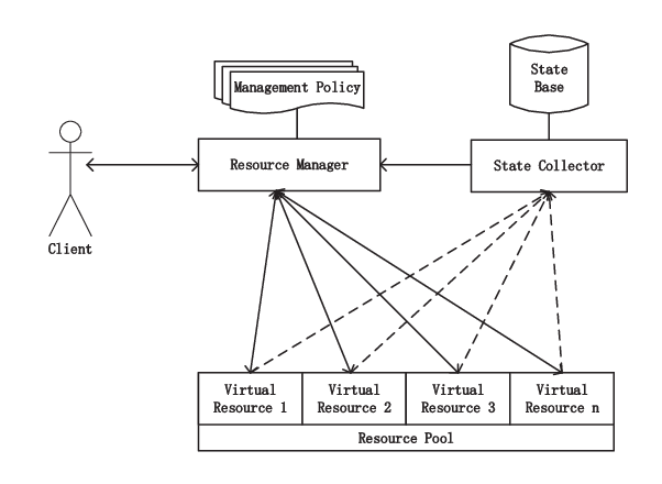
Refer to caption
Figure 6: An architecture of cloud resource management

As shown in Figure 6, the typical execution process of cloud resource management is as follows.

  1. 1.

    The Client receives the resource accessing requests, and sends them to the Resource manager;

  2. 2.

    The Resource Manager receives the requests from the Client, divides the computational tasks, creates the related virtual resources, and sends the divided tasks to the involved virtual resources;

  3. 3.

    The created virtual resources receives their tasks from the Resource Manager, accesses the actual resources to run the computational tasks, during the running, they report their running states to State Collector;

  4. 4.

    The State Collector receives the running states from the virtual resources, store the states into the State Base, and sends the running states of the involved virtual resources to the Resource Manager;

  5. 5.

    The Resource Manager receives the running states, after an inner processing, sends the states to the Client;

  6. 6.

    The Client receives the states and sends them to the outside;

  7. 7.

    When the running of virtual resources are finished, they sends the results to the Resource Manager;

  8. 8.

    The Resource Manager receives the computational results, after an inner combination, sends the combined results to the Client;

  9. 9.

    The Client receives the results and sends them to the outside.

6.2 The New Actor Model of Cloud Resource Management

According to the architecture of cloud resource management, the whole actors system implemented by actors can be divided into four kinds of actors: the client actor (CA), the Virtual Resource actors (VAs), the Resource Manager actor (RA) and the State Collector actor (SA).

6.2.1 Client Actor, CA

We use an actor called Client actor (CA) to model the Client.

After the CA is created, the typical process is as follows.

  1. 1.

    The CA receives the requests D​IC​ADI_{CA} from the outside through its mail box denoted by its name C​ACA (the corresponding reading action is denoted rC​A​(D​IC​A)r_{CA}(DI_{CA}));

  2. 2.

    Then it does some local computations mixed some atomic actions by computation logics, including ⋅\cdot, ++, ≬\between and guards, the whole local computations are denoted and included into IC​AI_{CA}, which is the set of all local atomic actions;

  3. 3.

    When the local computations are finished, the CA generates the output requests D​IR​ADI_{RA}, and sends to the RA’s mail box denoted by the RA’s name R​ARA (the corresponding sending action is denoted sR​A​(D​IR​A)s_{RA}(DI_{RA}));

  4. 4.

    The CA receives the running states (we assume just one time) from RA through its mail box denoted by its name C​ACA (the corresponding reading actions are denoted rC​A​(R​SR​A)r_{CA}(RS_{RA}));

  5. 5.

    Then it does some local computations mixed some atomic actions by computation logics, including ⋅\cdot, ++, ≬\between and guards, the whole local computations are denoted and included into IC​AI_{CA}, which is the set of all local atomic actions;

  6. 6.

    When the local computations are finished, the CA generates the output states R​SC​ARS_{CA} (containing the files), and sends to the outside (the corresponding sending action is denoted sO​(R​SC​A)s_{O}(RS_{CA}));

  7. 7.

    The CA receives the computational results from RA through its mail box denoted by its name C​ACA (the corresponding reading actions are denoted rC​A​(C​RR​A)r_{CA}(CR_{RA}));

  8. 8.

    Then it does some local computations mixed some atomic actions by computation logics, including ⋅\cdot, ++, ≬\between and guards, the whole local computations are denoted and included into IC​AI_{CA}, which is the set of all local atomic actions;

  9. 9.

    When the local computations are finished, the CA generates the output message D​OC​ADO_{CA}, and sends to the outside (the corresponding sending action is denoted sO​(D​OC​A)s_{O}(DO_{CA})), and then processes the next message from the outside recursively.

The above process is described as the following state transitions by APTC.

C​A=rC​A​(D​IC​A)⋅C​A1CA=r_{CA}(DI_{CA})\cdot CA_{1}

C​A1=IC​A⋅C​A2CA_{1}=I_{CA}\cdot CA_{2}

C​A2=sR​A​(D​IR​A)⋅C​A3CA_{2}=s_{RA}(DI_{RA})\cdot CA_{3}

C​A3=rC​A​(R​SR​A)⋅C​A4CA_{3}=r_{CA}(RS_{RA})\cdot CA_{4}

C​A4=IC​A⋅C​A5CA_{4}=I_{CA}\cdot CA_{5}

C​A5=sO​(R​SC​A)⋅C​A6CA_{5}=s_{O}(RS_{CA})\cdot CA_{6}

C​A6=rC​A​(C​RR​A)⋅C​A7CA_{6}=r_{CA}(CR_{RA})\cdot CA_{7}

C​A7=IC​A⋅C​A8CA_{7}=I_{CA}\cdot CA_{8}

C​A8=sO​(D​OC​A)⋅C​ACA_{8}=s_{O}(DO_{CA})\cdot CA

By use of the algebraic laws of APTC, the CA may be proven exhibiting desired external behaviors. If it can exhibits desired external behaviors, the CA should have the following form:

τIC​A​(∂∅(C​A))=rC​A​(D​IC​A)⋅sR​A​(D​IR​A)⋅rC​A​(R​SR​A)⋅sO​(R​SC​A)⋅rC​A​(C​RR​A)⋅sO​(D​OC​A)⋅τIC​A​(∂∅(C​A))\tau_{I_{CA}}(\partial_{\emptyset}(CA))=r_{CA}(DI_{CA})\cdot s_{RA}(DI_{RA})\cdot r_{CA}(RS_{RA})\cdot s_{O}(RS_{CA})\cdot r_{CA}(CR_{RA})\\ \cdot s_{O}(DO_{CA})\cdot\tau_{I_{CA}}(\partial_{\emptyset}(CA))

6.2.2 Virtual Resource Actor, VA

A Virtual Resource is an atomic function unit to access actual resource and managed by the RA. We use an actor called Virtual Resource actor (VA) to model a Virtual Resource.

A VA has a unique name, local information and variables to contain its states, and local computation procedures to manipulate the information and variables. A VA is always managed by the Master and it receives messages from the Master, sends messages to the Master and the client, and is created by the Master. Note that a VA can not create new VAs, it can only be created by the Master. That is, a VA is an actor with a constraint that is without create action.

After a VA is created, the typical process is as follows.

  1. 1.

    The VA receives the computational tasks D​IV​ADI_{VA} from RA through its mail box denoted by its name V​AVA (the corresponding reading action is denoted rV​A​(D​IV​A)r_{VA}(DI_{VA}));

  2. 2.

    Then it does some local computations mixed some atomic actions by computation logics, including ⋅\cdot, ++, ≬\between and guards, the whole local computations are denoted and included into IV​AI_{VA}, which is the set of all local atomic actions;

  3. 3.

    During the local computations, generates the running states R​SV​ARS_{VA}, and sends them (we assume just one time) to the SA’s mail box denoted by the SA’s name S​ASA (the corresponding sending action is denoted sS​A​(R​SV​A)s_{SA}(RS_{VA}));

  4. 4.

    Then it does some local computations mixed some atomic actions by computation logics, including ⋅\cdot, ++, ≬\between and guards, the whole local computations are denoted and included into IV​AI_{VA}, which is the set of all local atomic actions;

  5. 5.

    If the local computations are finished, VA generates the computational results C​RV​ACR_{VA}, and sends them to the RA’s mail box denoted by the RA’s name R​ARA (the corresponding sending action is denoted sR​A​(C​RV​A)s_{RA}(CR_{VA})), and then processes the next task from RA recursively.

The above process is described as the following state transitions by APTC.

V​A=rV​A​(D​IV​A)⋅V​A1VA=r_{VA}(DI_{VA})\cdot VA_{1}

V​A1=IV​A⋅V​A2VA_{1}=I_{VA}\cdot VA_{2}

V​A2=sS​A​(R​SV​A)⋅V​A3VA_{2}=s_{SA}(RS_{VA})\cdot VA_{3}

V​A3=IV​A⋅V​A4VA_{3}=I_{VA}\cdot VA_{4}

V​A4=sR​A​(C​RV​A)⋅V​AVA_{4}=s_{RA}(CR_{VA})\cdot VA

By use of the algebraic laws of APTC, the VA may be proven exhibiting desired external behaviors. If it can exhibits desired external behaviors, the VA should have the following form:

τIV​A​(∂∅(V​A))=rV​A​(D​IV​A)⋅sS​A​(R​SV​A)⋅sR​A​(C​RV​A)⋅τIV​A​(∂∅(V​A))\tau_{I_{VA}}(\partial_{\emptyset}(VA))=r_{VA}(DI_{VA})\cdot s_{SA}(RS_{VA})\cdot s_{RA}(CR_{VA})\cdot\tau_{I_{VA}}(\partial_{\emptyset}(VA))

6.2.3 Resource Manager Actor, RA

RA receives the requests from the client, and manages the VAs. We use an actor called Resource Manager actor (RA) to model the Resource Manager.

After RA is created, the typical process is as follows.

  1. 1.

    The RA receives the requests D​IR​ADI_{RA} from the Client through its mail box denoted by its name R​ARA (the corresponding reading action is denoted rR​A​(D​IR​A)r_{RA}(DI_{RA}));

  2. 2.

    Then it does some local computations mixed some atomic actions by computation logics, including ⋅\cdot, ++, ≬\between and guards, the whole local computations are denoted and included into IR​AI_{RA}, which is the set of all local atomic actions;

  3. 3.

    The RA creates nn VAs V​AiVA_{i} for 1≤i≤n1\leq i\leq n in parallel through actions 𝐧𝐞𝐰⁡(V​A1)|⋯|𝐧𝐞𝐰⁡(V​An)\mathbf{new}(VA_{1})\parallel\cdots\parallel\mathbf{new}(VA_{n});

  4. 4.

    When the local computations are finished, the RA generates the computational tasks D​IV​AiDI_{VA_{i}} for each V​AiVA_{i} with 1≤i≤n1\leq i\leq n, sends them to the VAs’ mail box denoted by the VAs’ name V​AiVA_{i} (the corresponding sending actions are denoted sV​A1​(D​IV​A1)|⋯|sV​An​(D​IV​An)s_{VA_{1}}(DI_{VA_{1}})\parallel\cdots\parallel s_{VA_{n}}(DI_{VA_{n}}));

  5. 5.

    The RA receives the running states R​SS​ARS_{SA} (we assume just one time) from the SA through its mail box denoted by its name R​ARA (the corresponding reading action is denoted rR​A​(R​SS​A)r_{RA}(RS_{SA}));

  6. 6.

    Then it does some local computations mixed some atomic actions by computation logics, including ⋅\cdot, ++, ≬\between and guards, the whole local computations are denoted and included into IR​AI_{RA}, which is the set of all local atomic actions;

  7. 7.

    When the local computations are finished, the RA generates running states R​SR​ARS_{RA}, sends them to the CAs’ mail box denoted by the CAs’ name C​ACA (the corresponding sending actions are denoted sC​A​(R​SR​A)s_{CA}(RS_{RA}));

  8. 8.

    The RA receives the computational results C​RV​AiCR_{VA_{i}} from the V​AiVA_{i} for 1≤i≤n1\leq i\leq n through its mail box denoted by its name R​ARA (the corresponding reading action is denoted rR​A​(C​RV​A1)|⋯|rR​A​(C​RV​An)r_{RA}(CR_{VA_{1}})\parallel\cdots\parallel r_{RA}(CR_{VA_{n}}));

  9. 9.

    Then it does some local computations mixed some atomic actions by computation logics, including ⋅\cdot, ++, ≬\between and guards, the whole local computations are denoted and included into IR​AI_{RA}, which is the set of all local atomic actions;

  10. 10.

    When the local computations are finished, the RA generates results C​RR​ACR_{RA}, sends them to the CAs’ mail box denoted by the CAs’ name C​ACA (the corresponding sending actions are denoted sC​A​(C​RR​A)s_{CA}(CR_{RA})), and then processes the next message from the client recursively.

The above process is described as the following state transitions by APTC.

R​A=rR​A​(D​IR​A)⋅R​A1RA=r_{RA}(DI_{RA})\cdot RA_{1}

R​A1=IR​A⋅R​A2RA_{1}=I_{RA}\cdot RA_{2}

R​A2=𝐧𝐞𝐰⁡(V​A1)|⋯|𝐧𝐞𝐰⁡(V​An)⋅R​A3RA_{2}=\mathbf{new}(VA_{1})\parallel\cdots\parallel\mathbf{new}(VA_{n})\cdot RA_{3}

R​A3=sV​A1​(D​IV​A1)|⋯|sV​An​(D​IV​An)⋅R​A4RA_{3}=s_{VA_{1}}(DI_{VA_{1}})\parallel\cdots\parallel s_{VA_{n}}(DI_{VA_{n}})\cdot RA_{4}

R​A4=rR​A​(R​SS​A)⋅R​A5RA_{4}=r_{RA}(RS_{SA})\cdot RA_{5}

R​A5=IR​A⋅R​A6RA_{5}=I_{RA}\cdot RA_{6}

R​A6=sC​A​(R​SR​A)⋅R​A7RA_{6}=s_{CA}(RS_{RA})\cdot RA_{7}

R​A7=rR​A​(C​RV​A1)|⋯|rR​A​(C​RV​An)⋅R​A8RA_{7}=r_{RA}(CR_{VA_{1}})\parallel\cdots\parallel r_{RA}(CR_{VA_{n}})\cdot RA_{8}

R​A8=IR​A⋅R​A9RA_{8}=I_{RA}\cdot RA_{9}

R​A9=sC​A​(C​RR​A)⋅R​ARA_{9}=s_{CA}(CR_{RA})\cdot RA

By use of the algebraic laws of APTC, the RA may be proven exhibiting desired external behaviors. If it can exhibits desired external behaviors, the RA should have the following form:

τIR​A(∂∅(RA))=rR​A(DIR​A)⋅(sV​A1(DIV​A1)∥⋯∥sV​An(DIV​An))⋅rR​A(RSS​A)⋅sC​A(RSR​A)⋅(rR​A(CRV​A1)∥⋯∥rR​A(CRV​An))⋅sC​A(CRR​A)⋅τIR​A(∂∅(RA))\tau_{I_{RA}}(\partial_{\emptyset}(RA))=r_{RA}(DI_{RA})\cdot(s_{VA_{1}}(DI_{VA_{1}})\parallel\cdots\parallel s_{VA_{n}}(DI_{VA_{n}}))\cdot\\ r_{RA}(RS_{SA})\cdot s_{CA}(RS_{RA})\cdot(r_{RA}(CR_{VA_{1}})\parallel\cdots\parallel r_{RA}(CR_{VA_{n}}))\cdot s_{CA}(CR_{RA})\cdot\tau_{I_{RA}}(\partial_{\emptyset}(RA))

6.2.4 State Collector Actor, SA

We use an actor called State Collector actor (SA) to model the State Collector.

After the SA is created, the typical process is as follows.

  1. 1.

    The SA receives the running states R​SV​AiRS_{VA_{i}} from V​AiVA_{i} (we assume just one time) for 1≤i≤n1\leq i\leq n through its mail box denoted by its name S​ASA (the corresponding reading action is denoted rS​A​(R​SV​A1)|⋯|rS​A​(R​SV​An)r_{SA}(RS_{VA_{1}})\parallel\cdots\parallel r_{SA}(RS_{VA_{n}}));

  2. 2.

    Then it does some local computations mixed some atomic actions by computation logics, including ⋅\cdot, ++, ≬\between and guards, the whole local computations are denoted and included into IS​AI_{SA}, which is the set of all local atomic actions;

  3. 3.

    When the local computations are finished, SA generates the running states R​SS​ARS_{SA}, and sends them to the RA’s mail box denoted by the RA’s name R​ARA (the corresponding sending action is denoted sR​A​(R​SS​A)s_{RA}(RS_{SA})), and then processes the next task from RA recursively.

The above process is described as the following state transitions by APTC.

S​A=rS​A​(R​SV​A1)|⋯|rS​A​(R​SV​An)⋅S​A1SA=r_{SA}(RS_{VA_{1}})\parallel\cdots\parallel r_{SA}(RS_{VA_{n}})\cdot SA_{1}

S​A1=IS​A⋅S​A2SA_{1}=I_{SA}\cdot SA_{2}

S​A2=sR​A​(R​SS​A)⋅S​ASA_{2}=s_{RA}(RS_{SA})\cdot SA

By use of the algebraic laws of APTC, the SA may be proven exhibiting desired external behaviors. If it can exhibits desired external behaviors, the SA should have the following form:

τIS​A(∂∅(SA))=(rS​A(RSV​A1)∥⋯∥rS​A(RSV​An))⋅sR​A(RSS​A))⋅τIS​A(∂∅(SA))\tau_{I_{SA}}(\partial_{\emptyset}(SA))=(r_{SA}(RS_{VA_{1}})\parallel\cdots\parallel r_{SA}(RS_{VA_{n}}))\cdot s_{RA}(RS_{SA}))\cdot\tau_{I_{SA}}(\partial_{\emptyset}(SA))

6.2.5 Putting All Together into A Whole

We put all actors together into a whole, including all CA, VAs, RA and SA, according to the architecture as illustrated in Figure 6. The whole actor system C​AR​AS​A=C​AR​AS​AV​A1⋯V​AnCA\quad RA\quad SA=CA\quad RA\quad SA\quad\\ VA_{1}\quad\cdots\quad VA_{n} can be represented by the following process term of APTC.

τI​(∂H(C​A≬R​A≬S​A))=τI​(∂H(C​A≬R​A≬S​A≬V​A1≬⋯≬V​An))\tau_{I}(\partial_{H}(CA\between RA\between SA))=\tau_{I}(\partial_{H}(CA\between RA\between SA\between VA_{1}\between\cdots\between VA_{n}))

Among all the actors, there are synchronous communications. The actor’s reading and to the same actor’s sending actions with the same type messages may cause communications. If to the actor’s sending action occurs before the the same actions reading action, an asynchronous communication will occur; otherwise, a deadlock δ\delta will be caused.

There are four kinds of asynchronous communications as follows.

(1) The communications between a VA and RA with the following constraints.

sV​A​(D​IV​A)≤rV​A​(D​IV​A)s_{VA}(DI_{VA})\leq r_{VA}(DI_{VA})

sR​A​(C​RV​A)≤rR​A​(C​RV​A)s_{RA}(CR_{VA})\leq r_{RA}(CR_{VA})

(2) The communications between a VA and SA with the following constraints.

sS​A​(R​SV​A)≤rS​A​(R​SV​A)s_{SA}(RS_{VA})\leq r_{SA}(RS_{VA})

(3) The communications between CA and RA with the following constraints.

sR​A​(D​IR​A)≤rR​A​(D​IR​A)s_{RA}(DI_{RA})\leq r_{RA}(DI_{RA})

sC​A​(R​SR​A)≤rC​A​(R​SR​A)s_{CA}(RS_{RA})\leq r_{CA}(RS_{RA})

sC​A​(C​RR​A)≤rC​A​(C​RR​A)s_{CA}(CR_{RA})\leq r_{CA}(CR_{RA})

(4) The communications between RA and SA with the following constraints.

sR​A​(R​SS​A)≤rR​A​(R​SS​A)s_{RA}(RS_{SA})\leq r_{RA}(RS_{SA})

So, the set HH and II can be defined as follows.

H={sV​A1(DIV​A1),rV​A1(DIV​A1),⋯,sV​An(DIV​An),rV​An(DIV​An),sR​A(CRV​A1),rR​A(CRV​A1),⋯,sR​A(CRV​An),rR​A(CRV​An),sS​A(RSV​A1),rS​A(RSV​A1),⋯,sS​A(RSV​An),rS​A(RSV​An),sR​A(DIR​A),rR​A(DIR​A),sC​A(RSR​A),rC​A(RSR​A),sC​A(CRR​A),rC​A(CRR​A),sR​A(RSS​A),rR​A(RSS​A)|sV​A1(DIV​A1)≰rV​A1(DIV​A1),⋯,sV​An(DIV​An)≰rV​An(DIV​An),sR​A(CRV​A1)≰rR​A(CRV​A1),⋯,sR​A(CRV​An)≰rR​A(CRV​An),sS​A(RSV​A1)≰rS​A(RSV​A1),⋯,sS​A(RSV​An)≰rS​A(RSV​An),sR​A(DIR​A)≰rR​A(DIR​A),sC​A(RSR​A)≰rC​A(RSR​A),sC​A(CRR​A)≰rC​A(CRR​A),sR​A(RSS​A)≰rR​A(RSS​A)}H=\{s_{VA_{1}}(DI_{VA_{1}}),r_{VA_{1}}(DI_{VA_{1}}),\cdots,s_{VA_{n}}(DI_{VA_{n}}),r_{VA_{n}}(DI_{VA_{n}}),\\ s_{RA}(CR_{VA_{1}}),r_{RA}(CR_{VA_{1}}),\cdots,s_{RA}(CR_{VA_{n}}),r_{RA}(CR_{VA_{n}}),\\ s_{SA}(RS_{VA_{1}}),r_{SA}(RS_{VA_{1}}),\cdots,s_{SA}(RS_{VA_{n}}),r_{SA}(RS_{VA_{n}}),\\ s_{RA}(DI_{RA}),r_{RA}(DI_{RA}),s_{CA}(RS_{RA}),r_{CA}(RS_{RA}),\\ s_{CA}(CR_{RA}),r_{CA}(CR_{RA}),s_{RA}(RS_{SA}),r_{RA}(RS_{SA})\\ |s_{VA_{1}}(DI_{VA_{1}})\nleq r_{VA_{1}}(DI_{VA_{1}}),\cdots,s_{VA_{n}}(DI_{VA_{n}})\nleq r_{VA_{n}}(DI_{VA_{n}}),\\ s_{RA}(CR_{VA_{1}})\nleq r_{RA}(CR_{VA_{1}}),\cdots,s_{RA}(CR_{VA_{n}})\nleq r_{RA}(CR_{VA_{n}}),\\ s_{SA}(RS_{VA_{1}})\nleq r_{SA}(RS_{VA_{1}}),\cdots,s_{SA}(RS_{VA_{n}})\nleq r_{SA}(RS_{VA_{n}}),\\ s_{RA}(DI_{RA})\nleq r_{RA}(DI_{RA}),s_{CA}(RS_{RA})\nleq r_{CA}(RS_{RA}),\\ s_{CA}(CR_{RA})\nleq r_{CA}(CR_{RA}),s_{RA}(RS_{SA})\nleq r_{RA}(RS_{SA})\}

I={sV​A1(DIV​A1),rV​A1(DIV​A1),⋯,sV​An(DIV​An),rV​An(DIV​An),sR​A(CRV​A1),rR​A(CRV​A1),⋯,sR​A(CRV​An),rR​A(CRV​An),sS​A(RSV​A1),rS​A(RSV​A1),⋯,sS​A(RSV​An),rS​A(RSV​An),sR​A(DIR​A),rR​A(DIR​A),sC​A(RSR​A),rC​A(RSR​A),sC​A(CRR​A),rC​A(CRR​A),sR​A(RSS​A),rR​A(RSS​A)|sV​A1(DIV​A1)≤rV​A1(DIV​A1),⋯,sV​An(DIV​An)≤rV​An(DIV​An),sR​A(CRV​A1)≤rR​A(CRV​A1),⋯,sR​A(CRV​An)≤rR​A(CRV​An),sS​A(RSV​A1)≤rS​A(RSV​A1),⋯,sS​A(RSV​An)≤rS​A(RSV​An),sR​A(DIR​A)≤rR​A(DIR​A),sC​A(RSR​A)≤rC​A(RSR​A),sC​A(CRR​A)≤rC​A(CRR​A),sR​A(RSS​A)≤rR​A(RSS​A)}∪IC​A∪IV​A1∪⋯∪IV​An∪IR​A∪IS​AI=\{s_{VA_{1}}(DI_{VA_{1}}),r_{VA_{1}}(DI_{VA_{1}}),\cdots,s_{VA_{n}}(DI_{VA_{n}}),r_{VA_{n}}(DI_{VA_{n}}),\\ s_{RA}(CR_{VA_{1}}),r_{RA}(CR_{VA_{1}}),\cdots,s_{RA}(CR_{VA_{n}}),r_{RA}(CR_{VA_{n}}),\\ s_{SA}(RS_{VA_{1}}),r_{SA}(RS_{VA_{1}}),\cdots,s_{SA}(RS_{VA_{n}}),r_{SA}(RS_{VA_{n}}),\\ s_{RA}(DI_{RA}),r_{RA}(DI_{RA}),s_{CA}(RS_{RA}),r_{CA}(RS_{RA}),\\ s_{CA}(CR_{RA}),r_{CA}(CR_{RA}),s_{RA}(RS_{SA}),r_{RA}(RS_{SA})\\ |s_{VA_{1}}(DI_{VA_{1}})\leq r_{VA_{1}}(DI_{VA_{1}}),\cdots,s_{VA_{n}}(DI_{VA_{n}})\leq r_{VA_{n}}(DI_{VA_{n}}),\\ s_{RA}(CR_{VA_{1}})\leq r_{RA}(CR_{VA_{1}}),\cdots,s_{RA}(CR_{VA_{n}})\leq r_{RA}(CR_{VA_{n}}),\\ s_{SA}(RS_{VA_{1}})\leq r_{SA}(RS_{VA_{1}}),\cdots,s_{SA}(RS_{VA_{n}})\leq r_{SA}(RS_{VA_{n}}),\\ s_{RA}(DI_{RA})\leq r_{RA}(DI_{RA}),s_{CA}(RS_{RA})\leq r_{CA}(RS_{RA}),\\ s_{CA}(CR_{RA})\leq r_{CA}(CR_{RA}),s_{RA}(RS_{SA})\leq r_{RA}(RS_{SA})\}\\ \cup I_{CA}\cup I_{VA_{1}}\cup\cdots\cup I_{VA_{n}}\cup I_{RA}\cup I_{SA}

Then, we can get the following conclusion.

Theorem 6.1.

The whole actor system of cloud resource management illustrated in Figure 6 can exhibits desired external behaviors.

Proof.

By use of the algebraic laws of APTC, we can prove the following equation:

τI​(∂H(C​A≬R​A≬S​A))=τI​(∂H(C​A≬R​A≬S​A≬V​A1≬⋯≬V​An))=rC​A​(D​IC​A)⋅sO​(R​SC​A)⋅sO​(C​RC​A)⋅τI​(∂H(C​A≬R​A≬S​A≬V​A1≬⋯≬V​An))=rC​A​(D​IC​A)⋅sO​(R​SC​A)⋅sO​(C​RC​A)⋅τI​(∂H(C​A≬R​A≬S​A))\tau_{I}(\partial_{H}(CA\between RA\between SA))=\tau_{I}(\partial_{H}(CA\between RA\between SA\between VA_{1}\between\cdots\between VA_{n}))\\ =r_{CA}(DI_{CA})\cdot s_{O}(RS_{CA})\cdot s_{O}(CR_{CA})\cdot\tau_{I}(\partial_{H}(CA\between RA\between SA\between VA_{1}\between\cdots\between VA_{n}))\\ =r_{CA}(DI_{CA})\cdot s_{O}(RS_{CA})\cdot s_{O}(CR_{CA})\cdot\tau_{I}(\partial_{H}(CA\between RA\between SA))

For the details of the proof, we omit them, please refer to section 2.10. ∎

7 Process Algebra Based Actor Model of Web Service Composition

In this chapter, we will use the process algebra based actor model to model and verify Web Service composition based on the previous work [20]. In section 7.1, we introduce the requirements of Web Service composition runtime system; we model the Web Service composition runtime by use of the new actor model in section 7.2; finally, we take an example to show the usage of the model in section 7.3.

7.1 Requirements of Web Service Composition

Web Service (WS) is a distributed software component which emerged about ten years ago to utilize the most widely-used Internet application protocol–HTTP as its base transport protocol. As a component, a WS has the similar ingredients as other ones, such as DCOM, EJB, CORBA, and so on. That is, a WS uses HTTP-based SOAP as its transport protocol, WSDL as its interface description language and UDDI as its name and directory service.

WS Composition creates new composite WSs using different composition patterns from the collection of existing WSs. Because of advantages of WS to solve cross-organizational application integrations, two composition patterns are dominant. One is called Web Service Orchestration (WSO) [18], which uses a workflow-like composition pattern to orchestrate business activities (implemented as WS Operations) and models a cross-organizational business processes or other kind of processes. The other is called Web Service Choreography (WSC) [19] which has an aggregate composition pattern to capture the external interaction behaviors of WSs and acts as a contract or a protocol among WSs.

We now take a simple example of buying books from a book store to illustrate some concepts of WS composition. Though this example is quite simple and only includes the sequence control flow (that is, each business activity in a business process is executed in sequence), it is enough to explain the concepts and ideas of this paper and avoids unnecessary complexity without loss of generality. We use this example throughout this paper. The requirements of this example are as Figure 7 shows.
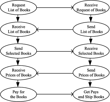
Refer to caption
Figure 7: Requirements of an example

A customer buys books from a book store through a user agent. In this example, we ignore interactions between the customer and the user agent, and focus on those between the user agent and the book store. Either user agent or book store has business processes to interact with each other.

We give the process of user agent as follows. The process of book store can be gotten from that of user agent as contrasts.

  1. 1.

    The user agent requests a list of all books to the book store;

  2. 2.

    It gets the book list from the book store;

  3. 3.

    It selects the books by the customer and sends the list of selected books to the book store;

  4. 4.

    It receives the prices of selected books from the book store;

  5. 5.

    It accepts the prices and pays for the selected book to the book store. Then the process terminates.

Since the business activities, such as the book store accepting request for a list of books from the user agent, are implemented as WSs (exactly WS operations), such buyer agent and book store business processes are called WSOs. These WSOs are published as WSs called their interface WSs for interacting among each other. The interaction behaviors among WSs described by some contracts or protocols are called WSCs.

There are many efforts for WS Composition, including its specifications, design methods and verifications, simulations, and runtime supports. Different methods and tools are used in WS Composition research, such as XML-based WSO description specifications and WSC description specifications, formal verification techniques based on Process Algebra and Petri-Net, and runtime implementations using programming languages. Some of these works mainly focus on WSO, others mainly on WSC, and also a few works attempt to establish a relationship between WSO and WSC.

Can a WS interact with another one? And also, can a WSO interact with another one via their interfaces? Is the definition of a WSC compatible with its partner WSs or partner WSOs? To solve these problems, a correct relationship between WSO and WSC must be established. A WS Composition system combining WSO and WSC, with a natural relationship between the two ones, is an attractive direction. In a systematic viewpoint, WS, WSO and WSC are organized with a natural relationship under the whole environment of cross-organizational business integration. More importantly, such a system should have firmly theoretic foundation.

In this chapter, we try to make such a system to base on the new actor model.

7.1.1 WSO and WSC

A WS is a distributed software component with transport protocol–SOAP, interface description by WSDL, and can be registered into UDDI to be searched and discovered by its customers.

A WSO orchestrates WSs existing on the Web into a process through the so-called control flow constructs. That is, within a WSO, there are a collection of atomic function units called activities with control flows to manipulate them. So, the main ingredients of a WSO are following.

  • •

    Inputs and Outputs: At the start time of a WSO, it accepts some inputs. And it sends out outcomes at the end of its execution;

  • •

    Information and Variable Definitions: A WSO has local states which maybe transfer among activities. Finally, the local states are sent to WSs outside by activities in the form of messages. In turn, activities receiving message outside can alter the local states;

  • •

    Activity Definitions: An activity is an atomic unit with several pre-defined function kinds, such as invoking a WS outside, invoking an application inside, receiving a request from a customer inside/outside, local variable assignments, etc;

  • •

    Control Flow Definitions: Control flow definitions give activities an execution order. In terms of structural model based control flow definitions, control flows are the so-called structural activities which can be sequence activity, choice activity, loop activity, parallel activity and their variants;

  • •

    Binding WS Information: Added values of WS Composition are the so called recursive composition, that is, a WSO orchestrating existing WSs is published as a new WS itself too. A WSO interacts with other WSs outside through this new WS.

In Figure 7, the user agent business process is modeled as UserAgent WSO described by WS-BPEL, which is described in Appendix A.

The interface WS for UserAgent WSO is called UserAgent WS described by WSDL, which also can be found in Appendix A.

A WSC defines the external interaction behaviors and serves as a contract or a protocol among WSs. The main ingredients of a WSC are as following.

  • •

    Parter Definitions: They defines the partners within a WSC including the role of a partner acting as and relationships among partners;

  • •

    Information and Variable Definitions: A WSC may also have local states exchanged among the interacting WSs;

  • •

    Interactions among Partners: Interaction points and interaction behaviors are defined as the core contents in a WSC.

In the buying books example, the WSC between user agent and bookstore (exactly UserAgentWS and BookStoreWS) called BuyingBookWSC is described by WS-CDL, which can be found in Appendix A.

The WSO and the WSC define two different aspects of WS Composition. Their relationships as Figure 8 illustrates. Note that a WSO may require at least a WSC, but a WSC does not need to depend on a WSO.

Refer to caption
Figure 8: Relationship between WSO and WSC

7.1.2 Design Decisions on Web Service Composition Runtime

(1) Stateless WS or Stateful WS

In the viewpoint of W3C, a WS itself is an interface or a wrapper of an application inside the boundary of an organization that has a willing to interact with applications outside. That is, a W3C WS has no an independent programming model like other component models and has no needs of containing local states for local computations. Indeed, there are different sounds of developing WS to be a full sense component, Such as OGSI. Incompatibility between W3C WS and OGSI-like WS leads to WSRF as a compromised solution which reserves the W3C WS and develops a notion of WS Resource to model states.

We adopt the ideas of WSRF. That is, let WS be an interface or a wrapper of WSO and let WSO be a special kind WS Resource which has local states and local computations. The interface WS of a WSO reserves ID of the WSO to deliver an incoming message to the WSO and send an outgoing message with the ID attached in order for delivering a call-back message. Further more, a WSO and its WS are one-one binding. When a new incoming message arrives without a WSO ID attached, the WS creates a new WSO and attaches its ID as a parameter.

(2) Incoming Messages and Outgoing Messages

Just as the name implies, a WS serves as a server to process an incoming message within a C/S framework. But an interaction between a component WS or a WSO requires incoming message and outgoing message pairs. When an interaction occurred, one serves as a client and the other serves as a server. But in the next interaction, the one served as client before may serve as a server and the server becomes a client.

The problem is that, when a WSO (or other kind WS Resource) inside interacts with WSs outside, who is willing to act as the bridge between the WSO inside and WSs outside? When an incoming message arrives, it is easily to be understood that the incoming message is delivered to the WSO by the interface WS. However, how is an outgoing message from a WSO inside to a component WS outside delivered?

In fact, there are two ways to solve the outgoing message. One is the way of WS-BPEL [18], and the other is that of an early version of WSDL. The former uses a so-called invoke atomic activity defined in a WSO to send an outgoing message directly without the assistant of its interface WS. In contrast, the latter specifies that every thing exchanged between resources inside and functions outside must go via the interface WS of the resource inside. Furthermore, in an early edition of WSDL, there are four kind of WS operations are defined, including an In operation, an In-Out operation, an Out operation and an Out-In operation. In operation and In-Out operation receive the incoming messages, while Out operation and Out-In operation deliver the outgoing messages. Out operation and Out-In operation are somewhat strange because a WS is a kind of server in nature. So, in the later versions of WSDL, Out operation and Out-In operation are removed. But the problem of how to process the outgoing message is remaining.

The way of WS-BPEL will cause some confusions in the WS Composition runtime architecture design. And the way of the early edition of WSDL looks somewhat strange. So, our way of processing outgoing message is a compromise of the above two ones. That is, the outgoing messages from an internal WSO to an external resource, must go via the WS of the internal WSO. But the WS does not need to declare operations for processing the outgoing messages in the WSDL definitions.

(3) Functions and Enablements of WSC

A WSC acts as a contract or a protocol between interacting WSs. In a viewpoint of business integration requirements, a WSC serves as a business contract to constrain the rights and obligations of business partners. And from a view of utilized technologies, a WSC can be deemed as a communication protocol which coordinates the interaction behaviors of involved WSs.

About the enablements of a WSC, there are also two differently enable patterns. One is a concentrated architecture and the the other is a distributed one.

The concentrated way considers that the enablements of a WSC must be under supervision of a thirdly authorized party or all involved partners. An absolutely concentrated way maybe require that any operation about interacting WSs must be done by the way of a supervisor. This way maybe cause the supervisor becoming a performance bottleneck when bulk of interactions occur, but it can bring trustworthiness of interaction results if the supervisor is trustworthy itself.

The distributed way argues that each WS interacts among others with constraints of a WSC and there is no need of a supervisor. It is regarded that WSs just behave correctly to obey to a WSC and maybe take an example of enablements of open Internet protocols. But there are cheating business behaviors of an intendedly incorrect WS, that are unlike almost purely technical motivations of open Internet protocols.

We use a hybrid enablements of WSC. That is, when a WSC is contracted (either contracted dynamically at runtime or contracted with human interventions at design time) among WSs and enabled, the WSC creates the partner WSs at the beginning of enablements. And then the WSs interact with each other.

7.1.3 A WS Composition Runtime Architecture

Based on the above introductions and discussions, we design an architecture of WS Composition runtime as Figure 9 shows. Figure 9 illustrates the typical architecture of a WS Composition runtime. We explain the compositions and their relationships in the following. There are four components: WSO, WS, WSC and applications inside.

Refer to caption
Figure 9: An architecture of WS composition runtime

The functions and ingredients of a WSO usually it have a collection of activities that may interact with partner WSs outside or applications inside. Enablements of a WSO require a runtime environment which is not illustrated in Figure 9. For examples, execution of a WSO described by WS-BPEL needs a WS-BPEL interpreter (also called WSO engine). A WSO locates in the interior of an organization. It interacts with applications inside with private exchanging mechanisms and with other partner WSOs outside via its interface WS.

Applications inside may be any legacy application or any newly developed application within the interior of a organization. These applications can be implemented in any technical framework and provide interfaces to interact with other applications inside, including a WSO. Interactions between a WSO and a application inside may base on any private communication mechanism, such as local object method call, RPC, RMI, etc, which depends on technical framework adopted by the application.

An interface WS acts as an interface of a WSO to interact with partner WSs outside. A WSO is with an one-to-one binding to its interface WS and is created by its interface WS at the time of first interaction with exterior. Enablements of a WS also require a runtime support usually called SOAP engine which implies a HTTP server installed to couple with HTTP requests. A WS and its runtime support locate at demilitarized zone (DMZ) of an organization which has different management policies and different security policies to the interior of an organization.

A WSC acts as a contract or a protocol of partner WSs. When a WSC is enabled, it creates all partner WSs at their accurate positions. Enablements of a WSC also require a runtime support to interpret the WSC description language like WS-CDL. A WSC and its support environment can be located at a thirdly authorized party or other places negotiated by the partners.

7.2 The New Actor Model of Web Service Composition

According to the architecture of WS composition runtime, the whole actors system implemented by actors can be divided into four kinds of actors: the activity actors, the WS actors, the WSO actors and the WSC actor.

7.2.1 Activity Actor, AA

An activity is an atomic function unit of a WSO and is managed by the WSO. We use an actor called activity actor (AA) to model an activity.

An AA has a unique name, local information and variables to contain its states, and local computation procedures to manipulate the information and variables. An AA is always managed by a WSO and it receives messages from its WSO, sends messages to other AAs or WSs via its WSO, and is created by its WSO. Note that an AA can not create new AAs, it can only be created by a WSO. That is, an AA is an actor with a constraint that is without create action.

After an AA is created, the typical process is as follows.

  1. 1.

    The AA receives some messages D​IA​ADI_{AA} from its WSO through its mail box denoted by its name A​AAA (the corresponding reading action is denoted rA​A​(D​IA​A)r_{AA}(DI_{AA}));

  2. 2.

    Then it does some local computations mixed some atomic actions by computation logics, including ⋅\cdot, ++, ≬\between and guards, the whole local computations are denoted IA​AI_{AA}, which is the set of all local atomic actions;

  3. 3.

    When the local computations are finished, the AA generates the output message D​OA​ADO_{AA} and sends to its WSO’s mail box denoted by the WSO’s name W​S​OWSO (the corresponding sending action is denoted sW​S​O​(D​OA​A)s_{WSO}(DO_{AA})), and then processes the next message from its WSO recursively.

The above process is described as the following state transition skeletons by APTC.

A​A=rA​A​(D​IA​A)⋅A​A1AA=r_{AA}(DI_{AA})\cdot AA_{1}

A​A1=IA​A⋅A​A2AA_{1}=I_{AA}\cdot AA_{2}

A​A2=sW​S​O​(D​OA​A)⋅A​AAA_{2}=s_{WSO}(DO_{AA})\cdot AA

By use of the algebraic laws of APTC, the AA may be proven exhibiting desired external behaviors. If it can exhibits desired external behaviors, the AA should have the following form:

τIA​A​(∂∅(A​A))=rA​A​(D​IA​A)⋅sW​S​O​(D​OA​A)⋅τIA​A​(∂∅(A​A))\tau_{I_{AA}}(\partial_{\emptyset}(AA))=r_{AA}(DI_{AA})\cdot s_{WSO}(DO_{AA})\cdot\tau_{I_{AA}}(\partial_{\emptyset}(AA))

7.2.2 Web Service Orchestration, WSO

A WSO includes a set of AAs and acts as the manager of the AAs. The management operations may be creating a member AA, acting as a bridge between AAs and WSs outside.

After a WSO is created, the typical process is as follows.

  1. 1.

    The WSO receives the initialization message D​IW​S​ODI_{WSO} from its interface WS through its mail box by its name W​S​OWSO (the corresponding reading action is denoted rW​S​O​(D​IW​S​O)r_{WSO}(DI_{WSO}));

  2. 2.

    The WSO may create its AAs in parallel through actions 𝐧𝐞𝐰⁡(A​A1)|⋯|𝐧𝐞𝐰⁡(A​An)\mathbf{new}(AA_{1})\parallel\cdots\parallel\mathbf{new}(AA_{n}) if it is not initialized;

  3. 3.

    The WSO may receive messages from its interface WS or its AAs through its mail box by its name W​S​OWSO (the corresponding reading actions are distinct by the message names);

  4. 4.

    The WSO does some local computations mixed some atomic actions by computation logics, including ⋅\cdot, ++, ≬\between and guards, the local computations are included into IW​S​OI_{WSO}, which is the set of all local atomic actions;

  5. 5.

    When the local computations are finished, the WSO generates the output messages and may send to its AAs or its interface WS (the corresponding sending actions are distinct by the names of AAs and WS, and also the names of messages), and then processes the next message from its AAs or the interface WS.

The above process is described as the following state transition skeletons by APTC.

W​S​O=rW​S​O​(D​IW​S​O)⋅W​S​O1WSO=r_{WSO}(DI_{WSO})\cdot WSO_{1}

WSO1=({isInitialed(WSO)=FLALSE}⋅(𝐧𝐞𝐰(AA1)∥⋯∥𝐧𝐞𝐰(AAn))+{isInitialed(WSO)=TRUE})⋅WSO2WSO_{1}=(\{isInitialed(WSO)=FLALSE\}\cdot(\mathbf{new}(AA_{1})\parallel\cdots\parallel\mathbf{new}(AA_{n}))+\{isInitialed(WSO)=TRUE\})\cdot WSO_{2}

W​S​O2=rW​S​O​(D​IA​A​s,D​IW​S)⋅W​S​O3WSO_{2}=r_{WSO}(DI_{AAs},DI_{WS})\cdot WSO_{3}

W​S​O3=IW​S​O⋅W​S​O4WSO_{3}=I_{WSO}\cdot WSO_{4}

W​S​O4=sA​A​s,W​S​(D​OW​S​O)⋅W​S​OWSO_{4}=s_{AAs,WS}(DO_{WSO})\cdot WSO

By use of the algebraic laws of APTC, the WSO may be proven exhibiting desired external behaviors. If it can exhibits desired external behaviors, the WSO should have the following form:

τIW​S​O(∂∅(WSO))=rW​S​O(DIW​S​O)⋅⋯⋅sW​S(DOW​S​O)⋅τIW​S​O(∂∅(WSO))\tau_{I_{WSO}}(\partial_{\emptyset}(WSO))=r_{WSO}(DI_{WSO})\cdot\cdots\cdot s_{WS}(DO_{WSO})\cdot\tau_{I_{WSO}}(\partial_{\emptyset}(WSO))

With IW​S​OI_{WSO} extended to IW​S​O∪{{isInitialed(WSO)=FLALSE},{isInitialed(WSO)=TRUE}}I_{WSO}\cup\{\{isInitialed(WSO)=FLALSE\},\{isInitialed(WSO)=TRUE\}\}.

7.2.3 Web Service, WS

A WS is an actor that has the characteristics of an ordinary actor. It acts as a communication bridge between the inner WSO and the external partner WS and creates a new WSO when it receives a new incoming message.

After A WS is created, the typical process is as follows.

  1. 1.

    The WS receives the initialization message D​IW​SDI_{WS} from its WSC actor through its mail box by its name W​SWS (the corresponding reading action is denoted rW​S​(D​IW​S)r_{WS}(DI_{WS}));

  2. 2.

    The WS may create its WSO through actions 𝐧𝐞𝐰⁡(W​S​O)\mathbf{new}(WSO) if it is not initialized;

  3. 3.

    The WS may receive messages from its partner WS or its WSO through its mail box by its name W​S​OWSO (the corresponding reading actions are distinct by the message names);

  4. 4.

    The WS does some local computations mixed some atomic actions by computation logics, including ⋅\cdot, ++, ≬\between and guards, the local computations are included into IW​SI_{WS}, which is the set of all local atomic actions;

  5. 5.

    When the local computations are finished, the WS generates the output messages and may send to its WSO or its partner WS (the corresponding sending actions are distinct by the names of WSO and the partner WS, and also the names of messages), and then processes the next message from its WSO or the partner WS.

The above process is described as the following state transition skeletons by APTC.

W​S=rW​S​(D​IW​S)⋅W​S1WS=r_{WS}(DI_{WS})\cdot WS_{1}

WS1=({isInitialed(WS)=FLALSE}⋅𝐧𝐞𝐰(WSO)+{isInitialed(WS)=TRUE})⋅WS2WS_{1}=(\{isInitialed(WS)=FLALSE\}\cdot\mathbf{new}(WSO)+\{isInitialed(WS)=TRUE\})\cdot WS_{2}

W​S2=rW​S​(D​IW​S​O,D​IW​S′)⋅W​S3WS_{2}=r_{WS}(DI_{WSO},DI_{WS^{\prime}})\cdot WS_{3}

W​S3=IW​S⋅W​S4WS_{3}=I_{WS}\cdot WS_{4}

W​S4=sW​S​O,W​S′​(D​OW​S)⋅W​SWS_{4}=s_{WSO,WS^{\prime}}(DO_{WS})\cdot WS

By use of the algebraic laws of APTC, the WS may be proven exhibiting desired external behaviors. If it can exhibits desired external behaviors, the WS should have the following form:

τIW​S(∂∅(WS))=rW​S(DIW​S)⋅⋯⋅sW​S′(DOW​S)⋅τIW​S(∂∅(WS))\tau_{I_{WS}}(\partial_{\emptyset}(WS))=r_{WS}(DI_{WS})\cdot\cdots\cdot s_{WS^{\prime}}(DO_{WS})\cdot\tau_{I_{WS}}(\partial_{\emptyset}(WS))

With IW​SI_{WS} extended to IW​S∪{{isInitialed(WS)=FLALSE},{isInitialed(WS)=TRUE}}I_{WS}\cup\{\{isInitialed(WS)=FLALSE\},\{isInitialed(WS)=TRUE\}\}.

7.2.4 Web Service Choreography, WSC

A WSC actor creates partner WSs as some kinds roles and set each WS to the other one as their partner WSs.

After A WSC is created, the typical process is as follows.

  1. 1.

    The WSC receives the initialization message D​IW​S​CDI_{WSC} from the outside through its mail box by its name W​S​CWSC (the corresponding reading action is denoted rW​S​C​(D​IW​S​C)r_{WSC}(DI_{WSC}));

  2. 2.

    The WSC may create its WSs through actions 𝐧𝐞𝐰⁡(W​S1)|𝐧𝐞𝐰⁡(W​S2)\mathbf{new}(WS_{1})\parallel\mathbf{new}(WS_{2}) if it is not initialized;

  3. 3.

    The WSC does some local computations mixed some atomic actions by computation logics, including ⋅\cdot, ++, ≬\between and guards, the local computations are included into IW​S​CI_{WSC}, which is the set of all local atomic actions;

  4. 4.

    When the local computations are finished, the WSC generates the output messages and sends to its WSs, or the outside (the corresponding sending actions are distinct by the names of WSs, and also the names of messages), and then processes the next message from the outside.

The above process is described as the following state transition skeletons by APTC.

W​S​C=rW​S​C​(D​IW​S​C)⋅W​S​C1WSC=r_{WSC}(DI_{WSC})\cdot WSC_{1}

WSC1=({isInitialed(WSC)=FLALSE}⋅(𝐧𝐞𝐰(WS1)∥𝐧𝐞𝐰(WS2))+{isInitialed(WSC)=TRUE})⋅WSC2WSC_{1}=(\{isInitialed(WSC)=FLALSE\}\cdot(\mathbf{new}(WS_{1})\parallel\mathbf{new}(WS_{2}))+\{isInitialed(WSC)=TRUE\})\cdot WSC_{2}

W​S​C2=IW​S​C⋅W​S​C3WSC_{2}=I_{WSC}\cdot WSC_{3}

W​S​C3=sW​S1,W​S2,O​(D​OW​S​C)⋅W​S​CWSC_{3}=s_{WS_{1},WS_{2},O}(DO_{WSC})\cdot WSC

By use of the algebraic laws of APTC, the WSC may be proven exhibiting desired external behaviors. If it can exhibits desired external behaviors, the WSC should have the following form:

τIW​S​C​(∂∅(W​S​C))=rW​S​C​(D​IW​S​C)⋅sW​S1,W​S2,O​(D​OW​S​C)⋅τIW​S​C​(∂∅(W​S​C))\tau_{I_{WSC}}(\partial_{\emptyset}(WSC))=r_{WSC}(DI_{WSC})\cdot s_{WS_{1},WS_{2},O}(DO_{WSC})\cdot\tau_{I_{WSC}}(\partial_{\emptyset}(WSC))

With IW​S​CI_{WSC} extended to IW​S​C∪{{isInitialed(WSC)=FLALSE},{isInitialed(WSC)=TRUE}}I_{WSC}\cup\{\{isInitialed(WSC)=FLALSE\},\{isInitialed(WSC)=TRUE\}\}.

7.2.5 Putting All Together into A Whole

We put all actors together into a whole, including all AAs, WSOs, WSs, and WSC, according to the architecture as illustrated in Figure 9. The whole actor system W​S​C=W​S​CW​S​sW​S​O​sA​A​sWSC=WSC\quad WSs\quad WSOs\quad AAs can be represented by the following process term of APTC.

τI​(∂H(W​S​C))=τI​(∂H(W​S​C≬W​S​s≬W​S​O​s≬A​A​s))\tau_{I}(\partial_{H}(WSC))=\tau_{I}(\partial_{H}(WSC\between WSs\between WSOs\between AAs))

Among all the actors, there are synchronous communications. The actor’s reading and to the same actor’s sending actions with the same type messages may cause communications. If to the actor’s sending action occurs before the the same actions reading action, an asynchronous communication will occur; otherwise, a deadlock δ\delta will be caused.

There are four pairs kinds of asynchronous communications as follows.

(1) The communications between an AA and its WSO with the following constraints.

sA​A​(D​IA​A−W​S​O)≤rA​A​(D​IA​A−W​S​O)s_{AA}(DI_{AA-WSO})\leq r_{AA}(DI_{AA-WSO})

sW​S​O​(D​IW​S​O−A​A)≤rW​S​O​(D​IW​S​O−A​A)s_{WSO}(DI_{WSO-AA})\leq r_{WSO}(DI_{WSO-AA})

Note that, the message D​IA​A−W​S​ODI_{AA-WSO} and D​OW​S​O−A​ADO_{WSO-AA}, D​IW​S​O−A​ADI_{WSO-AA} and D​OA​A−W​S​ODO_{AA-WSO} are the same messages.

(2) The communications between a WSO and its interface WS with the following constraints.

sW​S​O​(D​IW​S​O−W​S)≤rW​S​O​(D​IW​S​O−W​S)s_{WSO}(DI_{WSO-WS})\leq r_{WSO}(DI_{WSO-WS})

sW​S​(D​IW​S−W​S​O)≤rW​S​(D​IW​S−W​S​O)s_{WS}(DI_{WS-WSO})\leq r_{WS}(DI_{WS-WSO})

Note that, the message D​IW​S​O−W​SDI_{WSO-WS} and D​OW​S−W​S​ODO_{WS-WSO}, D​IW​S−W​S​ODI_{WS-WSO} and D​OW​S​O−W​SDO_{WSO-WS} are the same messages.

(3) The communications between a WS and its partner WS with the following constraints.

sW​S1​(D​IW​S1−W​S2)≤rW​S1​(D​IW​S1−W​S2)s_{WS_{1}}(DI_{WS_{1}-WS_{2}})\leq r_{WS_{1}}(DI_{WS_{1}-WS_{2}})

sW​S2​(D​IW​S2−W​S1)≤rW​S2​(D​IW​S2−W​S1)s_{WS_{2}}(DI_{WS_{2}-WS_{1}})\leq r_{WS_{2}}(DI_{WS_{2}-WS_{1}})

Note that, the message D​IW​S1−W​S2DI_{WS_{1}-WS_{2}} and D​OW​S2−W​S1DO_{WS_{2}-WS_{1}}, D​IW​S2−W​S1DI_{WS_{2}-WS_{1}} and D​OW​S1−W​S2DO_{WS_{1}-WS_{2}} are the same messages.

(4) The communications between a WS and its WSC with the following constraints.

sW​S​C​(D​IW​S​C−W​S)≤rW​S​C​(D​IW​S​C−W​S)s_{WSC}(DI_{WSC-WS})\leq r_{WSC}(DI_{WSC-WS})

sW​S​(D​IW​S−W​S​C)≤rW​S​(D​IW​S−W​S​C)s_{WS}(DI_{WS-WSC})\leq r_{WS}(DI_{WS-WSC})

Note that, the message D​IW​S​C−W​SDI_{WSC-WS} and D​OW​S−W​S​CDO_{WS-WSC}, D​IW​S−W​S​CDI_{WS-WSC} and D​OW​S​C−W​SDO_{WSC-WS} are the same messages.

So, the set HH and II can be defined as follows.

H={sA​A(DIA​A−W​S​O),rA​A(DIA​A−W​S​O),sW​S​O(DIW​S​O−A​A),rW​S​O(DIW​S​O−A​A),sW​S​O(DIW​S​O−W​S),rW​S​O(DIW​S​O−W​S),sW​S(DIW​S−W​S​O),rW​S(DIW​S−W​S​O),sW​S1(DIW​S1−W​S2),rW​S1(DIW​S1−W​S2),sW​S2(DIW​S2−W​S1),rW​S2(DIW​S2−W​S1),sW​S​C(DIW​S​C−W​S),rW​S​C(DIW​S​C−W​S),sW​S(DIW​S−W​S​C),rW​S(DIW​S−W​S​C)|sA​A(DIA​A−W​S​O)≰rA​A(DIA​A−W​S​O),sW​S​O(DIW​S​O−A​A)≰rW​S​O(DIW​S​O−A​A),sW​S​O(DIW​S​O−W​S)≰rW​S​O(DIW​S​O−W​S),sW​S(DIW​S−W​S​O)≰rW​S(DIW​S−W​S​O),sW​S1(DIW​S1−W​S2)≰rW​S1(DIW​S1−W​S2),sW​S2(DIW​S2−W​S1)≰rW​S2(DIW​S2−W​S1),sW​S​C(DIW​S​C−W​S)≰rW​S​C(DIW​S​C−W​S),sW​S(DIW​S−W​S​C)≰rW​S(DIW​S−W​S​C)}H=\{s_{AA}(DI_{AA-WSO}),r_{AA}(DI_{AA-WSO}),s_{WSO}(DI_{WSO-AA}),r_{WSO}(DI_{WSO-AA}),\\ s_{WSO}(DI_{WSO-WS}),r_{WSO}(DI_{WSO-WS}),s_{WS}(DI_{WS-WSO}),r_{WS}(DI_{WS-WSO}),\\ s_{WS_{1}}(DI_{WS_{1}-WS_{2}}),r_{WS_{1}}(DI_{WS_{1}-WS_{2}}),s_{WS_{2}}(DI_{WS_{2}-WS_{1}}),r_{WS_{2}}(DI_{WS_{2}-WS_{1}}),\\ s_{WSC}(DI_{WSC-WS}),r_{WSC}(DI_{WSC-WS}),s_{WS}(DI_{WS-WSC}),r_{WS}(DI_{WS-WSC})\\ |s_{AA}(DI_{AA-WSO})\nleq r_{AA}(DI_{AA-WSO}),s_{WSO}(DI_{WSO-AA})\nleq r_{WSO}(DI_{WSO-AA}),\\ s_{WSO}(DI_{WSO-WS})\nleq r_{WSO}(DI_{WSO-WS}),s_{WS}(DI_{WS-WSO})\nleq r_{WS}(DI_{WS-WSO}),\\ s_{WS_{1}}(DI_{WS_{1}-WS_{2}})\nleq r_{WS_{1}}(DI_{WS_{1}-WS_{2}}),s_{WS_{2}}(DI_{WS_{2}-WS_{1}})\nleq r_{WS_{2}}(DI_{WS_{2}-WS_{1}}),\\ s_{WSC}(DI_{WSC-WS})\nleq r_{WSC}(DI_{WSC-WS}),s_{WS}(DI_{WS-WSC})\nleq r_{WS}(DI_{WS-WSC})\}

I={sA​A(DIA​A−W​S​O),rA​A(DIA​A−W​S​O),sW​S​O(DIW​S​O−A​A),rW​S​O(DIW​S​O−A​A),sW​S​O(DIW​S​O−W​S),rW​S​O(DIW​S​O−W​S),sW​S(DIW​S−W​S​O),rW​S(DIW​S−W​S​O),sW​S1(DIW​S1−W​S2),rW​S1(DIW​S1−W​S2),sW​S2(DIW​S2−W​S1),rW​S2(DIW​S2−W​S1),sW​S​C(DIW​S​C−W​S),rW​S​C(DIW​S​C−W​S),sW​S(DIW​S−W​S​C),rW​S(DIW​S−W​S​C)|sA​A(DIA​A−W​S​O)≤rA​A(DIA​A−W​S​O),sW​S​O(DIW​S​O−A​A)≤rW​S​O(DIW​S​O−A​A),sW​S​O(DIW​S​O−W​S)≤rW​S​O(DIW​S​O−W​S),sW​S(DIW​S−W​S​O)≤rW​S(DIW​S−W​S​O),sW​S1(DIW​S1−W​S2)≤rW​S1(DIW​S1−W​S2),sW​S2(DIW​S2−W​S1)≤rW​S2(DIW​S2−W​S1),sW​S​C(DIW​S​C−W​S)≤rW​S​C(DIW​S​C−W​S),sW​S(DIW​S−W​S​C)≤rW​S(DIW​S−W​S​C)}∪IA​A​s∪IW​S​O​s∪IW​S​s∪IW​S​CI=\{s_{AA}(DI_{AA-WSO}),r_{AA}(DI_{AA-WSO}),s_{WSO}(DI_{WSO-AA}),r_{WSO}(DI_{WSO-AA}),\\ s_{WSO}(DI_{WSO-WS}),r_{WSO}(DI_{WSO-WS}),s_{WS}(DI_{WS-WSO}),r_{WS}(DI_{WS-WSO}),\\ s_{WS_{1}}(DI_{WS_{1}-WS_{2}}),r_{WS_{1}}(DI_{WS_{1}-WS_{2}}),s_{WS_{2}}(DI_{WS_{2}-WS_{1}}),r_{WS_{2}}(DI_{WS_{2}-WS_{1}}),\\ s_{WSC}(DI_{WSC-WS}),r_{WSC}(DI_{WSC-WS}),s_{WS}(DI_{WS-WSC}),r_{WS}(DI_{WS-WSC})\\ |s_{AA}(DI_{AA-WSO})\leq r_{AA}(DI_{AA-WSO}),s_{WSO}(DI_{WSO-AA})\leq r_{WSO}(DI_{WSO-AA}),\\ s_{WSO}(DI_{WSO-WS})\leq r_{WSO}(DI_{WSO-WS}),s_{WS}(DI_{WS-WSO})\leq r_{WS}(DI_{WS-WSO}),\\ s_{WS_{1}}(DI_{WS_{1}-WS_{2}})\leq r_{WS_{1}}(DI_{WS_{1}-WS_{2}}),s_{WS_{2}}(DI_{WS_{2}-WS_{1}})\leq r_{WS_{2}}(DI_{WS_{2}-WS_{1}}),\\ s_{WSC}(DI_{WSC-WS})\leq r_{WSC}(DI_{WSC-WS}),s_{WS}(DI_{WS-WSC})\leq r_{WS}(DI_{WS-WSC})\}\\ \cup I_{AAs}\cup I_{WSOs}\cup I_{WSs}\cup I_{WSC}

If the whole actor system of WS composition runtime can exhibits desired external behaviors, the system should have the following form:

τI​(∂H(W​S​C))=τI​(∂H(W​S​C≬W​S​s≬W​S​O​s≬A​A​s))=rW​S​C​(D​IW​S​C)⋅sO​(D​OW​S​C)⋅τI​(∂H(W​S​C≬W​S​s≬W​S​O​s≬A​A​s))=rW​S​C​(D​IW​S​C)⋅sO​(D​OW​S​C)⋅τI​(∂H(W​S​C))\tau_{I}(\partial_{H}(WSC))=\tau_{I}(\partial_{H}(WSC\between WSs\between WSOs\between AAs))\\ =r_{WSC}(DI_{WSC})\cdot s_{O}(DO_{WSC})\cdot\tau_{I}(\partial_{H}(WSC\between WSs\between WSOs\between AAs))\\ =r_{WSC}(DI_{WSC})\cdot s_{O}(DO_{WSC})\cdot\tau_{I}(\partial_{H}(WSC))

7.3 An Example

Using the architecture in Figure 9, we get an implementation of the buying books example as shown in Figure 10. In this implementation, there are one WSC (named BuyingBookWSC, denoted W​S​CWSC), two WSs (one is named UserAgentWS and denoted W​S1WS_{1}, the other is named BookStoreWS and denoted W​S2WS_{2}), two WSOs (one is named UserAgentWSO and denoted W​S​O1WSO_{1}, the other is named BookStoreWSO and denoted W​S​O2WSO_{2}), and two set of AAs denoted A​A1​iAA_{1i} and A​A2​jAA_{2j}. The set of AAs belong to UserAgentWSO including RequstLBAA denoted A​A11AA_{11}, ReceiveLBAA denoted A​A12AA_{12}, SendSBAA denoted A​A13AA_{13}, ReceivePBAA denoted A​A14AA_{14} and PayBAA denoted A​A15AA_{15}, and the other set of AAs belong to BookStoreWSO including ReceiveRBAA denoted A​A21AA_{21}, SendLBAA denoted A​A22AA_{22}, ReceiveSBAA denoted A​A23AA_{23}, SendPBAA denoted A​A24AA_{24}, and GetP&ShipBAA denoted A​A25AA_{25}.

Refer to caption
Figure 10: Implementation of the buying books example

The detailed implementations of actors in Figure 10 is following.

7.3.1 UserAgent AAs

(1) RequstLBAA (A​A11AA_{11})

After A​A11AA_{11} is created, the typical process is as follows.

  1. 1.

    The A​A11AA_{11} receives some messages R​e​q​u​e​s​t​L​BW​A1RequestLB_{WA_{1}} from W​S​O1WSO_{1} through its mail box denoted by its name A​A11AA_{11} (the corresponding reading action is denoted rA​A11​(R​e​q​u​e​s​t​L​BW​A1)r_{AA_{11}}(RequestLB_{WA_{1}}));

  2. 2.

    Then it does some local computations mixed some atomic actions by computation logics, including ⋅\cdot, ++, ≬\between and guards, the whole local computations are denoted IA​A11I_{AA_{11}}, which is the set of all local atomic actions;

  3. 3.

    When the local computations are finished, the A​A11AA_{11} generates the output message R​e​q​u​e​s​t​L​BA​W1RequestLB_{AW_{1}} and sends to W​S​O1WSO_{1}’s mail box denoted by W​S​O1WSO_{1}’s name W​S​O1WSO_{1} (the corresponding sending action is denoted sW​S​O1​(R​e​q​u​e​s​t​L​BA​W1)s_{WSO_{1}}(RequestLB_{AW_{1}})), and then processes the next message from W​S​O1WSO_{1} recursively.

The above process is described as the following state transitions by APTC.

A​A11=rA​A11​(R​e​q​u​e​s​t​L​BW​A1)⋅A​A111AA_{11}=r_{AA_{11}}(RequestLB_{WA_{1}})\cdot AA_{11_{1}}

A​A111=IA​A11⋅A​A112AA_{11_{1}}=I_{AA_{11}}\cdot AA_{11_{2}}

A​A112=sW​S​O1​(R​e​q​u​e​s​t​L​BA​W1)⋅A​A11AA_{11_{2}}=s_{WSO_{1}}(RequestLB_{AW_{1}})\cdot AA_{11}

By use of the algebraic laws of APTC, A​A11AA_{11} can be proven exhibiting desired external behaviors.

τIA​A11​(∂∅(A​A11))=rA​A11​(R​e​q​u​e​s​t​L​BW​A1)⋅sW​S​O1​(R​e​q​u​e​s​t​L​BA​W1)⋅τIA​A11​(∂∅(A​A11))\tau_{I_{AA_{11}}}(\partial_{\emptyset}(AA_{11}))=r_{AA_{11}}(RequestLB_{WA_{1}})\cdot s_{WSO_{1}}(RequestLB_{AW_{1}})\cdot\tau_{I_{AA_{11}}}(\partial_{\emptyset}(AA_{11}))

(2) ReceiveLBAA (A​A12AA_{12})

After A​A12AA_{12} is created, the typical process is as follows.

  1. 1.

    The A​A12AA_{12} receives some messages R​e​c​e​i​v​e​L​BW​A1ReceiveLB_{WA_{1}} from W​S​O1WSO_{1} through its mail box denoted by its name A​A12AA_{12} (the corresponding reading action is denoted rA​A12​(R​e​c​e​i​v​e​L​BW​A1)r_{AA_{12}}(ReceiveLB_{WA_{1}}));

  2. 2.

    Then it does some local computations mixed some atomic actions by computation logics, including ⋅\cdot, ++, ≬\between and guards, the whole local computations are denoted IA​A12I_{AA_{12}}, which is the set of all local atomic actions;

  3. 3.

    When the local computations are finished, the A​A12AA_{12} generates the output message R​e​c​e​i​v​e​L​BA​W1ReceiveLB_{AW_{1}} and sends to W​S​O1WSO_{1}’s mail box denoted by W​S​O1WSO_{1}’s name W​S​O1WSO_{1} (the corresponding sending action is denoted sW​S​O1​(R​e​c​e​i​v​e​L​BA​W1)s_{WSO_{1}}(ReceiveLB_{AW_{1}})), and then processes the next message from W​S​O1WSO_{1} recursively.

The above process is described as the following state transitions by APTC.

A​A12=rA​A12​(R​e​c​e​i​v​e​L​BW​A1)⋅A​A121AA_{12}=r_{AA_{12}}(ReceiveLB_{WA_{1}})\cdot AA_{12_{1}}

A​A121=IA​A12⋅A​A122AA_{12_{1}}=I_{AA_{12}}\cdot AA_{12_{2}}

A​A122=sW​S​O1​(R​e​c​e​i​v​e​L​BA​W1)⋅A​A12AA_{12_{2}}=s_{WSO_{1}}(ReceiveLB_{AW_{1}})\cdot AA_{12}

By use of the algebraic laws of APTC, A​A12AA_{12} can be proven exhibiting desired external behaviors.

τIA​A12​(∂∅(A​A12))=rA​A12​(R​e​c​e​i​v​e​L​BW​A1)⋅sW​S​O1​(R​e​c​e​i​v​e​L​BA​W1)⋅τIA​A12​(∂∅(A​A12))\tau_{I_{AA_{12}}}(\partial_{\emptyset}(AA_{12}))=r_{AA_{12}}(ReceiveLB_{WA_{1}})\cdot s_{WSO_{1}}(ReceiveLB_{AW_{1}})\cdot\tau_{I_{AA_{12}}}(\partial_{\emptyset}(AA_{12}))

(3) SendSBAA (A​A13AA_{13})

After A​A13AA_{13} is created, the typical process is as follows.

  1. 1.

    The A​A13AA_{13} receives some messages S​e​n​d​S​BW​A1SendSB_{WA_{1}} from W​S​O1WSO_{1} through its mail box denoted by its name A​A13AA_{13} (the corresponding reading action is denoted rA​A13​(S​e​n​d​S​BW​A1)r_{AA_{13}}(SendSB_{WA_{1}}));

  2. 2.

    Then it does some local computations mixed some atomic actions by computation logics, including ⋅\cdot, ++, ≬\between and guards, the whole local computations are denoted IA​A13I_{AA_{13}}, which is the set of all local atomic actions;

  3. 3.

    When the local computations are finished, the A​A13AA_{13} generates the output message S​e​n​d​S​BA​W1SendSB_{AW_{1}} and sends to W​S​O1WSO_{1}’s mail box denoted by W​S​O1WSO_{1}’s name W​S​O1WSO_{1} (the corresponding sending action is denoted sW​S​O1​(S​e​n​d​S​BA​W1)s_{WSO_{1}}(SendSB_{AW_{1}})), and then processes the next message from W​S​O1WSO_{1} recursively.

The above process is described as the following state transitions by APTC.

A​A13=rA​A13​(S​e​n​d​S​BW​A1)⋅A​A131AA_{13}=r_{AA_{13}}(SendSB_{WA_{1}})\cdot AA_{13_{1}}

A​A131=IA​A13⋅A​A132AA_{13_{1}}=I_{AA_{13}}\cdot AA_{13_{2}}

A​A132=sW​S​O1​(S​e​n​d​S​BA​W1)⋅A​A13AA_{13_{2}}=s_{WSO_{1}}(SendSB_{AW_{1}})\cdot AA_{13}

By use of the algebraic laws of APTC, A​A13AA_{13} can be proven exhibiting desired external behaviors.

τIA​A13​(∂∅(A​A13))=rA​A13​(S​e​n​d​S​BW​A1)⋅sW​S​O1​(S​e​n​d​S​BA​W1)⋅τIA​A13​(∂∅(A​A13))\tau_{I_{AA_{13}}}(\partial_{\emptyset}(AA_{13}))=r_{AA_{13}}(SendSB_{WA_{1}})\cdot s_{WSO_{1}}(SendSB_{AW_{1}})\cdot\tau_{I_{AA_{13}}}(\partial_{\emptyset}(AA_{13}))

(4) ReceivePBAA (A​A14AA_{14})

After A​A14AA_{14} is created, the typical process is as follows.

  1. 1.

    The A​A14AA_{14} receives some messages R​e​c​e​i​v​e​P​BW​A1ReceivePB_{WA_{1}} from W​S​O1WSO_{1} through its mail box denoted by its name A​A14AA_{14} (the corresponding reading action is denoted rA​A14​(R​e​c​e​i​v​e​P​BW​A1)r_{AA_{14}}(ReceivePB_{WA_{1}}));

  2. 2.

    Then it does some local computations mixed some atomic actions by computation logics, including ⋅\cdot, ++, ≬\between and guards, the whole local computations are denoted IA​A14I_{AA_{14}}, which is the set of all local atomic actions;

  3. 3.

    When the local computations are finished, the A​A14AA_{14} generates the output message R​e​c​e​i​v​e​P​BA​W1ReceivePB_{AW_{1}} and sends to W​S​O1WSO_{1}’s mail box denoted by W​S​O1WSO_{1}’s name W​S​O1WSO_{1} (the corresponding sending action is denoted sW​S​O1​(R​e​c​e​i​v​e​P​BA​W1)s_{WSO_{1}}(ReceivePB_{AW_{1}})), and then processes the next message from W​S​O1WSO_{1} recursively.

The above process is described as the following state transitions by APTC.

A​A14=rA​A14​(R​e​c​e​i​v​e​P​BW​A1)⋅A​A141AA_{14}=r_{AA_{14}}(ReceivePB_{WA_{1}})\cdot AA_{14_{1}}

A​A141=IA​A14⋅A​A142AA_{14_{1}}=I_{AA_{14}}\cdot AA_{14_{2}}

A​A142=sW​S​O1​(R​e​c​e​i​v​e​P​BA​W1)⋅A​A14AA_{14_{2}}=s_{WSO_{1}}(ReceivePB_{AW_{1}})\cdot AA_{14}

By use of the algebraic laws of APTC, A​A14AA_{14} can be proven exhibiting desired external behaviors.

τIA​A14​(∂∅(A​A14))=rA​A14​(R​e​c​e​i​v​e​P​BW​A1)⋅sW​S​O1​(R​e​c​e​i​v​e​P​BA​W1)⋅τIA​A14​(∂∅(A​A14))\tau_{I_{AA_{14}}}(\partial_{\emptyset}(AA_{14}))=r_{AA_{14}}(ReceivePB_{WA_{1}})\cdot s_{WSO_{1}}(ReceivePB_{AW_{1}})\cdot\tau_{I_{AA_{14}}}(\partial_{\emptyset}(AA_{14}))

(5) PayBAA (A​A15AA_{15})

After A​A15AA_{15} is created, the typical process is as follows.

  1. 1.

    The A​A15AA_{15} receives some messages P​a​y​BW​A1PayB_{WA_{1}} from W​S​O1WSO_{1} through its mail box denoted by its name A​A15AA_{15} (the corresponding reading action is denoted rA​A15​(P​a​y​BW​A1)r_{AA_{15}}(PayB_{WA_{1}}));

  2. 2.

    Then it does some local computations mixed some atomic actions by computation logics, including ⋅\cdot, ++, ≬\between and guards, the whole local computations are denoted IA​A15I_{AA_{15}}, which is the set of all local atomic actions;

  3. 3.

    When the local computations are finished, the A​A15AA_{15} generates the output message P​a​y​BA​W1PayB_{AW_{1}} and sends to W​S​O1WSO_{1}’s mail box denoted by W​S​O1WSO_{1}’s name W​S​O1WSO_{1} (the corresponding sending action is denoted sW​S​O1​(P​a​y​BA​W1)s_{WSO_{1}}(PayB_{AW_{1}})), and then processes the next message from W​S​O1WSO_{1} recursively.

The above process is described as the following state transitions by APTC.

A​A15=rA​A15​(P​a​y​BW​A1)⋅A​A151AA_{15}=r_{AA_{15}}(PayB_{WA_{1}})\cdot AA_{15_{1}}

A​A151=IA​A15⋅A​A152AA_{15_{1}}=I_{AA_{15}}\cdot AA_{15_{2}}

A​A152=sW​S​O1​(P​a​y​BA​W1)⋅A​A15AA_{15_{2}}=s_{WSO_{1}}(PayB_{AW_{1}})\cdot AA_{15}

By use of the algebraic laws of APTC, A​A15AA_{15} can be proven exhibiting desired external behaviors.

τIA​A15​(∂∅(A​A15))=rA​A15​(P​a​y​BW​A1)⋅sW​S​O1​(P​a​y​BA​W1)⋅τIA​A15​(∂∅(A​A15))\tau_{I_{AA_{15}}}(\partial_{\emptyset}(AA_{15}))=r_{AA_{15}}(PayB_{WA_{1}})\cdot s_{WSO_{1}}(PayB_{AW_{1}})\cdot\tau_{I_{AA_{15}}}(\partial_{\emptyset}(AA_{15}))

7.3.2 UserAgent WSO

After UserAgent WSO (W​S​O1WSO_{1}) is created, the typical process is as follows.

  1. 1.

    The W​S​O1WSO_{1} receives the initialization message R​e​B​u​y​i​n​g​B​o​o​k​sW​W1ReBuyingBooks_{WW_{1}} from its interface WS through its mail box by its name W​S​O1WSO_{1} (the corresponding reading action is denoted rW​S​O1​(R​e​B​u​y​i​n​g​B​o​o​k​sW​W1)r_{WSO_{1}}(ReBuyingBooks_{WW_{1}}));

  2. 2.

    The W​S​O1WSO_{1} may create its AAs in parallel through actions 𝐧𝐞𝐰⁡(A​A11)|⋯|𝐧𝐞𝐰⁡(A​A15)\mathbf{new}(AA_{11})\parallel\cdots\parallel\mathbf{new}(AA_{15}) if it is not initialized;

  3. 3.

    The W​S​O1WSO_{1} does some local computations mixed some atomic actions by computation logics, including ⋅\cdot, ++, ≬\between and guards, the local computations are included into IW​S​O1I_{WSO_{1}}, which is the set of all local atomic actions;

  4. 4.

    When the local computations are finished, the W​S​O1WSO_{1} generates the output messages R​e​q​u​e​s​t​L​BW​A1RequestLB_{WA_{1}} and sends to A​A11AA_{11} (the corresponding sending action is denoted
    sA​A11​(R​e​q​u​e​s​t​L​BW​A1)s_{AA_{11}}(RequestLB_{WA_{1}}));

  5. 5.

    The W​S​O1WSO_{1} receives the response message R​e​q​u​e​s​t​L​BA​W1RequestLB_{AW_{1}} from A​A11AA_{11} through its mail box by its name W​S​O1WSO_{1} (the corresponding reading action is denoted rW​S​O1​(R​e​q​u​e​s​t​L​BA​W1)r_{WSO_{1}}(RequestLB_{AW_{1}}));

  6. 6.

    The W​S​O1WSO_{1} does some local computations mixed some atomic actions by computation logics, including ⋅\cdot, ++, ≬\between and guards, the local computations are included into IW​S​O1I_{WSO_{1}}, which is the set of all local atomic actions;

  7. 7.

    When the local computations are finished, the W​S​O1WSO_{1} generates the output messages R​e​q​u​e​s​t​L​BW​W1RequestLB_{WW_{1}} and sends to W​S1WS_{1} (the corresponding sending action is denoted
    sW​S1​(R​e​q​u​e​s​t​L​BW​W1)s_{WS_{1}}(RequestLB_{WW_{1}}));

  8. 8.

    The W​S​O1WSO_{1} receives the response message R​e​c​e​i​v​e​L​BW​W1ReceiveLB_{WW_{1}} from W​S1WS_{1} through its mail box by its name W​S​O1WSO_{1} (the corresponding reading action is denoted rW​S​O1​(R​e​c​e​i​v​e​L​BW​W1)r_{WSO_{1}}(ReceiveLB_{WW_{1}}));

  9. 9.

    The W​S​O1WSO_{1} does some local computations mixed some atomic actions by computation logics, including ⋅\cdot, ++, ≬\between and guards, the local computations are included into IW​S​O1I_{WSO_{1}}, which is the set of all local atomic actions;

  10. 10.

    When the local computations are finished, the W​S​O1WSO_{1} generates the output messages R​e​c​e​i​v​e​L​BW​A1ReceiveLB_{WA_{1}} and sends to A​A12AA_{12} (the corresponding sending action is denoted
    sA​A12​(R​e​c​e​i​v​e​L​BW​A1)s_{AA_{12}}(ReceiveLB_{WA_{1}}));

  11. 11.

    The W​S​O1WSO_{1} receives the response message R​e​c​e​i​v​e​L​BA​W1ReceiveLB_{AW_{1}} from A​A12AA_{12} through its mail box by its name W​S​O1WSO_{1} (the corresponding reading action is denoted rW​S​O1​(R​e​c​e​i​v​e​L​BA​W1)r_{WSO_{1}}(ReceiveLB_{AW_{1}}));

  12. 12.

    The W​S​O1WSO_{1} does some local computations mixed some atomic actions by computation logics, including ⋅\cdot, ++, ≬\between and guards, the local computations are included into IW​S​O1I_{WSO_{1}}, which is the set of all local atomic actions;

  13. 13.

    When the local computations are finished, the W​S​O1WSO_{1} generates the output messages S​e​n​d​S​BW​A1SendSB_{WA_{1}} and sends to A​A13AA_{13} (the corresponding sending action is denoted
    sA​A1​3​(S​e​n​d​S​BW​A1)s_{AA_{1}3}(SendSB_{WA_{1}}));

  14. 14.

    The W​S​O1WSO_{1} receives the response message S​e​n​d​S​BA​W1SendSB_{AW_{1}} from A​A13AA_{13} through its mail box by its name W​S​O1WSO_{1} (the corresponding reading action is denoted rW​S​O1​(S​e​n​d​S​BA​W1)r_{WSO_{1}}(SendSB_{AW_{1}}));

  15. 15.

    The W​S​O1WSO_{1} does some local computations mixed some atomic actions by computation logics, including ⋅\cdot, ++, ≬\between and guards, the local computations are included into IW​S​O1I_{WSO_{1}}, which is the set of all local atomic actions;

  16. 16.

    When the local computations are finished, the W​S​O1WSO_{1} generates the output messages S​e​n​d​S​BW​W1SendSB_{WW_{1}} and sends to W​S1WS_{1} (the corresponding sending action is denoted
    sW​S1​(S​e​n​d​S​BW​W1)s_{WS_{1}}(SendSB_{WW_{1}}));

  17. 17.

    The W​S​O1WSO_{1} receives the response message R​e​c​e​i​v​e​P​BW​W1ReceivePB_{WW_{1}} from W​S1WS_{1} through its mail box by its name W​S​O1WSO_{1} (the corresponding reading action is denoted rW​S​O1​(R​e​c​e​i​v​e​P​BW​W1)r_{WSO_{1}}(ReceivePB_{WW_{1}}));

  18. 18.

    The W​S​O1WSO_{1} does some local computations mixed some atomic actions by computation logics, including ⋅\cdot, ++, ≬\between and guards, the local computations are included into IW​S​O1I_{WSO_{1}}, which is the set of all local atomic actions;

  19. 19.

    When the local computations are finished, the W​S​O1WSO_{1} generates the output messages R​e​c​e​i​v​e​P​BW​A1ReceivePB_{WA_{1}} and sends to A​A14AA_{14} (the corresponding sending action is denoted
    sA​A14​(R​e​c​e​i​v​e​P​BW​A1)s_{AA_{14}}(ReceivePB_{WA_{1}}));

  20. 20.

    The W​S​O1WSO_{1} receives the response message R​e​c​e​i​v​e​P​BA​W1ReceivePB_{AW_{1}} from A​A14AA_{14} through its mail box by its name W​S​O1WSO_{1} (the corresponding reading action is denoted rW​S​O1​(R​e​c​e​i​v​e​P​BA​W1)r_{WSO_{1}}(ReceivePB_{AW_{1}}));

  21. 21.

    The W​S​O1WSO_{1} does some local computations mixed some atomic actions by computation logics, including ⋅\cdot, ++, ≬\between and guards, the local computations are included into IW​S​O1I_{WSO_{1}}, which is the set of all local atomic actions;

  22. 22.

    When the local computations are finished, the W​S​O1WSO_{1} generates the output messages P​a​y​BW​A1PayB_{WA_{1}} and sends to A​A15AA_{15} (the corresponding sending action is denoted sA​A15​(P​a​y​BW​A1)s_{AA_{15}}(PayB_{WA_{1}}));

  23. 23.

    The W​S​O1WSO_{1} receives the response message P​a​y​BA​W1PayB_{AW_{1}} from A​A15AA_{15} through its mail box by its name W​S​O1WSO_{1} (the corresponding reading action is denoted rW​S​O1​(P​a​y​BA​W1)r_{WSO_{1}}(PayB_{AW_{1}}));

  24. 24.

    The W​S​O1WSO_{1} does some local computations mixed some atomic actions by computation logics, including ⋅\cdot, ++, ≬\between and guards, the local computations are included into IW​S​O1I_{WSO_{1}}, which is the set of all local atomic actions;

  25. 25.

    When the local computations are finished, the W​S​O1WSO_{1} generates the output messages P​a​y​BW​W1PayB_{WW_{1}} and sends to W​S1WS_{1} (the corresponding sending action is denoted sW​S1​(P​a​y​BW​W1)s_{WS_{1}}(PayB_{WW_{1}})), and then processing the messages from W​S1WS_{1} recursively.

The above process is described as the following state transitions by APTC.

W​S​O1=rW​S​O1​(R​e​B​u​y​i​n​g​B​o​o​k​sW​W1)⋅W​S​O11WSO_{1}=r_{WSO_{1}}(ReBuyingBooks_{WW_{1}})\cdot WSO_{1_{1}}

WSO11=({isInitialed(WSO1)=FLALSE}⋅(𝐧𝐞𝐰(AA11)∥⋯∥𝐧𝐞𝐰(AA15))+{isInitialed(WSO1)=TRUE})⋅WSO12WSO_{1_{1}}=(\{isInitialed(WSO_{1})=FLALSE\}\cdot(\mathbf{new}(AA_{11})\parallel\cdots\parallel\mathbf{new}(AA_{15}))+\{isInitialed(WSO_{1})=TRUE\})\cdot WSO_{1_{2}}

W​S​O12=IW​S​O1⋅W​S​O13WSO_{1_{2}}=I_{WSO_{1}}\cdot WSO_{1_{3}}

W​S​O13=sA​A11​(R​e​q​u​e​s​t​L​BW​A1)⋅W​S​O14WSO_{1_{3}}=s_{AA_{11}}(RequestLB_{WA_{1}})\cdot WSO_{1_{4}}

W​S​O14=rW​S​O1​(R​e​q​u​e​s​t​L​BA​W1)⋅W​S​O15WSO_{1_{4}}=r_{WSO_{1}}(RequestLB_{AW_{1}})\cdot WSO_{1_{5}}

W​S​O15=IW​S​O1⋅W​S​O16WSO_{1_{5}}=I_{WSO_{1}}\cdot WSO_{1_{6}}

W​S​O16=sW​S1​(R​e​q​u​e​s​t​L​BW​W1)⋅W​S​O17WSO_{1_{6}}=s_{WS_{1}}(RequestLB_{WW_{1}})\cdot WSO_{1_{7}}

W​S​O17=rW​S​O1​(R​e​c​e​i​v​e​L​BW​W1)⋅W​S​O18WSO_{1_{7}}=r_{WSO_{1}}(ReceiveLB_{WW_{1}})\cdot WSO_{1_{8}}

W​S​O18=IW​S​O1⋅W​S​O19WSO_{1_{8}}=I_{WSO_{1}}\cdot WSO_{1_{9}}

W​S​O19=sA​A12​(R​e​c​e​i​v​e​L​BW​A1)⋅W​S​O110WSO_{1_{9}}=s_{AA_{12}}(ReceiveLB_{WA_{1}})\cdot WSO_{1_{10}}

W​S​O110=rW​S​O1​(R​e​c​e​i​v​e​L​BA​W1)⋅W​S​O111WSO_{1_{10}}=r_{WSO_{1}}(ReceiveLB_{AW_{1}})\cdot WSO_{1_{11}}

W​S​O111=IW​S​O1⋅W​S​O112WSO_{1_{11}}=I_{WSO_{1}}\cdot WSO_{1_{12}}

W​S​O112=sA​A1​3​(S​e​n​d​S​BW​A1)⋅W​S​O113WSO_{1_{12}}=s_{AA_{1}3}(SendSB_{WA_{1}})\cdot WSO_{1_{13}}

W​S​O113=rW​S​O1​(S​e​n​d​S​BA​W1)⋅W​S​O114WSO_{1_{13}}=r_{WSO_{1}}(SendSB_{AW_{1}})\cdot WSO_{1_{14}}

W​S​O114=IW​S​O1⋅W​S​O115WSO_{1_{14}}=I_{WSO_{1}}\cdot WSO_{1_{15}}

W​S​O115=sW​S1​(S​e​n​d​S​BW​W1)⋅W​S​O116WSO_{1_{15}}=s_{WS_{1}}(SendSB_{WW_{1}})\cdot WSO_{1_{16}}

W​S​O116=rW​S​O1​(R​e​c​e​i​v​e​P​BW​W1)⋅W​S​O117WSO_{1_{16}}=r_{WSO_{1}}(ReceivePB_{WW_{1}})\cdot WSO_{1_{17}}

W​S​O117=IW​S​O1⋅W​S​O118WSO_{1_{17}}=I_{WSO_{1}}\cdot WSO_{1_{18}}

W​S​O118=sA​A14​(R​e​c​e​i​v​e​P​BW​A1)⋅W​S​O119WSO_{1_{18}}=s_{AA_{14}}(ReceivePB_{WA_{1}})\cdot WSO_{1_{19}}

W​S​O119=rW​S​O1​(R​e​c​e​i​v​e​P​BA​W1)⋅W​S​O120WSO_{1_{19}}=r_{WSO_{1}}(ReceivePB_{AW_{1}})\cdot WSO_{1_{20}}

W​S​O120=IW​S​O1⋅W​S​O121WSO_{1_{20}}=I_{WSO_{1}}\cdot WSO_{1_{21}}

W​S​O121=sA​A15​(P​a​y​BW​A1)⋅W​S​O122WSO_{1_{21}}=s_{AA_{15}}(PayB_{WA_{1}})\cdot WSO_{1_{22}}

W​S​O122=rW​S​O1​(P​a​y​BA​W1)⋅W​S​O123WSO_{1_{22}}=r_{WSO_{1}}(PayB_{AW_{1}})\cdot WSO_{1_{23}}

W​S​O123=IW​S​O1⋅W​S​O124WSO_{1_{23}}=I_{WSO_{1}}\cdot WSO_{1_{24}}

W​S​O124=sW​S1​(P​a​y​BW​W1)⋅W​S​O1WSO_{1_{24}}=s_{WS_{1}}(PayB_{WW_{1}})\cdot WSO_{1}

By use of the algebraic laws of APTC, the W​S​O1WSO_{1} can be proven exhibiting desired external behaviors.

τIW​S​O1​(∂∅(W​S​O1))=rW​S​O1​(R​e​B​u​y​i​n​g​B​o​o​k​sW​W1)⋅sA​A11​(R​e​q​u​e​s​t​L​BW​A1)⋅rW​S​O1​(R​e​q​u​e​s​t​L​BA​W1)⋅sW​S1​(R​e​q​u​e​s​t​L​BW​W1)⋅rW​S​O1​(R​e​c​e​i​v​e​L​BW​W1)⋅sA​A12​(R​e​c​e​i​v​e​L​BW​A1)⋅rW​S​O1​(R​e​c​e​i​v​e​L​BA​W1)⋅sA​A1​3​(S​e​n​d​S​BW​A1)⋅rW​S​O1​(S​e​n​d​S​BA​W1)⋅sW​S1​(S​e​n​d​S​BW​W1)⋅rW​S​O1​(R​e​c​e​i​v​e​P​BW​W1)⋅sA​A14​(R​e​c​e​i​v​e​P​BW​A1)⋅rW​S​O1​(R​e​c​e​i​v​e​P​BA​W1)⋅sA​A15​(P​a​y​BW​A1)⋅rW​S​O1​(P​a​y​BA​W1)⋅sW​S1​(P​a​y​BW​W1)⋅τIW​S​O1​(∂∅(W​S​O1))\tau_{I_{WSO_{1}}}(\partial_{\emptyset}(WSO_{1}))=r_{WSO_{1}}(ReBuyingBooks_{WW_{1}})\cdot s_{AA_{11}}(RequestLB_{WA_{1}})\cdot r_{WSO_{1}}(RequestLB_{AW_{1}})\\ \cdot s_{WS_{1}}(RequestLB_{WW_{1}})\cdot r_{WSO_{1}}(ReceiveLB_{WW_{1}})\cdot s_{AA_{12}}(ReceiveLB_{WA_{1}})\cdot r_{WSO_{1}}(ReceiveLB_{AW_{1}})\\ \cdot s_{AA_{1}3}(SendSB_{WA_{1}})\cdot r_{WSO_{1}}(SendSB_{AW_{1}})\cdot s_{WS_{1}}(SendSB_{WW_{1}})\cdot r_{WSO_{1}}(ReceivePB_{WW_{1}})\\ \cdot s_{AA_{14}}(ReceivePB_{WA_{1}})\cdot r_{WSO_{1}}(ReceivePB_{AW_{1}})\cdot s_{AA_{15}}(PayB_{WA_{1}})\cdot r_{WSO_{1}}(PayB_{AW_{1}})\cdot s_{WS_{1}}(PayB_{WW_{1}})\\ \cdot\tau_{I_{WSO_{1}}}(\partial_{\emptyset}(WSO_{1}))

With IW​S​O1I_{WSO_{1}} extended to IW​S​O1∪{{isInitialed(WSO1)=FLALSE},{isInitialed(WSO1)=TRUE}}I_{WSO_{1}}\cup\{\{isInitialed(WSO_{1})=FLALSE\},\{isInitialed(WSO_{1})=TRUE\}\}.

7.3.3 UserAgent WS

After UserAgent WS (W​S1WS_{1}) is created, the typical process is as follows.

  1. 1.

    The W​S1WS_{1} receives the initialization message R​e​B​u​y​i​n​g​B​o​o​k​sW​C1ReBuyingBooks_{WC_{1}} from the buying books WSC W​S​CWSC through its mail box by its name W​S1WS_{1} (the corresponding reading action is denoted rW​S1​(R​e​B​u​y​i​n​g​B​o​o​k​sW​C1)r_{WS_{1}}(ReBuyingBooks_{WC_{1}}));

  2. 2.

    The W​S1WS_{1} may create its W​S​O1WSO_{1} through an action 𝐧𝐞𝐰⁡(W​S​O1)\mathbf{new}(WSO_{1}) if it is not initialized;

  3. 3.

    The W​S1WS_{1} does some local computations mixed some atomic actions by computation logics, including ⋅\cdot, ++, ≬\between and guards, the local computations are included into IW​S1I_{WS_{1}}, which is the set of all local atomic actions;

  4. 4.

    When the local computations are finished, the W​S1WS_{1} generates the output messages
    R​e​B​u​y​i​n​g​B​o​o​k​sW​W1ReBuyingBooks_{WW_{1}} and sends to W​S​O1WSO_{1} (the corresponding sending action is denoted
    sW​S​O1​(R​e​B​u​y​i​n​g​B​o​o​k​sW​W1)s_{WSO_{1}}(ReBuyingBooks_{WW_{1}}));

  5. 5.

    The W​S1WS_{1} receives the response message R​e​q​u​e​s​t​L​BW​W1RequestLB_{WW_{1}} from W​S​O1WSO_{1} through its mail box by its name W​S1WS_{1} (the corresponding reading action is denoted rW​S1​(R​e​q​u​e​s​t​L​BW​W1)r_{WS_{1}}(RequestLB_{WW_{1}}));

  6. 6.

    The W​S1WS_{1} does some local computations mixed some atomic actions by computation logics, including ⋅\cdot, ++, ≬\between and guards, the local computations are included into IW​S1I_{WS_{1}}, which is the set of all local atomic actions;

  7. 7.

    When the local computations are finished, the W​S1WS_{1} generates the output messages
    R​e​q​u​e​s​t​L​BW​W12RequestLB_{WW_{12}} and sends to W​S2WS_{2} (the corresponding sending action is denoted
    sW​S2​(R​e​q​u​e​s​t​L​BW​W12)s_{WS_{2}}(RequestLB_{WW_{12}}));

  8. 8.

    The W​S1WS_{1} receives the response message S​e​n​d​L​BW​W21SendLB_{WW_{21}} from W​S2WS_{2} through its mail box by its name W​S1WS_{1} (the corresponding reading action is denoted rW​S1​(S​e​n​d​L​BW​W21)r_{WS_{1}}(SendLB_{WW_{21}}));

  9. 9.

    The W​S1WS_{1} does some local computations mixed some atomic actions by computation logics, including ⋅\cdot, ++, ≬\between and guards, the local computations are included into IW​S1I_{WS_{1}}, which is the set of all local atomic actions;

  10. 10.

    When the local computations are finished, the W​S1WS_{1} generates the output messages
    R​e​c​e​i​v​e​L​BW​W1ReceiveLB_{WW_{1}} and sends to W​S​O1WSO_{1} (the corresponding sending action is denoted
    sW​S​O1​(R​e​c​e​i​v​e​L​BW​W1)s_{WSO_{1}}(ReceiveLB_{WW_{1}}));

  11. 11.

    The W​S1WS_{1} receives the response message S​e​n​d​S​BW​W1SendSB_{WW_{1}} from W​S​O1WSO_{1} through its mail box by its name W​S1WS_{1} (the corresponding reading action is denoted rW​S1​(S​e​n​d​S​BW​W1)r_{WS_{1}}(SendSB_{WW_{1}}));

  12. 12.

    The W​S1WS_{1} does some local computations mixed some atomic actions by computation logics, including ⋅\cdot, ++, ≬\between and guards, the local computations are included into IW​S1I_{WS_{1}}, which is the set of all local atomic actions;

  13. 13.

    When the local computations are finished, the W​S1WS_{1} generates the output messages
    S​e​n​d​S​BW​W12SendSB_{WW_{12}} and sends to W​S2WS_{2} (the corresponding sending action is denoted
    sW​S2​(S​e​n​d​S​BW​W12)s_{WS_{2}}(SendSB_{WW_{12}}));

  14. 14.

    The W​S1WS_{1} receives the response message S​e​n​d​P​BW​W21SendPB_{WW_{21}} from W​S2WS_{2} through its mail box by its name W​S1WS_{1} (the corresponding reading action is denoted rW​S1​(S​e​n​d​P​BW​W21)r_{WS_{1}}(SendPB_{WW_{21}}));

  15. 15.

    The W​S1WS_{1} does some local computations mixed some atomic actions by computation logics, including ⋅\cdot, ++, ≬\between and guards, the local computations are included into IW​S1I_{WS_{1}}, which is the set of all local atomic actions;

  16. 16.

    When the local computations are finished, the W​S1WS_{1} generates the output messages
    R​e​c​e​i​v​e​P​BW​W1ReceivePB_{WW_{1}} and sends to W​S​O1WSO_{1} (the corresponding sending action is denoted
    sW​S​O1​(R​e​c​e​i​v​e​P​BW​W1)s_{WSO_{1}}(ReceivePB_{WW_{1}}));

  17. 17.

    The W​S1WS_{1} receives the response message P​a​y​BW​W1PayB_{WW_{1}} from W​S​O1WSO_{1} through its mail box by its name W​S1WS_{1} (the corresponding reading action is denoted rW​S1​(P​a​y​BW​W1)r_{WS_{1}}(PayB_{WW_{1}}));

  18. 18.

    The W​S1WS_{1} does some local computations mixed some atomic actions by computation logics, including ⋅\cdot, ++, ≬\between and guards, the local computations are included into IW​S1I_{WS_{1}}, which is the set of all local atomic actions;

  19. 19.

    When the local computations are finished, the W​S1WS_{1} generates the output messages
    P​a​y​BW​W12PayB_{WW_{12}} and sends to W​S2WS_{2} (the corresponding sending action is denoted
    sW​S2​(P​a​y​BW​W12)s_{WS_{2}}(PayB_{WW_{12}})), and then processing the messages from W​S​CWSC recursively.

The above process is described as the following state transitions by APTC.

W​S1=rW​S1​(R​e​B​u​y​i​n​g​B​o​o​k​sW​C1)⋅W​S11WS_{1}=r_{WS_{1}}(ReBuyingBooks_{WC_{1}})\cdot WS_{1_{1}}

WS11=({isInitialed(WS1)=FLALSE}⋅𝐧𝐞𝐰(WSO1)+{isInitialed(WS1)=TRUE})⋅WS12WS_{1_{1}}=(\{isInitialed(WS_{1})=FLALSE\}\cdot\mathbf{new}(WSO_{1})+\{isInitialed(WS_{1})=TRUE\})\cdot WS_{1_{2}}

W​S12=IW​S1⋅W​S13WS_{1_{2}}=I_{WS_{1}}\cdot WS_{1_{3}}

W​S13=sW​S​O1​(R​e​B​u​y​i​n​g​B​o​o​k​sW​W1)⋅W​S14WS_{1_{3}}=s_{WSO_{1}}(ReBuyingBooks_{WW_{1}})\cdot WS_{1_{4}}

W​S14=rW​S1​(R​e​q​u​e​s​t​L​BW​W1)⋅W​S15WS_{1_{4}}=r_{WS_{1}}(RequestLB_{WW_{1}})\cdot WS_{1_{5}}

W​S15=IW​S1⋅W​S16WS_{1_{5}}=I_{WS_{1}}\cdot WS_{1_{6}}

W​S16=sW​S2​(R​e​q​u​e​s​t​L​BW​W12)⋅W​S17WS_{1_{6}}=s_{WS_{2}}(RequestLB_{WW_{12}})\cdot WS_{1_{7}}

W​S17=rW​S1​(S​e​n​d​L​BW​W21)⋅W​S18WS_{1_{7}}=r_{WS_{1}}(SendLB_{WW_{21}})\cdot WS_{1_{8}}

W​S18=IW​S1⋅W​S19WS_{1_{8}}=I_{WS_{1}}\cdot WS_{1_{9}}

W​S19=sW​S​O1​(R​e​c​e​i​v​e​L​BW​W1)⋅W​S110WS_{1_{9}}=s_{WSO_{1}}(ReceiveLB_{WW_{1}})\cdot WS_{1_{10}}

W​S110=rW​S1​(S​e​n​d​S​BW​W1)⋅W​S111WS_{1_{10}}=r_{WS_{1}}(SendSB_{WW_{1}})\cdot WS_{1_{11}}

W​S111=IW​S1⋅W​S112WS_{1_{11}}=I_{WS_{1}}\cdot WS_{1_{12}}

W​S112=sW​S2​(S​e​n​d​S​BW​W12)⋅W​S113WS_{1_{12}}=s_{WS_{2}}(SendSB_{WW_{12}})\cdot WS_{1_{13}}

W​S113=rW​S1​(S​e​n​d​P​BW​W21)⋅W​S114WS_{1_{13}}=r_{WS_{1}}(SendPB_{WW_{21}})\cdot WS_{1_{14}}

W​S114=IW​S1⋅W​S115WS_{1_{14}}=I_{WS_{1}}\cdot WS_{1_{15}}

W​S115=sW​S​O1​(R​e​c​e​i​v​e​P​BW​W1)⋅W​S116WS_{1_{15}}=s_{WSO_{1}}(ReceivePB_{WW_{1}})\cdot WS_{1_{16}}

W​S116=rW​S1​(P​a​y​BW​W1)⋅W​S117WS_{1_{16}}=r_{WS_{1}}(PayB_{WW_{1}})\cdot WS_{1_{17}}

W​S117=IW​S1⋅W​S118WS_{1_{17}}=I_{WS_{1}}\cdot WS_{1_{18}}

W​S118=sW​S2​(P​a​y​BW​W12)⋅W​S1WS_{1_{18}}=s_{WS_{2}}(PayB_{WW_{12}})\cdot WS_{1}

By use of the algebraic laws of APTC, the W​S1WS_{1} can be proven exhibiting desired external behaviors.

τIW​S1​(∂∅(W​S1))=rW​S​O1​(rW​S1​(R​e​B​u​y​i​n​g​B​o​o​k​sW​C1)⋅sW​S​O1​(R​e​B​u​y​i​n​g​B​o​o​k​sW​W1)⋅rW​S1​(R​e​q​u​e​s​t​L​BW​W1)⋅sW​S2​(R​e​q​u​e​s​t​L​BW​W12)⋅rW​S1​(S​e​n​d​L​BW​W21)⋅sW​S​O1​(R​e​c​e​i​v​e​L​BW​W1)⋅rW​S1​(S​e​n​d​S​BW​W1)⋅sW​S2​(S​e​n​d​S​BW​W12)⋅rW​S1​(S​e​n​d​P​BW​W21)⋅sW​S​O1​(R​e​c​e​i​v​e​P​BW​W1)⋅rW​S1​(P​a​y​BW​W1)⋅sW​S2​(P​a​y​BW​W12)⋅τIW​S1​(∂∅(W​S1))CLOSE\tau_{I_{WS_{1}}}(\partial_{\emptyset}(WS_{1}))=r_{WSO_{1}}(r_{WS_{1}}(ReBuyingBooks_{WC_{1}})\cdot s_{WSO_{1}}(ReBuyingBooks_{WW_{1}})\\ \cdot r_{WS_{1}}(RequestLB_{WW_{1}})\cdot s_{WS_{2}}(RequestLB_{WW_{12}})\cdot r_{WS_{1}}(SendLB_{WW_{21}})\\ \cdot s_{WSO_{1}}(ReceiveLB_{WW_{1}})\cdot r_{WS_{1}}(SendSB_{WW_{1}})\cdot s_{WS_{2}}(SendSB_{WW_{12}})\\ \cdot r_{WS_{1}}(SendPB_{WW_{21}})\cdot s_{WSO_{1}}(ReceivePB_{WW_{1}})\cdot r_{WS_{1}}(PayB_{WW_{1}})\\ \cdot s_{WS_{2}}(PayB_{WW_{12}})\cdot\tau_{I_{WS_{1}}}(\partial_{\emptyset}(WS_{1}))

With IW​S1I_{WS_{1}} extended to IW​S1∪{{isInitialed(WS1)=FLALSE},{isInitialed(WS1)=TRUE}}I_{WS_{1}}\cup\{\{isInitialed(WS_{1})=FLALSE\},\{isInitialed(WS_{1})=TRUE\}\}.

7.3.4 BookStore AAs

(1) ReceiveRBAA (A​A21AA_{21})

After A​A21AA_{21} is created, the typical process is as follows.

  1. 1.

    The A​A21AA_{21} receives some messages R​e​c​e​i​v​e​R​BW​A2ReceiveRB_{WA_{2}} from W​S​O2WSO_{2} through its mail box denoted by its name A​A21AA_{21} (the corresponding reading action is denoted rA​A21​(R​e​c​e​i​v​e​R​BW​A2)r_{AA_{21}}(ReceiveRB_{WA_{2}}));

  2. 2.

    Then it does some local computations mixed some atomic actions by computation logics, including ⋅\cdot, ++, ≬\between and guards, the whole local computations are denoted IA​A21I_{AA_{21}}, which is the set of all local atomic actions;

  3. 3.

    When the local computations are finished, the A​A21AA_{21} generates the output message R​e​c​e​i​v​e​R​BA​W2ReceiveRB_{AW_{2}} and sends to W​S​O2WSO_{2}’s mail box denoted by W​S​O2WSO_{2}’s name W​S​O2WSO_{2} (the corresponding sending action is denoted sW​S​O2​(R​e​c​e​i​v​e​R​BA​W2)s_{WSO_{2}}(ReceiveRB_{AW_{2}})), and then processes the next message from W​S​O2WSO_{2} recursively.

The above process is described as the following state transitions by APTC.

A​A21=rA​A21​(R​e​c​e​i​v​e​R​BW​A2)⋅A​A211AA_{21}=r_{AA_{21}}(ReceiveRB_{WA_{2}})\cdot AA_{21_{1}}

A​A211=IA​A21⋅A​A212AA_{21_{1}}=I_{AA_{21}}\cdot AA_{21_{2}}

A​A212=sW​S​O2​(R​e​c​e​i​v​e​R​BA​W2)⋅A​A21AA_{21_{2}}=s_{WSO_{2}}(ReceiveRB_{AW_{2}})\cdot AA_{21}

By use of the algebraic laws of APTC, A​A21AA_{21} can be proven exhibiting desired external behaviors.

τIA​A21​(∂∅(A​A21))=rA​A21​(R​e​q​u​e​s​t​L​BW​A2)⋅sW​S​O2​(R​e​q​u​e​s​t​L​BA​W2)⋅τIA​A21​(∂∅(A​A21))\tau_{I_{AA_{21}}}(\partial_{\emptyset}(AA_{21}))=r_{AA_{21}}(RequestLB_{WA_{2}})\cdot s_{WSO_{2}}(RequestLB_{AW_{2}})\cdot\tau_{I_{AA_{21}}}(\partial_{\emptyset}(AA_{21}))

(2) SendLBAA (A​A22AA_{22})

After A​A22AA_{22} is created, the typical process is as follows.

  1. 1.

    The A​A22AA_{22} receives some messages S​e​n​d​L​BW​A2SendLB_{WA_{2}} from W​S​O2WSO_{2} through its mail box denoted by its name A​A22AA_{22} (the corresponding reading action is denoted rA​A22​(R​e​c​e​i​v​e​L​BW​A2)r_{AA_{22}}(ReceiveLB_{WA_{2}}));

  2. 2.

    Then it does some local computations mixed some atomic actions by computation logics, including ⋅\cdot, ++, ≬\between and guards, the whole local computations are denoted IA​A22I_{AA_{22}}, which is the set of all local atomic actions;

  3. 3.

    When the local computations are finished, the A​A22AA_{22} generates the output message S​e​n​d​L​BA​W2SendLB_{AW_{2}} and sends to W​S​O2WSO_{2}’s mail box denoted by W​S​O2WSO_{2}’s name W​S​O2WSO_{2} (the corresponding sending action is denoted sW​S​O2​(S​e​n​d​L​BA​W2)s_{WSO_{2}}(SendLB_{AW_{2}})), and then processes the next message from W​S​O2WSO_{2} recursively.

The above process is described as the following state transitions by APTC.

A​A22=rA​A22​(S​e​n​d​L​BW​A2)⋅A​A221AA_{22}=r_{AA_{22}}(SendLB_{WA_{2}})\cdot AA_{22_{1}}

A​A221=IA​A22⋅A​A222AA_{22_{1}}=I_{AA_{22}}\cdot AA_{22_{2}}

A​A222=sW​S​O2​(S​e​n​d​L​BA​W2)⋅A​A22AA_{22_{2}}=s_{WSO_{2}}(SendLB_{AW_{2}})\cdot AA_{22}

By use of the algebraic laws of APTC, A​A22AA_{22} can be proven exhibiting desired external behaviors.

τIA​A22​(∂∅(A​A22))=rA​A22​(S​e​n​d​L​BW​A2)⋅sW​S​O2​(S​e​n​d​L​BA​W2)⋅τIA​A22​(∂∅(A​A22))\tau_{I_{AA_{22}}}(\partial_{\emptyset}(AA_{22}))=r_{AA_{22}}(SendLB_{WA_{2}})\cdot s_{WSO_{2}}(SendLB_{AW_{2}})\cdot\tau_{I_{AA_{22}}}(\partial_{\emptyset}(AA_{22}))

(3) ReceiveSBAA (A​A23AA_{23})

After A​A23AA_{23} is created, the typical process is as follows.

  1. 1.

    The A​A23AA_{23} receives some messages R​e​c​e​i​v​e​S​BW​A2ReceiveSB_{WA_{2}} from W​S​O2WSO_{2} through its mail box denoted by its name A​A23AA_{23} (the corresponding reading action is denoted rA​A23​(R​e​c​e​i​v​e​S​BW​A2)r_{AA_{23}}(ReceiveSB_{WA_{2}}));

  2. 2.

    Then it does some local computations mixed some atomic actions by computation logics, including ⋅\cdot, ++, ≬\between and guards, the whole local computations are denoted IA​A23I_{AA_{23}}, which is the set of all local atomic actions;

  3. 3.

    When the local computations are finished, the A​A23AA_{23} generates the output message R​e​c​e​i​v​e​S​BA​W2ReceiveSB_{AW_{2}} and sends to W​S​O2WSO_{2}’s mail box denoted by W​S​O2WSO_{2}’s name W​S​O2WSO_{2} (the corresponding sending action is denoted sW​S​O2​(R​e​c​e​i​v​e​S​BA​W2)s_{WSO_{2}}(ReceiveSB_{AW_{2}})), and then processes the next message from W​S​O2WSO_{2} recursively.

The above process is described as the following state transitions by APTC.

A​A23=rA​A23​(R​e​c​e​i​v​e​S​BW​A2)⋅A​A231AA_{23}=r_{AA_{23}}(ReceiveSB_{WA_{2}})\cdot AA_{23_{1}}

A​A231=IA​A23⋅A​A232AA_{23_{1}}=I_{AA_{23}}\cdot AA_{23_{2}}

A​A232=sW​S​O2​(R​e​c​e​i​v​e​S​BA​W2)⋅A​A23AA_{23_{2}}=s_{WSO_{2}}(ReceiveSB_{AW_{2}})\cdot AA_{23}

By use of the algebraic laws of APTC, A​A23AA_{23} can be proven exhibiting desired external behaviors.

τIA​A23​(∂∅(A​A23))=rA​A23​(R​e​c​e​i​v​e​S​BW​A1)⋅sW​S​O2​(R​e​c​e​i​v​e​S​BA​W2)⋅τIA​A23​(∂∅(A​A23))\tau_{I_{AA_{23}}}(\partial_{\emptyset}(AA_{23}))=r_{AA_{23}}(ReceiveSB_{WA_{1}})\cdot s_{WSO_{2}}(ReceiveSB_{AW_{2}})\cdot\tau_{I_{AA_{23}}}(\partial_{\emptyset}(AA_{23}))

(4) SendPBAA (A​A24AA_{24})

After A​A24AA_{24} is created, the typical process is as follows.

  1. 1.

    The A​A24AA_{24} receives some messages S​e​n​d​P​BW​A2SendPB_{WA_{2}} from W​S​O2WSO_{2} through its mail box denoted by its name A​A24AA_{24} (the corresponding reading action is denoted rA​A24​(S​e​n​d​P​BW​A2)r_{AA_{24}}(SendPB_{WA_{2}}));

  2. 2.

    Then it does some local computations mixed some atomic actions by computation logics, including ⋅\cdot, ++, ≬\between and guards, the whole local computations are denoted IA​A24I_{AA_{24}}, which is the set of all local atomic actions;

  3. 3.

    When the local computations are finished, the A​A24AA_{24} generates the output message S​e​n​d​P​BA​W2SendPB_{AW_{2}} and sends to W​S​O2WSO_{2}’s mail box denoted by W​S​O2WSO_{2}’s name W​S​O2WSO_{2} (the corresponding sending action is denoted sW​S​O2​(S​e​n​d​P​BA​W2)s_{WSO_{2}}(SendPB_{AW_{2}})), and then processes the next message from W​S​O2WSO_{2} recursively.

The above process is described as the following state transitions by APTC.

A​A24=rA​A24​(S​e​n​d​P​BW​A2)⋅A​A241AA_{24}=r_{AA_{24}}(SendPB_{WA_{2}})\cdot AA_{24_{1}}

A​A241=IA​A24⋅A​A242AA_{24_{1}}=I_{AA_{24}}\cdot AA_{24_{2}}

A​A242=sW​S​O2​(S​e​n​d​P​BA​W2)⋅A​A24AA_{24_{2}}=s_{WSO_{2}}(SendPB_{AW_{2}})\cdot AA_{24}

By use of the algebraic laws of APTC, A​A24AA_{24} can be proven exhibiting desired external behaviors.

τIA​A24​(∂∅(A​A24))=rA​A24​(S​e​n​d​P​BW​A2)⋅sW​S​O2​(S​e​n​d​P​BA​W2)⋅τIA​A24​(∂∅(A​A24))\tau_{I_{AA_{24}}}(\partial_{\emptyset}(AA_{24}))=r_{AA_{24}}(SendPB_{WA_{2}})\cdot s_{WSO_{2}}(SendPB_{AW_{2}})\cdot\tau_{I_{AA_{24}}}(\partial_{\emptyset}(AA_{24}))

(5) GetP&ShipBAA (A​A25AA_{25})

After A​A25AA_{25} is created, the typical process is as follows.

  1. 1.

    The A​A25AA_{25} receives some messages G​e​t​P&S​h​i​p​BW​A2GetP\&ShipB_{WA_{2}} from W​S​O2WSO_{2} through its mail box denoted by its name A​A25AA_{25} (the corresponding reading action is denoted rA​A25​(G​e​t​P&S​h​i​p​BW​A2)r_{AA_{25}}(GetP\&ShipB_{WA_{2}}));

  2. 2.

    Then it does some local computations mixed some atomic actions by computation logics, including ⋅\cdot, ++, ≬\between and guards, the whole local computations are denoted IA​A25I_{AA_{25}}, which is the set of all local atomic actions;

  3. 3.

    When the local computations are finished, the A​A25AA_{25} generates the output message G​e​t​P&S​h​i​p​BA​W2GetP\&ShipB_{AW_{2}} and sends to W​S​O2WSO_{2}’s mail box denoted by W​S​O2WSO_{2}’s name W​S​O2WSO_{2} (the corresponding sending action is denoted sW​S​O2​(G​e​t​P&S​h​i​p​BA​W2)s_{WSO_{2}}(GetP\&ShipB_{AW_{2}})), and then processes the next message from W​S​O2WSO_{2} recursively.

The above process is described as the following state transitions by APTC.

A​A25=rA​A25​(G​e​t​P&S​h​i​p​BW​A2)⋅A​A251AA_{25}=r_{AA_{25}}(GetP\&ShipB_{WA_{2}})\cdot AA_{25_{1}}

A​A251=IA​A25⋅A​A252AA_{25_{1}}=I_{AA_{25}}\cdot AA_{25_{2}}

A​A252=sW​S​O2​(G​e​t​P&S​h​i​p​BA​W2)⋅A​A25AA_{25_{2}}=s_{WSO_{2}}(GetP\&ShipB_{AW_{2}})\cdot AA_{25}

By use of the algebraic laws of APTC, A​A25AA_{25} can be proven exhibiting desired external behaviors.

τIA​A25​(∂∅(A​A25))=rA​A25​(G​e​t​P&S​h​i​p​BW​A1)⋅sW​S​O2​(G​e​t​P&S​h​i​p​BA​W2)⋅τIA​A25​(∂∅(A​A25))\tau_{I_{AA_{25}}}(\partial_{\emptyset}(AA_{25}))=r_{AA_{25}}(GetP\&ShipB_{WA_{1}})\cdot s_{WSO_{2}}(GetP\&ShipB_{AW_{2}})\cdot\tau_{I_{AA_{25}}}(\partial_{\emptyset}(AA_{25}))

7.3.5 BookStore WSO

After BookStore WSO (W​S​O2WSO_{2}) is created, the typical process is as follows.

  1. 1.

    The W​S​O2WSO_{2} receives the initialization message R​e​c​e​i​v​e​R​BW​W2ReceiveRB_{WW_{2}} from its interface WS W​S2WS_{2} through its mail box by its name W​S​O2WSO_{2} (the corresponding reading action is denoted rW​S​O2​(R​e​c​e​i​v​e​R​BW​W2)r_{WSO_{2}}(ReceiveRB_{WW_{2}}));

  2. 2.

    The W​S​O2WSO_{2} may create its AAs in parallel through actions 𝐧𝐞𝐰⁡(A​A21)|⋯|𝐧𝐞𝐰⁡(A​A25)\mathbf{new}(AA_{21})\parallel\cdots\parallel\mathbf{new}(AA_{25}) if it is not initialized;

  3. 3.

    The W​S​O2WSO_{2} does some local computations mixed some atomic actions by computation logics, including ⋅\cdot, ++, ≬\between and guards, the local computations are included into IW​S​O2I_{WSO_{2}}, which is the set of all local atomic actions;

  4. 4.

    When the local computations are finished, the W​S​O2WSO_{2} generates the output messages R​e​c​e​i​v​e​R​BW​A2ReceiveRB_{WA_{2}} and sends to A​A21AA_{21} (the corresponding sending action is denoted
    sA​A21​(R​e​c​e​i​v​e​R​BW​A2)s_{AA_{21}}(ReceiveRB_{WA_{2}}));

  5. 5.

    The W​S​O2WSO_{2} receives the response message R​e​c​e​i​v​e​R​BA​W2ReceiveRB_{AW_{2}} from A​A21AA_{21} through its mail box by its name W​S​O2WSO_{2} (the corresponding reading action is denoted rW​S​O2​(R​e​c​e​i​v​e​R​BA​W2)r_{WSO_{2}}(ReceiveRB_{AW_{2}}));

  6. 6.

    The W​S​O2WSO_{2} does some local computations mixed some atomic actions by computation logics, including ⋅\cdot, ++, ≬\between and guards, the local computations are included into IW​S​O2I_{WSO_{2}}, which is the set of all local atomic actions;

  7. 7.

    When the local computations are finished, the W​S​O2WSO_{2} generates the output messages S​e​n​d​L​BW​A2SendLB_{WA_{2}} and sends to A​A22AA_{22} (the corresponding sending action is denoted
    sA​A22​(S​e​n​d​L​BW​A2)s_{AA_{22}}(SendLB_{WA_{2}}));

  8. 8.

    The W​S​O2WSO_{2} receives the response message S​e​n​d​L​BA​W2SendLB_{AW_{2}} from A​A22AA_{22} through its mail box by its name W​S​O2WSO_{2} (the corresponding reading action is denoted rW​S​O2​(S​e​n​d​L​BA​W2)r_{WSO_{2}}(SendLB_{AW_{2}}));

  9. 9.

    The W​S​O2WSO_{2} does some local computations mixed some atomic actions by computation logics, including ⋅\cdot, ++, ≬\between and guards, the local computations are included into IW​S​O2I_{WSO_{2}}, which is the set of all local atomic actions;

  10. 10.

    When the local computations are finished, the W​S​O2WSO_{2} generates the output messages S​e​n​d​L​BW​W2SendLB_{WW_{2}} and sends to W​S2WS_{2} (the corresponding sending action is denoted
    sW​S2​(S​e​n​d​L​BW​W2)s_{WS_{2}}(SendLB_{WW_{2}}));

  11. 11.

    The W​S​O2WSO_{2} receives the response message R​e​c​e​i​v​e​S​BW​W2ReceiveSB_{WW_{2}} from W​S2WS_{2} through its mail box by its name W​S​O2WSO_{2} (the corresponding reading action is denoted rW​S​O2​(R​e​c​e​i​v​e​S​BW​W2)r_{WSO_{2}}(ReceiveSB_{WW_{2}}));

  12. 12.

    The W​S​O2WSO_{2} does some local computations mixed some atomic actions by computation logics, including ⋅\cdot, ++, ≬\between and guards, the local computations are included into IW​S​O2I_{WSO_{2}}, which is the set of all local atomic actions;

  13. 13.

    When the local computations are finished, the W​S​O2WSO_{2} generates the output messages R​e​c​e​i​v​e​S​BW​A2ReceiveSB_{WA_{2}} and sends to A​A23AA_{23} (the corresponding sending action is denoted
    sA​A23​(R​e​c​e​i​v​e​S​BW​A2)s_{AA_{23}}(ReceiveSB_{WA_{2}}));

  14. 14.

    The W​S​O2WSO_{2} receives the response message R​e​c​e​i​v​e​S​BA​W2ReceiveSB_{AW_{2}} from A​A23AA_{23} through its mail box by its name W​S​O2WSO_{2} (the corresponding reading action is denoted rW​S​O2​(R​e​c​e​i​v​e​S​BA​W2)r_{WSO_{2}}(ReceiveSB_{AW_{2}}));

  15. 15.

    The W​S​O2WSO_{2} does some local computations mixed some atomic actions by computation logics, including ⋅\cdot, ++, ≬\between and guards, the local computations are included into IW​S​O2I_{WSO_{2}}, which is the set of all local atomic actions;

  16. 16.

    When the local computations are finished, the W​S​O2WSO_{2} generates the output messages S​e​n​d​P​BW​A2SendPB_{WA_{2}} and sends to A​A24AA_{24} (the corresponding sending action is denoted
    sA​A24​(S​e​n​d​P​BW​A2)s_{AA_{24}}(SendPB_{WA_{2}}));

  17. 17.

    The W​S​O2WSO_{2} receives the response message S​e​n​d​P​BA​W2SendPB_{AW_{2}} from A​A24AA_{24} through its mail box by its name W​S​O2WSO_{2} (the corresponding reading action is denoted rW​S​O2​(S​e​n​d​P​BA​W2)r_{WSO_{2}}(SendPB_{AW_{2}}));

  18. 18.

    The W​S​O2WSO_{2} does some local computations mixed some atomic actions by computation logics, including ⋅\cdot, ++, ≬\between and guards, the local computations are included into IW​S​O2I_{WSO_{2}}, which is the set of all local atomic actions;

  19. 19.

    When the local computations are finished, the W​S​O2WSO_{2} generates the output messages S​e​n​d​P​BW​W2SendPB_{WW_{2}} and sends to W​S2WS_{2} (the corresponding sending action is denoted
    sW​S2​(S​e​n​d​P​BW​W2)s_{WS_{2}}(SendPB_{WW_{2}}));

  20. 20.

    The W​S​O2WSO_{2} receives the response message S​e​n​d​P​BW​W2SendPB_{WW_{2}} from W​S2WS_{2} through its mail box by its name W​S​O2WSO_{2} (the corresponding reading action is denoted rW​S​O2​(S​e​n​d​P​BW​W2)r_{WSO_{2}}(SendPB_{WW_{2}}));

  21. 21.

    The W​S​O2WSO_{2} does some local computations mixed some atomic actions by computation logics, including ⋅\cdot, ++, ≬\between and guards, the local computations are included into IW​S​O2I_{WSO_{2}}, which is the set of all local atomic actions;

  22. 22.

    When the local computations are finished, the W​S​O2WSO_{2} generates the output messages G​e​t​P&S​h​i​p​BW​A2GetP\&ShipB_{WA_{2}} and sends to A​A25AA_{25} (the corresponding sending action is denoted
    sA​A25​(G​e​t​P&S​h​i​p​BW​A2)s_{AA_{25}}(GetP\&ShipB_{WA_{2}}));

  23. 23.

    The W​S​O2WSO_{2} receives the response message G​e​t​P&S​h​i​p​BA​W2GetP\&ShipB_{AW_{2}} from A​A25AA_{25} through its mail box by its name W​S​O2WSO_{2} (the corresponding reading action is denoted rW​S​O2​(G​e​t​P&S​h​i​p​BA​W2)r_{WSO_{2}}(GetP\&ShipB_{AW_{2}}));

  24. 24.

    The W​S​O2WSO_{2} does some local computations mixed some atomic actions by computation logics, including ⋅\cdot, ++, ≬\between and guards, the local computations are included into IW​S​O2I_{WSO_{2}}, which is the set of all local atomic actions;

  25. 25.

    When the local computations are finished, the W​S​O2WSO_{2} generates the output messages G​e​t​P&S​h​i​p​BW​W2GetP\&ShipB_{WW_{2}} and sends to W​S2WS_{2} (the corresponding sending action is denoted
    sW​S2​(G​e​t​P&S​h​i​p​BW​W2)s_{WS_{2}}(GetP\&ShipB_{WW_{2}})), and then processing the messages from W​S2WS_{2} recursively.

The above process is described as the following state transitions by APTC.

W​S​O2=rW​S​O2​(R​e​c​e​i​v​e​R​BW​W2)⋅W​S​O21WSO_{2}=r_{WSO_{2}}(ReceiveRB_{WW_{2}})\cdot WSO_{2_{1}}

WSO21=({isInitialed(WSO2)=FLALSE}⋅(𝐧𝐞𝐰(AA21)∥⋯∥𝐧𝐞𝐰(AA25))+{isInitialed(WSO2)=TRUE})⋅WSO22WSO_{2_{1}}=(\{isInitialed(WSO_{2})=FLALSE\}\cdot(\mathbf{new}(AA_{21})\parallel\cdots\parallel\mathbf{new}(AA_{25}))+\{isInitialed(WSO_{2})=TRUE\})\cdot WSO_{2_{2}}

W​S​O22=IW​S​O2⋅W​S​O23WSO_{2_{2}}=I_{WSO_{2}}\cdot WSO_{2_{3}}

W​S​O23=sA​A21​(R​e​c​e​i​v​e​R​BW​A2)⋅W​S​O24WSO_{2_{3}}=s_{AA_{21}}(ReceiveRB_{WA_{2}})\cdot WSO_{2_{4}}

W​S​O24=rW​S​O2​(R​e​c​e​i​v​e​R​BA​W2)⋅W​S​O25WSO_{2_{4}}=r_{WSO_{2}}(ReceiveRB_{AW_{2}})\cdot WSO_{2_{5}}

W​S​O25=IW​S​O2⋅W​S​O26WSO_{2_{5}}=I_{WSO_{2}}\cdot WSO_{2_{6}}

W​S​O26=sA​A22​(S​e​n​d​L​BW​A2)⋅W​S​O27WSO_{2_{6}}=s_{AA_{22}}(SendLB_{WA_{2}})\cdot WSO_{2_{7}}

W​S​O27=rW​S​O2​(S​e​n​d​L​BA​W2)⋅W​S​O28WSO_{2_{7}}=r_{WSO_{2}}(SendLB_{AW_{2}})\cdot WSO_{2_{8}}

W​S​O28=IW​S​O2⋅W​S​O29WSO_{2_{8}}=I_{WSO_{2}}\cdot WSO_{2_{9}}

W​S​O29=sW​S2​(S​e​n​d​L​BW​W2)⋅W​S​O210WSO_{2_{9}}=s_{WS_{2}}(SendLB_{WW_{2}})\cdot WSO_{2_{10}}

W​S​O210=rW​S​O2​(R​e​c​e​i​v​e​S​BW​W2)⋅W​S​O211WSO_{2_{10}}=r_{WSO_{2}}(ReceiveSB_{WW_{2}})\cdot WSO_{2_{11}}

W​S​O211=IW​S​O2⋅W​S​O212WSO_{2_{11}}=I_{WSO_{2}}\cdot WSO_{2_{12}}

W​S​O212=sA​A23​(R​e​c​e​i​v​e​S​BW​A2)⋅W​S​O213WSO_{2_{12}}=s_{AA_{23}}(ReceiveSB_{WA_{2}})\cdot WSO_{2_{13}}

W​S​O213=rW​S​O2​(R​e​c​e​i​v​e​S​BA​W2)⋅W​S​O214WSO_{2_{13}}=r_{WSO_{2}}(ReceiveSB_{AW_{2}})\cdot WSO_{2_{14}}

W​S​O214=IW​S​O2⋅W​S​O215WSO_{2_{14}}=I_{WSO_{2}}\cdot WSO_{2_{15}}

W​S​O215=sA​A24​(S​e​n​d​P​BW​A2)⋅W​S​O216WSO_{2_{15}}=s_{AA_{24}}(SendPB_{WA_{2}})\cdot WSO_{2_{16}}

W​S​O216=rW​S​O2​(S​e​n​d​P​BA​W2)⋅W​S​O217WSO_{2_{16}}=r_{WSO_{2}}(SendPB_{AW_{2}})\cdot WSO_{2_{17}}

W​S​O217=IW​S​O2⋅W​S​O218WSO_{2_{17}}=I_{WSO_{2}}\cdot WSO_{2_{18}}

W​S​O218=sW​S2​(S​e​n​d​P​BW​W2)⋅W​S​O219WSO_{2_{18}}=s_{WS_{2}}(SendPB_{WW_{2}})\cdot WSO_{2_{19}}

W​S​O219=rW​S​O2​(S​e​n​d​P​BW​W2)⋅W​S​O220WSO_{2_{19}}=r_{WSO_{2}}(SendPB_{WW_{2}})\cdot WSO_{2_{20}}

W​S​O220=IW​S​O2⋅W​S​O221WSO_{2_{20}}=I_{WSO_{2}}\cdot WSO_{2_{21}}

W​S​O221=sA​A25​(G​e​t​P&S​h​i​p​BW​A2)⋅W​S​O222WSO_{2_{21}}=s_{AA_{25}}(GetP\&ShipB_{WA_{2}})\cdot WSO_{2_{22}}

W​S​O222=rW​S​O2​(G​e​t​P&S​h​i​p​BA​W2)⋅W​S​O223WSO_{2_{22}}=r_{WSO_{2}}(GetP\&ShipB_{AW_{2}})\cdot WSO_{2_{23}}

W​S​O223=IW​S​O2⋅W​S​O224WSO_{2_{23}}=I_{WSO_{2}}\cdot WSO_{2_{24}}

W​S​O224=sW​S2​(G​e​t​P&S​h​i​p​BW​W2)⋅W​S​O2WSO_{2_{24}}=s_{WS_{2}}(GetP\&ShipB_{WW_{2}})\cdot WSO_{2}

By use of the algebraic laws of APTC, the W​S​O2WSO_{2} can be proven exhibiting desired external behaviors.

τIW​S​O2​(∂∅(W​S​O2))=rW​S​O2​(R​e​c​e​i​v​e​R​BW​W2)⋅sA​A21​(R​e​c​e​i​v​e​R​BW​A2)⋅rW​S​O2​(R​e​c​e​i​v​e​R​BA​W2)⋅sA​A22​(S​e​n​d​L​BW​A2)⋅rW​S​O2​(S​e​n​d​L​BA​W2)⋅sW​S2​(S​e​n​d​L​BW​W2)⋅rW​S​O2​(R​e​c​e​i​v​e​S​BW​W2)⋅sA​A23​(R​e​c​e​i​v​e​S​BW​A2)⋅rW​S​O2​(R​e​c​e​i​v​e​S​BA​W2)⋅sA​A24​(S​e​n​d​P​BW​A2)⋅rW​S​O2​(S​e​n​d​P​BA​W2)⋅sW​S2​(S​e​n​d​P​BW​W2)⋅rW​S​O2​(S​e​n​d​P​BW​W2)⋅sA​A25​(G​e​t​P&S​h​i​p​BW​A2)⋅rW​S​O2​(G​e​t​P&S​h​i​p​BA​W2)⋅sW​S2​(G​e​t​P&S​h​i​p​BW​W2)⋅τIW​S​O2​(∂∅(W​S​O2))\tau_{I_{WSO_{2}}}(\partial_{\emptyset}(WSO_{2}))=r_{WSO_{2}}(ReceiveRB_{WW_{2}})\cdot s_{AA_{21}}(ReceiveRB_{WA_{2}})\cdot r_{WSO_{2}}(ReceiveRB_{AW_{2}})\\ \cdot s_{AA_{22}}(SendLB_{WA_{2}})\cdot r_{WSO_{2}}(SendLB_{AW_{2}})\cdot s_{WS_{2}}(SendLB_{WW_{2}})\cdot r_{WSO_{2}}(ReceiveSB_{WW_{2}})\\ \cdot s_{AA_{23}}(ReceiveSB_{WA_{2}})\cdot r_{WSO_{2}}(ReceiveSB_{AW_{2}})\cdot s_{AA_{24}}(SendPB_{WA_{2}})\cdot r_{WSO_{2}}(SendPB_{AW_{2}})\\ \cdot s_{WS_{2}}(SendPB_{WW_{2}})\cdot r_{WSO_{2}}(SendPB_{WW_{2}})\cdot s_{AA_{25}}(GetP\&ShipB_{WA_{2}})\cdot r_{WSO_{2}}(GetP\&ShipB_{AW_{2}})\\ \cdot s_{WS_{2}}(GetP\&ShipB_{WW_{2}})\cdot\tau_{I_{WSO_{2}}}(\partial_{\emptyset}(WSO_{2}))

With IW​S​O2I_{WSO_{2}} extended to IW​S​O2∪{{isInitialed(WSO2)=FLALSE},{isInitialed(WSO2)=TRUE}}I_{WSO_{2}}\cup\{\{isInitialed(WSO_{2})=FLALSE\},\{isInitialed(WSO_{2})=TRUE\}\}.

7.3.6 BookStore WS

After BookStore WS (W​S2WS_{2}) is created, the typical process is as follows.

  1. 1.

    The W​S2WS_{2} receives the initialization message R​e​q​u​e​s​t​L​BW​W12RequestLB_{WW_{12}} from its interface WS W​S1WS_{1} through its mail box by its name W​S2WS_{2} (the corresponding reading action is denoted rW​S2​(R​e​q​u​e​s​t​L​BW​W12)r_{WS_{2}}(RequestLB_{WW_{12}}));

  2. 2.

    The W​S2WS_{2} may create its W​S​O2WSO_{2} through actions 𝐧𝐞𝐰⁡(W​S​O2)\mathbf{new}(WSO_{2}) if it is not initialized;

  3. 3.

    The W​S2WS_{2} does some local computations mixed some atomic actions by computation logics, including ⋅\cdot, ++, ≬\between and guards, the local computations are included into IW​S2I_{WS_{2}}, which is the set of all local atomic actions;

  4. 4.

    When the local computations are finished, the W​S2WS_{2} generates the output messages
    R​e​c​e​i​v​e​R​BW​W2ReceiveRB_{WW_{2}} and sends to W​S​O2WSO_{2} (the corresponding sending action is denoted
    sW​S​O2​(R​e​c​e​i​v​e​R​BW​W2)s_{WSO_{2}}(ReceiveRB_{WW_{2}}));

  5. 5.

    The W​S2WS_{2} receives the response message S​e​n​d​L​BW​W2SendLB_{WW_{2}} from W​S​O2WSO_{2} through its mail box by its name W​S2WS_{2} (the corresponding reading action is denoted rW​S2​(S​e​n​d​L​BW​W2)r_{WS_{2}}(SendLB_{WW_{2}}));

  6. 6.

    The W​S2WS_{2} does some local computations mixed some atomic actions by computation logics, including ⋅\cdot, ++, ≬\between and guards, the local computations are included into IW​S2I_{WS_{2}}, which is the set of all local atomic actions;

  7. 7.

    When the local computations are finished, the W​S2WS_{2} generates the output messages
    S​e​n​d​L​BW​W21SendLB_{WW_{21}} and sends to W​S1WS_{1} (the corresponding sending action is denoted
    sW​S1​(S​e​n​d​L​BW​W21)s_{WS_{1}}(SendLB_{WW_{21}}));

  8. 8.

    The W​S2WS_{2} receives the response message S​e​n​d​S​BW​W12SendSB_{WW_{12}} from W​S1WS_{1} through its mail box by its name W​S2WS_{2} (the corresponding reading action is denoted rW​S2​(S​e​n​d​S​BW​W12)r_{WS_{2}}(SendSB_{WW_{12}}));

  9. 9.

    The W​S2WS_{2} does some local computations mixed some atomic actions by computation logics, including ⋅\cdot, ++, ≬\between and guards, the local computations are included into IW​S2I_{WS_{2}}, which is the set of all local atomic actions;

  10. 10.

    When the local computations are finished, the W​S2WS_{2} generates the output messages
    R​e​c​e​i​v​e​S​BW​W2ReceiveSB_{WW_{2}} and sends to W​S​O2WSO_{2} (the corresponding sending action is denoted
    sW​S​O2​(R​e​c​e​i​v​e​S​BW​W2)s_{WSO_{2}}(ReceiveSB_{WW_{2}}));

  11. 11.

    The W​S2WS_{2} receives the response message S​e​n​d​P​BW​W2SendPB_{WW_{2}} from W​S​O2WSO_{2} through its mail box by its name W​S2WS_{2} (the corresponding reading action is denoted rW​S2​(S​e​n​d​P​BW​W2)r_{WS_{2}}(SendPB_{WW_{2}}));

  12. 12.

    The W​S2WS_{2} does some local computations mixed some atomic actions by computation logics, including ⋅\cdot, ++, ≬\between and guards, the local computations are included into IW​S2I_{WS_{2}}, which is the set of all local atomic actions;

  13. 13.

    When the local computations are finished, the W​S2WS_{2} generates the output messages
    S​e​n​d​P​BW​W21SendPB_{WW_{21}} and sends to W​S1WS_{1} (the corresponding sending action is denoted
    sW​S1​(S​e​n​d​P​BW​W21)s_{WS_{1}}(SendPB_{WW_{21}}));

  14. 14.

    The W​S2WS_{2} receives the response message P​a​y​BW​W21PayB_{WW_{21}} from W​S1WS_{1} through its mail box by its name W​S2WS_{2} (the corresponding reading action is denoted rW​S2​(P​a​y​BW​W21)r_{WS_{2}}(PayB_{WW_{21}}));

  15. 15.

    The W​S2WS_{2} does some local computations mixed some atomic actions by computation logics, including ⋅\cdot, ++, ≬\between and guards, the local computations are included into IW​S2I_{WS_{2}}, which is the set of all local atomic actions;

  16. 16.

    When the local computations are finished, the W​S2WS_{2} generates the output messages
    G​e​t​P&S​h​i​p​BW​A2GetP\&ShipB_{WA_{2}} and sends to W​S​O2WSO_{2} (the corresponding sending action is denoted
    sW​S​O2​(G​e​t​P&S​h​i​p​BW​W2)s_{WSO_{2}}(GetP\&ShipB_{WW_{2}}));

  17. 17.

    The W​S2WS_{2} receives the response message G​e​t​P&S​h​i​p​BW​W2GetP\&ShipB_{WW_{2}} from W​S​O2WSO_{2} through its mail box by its name W​S2WS_{2} (the corresponding reading action is denoted rW​S2​(G​e​t​P&S​h​i​p​BW​W2)r_{WS_{2}}(GetP\&ShipB_{WW_{2}}));

  18. 18.

    The W​S2WS_{2} does some local computations mixed some atomic actions by computation logics, including ⋅\cdot, ++, ≬\between and guards, the local computations are included into IW​S2I_{WS_{2}}, which is the set of all local atomic actions;

  19. 19.

    When the local computations are finished, the W​S2WS_{2} generates the output messages
    G​e​t​P&S​h​i​p​BW​C2GetP\&ShipB_{WC_{2}} and sends to W​S​CWSC (the corresponding sending action is denoted
    sW​S​C​(G​e​t​P&S​h​i​p​BW​C2)s_{WSC}(GetP\&ShipB_{WC_{2}})), and then processing the messages from W​S1WS_{1} recursively.

The above process is described as the following state transitions by APTC.

W​S2=rW​S2​(R​e​q​u​e​s​t​L​BW​W12)⋅W​S21WS_{2}=r_{WS_{2}}(RequestLB_{WW_{12}})\cdot WS_{2_{1}}

WS21=({isInitialed(WS2)=FLALSE}⋅𝐧𝐞𝐰(WSO2)+{isInitialed(WS2)=TRUE})⋅WS22WS_{2_{1}}=(\{isInitialed(WS_{2})=FLALSE\}\cdot\mathbf{new}(WSO_{2})+\{isInitialed(WS_{2})=TRUE\})\cdot WS_{2_{2}}

W​S22=IW​S2⋅W​S23WS_{2_{2}}=I_{WS_{2}}\cdot WS_{2_{3}}

W​S23=sW​S​O2​(R​e​c​e​i​v​e​R​BW​W2)⋅W​S24WS_{2_{3}}=s_{WSO_{2}}(ReceiveRB_{WW_{2}})\cdot WS_{2_{4}}

W​S24=rW​S2​(S​e​n​d​L​BW​W2)⋅W​S25WS_{2_{4}}=r_{WS_{2}}(SendLB_{WW_{2}})\cdot WS_{2_{5}}

W​S25=IW​S2⋅W​S26WS_{2_{5}}=I_{WS_{2}}\cdot WS_{2_{6}}

W​S26=sW​S1​(S​e​n​d​L​BW​W21)⋅W​S27WS_{2_{6}}=s_{WS_{1}}(SendLB_{WW_{21}})\cdot WS_{2_{7}}

W​S27=rW​S2​(S​e​n​d​S​BW​W12)⋅W​S28WS_{2_{7}}=r_{WS_{2}}(SendSB_{WW_{12}})\cdot WS_{2_{8}}

W​S28=IW​S2⋅W​S29WS_{2_{8}}=I_{WS_{2}}\cdot WS_{2_{9}}

W​S29=sW​S​O2​(R​e​c​e​i​v​e​S​BW​W2)⋅W​S210WS_{2_{9}}=s_{WSO_{2}}(ReceiveSB_{WW_{2}})\cdot WS_{2_{10}}

W​S210=rW​S2​(S​e​n​d​P​BW​W2)⋅W​S211WS_{2_{10}}=r_{WS_{2}}(SendPB_{WW_{2}})\cdot WS_{2_{11}}

W​S211=IW​S2⋅W​S212WS_{2_{11}}=I_{WS_{2}}\cdot WS_{2_{12}}

W​S212=sW​S1​(S​e​n​d​P​BW​W21)⋅W​S213WS_{2_{12}}=s_{WS_{1}}(SendPB_{WW_{21}})\cdot WS_{2_{13}}

W​S213=rW​S2​(P​a​y​BW​W21)⋅W​S214WS_{2_{13}}=r_{WS_{2}}(PayB_{WW_{21}})\cdot WS_{2_{14}}

W​S214=IW​S2⋅W​S215WS_{2_{14}}=I_{WS_{2}}\cdot WS_{2_{15}}

W​S215=sW​S​O2​(G​e​t​P&S​h​i​p​BW​W2)⋅W​S216WS_{2_{15}}=s_{WSO_{2}}(GetP\&ShipB_{WW_{2}})\cdot WS_{2_{16}}

W​S216=rW​S2​(G​e​t​P&S​h​i​p​BW​W2)⋅W​S217WS_{2_{16}}=r_{WS_{2}}(GetP\&ShipB_{WW_{2}})\cdot WS_{2_{17}}

W​S217=IW​S2⋅W​S218WS_{2_{17}}=I_{WS_{2}}\cdot WS_{2_{18}}

W​S218=sW​S​C​(G​e​t​P&S​h​i​p​BW​C2)⋅W​S2WS_{2_{18}}=s_{WSC}(GetP\&ShipB_{WC_{2}})\cdot WS_{2}

By use of the algebraic laws of APTC, the W​S2WS_{2} can be proven exhibiting desired external behaviors.

τIW​S2​(∂∅(W​S2))=rW​S2​(R​e​q​u​e​s​t​L​BW​W12)⋅sW​S​O2​(R​e​c​e​i​v​e​R​BW​W2)⋅rW​S2​(S​e​n​d​L​BW​W2)⋅sW​S1​(S​e​n​d​L​BW​W21)⋅rW​S2​(S​e​n​d​S​BW​W12)⋅sW​S​O2​(R​e​c​e​i​v​e​S​BW​W2)⋅rW​S2​(S​e​n​d​P​BW​W2)⋅sW​S1​(S​e​n​d​P​BW​W21)⋅rW​S2​(P​a​y​BW​W21)⋅sW​S​O2​(G​e​t​P&S​h​i​p​BW​W2)⋅rW​S2​(G​e​t​P&S​h​i​p​BW​W2)⋅sW​S​C​(G​e​t​P&S​h​i​p​BW​C)⋅τIW​S2​(∂∅(W​S2))\tau_{I_{WS_{2}}}(\partial_{\emptyset}(WS_{2}))=r_{WS_{2}}(RequestLB_{WW_{12}})\cdot s_{WSO_{2}}(ReceiveRB_{WW_{2}})\\ \cdot r_{WS_{2}}(SendLB_{WW_{2}})\cdot s_{WS_{1}}(SendLB_{WW_{21}})\cdot r_{WS_{2}}(SendSB_{WW_{12}})\\ \cdot s_{WSO_{2}}(ReceiveSB_{WW_{2}})\cdot r_{WS_{2}}(SendPB_{WW_{2}})\cdot s_{WS_{1}}(SendPB_{WW_{21}})\\ \cdot r_{WS_{2}}(PayB_{WW_{21}})\cdot s_{WSO_{2}}(GetP\&ShipB_{WW_{2}})\cdot r_{WS_{2}}(GetP\&ShipB_{WW_{2}})\\ \cdot s_{WSC}(GetP\&ShipB_{WC})\cdot\tau_{I_{WS_{2}}}(\partial_{\emptyset}(WS_{2}))

With IW​S2I_{WS_{2}} extended to IW​S2∪{{isInitialed(WS2)=FLALSE},{isInitialed(WS2)=TRUE}}I_{WS_{2}}\cup\{\{isInitialed(WS_{2})=FLALSE\},\{isInitialed(WS_{2})=TRUE\}\}.

7.3.7 BuyingBooks WSC

After W​S​CWSC is created, the typical process is as follows.

  1. 1.

    The WSC receives the initialization message D​IW​S​CDI_{WSC} from the outside through its mail box by its name W​S​CWSC (the corresponding reading action is denoted rW​S​C​(D​IW​S​C)r_{WSC}(DI_{WSC}));

  2. 2.

    The WSC may create its WSs through actions 𝐧𝐞𝐰⁡(W​S1)|𝐧𝐞𝐰⁡(W​S2)\mathbf{new}(WS_{1})\parallel\mathbf{new}(WS_{2}) if it is not initialized;

  3. 3.

    The WSC does some local computations mixed some atomic actions by computation logics, including ⋅\cdot, ++, ≬\between and guards, the local computations are included into IW​S​CI_{WSC}, which is the set of all local atomic actions;

  4. 4.

    When the local computations are finished, the WSC generates the output messages
    R​e​B​u​y​i​n​g​B​o​o​k​sW​C1ReBuyingBooks_{WC_{1}} and sends to W​S1WS_{1} (the corresponding sending action is denoted sW​S1​(R​e​B​u​y​i​n​g​B​o​o​k​sW​C1)s_{WS_{1}}(ReBuyingBooks_{WC_{1}}));

  5. 5.

    The WSC receives the result message G​e​t​P&S​h​i​p​BW​C2GetP\&ShipB_{WC_{2}} from W​S2WS_{2} through its mail box by its name W​S​CWSC (the corresponding reading action is denoted rW​S​C​(G​e​t​P&S​h​i​p​BW​C2)r_{WSC}(GetP\&ShipB_{WC_{2}}));

  6. 6.

    The WSC does some local computations mixed some atomic actions by computation logics, including ⋅\cdot, ++, ≬\between and guards, the local computations are included into IW​S​CI_{WSC}, which is the set of all local atomic actions;

  7. 7.

    When the local computations are finished, the WSC generates the output messages D​OW​S​CDO_{WSC} and sends to the outside (the corresponding sending action is denoted sO​(D​OW​S​C)s_{O}(DO_{WSC})), and then processes the next message from the outside.

The above process is described as the following state transitions by APTC.

W​S​C=rW​S​C​(D​IW​S​C)⋅W​S​C1WSC=r_{WSC}(DI_{WSC})\cdot WSC_{1}

WSC1=({isInitialed(WSC)=FLALSE}⋅(𝐧𝐞𝐰(WS1)∥𝐧𝐞𝐰(WS2))+{isInitialed(WSC)=TRUE})⋅WSC2WSC_{1}=(\{isInitialed(WSC)=FLALSE\}\cdot(\mathbf{new}(WS_{1})\parallel\mathbf{new}(WS_{2}))+\{isInitialed(WSC)=TRUE\})\cdot WSC_{2}

W​S​C2=IW​S​C⋅W​S​C3WSC_{2}=I_{WSC}\cdot WSC_{3}

W​S​C3=sW​S1​(R​e​B​u​y​i​n​g​B​o​o​k​sW​C1)⋅W​S​C4WSC_{3}=s_{WS_{1}}(ReBuyingBooks_{WC_{1}})\cdot WSC_{4}

W​S​C4=rW​S​C​(G​e​t​P&S​h​i​p​BW​C2)⋅W​S​C5WSC_{4}=r_{WSC}(GetP\&ShipB_{WC_{2}})\cdot WSC_{5}

W​S​C5=IW​S​C⋅W​S​C6WSC_{5}=I_{WSC}\cdot WSC_{6}

W​S​C6=sO​(D​OW​S​C)⋅W​S​CWSC_{6}=s_{O}(DO_{WSC})\cdot WSC

By use of the algebraic laws of APTC, the WSC can be proven exhibiting desired external behaviors.

τIW​S​C​(∂∅(W​S​C))=rW​S​C​(D​IW​S​C)⋅sW​S1​(R​e​B​u​y​i​n​g​B​o​o​k​sW​C1)⋅rW​S​C​(G​e​t​P&S​h​i​p​BW​C2)⋅sO​(D​OW​S​C)⋅τIW​S​C​(∂∅(W​S​C))\tau_{I_{WSC}}(\partial_{\emptyset}(WSC))=r_{WSC}(DI_{WSC})\cdot s_{WS_{1}}(ReBuyingBooks_{WC_{1}})\cdot r_{WSC}(GetP\&ShipB_{WC_{2}})\\ \cdot s_{O}(DO_{WSC})\cdot\tau_{I_{WSC}}(\partial_{\emptyset}(WSC))

With IW​S​CI_{WSC} extended to IW​S​C∪{{isInitialed(WSC)=FLALSE},{isInitialed(WSC)=TRUE}}I_{WSC}\cup\{\{isInitialed(WSC)=FLALSE\},\{isInitialed(WSC)=TRUE\}\}.

7.3.8 Putting All Together into A Whole

Now, we can put all actors together into a whole, including all AAs, WSOs, WSs, and WSC, according to the buying books exmple as illustrated in Figure 10. The whole actor system
W​S​C=W​S​CW​S1W​S2W​S​O1W​S​O2A​A11A​A12A​A13A​A14A​A15A​A21A​A22A​A23A​A24A​A25WSC=WSC\quad WS_{1}\quad WS_{2}\quad WSO_{1}\quad WSO_{2}\quad AA_{11}\quad AA_{12}\quad AA_{13}\quad AA_{14}\quad AA_{15}\quad\\ AA_{21}\quad AA_{22}\quad AA_{23}\quad AA_{24}\quad AA_{25} can be represented by the following process term of APTC.

τI​(∂H(W​S​C))=τI​(∂H(W​S​C≬W​S1≬W​S2≬W​S​O1≬W​S​O2≬A​A11≬A​A12≬A​A13≬A​A14≬A​A15≬A​A21≬A​A22≬A​A23≬A​A24≬A​A25))\tau_{I}(\partial_{H}(WSC))=\tau_{I}(\partial_{H}(WSC\between WS_{1}\between WS_{2}\between WSO_{1}\between WSO_{2}\between AA_{11}\between AA_{12}\between AA_{13}\between AA_{14}\between AA_{15}\between AA_{21}\between AA_{22}\between AA_{23}\between AA_{24}\between AA_{25}))

Among all the actors, there are synchronous communications. The actor’s reading and to the same actor’s sending actions with the same type messages may cause communications. If to the actor’s sending action occurs before the the same actions reading action, an asynchronous communication will occur; otherwise, a deadlock δ\delta will be caused.

There are seven kinds of asynchronous communications as follows.

(1) The communications between W​S​O1WSO_{1} and its AAs with the following constraints.

sA​A11​(R​e​q​u​e​s​t​L​BW​A1)≤rA​A11​(R​e​q​u​e​s​t​L​BW​A1)s_{AA_{11}}(RequestLB_{WA_{1}})\leq r_{AA_{11}}(RequestLB_{WA_{1}})

sW​S​O1​(R​e​q​u​e​s​t​L​BA​W1)≤rW​S​O1​(R​e​q​u​e​s​t​L​BA​W1)s_{WSO_{1}}(RequestLB_{AW_{1}})\leq r_{WSO_{1}}(RequestLB_{AW_{1}})

sA​A12​(R​e​c​e​i​v​e​L​BW​A1)≤rA​A12​(R​e​c​e​i​v​e​L​BW​A1)s_{AA_{12}}(ReceiveLB_{WA_{1}})\leq r_{AA_{12}}(ReceiveLB_{WA_{1}})

sW​S​O1​(R​e​c​e​i​v​e​L​BA​W1)≤rW​S​O1​(R​e​c​e​i​v​e​L​BA​W1)s_{WSO_{1}}(ReceiveLB_{AW_{1}})\leq r_{WSO_{1}}(ReceiveLB_{AW_{1}})

sA​A1​3​(S​e​n​d​S​BW​A1)≤rA​A1​3​(S​e​n​d​S​BW​A1)s_{AA_{1}3}(SendSB_{WA_{1}})\leq r_{AA_{1}3}(SendSB_{WA_{1}})

sW​S​O1​(S​e​n​d​S​BA​W1)≤rW​S​O1​(S​e​n​d​S​BA​W1)s_{WSO_{1}}(SendSB_{AW_{1}})\leq r_{WSO_{1}}(SendSB_{AW_{1}})

sA​A14​(R​e​c​e​i​v​e​P​BW​A1)≤rA​A14​(R​e​c​e​i​v​e​P​BW​A1)s_{AA_{14}}(ReceivePB_{WA_{1}})\leq r_{AA_{14}}(ReceivePB_{WA_{1}})

sW​S​O1​(R​e​c​e​i​v​e​P​BA​W1)≤rW​S​O1​(R​e​c​e​i​v​e​P​BA​W1)s_{WSO_{1}}(ReceivePB_{AW_{1}})\leq r_{WSO_{1}}(ReceivePB_{AW_{1}})

sA​A15​(P​a​y​BW​A1)≤rA​A15​(P​a​y​BW​A1)s_{AA_{15}}(PayB_{WA_{1}})\leq r_{AA_{15}}(PayB_{WA_{1}})

sW​S​O1​(P​a​y​BA​W1)≤rW​S​O1​(P​a​y​BA​W1)s_{WSO_{1}}(PayB_{AW_{1}})\leq r_{WSO_{1}}(PayB_{AW_{1}})

(2) The communications between W​S​O1WSO_{1} and its interface WS W​S1WS_{1} with the following constraints.

sW​S​O1​(R​e​B​u​y​i​n​g​B​o​o​k​sW​W1)≤rW​S​O1​(R​e​B​u​y​i​n​g​B​o​o​k​sW​W1)s_{WSO_{1}}(ReBuyingBooks_{WW_{1}})\leq r_{WSO_{1}}(ReBuyingBooks_{WW_{1}})

sW​S1​(R​e​q​u​e​s​t​L​BW​W1)≤rW​S1​(R​e​q​u​e​s​t​L​BW​W1)s_{WS_{1}}(RequestLB_{WW_{1}})\leq r_{WS_{1}}(RequestLB_{WW_{1}})

sW​S​O1​(R​e​c​e​i​v​e​L​BW​W1)≤rW​S​O1​(R​e​c​e​i​v​e​L​BW​W1)s_{WSO_{1}}(ReceiveLB_{WW_{1}})\leq r_{WSO_{1}}(ReceiveLB_{WW_{1}})

sW​S1​(S​e​n​d​S​BW​W1)≤rW​S1​(S​e​n​d​S​BW​W1)s_{WS_{1}}(SendSB_{WW_{1}})\leq r_{WS_{1}}(SendSB_{WW_{1}})

sW​S​O1​(R​e​c​e​i​v​e​P​BW​W1)≤rW​S​O1​(R​e​c​e​i​v​e​P​BW​W1)s_{WSO_{1}}(ReceivePB_{WW_{1}})\leq r_{WSO_{1}}(ReceivePB_{WW_{1}})

sW​S1​(P​a​y​BW​W1)≤rW​S1​(P​a​y​BW​W1)s_{WS_{1}}(PayB_{WW_{1}})\leq r_{WS_{1}}(PayB_{WW_{1}})

(3) The communications between W​S​O2WSO_{2} and its AAs with the following constraints.

sA​A21​(R​e​c​e​i​v​e​R​BW​A2)≤rA​A21​(R​e​c​e​i​v​e​R​BW​A2)s_{AA_{21}}(ReceiveRB_{WA_{2}})\leq r_{AA_{21}}(ReceiveRB_{WA_{2}})

sW​S​O2​(R​e​c​e​i​v​e​R​BA​W2)≤rW​S​O2​(R​e​c​e​i​v​e​R​BA​W2)s_{WSO_{2}}(ReceiveRB_{AW_{2}})\leq r_{WSO_{2}}(ReceiveRB_{AW_{2}})

sA​A22​(S​e​n​d​L​BW​A2)≤rA​A22​(S​e​n​d​L​BW​A2)s_{AA_{22}}(SendLB_{WA_{2}})\leq r_{AA_{22}}(SendLB_{WA_{2}})

sW​S​O2​(S​e​n​d​L​BA​W2)≤rW​S​O2​(S​e​n​d​L​BA​W2)s_{WSO_{2}}(SendLB_{AW_{2}})\leq r_{WSO_{2}}(SendLB_{AW_{2}})

sA​A23​(R​e​c​e​i​v​e​S​BW​A2)≤rA​A23​(R​e​c​e​i​v​e​S​BW​A2)s_{AA_{23}}(ReceiveSB_{WA_{2}})\leq r_{AA_{23}}(ReceiveSB_{WA_{2}})

sW​S​O2​(R​e​c​e​i​v​e​S​BA​W2)≤rW​S​O2​(R​e​c​e​i​v​e​S​BA​W2)s_{WSO_{2}}(ReceiveSB_{AW_{2}})\leq r_{WSO_{2}}(ReceiveSB_{AW_{2}})

sA​A24​(S​e​n​d​P​BW​A2)≤rA​A24​(S​e​n​d​P​BW​A2)s_{AA_{24}}(SendPB_{WA_{2}})\leq r_{AA_{24}}(SendPB_{WA_{2}})

sW​S​O2​(S​e​n​d​P​BA​W2)≤rW​S​O2​(S​e​n​d​P​BA​W2)s_{WSO_{2}}(SendPB_{AW_{2}})\leq r_{WSO_{2}}(SendPB_{AW_{2}})

sA​A25​(G​e​t​P&S​h​i​p​BW​A2)≤rA​A25​(G​e​t​P&S​h​i​p​BW​A2)s_{AA_{25}}(GetP\&ShipB_{WA_{2}})\leq r_{AA_{25}}(GetP\&ShipB_{WA_{2}})

sW​S​O2​(G​e​t​P&S​h​i​p​BA​W2)≤rW​S​O2​(G​e​t​P&S​h​i​p​BA​W2)s_{WSO_{2}}(GetP\&ShipB_{AW_{2}})\leq r_{WSO_{2}}(GetP\&ShipB_{AW_{2}})

(4) The communications between W​S​O2WSO_{2} and its interface WS W​S2WS_{2} with the following constraints.

sW​S​O2​(R​e​c​e​i​v​e​R​BW​W2)≤rW​S​O2​(R​e​c​e​i​v​e​R​BW​W2)s_{WSO_{2}}(ReceiveRB_{WW_{2}})\leq r_{WSO_{2}}(ReceiveRB_{WW_{2}})

sW​S2​(S​e​n​d​L​BW​W2)≤rW​S2​(S​e​n​d​L​BW​W2)s_{WS_{2}}(SendLB_{WW_{2}})\leq r_{WS_{2}}(SendLB_{WW_{2}})

sW​S​O2​(R​e​c​e​i​v​e​S​BW​W2)≤rW​S​O2​(R​e​c​e​i​v​e​S​BW​W2)s_{WSO_{2}}(ReceiveSB_{WW_{2}})\leq r_{WSO_{2}}(ReceiveSB_{WW_{2}})

sW​S2​(S​e​n​d​P​BW​W2)≤rW​S2​(S​e​n​d​P​BW​W2)s_{WS_{2}}(SendPB_{WW_{2}})\leq r_{WS_{2}}(SendPB_{WW_{2}})

sW​S​O2​(S​e​n​d​P​BW​W2)≤rW​S​O2​(S​e​n​d​P​BW​W2)s_{WSO_{2}}(SendPB_{WW_{2}})\leq r_{WSO_{2}}(SendPB_{WW_{2}})

sW​S2​(G​e​t​P&S​h​i​p​BW​W2)≤rW​S2​(G​e​t​P&S​h​i​p​BW​W2)s_{WS_{2}}(GetP\&ShipB_{WW_{2}})\leq r_{WS_{2}}(GetP\&ShipB_{WW_{2}})

(5) The communications between W​S1WS_{1} and W​S2WS_{2} with the following constraints.

sW​S2​(R​e​q​u​e​s​t​L​BW​W12)≤rW​S2​(R​e​q​u​e​s​t​L​BW​W12)s_{WS_{2}}(RequestLB_{WW_{12}})\leq r_{WS_{2}}(RequestLB_{WW_{12}})

sW​S1​(S​e​n​d​L​BW​W21)≤rW​S1​(S​e​n​d​L​BW​W21)s_{WS_{1}}(SendLB_{WW_{21}})\leq r_{WS_{1}}(SendLB_{WW_{21}})

sW​S2​(S​e​n​d​S​BW​W12)≤rW​S2​(S​e​n​d​S​BW​W12)s_{WS_{2}}(SendSB_{WW_{12}})\leq r_{WS_{2}}(SendSB_{WW_{12}})

sW​S1​(S​e​n​d​P​BW​W21)≤rW​S1​(S​e​n​d​P​BW​W21)s_{WS_{1}}(SendPB_{WW_{21}})\leq r_{WS_{1}}(SendPB_{WW_{21}})

sW​S2​(P​a​y​BW​W12)≤rW​S2​(P​a​y​BW​W12)s_{WS_{2}}(PayB_{WW_{12}})\leq r_{WS_{2}}(PayB_{WW_{12}})

(6) The communications between W​S1WS_{1} and its WSC W​S​CWSC with the following constraints.

sW​S1​(R​e​B​u​y​i​n​g​B​o​o​k​sW​C1)≤rW​S1​(R​e​B​u​y​i​n​g​B​o​o​k​sW​C1)s_{WS_{1}}(ReBuyingBooks_{WC_{1}})\leq r_{WS_{1}}(ReBuyingBooks_{WC_{1}})

(7) The communications between W​S2WS_{2} and its WSC W​S​CWSC with the following constraints.

sW​S​C​(G​e​t​P&S​h​i​p​BW​C)≤rW​S​C​(G​e​t​P&S​h​i​p​BW​C)s_{WSC}(GetP\&ShipB_{WC})\leq r_{WSC}(GetP\&ShipB_{WC})

So, the set HH and II can be defined as follows.

H={sA​A11(RequestLBW​A1),rA​A11(RequestLBW​A1),sW​S​O1(RequestLBA​W1),rW​S​O1(RequestLBA​W1),sA​A12(ReceiveLBW​A1),rA​A12(ReceiveLBW​A1),sW​S​O1(ReceiveLBA​W1),rW​S​O1(ReceiveLBA​W1),sA​A1​3(SendSBW​A1),rA​A1​3(SendSBW​A1),sW​S​O1(SendSBA​W1),rW​S​O1(SendSBA​W1),sA​A14(ReceivePBW​A1),rA​A14(ReceivePBW​A1),sW​S​O1(ReceivePBA​W1),rW​S​O1(ReceivePBA​W1),sA​A15(PayBW​A1),rA​A15(PayBW​A1),sW​S​O1(PayBA​W1),rW​S​O1(PayBA​W1),sW​S​O1(ReBuyingBooksW​W1),rW​S​O1(ReBuyingBooksW​W1),sW​S1(RequestLBW​W1),rW​S1(RequestLBW​W1),sW​S​O1(ReceiveLBW​W1),rW​S​O1(ReceiveLBW​W1),sW​S1(SendSBW​W1),rW​S1(SendSBW​W1),sW​S​O1(ReceivePBW​W1),rW​S​O1(ReceivePBW​W1),sW​S1(PayBW​W1),rW​S1(PayBW​W1),sA​A21(ReceiveRBW​A2),rA​A21(ReceiveRBW​A2),sW​S​O2(ReceiveRBA​W2),rW​S​O2(ReceiveRBA​W2),sA​A22(SendLBW​A2),rA​A22(SendLBW​A2),sW​S​O2(SendLBA​W2),rW​S​O2(SendLBA​W2),sA​A23(ReceiveSBW​A2),rA​A23(ReceiveSBW​A2),sW​S​O2(ReceiveSBA​W2),rW​S​O2(ReceiveSBA​W2),sA​A24(SendPBW​A2),rA​A24(SendPBW​A2),sW​S​O2(SendPBA​W2),rW​S​O2(SendPBA​W2),sA​A25(GetP&ShipBW​A2),rA​A25(GetP&ShipBW​A2),sW​S​O2(GetP&ShipBA​W2),rW​S​O2(GetP&ShipBA​W2),sW​S​O2(ReceiveRBW​W2),rW​S​O2(ReceiveRBW​W2),sW​S2(SendLBW​W2),rW​S2(SendLBW​W2),sW​S​O2(ReceiveSBW​W2),rW​S​O2(ReceiveSBW​W2),sW​S2(SendPBW​W2),rW​S2(SendPBW​W2),sW​S​O2(SendPBW​W2),rW​S​O2(SendPBW​W2),sW​S2(GetP&ShipBW​W2),rW​S2(GetP&ShipBW​W2),sW​S2(RequestLBW​W12),rW​S2(RequestLBW​W12),sW​S1(SendLBW​W21),rW​S1(SendLBW​W21),sW​S2(SendSBW​W12),rW​S2(SendSBW​W12),sW​S1(SendPBW​W21),rW​S1(SendPBW​W21),sW​S2(PayBW​W12),rW​S2(PayBW​W12),sW​S1(ReBuyingBooksW​C1),rW​S1(ReBuyingBooksW​C1),sW​S​C(GetP&ShipBW​C),rW​S​C(GetP&ShipBW​C)|sA​A11(RequestLBW​A1)≰rA​A11(RequestLBW​A1),sW​S​O1(RequestLBA​W1)≰rW​S​O1(RequestLBA​W1),sA​A12(ReceiveLBW​A1)≰rA​A12(ReceiveLBW​A1),sW​S​O1(ReceiveLBA​W1)≰rW​S​O1(ReceiveLBA​W1),sA​A1​3(SendSBW​A1)≰rA​A1​3(SendSBW​A1),sW​S​O1(SendSBA​W1)≰rW​S​O1(SendSBA​W1),sA​A14(ReceivePBW​A1)≰rA​A14(ReceivePBW​A1),sW​S​O1(ReceivePBA​W1)≰rW​S​O1(ReceivePBA​W1),sA​A15(PayBW​A1)≰rA​A15(PayBW​A1),sW​S​O1(PayBA​W1)≰rW​S​O1(PayBA​W1),sW​S​O1(ReBuyingBooksW​W1)≰rW​S​O1(ReBuyingBooksW​W1),sW​S1(RequestLBW​W1)≰rW​S1(RequestLBW​W1),sW​S​O1(ReceiveLBW​W1)≰rW​S​O1(ReceiveLBW​W1),sW​S1(SendSBW​W1)≰rW​S1(SendSBW​W1),sW​S​O1(ReceivePBW​W1)≰rW​S​O1(ReceivePBW​W1),sW​S1(PayBW​W1)≰rW​S1(PayBW​W1),sA​A21(ReceiveRBW​A2)≰rA​A21(ReceiveRBW​A2),sW​S​O2(ReceiveRBA​W2)≰rW​S​O2(ReceiveRBA​W2),sA​A22(SendLBW​A2)≰rA​A22(SendLBW​A2),sW​S​O2(SendLBA​W2)≰rW​S​O2(SendLBA​W2),sA​A23(ReceiveSBW​A2)≰rA​A23(ReceiveSBW​A2),sW​S​O2(ReceiveSBA​W2)≰rW​S​O2(ReceiveSBA​W2),sA​A24(SendPBW​A2)≰rA​A24(SendPBW​A2),sW​S​O2(SendPBA​W2)≰rW​S​O2(SendPBA​W2),sA​A25(GetP&ShipBW​A2)≰rA​A25(GetP&ShipBW​A2),sW​S​O2(GetP&ShipBA​W2)≰rW​S​O2(GetP&ShipBA​W2),sW​S​O2(ReceiveRBW​W2)≰rW​S​O2(ReceiveRBW​W2),sW​S2(SendLBW​W2)≰rW​S2(SendLBW​W2),sW​S​O2(ReceiveSBW​W2)≰rW​S​O2(ReceiveSBW​W2),sW​S2(SendPBW​W2)≰rW​S2(SendPBW​W2),sW​S​O2(SendPBW​W2)≰rW​S​O2(SendPBW​W2),sW​S2(GetP&ShipBW​W2)≰rW​S2(GetP&ShipBW​W2),sW​S2(RequestLBW​W12)≰rW​S2(RequestLBW​W12),sW​S1(SendLBW​W21)≰rW​S1(SendLBW​W21),sW​S2(SendSBW​W12)≰rW​S2(SendSBW​W12),sW​S1(SendPBW​W21)≰rW​S1(SendPBW​W21),sW​S2(PayBW​W12)≰rW​S2(PayBW​W12),sW​S1(ReBuyingBooksW​C1)≰rW​S1(ReBuyingBooksW​C1),sW​S​C(GetP&ShipBW​C)≰rW​S​C(GetP&ShipBW​C)}H=\{s_{AA_{11}}(RequestLB_{WA_{1}}),r_{AA_{11}}(RequestLB_{WA_{1}}),\\ s_{WSO_{1}}(RequestLB_{AW_{1}}),r_{WSO_{1}}(RequestLB_{AW_{1}}),\\ s_{AA_{12}}(ReceiveLB_{WA_{1}}),r_{AA_{12}}(ReceiveLB_{WA_{1}}),\\ s_{WSO_{1}}(ReceiveLB_{AW_{1}}),r_{WSO_{1}}(ReceiveLB_{AW_{1}}),\\ s_{AA_{1}3}(SendSB_{WA_{1}}),r_{AA_{1}3}(SendSB_{WA_{1}}),\\ s_{WSO_{1}}(SendSB_{AW_{1}}),r_{WSO_{1}}(SendSB_{AW_{1}}),\\ s_{AA_{14}}(ReceivePB_{WA_{1}}),r_{AA_{14}}(ReceivePB_{WA_{1}}),\\ s_{WSO_{1}}(ReceivePB_{AW_{1}}),r_{WSO_{1}}(ReceivePB_{AW_{1}}),\\ s_{AA_{15}}(PayB_{WA_{1}}),r_{AA_{15}}(PayB_{WA_{1}}),\\ s_{WSO_{1}}(PayB_{AW_{1}}),r_{WSO_{1}}(PayB_{AW_{1}}),\\ s_{WSO_{1}}(ReBuyingBooks_{WW_{1}}),r_{WSO_{1}}(ReBuyingBooks_{WW_{1}}),\\ s_{WS_{1}}(RequestLB_{WW_{1}}),r_{WS_{1}}(RequestLB_{WW_{1}}),\\ s_{WSO_{1}}(ReceiveLB_{WW_{1}}),r_{WSO_{1}}(ReceiveLB_{WW_{1}}),\\ s_{WS_{1}}(SendSB_{WW_{1}}),r_{WS_{1}}(SendSB_{WW_{1}}),\\ s_{WSO_{1}}(ReceivePB_{WW_{1}}),r_{WSO_{1}}(ReceivePB_{WW_{1}}),\\ s_{WS_{1}}(PayB_{WW_{1}}),r_{WS_{1}}(PayB_{WW_{1}}),\\ s_{AA_{21}}(ReceiveRB_{WA_{2}}),r_{AA_{21}}(ReceiveRB_{WA_{2}}),\\ s_{WSO_{2}}(ReceiveRB_{AW_{2}}),r_{WSO_{2}}(ReceiveRB_{AW_{2}}),\\ s_{AA_{22}}(SendLB_{WA_{2}}),r_{AA_{22}}(SendLB_{WA_{2}}),\\ s_{WSO_{2}}(SendLB_{AW_{2}}),r_{WSO_{2}}(SendLB_{AW_{2}}),\\ s_{AA_{23}}(ReceiveSB_{WA_{2}}),r_{AA_{23}}(ReceiveSB_{WA_{2}}),\\ s_{WSO_{2}}(ReceiveSB_{AW_{2}}),r_{WSO_{2}}(ReceiveSB_{AW_{2}}),\\ s_{AA_{24}}(SendPB_{WA_{2}}),r_{AA_{24}}(SendPB_{WA_{2}}),\\ s_{WSO_{2}}(SendPB_{AW_{2}}),r_{WSO_{2}}(SendPB_{AW_{2}}),\\ s_{AA_{25}}(GetP\&ShipB_{WA_{2}}),r_{AA_{25}}(GetP\&ShipB_{WA_{2}}),\\ s_{WSO_{2}}(GetP\&ShipB_{AW_{2}}),r_{WSO_{2}}(GetP\&ShipB_{AW_{2}}),\\ s_{WSO_{2}}(ReceiveRB_{WW_{2}}),r_{WSO_{2}}(ReceiveRB_{WW_{2}}),\\ s_{WS_{2}}(SendLB_{WW_{2}}),r_{WS_{2}}(SendLB_{WW_{2}}),\\ s_{WSO_{2}}(ReceiveSB_{WW_{2}}),r_{WSO_{2}}(ReceiveSB_{WW_{2}}),\\ s_{WS_{2}}(SendPB_{WW_{2}}),r_{WS_{2}}(SendPB_{WW_{2}}),\\ s_{WSO_{2}}(SendPB_{WW_{2}}),r_{WSO_{2}}(SendPB_{WW_{2}}),\\ s_{WS_{2}}(GetP\&ShipB_{WW_{2}}),r_{WS_{2}}(GetP\&ShipB_{WW_{2}}),\\ s_{WS_{2}}(RequestLB_{WW_{12}}),r_{WS_{2}}(RequestLB_{WW_{12}}),\\ s_{WS_{1}}(SendLB_{WW_{21}}),r_{WS_{1}}(SendLB_{WW_{21}}),\\ s_{WS_{2}}(SendSB_{WW_{12}}),r_{WS_{2}}(SendSB_{WW_{12}}),\\ s_{WS_{1}}(SendPB_{WW_{21}}),r_{WS_{1}}(SendPB_{WW_{21}}),\\ s_{WS_{2}}(PayB_{WW_{12}}),r_{WS_{2}}(PayB_{WW_{12}}),\\ s_{WS_{1}}(ReBuyingBooks_{WC_{1}}),r_{WS_{1}}(ReBuyingBooks_{WC_{1}}),\\ s_{WSC}(GetP\&ShipB_{WC}),r_{WSC}(GetP\&ShipB_{WC})\\ |s_{AA_{11}}(RequestLB_{WA_{1}})\nleq r_{AA_{11}}(RequestLB_{WA_{1}}),\\ s_{WSO_{1}}(RequestLB_{AW_{1}})\nleq r_{WSO_{1}}(RequestLB_{AW_{1}}),\\ s_{AA_{12}}(ReceiveLB_{WA_{1}})\nleq r_{AA_{12}}(ReceiveLB_{WA_{1}}),\\ s_{WSO_{1}}(ReceiveLB_{AW_{1}})\nleq r_{WSO_{1}}(ReceiveLB_{AW_{1}}),\\ s_{AA_{1}3}(SendSB_{WA_{1}})\nleq r_{AA_{1}3}(SendSB_{WA_{1}}),\\ s_{WSO_{1}}(SendSB_{AW_{1}})\nleq r_{WSO_{1}}(SendSB_{AW_{1}}),\\ s_{AA_{14}}(ReceivePB_{WA_{1}})\nleq r_{AA_{14}}(ReceivePB_{WA_{1}}),\\ s_{WSO_{1}}(ReceivePB_{AW_{1}})\nleq r_{WSO_{1}}(ReceivePB_{AW_{1}}),\\ s_{AA_{15}}(PayB_{WA_{1}})\nleq r_{AA_{15}}(PayB_{WA_{1}}),\\ s_{WSO_{1}}(PayB_{AW_{1}})\nleq r_{WSO_{1}}(PayB_{AW_{1}}),\\ s_{WSO_{1}}(ReBuyingBooks_{WW_{1}})\nleq r_{WSO_{1}}(ReBuyingBooks_{WW_{1}}),\\ s_{WS_{1}}(RequestLB_{WW_{1}})\nleq r_{WS_{1}}(RequestLB_{WW_{1}}),\\ s_{WSO_{1}}(ReceiveLB_{WW_{1}})\nleq r_{WSO_{1}}(ReceiveLB_{WW_{1}}),\\ s_{WS_{1}}(SendSB_{WW_{1}})\nleq r_{WS_{1}}(SendSB_{WW_{1}}),\\ s_{WSO_{1}}(ReceivePB_{WW_{1}})\nleq r_{WSO_{1}}(ReceivePB_{WW_{1}}),\\ s_{WS_{1}}(PayB_{WW_{1}})\nleq r_{WS_{1}}(PayB_{WW_{1}}),\\ s_{AA_{21}}(ReceiveRB_{WA_{2}})\nleq r_{AA_{21}}(ReceiveRB_{WA_{2}}),\\ s_{WSO_{2}}(ReceiveRB_{AW_{2}})\nleq r_{WSO_{2}}(ReceiveRB_{AW_{2}}),\\ s_{AA_{22}}(SendLB_{WA_{2}})\nleq r_{AA_{22}}(SendLB_{WA_{2}}),\\ s_{WSO_{2}}(SendLB_{AW_{2}})\nleq r_{WSO_{2}}(SendLB_{AW_{2}}),\\ s_{AA_{23}}(ReceiveSB_{WA_{2}})\nleq r_{AA_{23}}(ReceiveSB_{WA_{2}}),\\ s_{WSO_{2}}(ReceiveSB_{AW_{2}})\nleq r_{WSO_{2}}(ReceiveSB_{AW_{2}}),\\ s_{AA_{24}}(SendPB_{WA_{2}})\nleq r_{AA_{24}}(SendPB_{WA_{2}}),\\ s_{WSO_{2}}(SendPB_{AW_{2}})\nleq r_{WSO_{2}}(SendPB_{AW_{2}}),\\ s_{AA_{25}}(GetP\&ShipB_{WA_{2}})\nleq r_{AA_{25}}(GetP\&ShipB_{WA_{2}}),\\ s_{WSO_{2}}(GetP\&ShipB_{AW_{2}})\nleq r_{WSO_{2}}(GetP\&ShipB_{AW_{2}}),\\ s_{WSO_{2}}(ReceiveRB_{WW_{2}})\nleq r_{WSO_{2}}(ReceiveRB_{WW_{2}}),\\ s_{WS_{2}}(SendLB_{WW_{2}})\nleq r_{WS_{2}}(SendLB_{WW_{2}}),\\ s_{WSO_{2}}(ReceiveSB_{WW_{2}})\nleq r_{WSO_{2}}(ReceiveSB_{WW_{2}}),\\ s_{WS_{2}}(SendPB_{WW_{2}})\nleq r_{WS_{2}}(SendPB_{WW_{2}}),\\ s_{WSO_{2}}(SendPB_{WW_{2}})\nleq r_{WSO_{2}}(SendPB_{WW_{2}}),\\ s_{WS_{2}}(GetP\&ShipB_{WW_{2}})\nleq r_{WS_{2}}(GetP\&ShipB_{WW_{2}}),\\ s_{WS_{2}}(RequestLB_{WW_{12}})\nleq r_{WS_{2}}(RequestLB_{WW_{12}}),\\ s_{WS_{1}}(SendLB_{WW_{21}})\nleq r_{WS_{1}}(SendLB_{WW_{21}}),\\ s_{WS_{2}}(SendSB_{WW_{12}})\nleq r_{WS_{2}}(SendSB_{WW_{12}}),\\ s_{WS_{1}}(SendPB_{WW_{21}})\nleq r_{WS_{1}}(SendPB_{WW_{21}}),\\ s_{WS_{2}}(PayB_{WW_{12}})\nleq r_{WS_{2}}(PayB_{WW_{12}}),\\ s_{WS_{1}}(ReBuyingBooks_{WC_{1}})\nleq r_{WS_{1}}(ReBuyingBooks_{WC_{1}}),\\ s_{WSC}(GetP\&ShipB_{WC})\nleq r_{WSC}(GetP\&ShipB_{WC})\}

I={sA​A11(RequestLBW​A1),rA​A11(RequestLBW​A1),sW​S​O1(RequestLBA​W1),rW​S​O1(RequestLBA​W1),sA​A12(ReceiveLBW​A1),rA​A12(ReceiveLBW​A1),sW​S​O1(ReceiveLBA​W1),rW​S​O1(ReceiveLBA​W1),sA​A1​3(SendSBW​A1),rA​A1​3(SendSBW​A1),sW​S​O1(SendSBA​W1),rW​S​O1(SendSBA​W1),sA​A14(ReceivePBW​A1),rA​A14(ReceivePBW​A1),sW​S​O1(ReceivePBA​W1),rW​S​O1(ReceivePBA​W1),sA​A15(PayBW​A1),rA​A15(PayBW​A1),sW​S​O1(PayBA​W1),rW​S​O1(PayBA​W1),sW​S​O1(ReBuyingBooksW​W1),rW​S​O1(ReBuyingBooksW​W1),sW​S1(RequestLBW​W1),rW​S1(RequestLBW​W1),sW​S​O1(ReceiveLBW​W1),rW​S​O1(ReceiveLBW​W1),sW​S1(SendSBW​W1),rW​S1(SendSBW​W1),sW​S​O1(ReceivePBW​W1),rW​S​O1(ReceivePBW​W1),sW​S1(PayBW​W1),rW​S1(PayBW​W1),sA​A21(ReceiveRBW​A2),rA​A21(ReceiveRBW​A2),sW​S​O2(ReceiveRBA​W2),rW​S​O2(ReceiveRBA​W2),sA​A22(SendLBW​A2),rA​A22(SendLBW​A2),sW​S​O2(SendLBA​W2),rW​S​O2(SendLBA​W2),sA​A23(ReceiveSBW​A2),rA​A23(ReceiveSBW​A2),sW​S​O2(ReceiveSBA​W2),rW​S​O2(ReceiveSBA​W2),sA​A24(SendPBW​A2),rA​A24(SendPBW​A2),sW​S​O2(SendPBA​W2),rW​S​O2(SendPBA​W2),sA​A25(GetP&ShipBW​A2),rA​A25(GetP&ShipBW​A2),sW​S​O2(GetP&ShipBA​W2),rW​S​O2(GetP&ShipBA​W2),sW​S​O2(ReceiveRBW​W2),rW​S​O2(ReceiveRBW​W2),sW​S2(SendLBW​W2),rW​S2(SendLBW​W2),sW​S​O2(ReceiveSBW​W2),rW​S​O2(ReceiveSBW​W2),sW​S2(SendPBW​W2),rW​S2(SendPBW​W2),sW​S​O2(SendPBW​W2),rW​S​O2(SendPBW​W2),sW​S2(GetP&ShipBW​W2),rW​S2(GetP&ShipBW​W2),sW​S2(RequestLBW​W12),rW​S2(RequestLBW​W12),sW​S1(SendLBW​W21),rW​S1(SendLBW​W21),sW​S2(SendSBW​W12),rW​S2(SendSBW​W12),sW​S1(SendPBW​W21),rW​S1(SendPBW​W21),sW​S2(PayBW​W12),rW​S2(PayBW​W12),sW​S1(ReBuyingBooksW​C1),rW​S1(ReBuyingBooksW​C1),sW​S​C(GetP&ShipBW​C),rW​S​C(GetP&ShipBW​C)|sA​A11(RequestLBW​A1)≤rA​A11(RequestLBW​A1),sW​S​O1(RequestLBA​W1)≤rW​S​O1(RequestLBA​W1),sA​A12(ReceiveLBW​A1)≤rA​A12(ReceiveLBW​A1),sW​S​O1(ReceiveLBA​W1)≤rW​S​O1(ReceiveLBA​W1),sA​A1​3(SendSBW​A1)≤rA​A1​3(SendSBW​A1),sW​S​O1(SendSBA​W1)≤rW​S​O1(SendSBA​W1),sA​A14(ReceivePBW​A1)≤rA​A14(ReceivePBW​A1),sW​S​O1(ReceivePBA​W1)≤rW​S​O1(ReceivePBA​W1),sA​A15(PayBW​A1)≤rA​A15(PayBW​A1),sW​S​O1(PayBA​W1)≤rW​S​O1(PayBA​W1),sW​S​O1(ReBuyingBooksW​W1)≤rW​S​O1(ReBuyingBooksW​W1),sW​S1(RequestLBW​W1)≤rW​S1(RequestLBW​W1),sW​S​O1(ReceiveLBW​W1)≤rW​S​O1(ReceiveLBW​W1),sW​S1(SendSBW​W1)≤rW​S1(SendSBW​W1),sW​S​O1(ReceivePBW​W1)≤rW​S​O1(ReceivePBW​W1),sW​S1(PayBW​W1)≤rW​S1(PayBW​W1),sA​A21(ReceiveRBW​A2)≤rA​A21(ReceiveRBW​A2),sW​S​O2(ReceiveRBA​W2)≤rW​S​O2(ReceiveRBA​W2),sA​A22(SendLBW​A2)≤rA​A22(SendLBW​A2),sW​S​O2(SendLBA​W2)≤rW​S​O2(SendLBA​W2),sA​A23(ReceiveSBW​A2)≤rA​A23(ReceiveSBW​A2),sW​S​O2(ReceiveSBA​W2)≤rW​S​O2(ReceiveSBA​W2),sA​A24(SendPBW​A2)≤rA​A24(SendPBW​A2),sW​S​O2(SendPBA​W2)≤rW​S​O2(SendPBA​W2),sA​A25(GetP&ShipBW​A2)≤rA​A25(GetP&ShipBW​A2),sW​S​O2(GetP&ShipBA​W2)≤rW​S​O2(GetP&ShipBA​W2),sW​S​O2(ReceiveRBW​W2)≤rW​S​O2(ReceiveRBW​W2),sW​S2(SendLBW​W2)≤rW​S2(SendLBW​W2),sW​S​O2(ReceiveSBW​W2)≤rW​S​O2(ReceiveSBW​W2),sW​S2(SendPBW​W2)≤rW​S2(SendPBW​W2),sW​S​O2(SendPBW​W2)≤rW​S​O2(SendPBW​W2),sW​S2(GetP&ShipBW​W2)≤rW​S2(GetP&ShipBW​W2),sW​S2(RequestLBW​W12)≤rW​S2(RequestLBW​W12),sW​S1(SendLBW​W21)≤rW​S1(SendLBW​W21),sW​S2(SendSBW​W12)≤rW​S2(SendSBW​W12),sW​S1(SendPBW​W21)≤rW​S1(SendPBW​W21),sW​S2(PayBW​W12)≤rW​S2(PayBW​W12),sW​S1(ReBuyingBooksW​C1)≤rW​S1(ReBuyingBooksW​C1),sW​S​C(GetP&ShipBW​C)≤rW​S​C(GetP&ShipBW​C)}∪IA​A11∪IA​A12∪IA​A13∪IA​A14∪IA​A15∪IA​A21∪IA​A22∪IA​A23∪IA​A24∪IA​A25∪IW​S​O1∪IW​S​O2∪IW​S1∪IW​S2∪IW​S​CI=\{s_{AA_{11}}(RequestLB_{WA_{1}}),r_{AA_{11}}(RequestLB_{WA_{1}}),\\ s_{WSO_{1}}(RequestLB_{AW_{1}}),r_{WSO_{1}}(RequestLB_{AW_{1}}),\\ s_{AA_{12}}(ReceiveLB_{WA_{1}}),r_{AA_{12}}(ReceiveLB_{WA_{1}}),\\ s_{WSO_{1}}(ReceiveLB_{AW_{1}}),r_{WSO_{1}}(ReceiveLB_{AW_{1}}),\\ s_{AA_{1}3}(SendSB_{WA_{1}}),r_{AA_{1}3}(SendSB_{WA_{1}}),\\ s_{WSO_{1}}(SendSB_{AW_{1}}),r_{WSO_{1}}(SendSB_{AW_{1}}),\\ s_{AA_{14}}(ReceivePB_{WA_{1}}),r_{AA_{14}}(ReceivePB_{WA_{1}}),\\ s_{WSO_{1}}(ReceivePB_{AW_{1}}),r_{WSO_{1}}(ReceivePB_{AW_{1}}),\\ s_{AA_{15}}(PayB_{WA_{1}}),r_{AA_{15}}(PayB_{WA_{1}}),\\ s_{WSO_{1}}(PayB_{AW_{1}}),r_{WSO_{1}}(PayB_{AW_{1}}),\\ s_{WSO_{1}}(ReBuyingBooks_{WW_{1}}),r_{WSO_{1}}(ReBuyingBooks_{WW_{1}}),\\ s_{WS_{1}}(RequestLB_{WW_{1}}),r_{WS_{1}}(RequestLB_{WW_{1}}),\\ s_{WSO_{1}}(ReceiveLB_{WW_{1}}),r_{WSO_{1}}(ReceiveLB_{WW_{1}}),\\ s_{WS_{1}}(SendSB_{WW_{1}}),r_{WS_{1}}(SendSB_{WW_{1}}),\\ s_{WSO_{1}}(ReceivePB_{WW_{1}}),r_{WSO_{1}}(ReceivePB_{WW_{1}}),\\ s_{WS_{1}}(PayB_{WW_{1}}),r_{WS_{1}}(PayB_{WW_{1}}),\\ s_{AA_{21}}(ReceiveRB_{WA_{2}}),r_{AA_{21}}(ReceiveRB_{WA_{2}}),\\ s_{WSO_{2}}(ReceiveRB_{AW_{2}}),r_{WSO_{2}}(ReceiveRB_{AW_{2}}),\\ s_{AA_{22}}(SendLB_{WA_{2}}),r_{AA_{22}}(SendLB_{WA_{2}}),\\ s_{WSO_{2}}(SendLB_{AW_{2}}),r_{WSO_{2}}(SendLB_{AW_{2}}),\\ s_{AA_{23}}(ReceiveSB_{WA_{2}}),r_{AA_{23}}(ReceiveSB_{WA_{2}}),\\ s_{WSO_{2}}(ReceiveSB_{AW_{2}}),r_{WSO_{2}}(ReceiveSB_{AW_{2}}),\\ s_{AA_{24}}(SendPB_{WA_{2}}),r_{AA_{24}}(SendPB_{WA_{2}}),\\ s_{WSO_{2}}(SendPB_{AW_{2}}),r_{WSO_{2}}(SendPB_{AW_{2}}),\\ s_{AA_{25}}(GetP\&ShipB_{WA_{2}}),r_{AA_{25}}(GetP\&ShipB_{WA_{2}}),\\ s_{WSO_{2}}(GetP\&ShipB_{AW_{2}}),r_{WSO_{2}}(GetP\&ShipB_{AW_{2}}),\\ s_{WSO_{2}}(ReceiveRB_{WW_{2}}),r_{WSO_{2}}(ReceiveRB_{WW_{2}}),\\ s_{WS_{2}}(SendLB_{WW_{2}}),r_{WS_{2}}(SendLB_{WW_{2}}),\\ s_{WSO_{2}}(ReceiveSB_{WW_{2}}),r_{WSO_{2}}(ReceiveSB_{WW_{2}}),\\ s_{WS_{2}}(SendPB_{WW_{2}}),r_{WS_{2}}(SendPB_{WW_{2}}),\\ s_{WSO_{2}}(SendPB_{WW_{2}}),r_{WSO_{2}}(SendPB_{WW_{2}}),\\ s_{WS_{2}}(GetP\&ShipB_{WW_{2}}),r_{WS_{2}}(GetP\&ShipB_{WW_{2}}),\\ s_{WS_{2}}(RequestLB_{WW_{12}}),r_{WS_{2}}(RequestLB_{WW_{12}}),\\ s_{WS_{1}}(SendLB_{WW_{21}}),r_{WS_{1}}(SendLB_{WW_{21}}),\\ s_{WS_{2}}(SendSB_{WW_{12}}),r_{WS_{2}}(SendSB_{WW_{12}}),\\ s_{WS_{1}}(SendPB_{WW_{21}}),r_{WS_{1}}(SendPB_{WW_{21}}),\\ s_{WS_{2}}(PayB_{WW_{12}}),r_{WS_{2}}(PayB_{WW_{12}}),\\ s_{WS_{1}}(ReBuyingBooks_{WC_{1}}),r_{WS_{1}}(ReBuyingBooks_{WC_{1}}),\\ s_{WSC}(GetP\&ShipB_{WC}),r_{WSC}(GetP\&ShipB_{WC})\\ |s_{AA_{11}}(RequestLB_{WA_{1}})\leq r_{AA_{11}}(RequestLB_{WA_{1}}),\\ s_{WSO_{1}}(RequestLB_{AW_{1}})\leq r_{WSO_{1}}(RequestLB_{AW_{1}}),\\ s_{AA_{12}}(ReceiveLB_{WA_{1}})\leq r_{AA_{12}}(ReceiveLB_{WA_{1}}),\\ s_{WSO_{1}}(ReceiveLB_{AW_{1}})\leq r_{WSO_{1}}(ReceiveLB_{AW_{1}}),\\ s_{AA_{1}3}(SendSB_{WA_{1}})\leq r_{AA_{1}3}(SendSB_{WA_{1}}),\\ s_{WSO_{1}}(SendSB_{AW_{1}})\leq r_{WSO_{1}}(SendSB_{AW_{1}}),\\ s_{AA_{14}}(ReceivePB_{WA_{1}})\leq r_{AA_{14}}(ReceivePB_{WA_{1}}),\\ s_{WSO_{1}}(ReceivePB_{AW_{1}})\leq r_{WSO_{1}}(ReceivePB_{AW_{1}}),\\ s_{AA_{15}}(PayB_{WA_{1}})\leq r_{AA_{15}}(PayB_{WA_{1}}),\\ s_{WSO_{1}}(PayB_{AW_{1}})\leq r_{WSO_{1}}(PayB_{AW_{1}}),\\ s_{WSO_{1}}(ReBuyingBooks_{WW_{1}})\leq r_{WSO_{1}}(ReBuyingBooks_{WW_{1}}),\\ s_{WS_{1}}(RequestLB_{WW_{1}})\leq r_{WS_{1}}(RequestLB_{WW_{1}}),\\ s_{WSO_{1}}(ReceiveLB_{WW_{1}})\leq r_{WSO_{1}}(ReceiveLB_{WW_{1}}),\\ s_{WS_{1}}(SendSB_{WW_{1}})\leq r_{WS_{1}}(SendSB_{WW_{1}}),\\ s_{WSO_{1}}(ReceivePB_{WW_{1}})\leq r_{WSO_{1}}(ReceivePB_{WW_{1}}),\\ s_{WS_{1}}(PayB_{WW_{1}})\leq r_{WS_{1}}(PayB_{WW_{1}}),\\ s_{AA_{21}}(ReceiveRB_{WA_{2}})\leq r_{AA_{21}}(ReceiveRB_{WA_{2}}),\\ s_{WSO_{2}}(ReceiveRB_{AW_{2}})\leq r_{WSO_{2}}(ReceiveRB_{AW_{2}}),\\ s_{AA_{22}}(SendLB_{WA_{2}})\leq r_{AA_{22}}(SendLB_{WA_{2}}),\\ s_{WSO_{2}}(SendLB_{AW_{2}})\leq r_{WSO_{2}}(SendLB_{AW_{2}}),\\ s_{AA_{23}}(ReceiveSB_{WA_{2}})\leq r_{AA_{23}}(ReceiveSB_{WA_{2}}),\\ s_{WSO_{2}}(ReceiveSB_{AW_{2}})\leq r_{WSO_{2}}(ReceiveSB_{AW_{2}}),\\ s_{AA_{24}}(SendPB_{WA_{2}})\leq r_{AA_{24}}(SendPB_{WA_{2}}),\\ s_{WSO_{2}}(SendPB_{AW_{2}})\leq r_{WSO_{2}}(SendPB_{AW_{2}}),\\ s_{AA_{25}}(GetP\&ShipB_{WA_{2}})\leq r_{AA_{25}}(GetP\&ShipB_{WA_{2}}),\\ s_{WSO_{2}}(GetP\&ShipB_{AW_{2}})\leq r_{WSO_{2}}(GetP\&ShipB_{AW_{2}}),\\ s_{WSO_{2}}(ReceiveRB_{WW_{2}})\leq r_{WSO_{2}}(ReceiveRB_{WW_{2}}),\\ s_{WS_{2}}(SendLB_{WW_{2}})\leq r_{WS_{2}}(SendLB_{WW_{2}}),\\ s_{WSO_{2}}(ReceiveSB_{WW_{2}})\leq r_{WSO_{2}}(ReceiveSB_{WW_{2}}),\\ s_{WS_{2}}(SendPB_{WW_{2}})\leq r_{WS_{2}}(SendPB_{WW_{2}}),\\ s_{WSO_{2}}(SendPB_{WW_{2}})\leq r_{WSO_{2}}(SendPB_{WW_{2}}),\\ s_{WS_{2}}(GetP\&ShipB_{WW_{2}})\leq r_{WS_{2}}(GetP\&ShipB_{WW_{2}}),\\ s_{WS_{2}}(RequestLB_{WW_{12}})\leq r_{WS_{2}}(RequestLB_{WW_{12}}),\\ s_{WS_{1}}(SendLB_{WW_{21}})\leq r_{WS_{1}}(SendLB_{WW_{21}}),\\ s_{WS_{2}}(SendSB_{WW_{12}})\leq r_{WS_{2}}(SendSB_{WW_{12}}),\\ s_{WS_{1}}(SendPB_{WW_{21}})\leq r_{WS_{1}}(SendPB_{WW_{21}}),\\ s_{WS_{2}}(PayB_{WW_{12}})\leq r_{WS_{2}}(PayB_{WW_{12}}),\\ s_{WS_{1}}(ReBuyingBooks_{WC_{1}})\leq r_{WS_{1}}(ReBuyingBooks_{WC_{1}}),\\ s_{WSC}(GetP\&ShipB_{WC})\leq r_{WSC}(GetP\&ShipB_{WC})\}\\ \cup I_{AA_{11}}\cup I_{AA_{12}}\cup I_{AA_{13}}\cup I_{AA_{14}}\cup I_{AA_{15}}\cup I_{AA_{21}}\cup I_{AA_{22}}\cup I_{AA_{23}}\cup I_{AA_{24}}\cup I_{AA_{25}}\cup I_{WSO_{1}}\cup I_{WSO_{2}}\cup I_{WS_{1}}\cup I_{WS_{2}}\cup I_{WSC}

Then, we can get the following conclusion.

Theorem 7.1.

The whole actor system of buying books example illustrated in Figure 10 can exhibits desired external behaviors.

Proof.

By use of the algebraic laws of APTC, we can prove the following equation:

τI​(∂H(W​S​C))=τI​(∂H(W​S​C≬W​S1≬W​S2≬W​S​O1≬W​S​O2≬A​A11≬A​A12≬A​A13≬A​A14≬A​A15≬A​A21≬A​A22≬A​A23≬A​A24≬A​A25))=rW​S​C​(D​IW​S​C)⋅sO​(D​OW​S​C)⋅τI​(∂H(W​S​C≬W​S1≬W​S2≬W​S​O1≬W​S​O2≬A​A11≬A​A12≬A​A13≬A​A14≬A​A15≬A​A21≬A​A22≬A​A23≬A​A24≬A​A25))=rW​S​C​(D​IW​S​C)⋅sO​(D​OW​S​C)⋅τI​(∂H(W​S​C))\tau_{I}(\partial_{H}(WSC))\\ =\tau_{I}(\partial_{H}(WSC\between WS_{1}\between WS_{2}\between WSO_{1}\between WSO_{2}\between AA_{11}\between AA_{12}\between AA_{13}\between AA_{14}\between AA_{15}\between AA_{21}\between AA_{22}\between AA_{23}\between AA_{24}\between AA_{25}))\\ =r_{WSC}(DI_{WSC})\cdot s_{O}(DO_{WSC})\cdot\tau_{I}(\partial_{H}(WSC\between WS_{1}\between WS_{2}\between WSO_{1}\between WSO_{2}\between AA_{11}\between AA_{12}\between AA_{13}\between AA_{14}\between AA_{15}\between AA_{21}\between AA_{22}\between AA_{23}\between AA_{24}\between AA_{25}))\\ =r_{WSC}(DI_{WSC})\cdot s_{O}(DO_{WSC})\cdot\tau_{I}(\partial_{H}(WSC))

For the details of the proof, we omit them, please refer to section 2.10. ∎

8 Process Algebra Based Actor Model of QoS-aware Web Service Orchestration Engine

In this chapter, we will use the process algebra based actor model to model and verify QoS-aware Web Service orchestration engine based on the previous work [21]. In section 8.1, we introduce the requirements of QoS-aware Web Service orchestration engine; we model the QoS-aware Web Service orchestration engine by use of the new actor model in section 8.2; finally, we take an example to show the usage of the model in section 8.3.

8.1 Requirements of QoS-aware Web Service Orchestration Engine

Web Service (WS) is a distributed component which emerged about ten years ago, which uses WSDL as its interface description language, SOAP as its communication protocol and UDDI as its directory service. Because WS uses the Web as its provision platform, it is suitable to be used to develop cross-organizational business integrations.

Cross-organizational business processes are usual forms in e-commerce that orchestrate some business activities into a workflow. WS Orchestration (WSO) provides a solution for such business process based on WS technologies, hereby representing a business process where business activities are modeled as component WSs (a component WS is corresponding to a business activity, it may be an atomic WS or another composite WS).

From a WS viewpoint, WSO provides a workflow-like pattern to orchestrate existing WSs to create a new composite WS, and embodies the added values of WS. In particular, we use the term WSO, rather than another term – WS Composition, because there are also other WS composition patterns, such as WS Choreography (WSC) [19]. However, about WSC and the relationship of WSO and WSC, we do not explain more, because it is not the focus of this chapter, please see chapter 7 for details.

In this chapter, we focus on WSO, exactly, the QoS-aware WSO engine (runtime of WSO) and its formal model. A QoS-aware WSO enables the customers to be satisfied with not only their functional requirements, but also their QoS requirements, such as performance requirements, reliability requirements, security requirements, etc. A single execution of a WSO is called a WSO instance (WSOI). A QoS-aware WSO engine provides runtime supports for WSOs with assurance of QoS implementations. These runtime supports include lifetime operations on a WSO instance, queue processing for requests from the customers and incoming messages delivery to a WSO instance.

WS and WSO are with a continuously changing and evolving environment. The customers, the requirements of the customers, and the component WSs are all changing dynamically. To assure safe adaptation to dynamically changing and evolving requirements, it is important to have a rigorous semantic model of the system: the component WSs, the WSO engine that provides WSO instance management and invocation of the component WSs, the customer accesses, and the interactions among these elements. Using such a model, designs can be analyzed to clarify assumptions that must be met for correct operation.

We give a so-called BuyingBooks example for the scenario of cross-organizational business process integration and use a so-called BookStore WSO to illustrate some related concepts, such as WSO, activity, etc. And we use the BookStore WSO to explain the formal model we established in the following.

An example is BuyingBooks as Figure 11 shows. We use this BuyingBooks example throughout this paper to illustrate concepts and mechanisms in WS Composition.

Refer to caption
Figure 11: The BuyingBooks example

In Figure 11, there are four organizations: BuyerAgent, BookStore, RailwayCorp, and AirlineCorp. And each organization has one business process. Exactly, there are two business processes, the business processes in RailwayCorp and AirlineCorp are simplified as just WSs for simpleness without loss of generality. We introduce the business process of BookStore as follows, and the process of BuyerAgent can be understood as contrasts.

  1. 1.

    The BookStore receives request of list of books from the buyer through BuyerAgent;

  2. 2.

    It sends the list of books to the buyer via BuyerAgent;

  3. 3.

    It receives the selected book list by the buyer via BuyerAgent;

  4. 4.

    It calculates the price of the selected books;

  5. 5.

    It sends the price of the selected books to the buyer via BuyerAgent;

  6. 6.

    It gets payments for the books from the buyer via BuyerAgent;

  7. 7.

    If the payments are greater than 100$, then the BookStore calls the shipment service of AirlineCorp for the shipment of books;

  8. 8.

    Otherwise, the BookStore calls the shipment service of RailwayCorp for the shipment of book. Then the process is ended.

Each business process is implemented by a WSO, for example, the BookStore WSO and BuyerAgent WSO implement BookStore process and BuyerAgent process respectively. Each WSO invokes external WSs through its activities directly. And each WSO is published as a WS to receive the incoming messages.

8.1.1 The Bookstore WSO

The BookStore WSO described by WS-BPEL is given in the Appendix B.

The flow of BookStore WSO is as Figure 11 shows. There are several receive-reply activity pairs and several invoke activities in the BookStore WSO. The QoS requirements are not included in the WS-BPEL description, because these need an extension of WS-BPEL and are out of the scope. In the request message from the BuyerAgent WSO, the QoS requirements, such as the whole execution time threshold and the additional charges, can also be attached, not only the functional parameters.

Another related specification is the WSDL description of the interface WS for BuyingBooks WSO. Because we focus on WS composition, this WSDL specification is omitted.

8.1.2 Architecture of A Typical QoS-aware WSO Engine, QoS-WSOE

In this section, we firstly analyze the requirements of a WSO Engine. And then we discuss problems about QoS management of WS and define the QoS aspects used in this chapter. Finally, we give the architecture of QoS-WSOE and discuss the state transition of a WSO instance.

As the introduction above says, a WSO description language, such as WS-BPEL, has:

  • •

    basic constructs called atomic activities to model invocation to an external WS, receiving invocation from an external WS and reply to that WS, and other inner basic functions;

  • •

    information and variables exchanged between WSs;

  • •

    control flows called structural activities to orchestrate activities;

  • •

    other inner transaction processing mechanisms, such as exception definitions and throwing mechanisms, event definitions and response mechanisms.

Therefore, a WSO described by WS-BPEL is a program with WSs as its basic function units and must be enabled by a WSO engine. An execution of a WSO is called an instance of that WSO. The WSO engine can create a new WSO instance according to information included in a request of a customer via the interface WS (Note that a WSO is encapsulated as a WS also.) of the WSO. Once a WSO instance is created, it has a thread of control to execute independently according to its definition described by a kind of description language, such as WS-BPEL. During its execution, it may create activities to interact with WSs outside and also may do inner processings, such as local variable assignments. When it ends execution, it replies to the customer with its execution outcomes.

In order to provide the adaptability of a WSO, the bindings between its activities and WSs outside are not direct and static. That is, WSs are classified according to ontologies of specific domains and the WSs belonging to the same ontology have same functions and interfaces, and different access points and different QoS. To make this possible, from a system viewpoint, a name and directory service – UDDI is necessary. All WSs with access information and QoS information are registered into a UDDI which classifies WSs by their ontologies to be discovered and invoked in future. UDDI should provide multi interfaces to search WSs registered in for its users, for example, a user can get information of specific set of WSs by providing a service ontology and specific QoS requirements via an interface of the UDDI.

The above mechanisms make QoS-aware service selection possible. In a QoS-aware WSO engine, after a new WSO instance is created, the new WSO instance firstly selects its component WSs according to the QoS requirements provided by the customer and ontologies of component WSs defined in the description file of the WSO by WS-BPEL (the description of QoS and ontologies of component WSs by WS-BPEL, needs an extension of WS-BPEL, but this is out of the scope).

About QoS of a WS, there are various QoS aspects, such as performance QoS, security QoS, reliability QoS, availability QoS, and so on. In this chapter, we use a cost-effective QoS approach. That is, cost QoS is used to measure the costs of one invocation of a WS while response time QoS is used to capture effectiveness of one invocation of a WS. In the following, we assume all WSs are aware of cost-effective QoS.

According to the requirements of a WSO engine discussed above, the architecture of QoS-WSOE is given as Figure 12 shows.

Refer to caption
Figure 12: Architecture of QoS-WSOE.

In the architecture of QoS-WSOE, there are external components, such as Client, WS of a WSO, UDDI and component WSs, and inner components, including WSO Instance Manager, WSO Instances, Activities, and Service Selector. Among them, WS of a WSO, UDDI, WSO Instance Manager and Service Selector are permanent components and Client, component WSs, WSO Instances, Activities are transient components. Component WSs are transient components since they are determined after a service selection process is executed by Service Selector.

Through a typical requirement process, we illustrate the functions and relationships of these components.

  1. 1.

    A Client submits its requests including the WSO ontology, input parameters and QoS requirements to the WS of a WSO through SOAP protocol;

  2. 2.

    The WS transmits the requirements from a SOAP message sent by the Client to the WSO Instance Manager using private communication mechanisms;

  3. 3.

    The WSO Instance Manager creates a new WSO Instance including its Activities and transmits the input parameters and the QoS requirements to the new instance;

  4. 4.

    The instance transmits ontologies of its component WSs and the QoS requirements to the Service Selector to perform a service selection process via interactions with a UDDI. If the QoS requirements can not be satisfied, the instance replies to the Client to deny this time service;

  5. 5.

    If the QoS requirements can be satisfied, each activity in the WSO Instance is bound to an external WS;

  6. 6.

    The WSO Instance transmits input parameters to each activity for an invocation to its binding WS;

  7. 7.

    After the WSO Instance ends its execution, that is, every invocation to its component WSs by activities in the WSO Instance is returned, the WSO Instance returns the execution outcomes to the Client.

An execution of a WSO is called a WSO instance (WSOI). A WSOI is created when the WSO Instance Manager receive a new request (including the functional parameters and the QoS requirements).

8.2 The New Actor Model of QoS-aware Web Service Orchestration Engine

According to the architecture of QoS-aware Web Service Orchestration Engine, the whole actors system implemented by actors can be divided into five kinds of actors: the WS actors, the Web Service Orchestration Instance Manager actor, the WSO actors, the activity actors, and the service selector actor.

8.2.1 Web Service, WS

A WS is an actor that has the characteristics of an ordinary actor. It acts as a communication bridge between the inner WSO and the outside, and the outside and the inner implementations.

After A WS is created, the typical process is as follows.

  1. 1.

    The WS receives the incoming message D​IW​SDI_{WS} from the outside through its mail box by its name W​SWS (the corresponding reading action is denoted rW​S​(D​IW​S)r_{WS}(DI_{WS}));

  2. 2.

    The WS may invokes the inner implementations, and does some local computations mixed some atomic actions by computation logics, including ⋅\cdot, ++, ≬\between and guards, the local computations are included into IW​SI_{WS}, which is the set of all local atomic actions;

  3. 3.

    When the local computations are finished, the WS generates the output messages and may send to the outside (the corresponding sending actions are distinct by the names of the outside actors, and also the names of messages), and then processes the next message from the outside.

The above process is described as the following state transition skeletons by APTC.

W​S=rW​S​(D​IW​S)⋅W​S1WS=r_{WS}(DI_{WS})\cdot WS_{1}

W​S1=IW​S⋅W​S2WS_{1}=I_{WS}\cdot WS_{2}

W​S2=sO​(D​OW​S)⋅W​SWS_{2}=s_{O}(DO_{WS})\cdot WS

By use of the algebraic laws of APTC, the WS may be proven exhibiting desired external behaviors. If it can exhibits desired external behaviors, the WS should have the following form:

τIW​S​(∂∅(W​S))=rW​S​(D​IW​S)⋅sO​(D​OW​S)⋅τIW​S​(∂∅(W​S))\tau_{I_{WS}}(\partial_{\emptyset}(WS))=r_{WS}(DI_{WS})\cdot s_{O}(DO_{WS})\cdot\tau_{I_{WS}}(\partial_{\emptyset}(WS))

8.2.2 Web Service Orchestration Instance Manager, WSOIM

The WSOIM manages a set of WSO actors. The management operations may be creating a WSO actor.

After the WSOIM is created, the typical process is as follows.

  1. 1.

    The WSOIM receives the incoming message D​IW​S​O​I​MDI_{WSOIM} from the interface WS through its mail box by its name W​S​O​I​MWSOIM (the corresponding reading action is denoted rW​S​O​I​M​(D​IW​S​O)r_{WSOIM}(DI_{WSO}));

  2. 2.

    The WSOIM may create a WSO actor through an actions 𝐧𝐞𝐰⁡(W​S​O)\mathbf{new}(WSO) if it is not initialized;

  3. 3.

    The WSOIM does some local computations mixed some atomic actions by computation logics, including ⋅\cdot, ++, ≬\between and guards, the local computations are included into IW​S​O​I​MI_{WSOIM}, which is the set of all local atomic actions;

  4. 4.

    When the local computations are finished, the WSOIM generates the output messages D​OW​S​O​I​MDO_{WSOIM} and send to the WSO (the corresponding sending action is denoted sW​S​O​(D​OW​S​O​I​M)s_{WSO}(DO_{WSOIM})), and then processes the next message from the interface WS.

The above process is described as the following state transition skeletons by APTC.

W​S​O​I​M=rW​S​O​I​M​(D​IW​S​O​I​M)⋅W​S​O​I​M1WSOIM=r_{WSOIM}(DI_{WSOIM})\cdot WSOIM_{1}

WSOIM1=({isInitialed(WSO)=FLALSE}⋅𝐧𝐞𝐰(WSO)+{isInitialed(WSO)=TRUE})⋅WSOIM2WSOIM_{1}=(\{isInitialed(WSO)=FLALSE\}\cdot\mathbf{new}(WSO)+\{isInitialed(WSO)=TRUE\})\cdot WSOIM_{2}

W​S​O​I​M2=IW​S​O​I​M⋅W​S​O​I​M3WSOIM_{2}=I_{WSOIM}\cdot WSOIM_{3}

W​S​O​I​M3=sW​S​O​(D​OW​S​O​I​M)⋅W​S​O​I​MWSOIM_{3}=s_{WSO}(DO_{WSOIM})\cdot WSOIM

By use of the algebraic laws of APTC, the WSOIM may be proven exhibiting desired external behaviors. If it can exhibits desired external behaviors, the WSOIM should have the following form:

τIW​S​O​I​M​(∂∅(W​S​O​I​M))=rW​S​O​I​M​(D​IW​S​O​I​M)⋅sW​S​O​(D​OW​S​O​I​M)⋅τIW​S​O​I​M​(∂∅(W​S​O​I​M))\tau_{I_{WSOIM}}(\partial_{\emptyset}(WSOIM))=r_{WSOIM}(DI_{WSOIM})\cdot s_{WSO}(DO_{WSOIM})\cdot\tau_{I_{WSOIM}}(\partial_{\emptyset}(WSOIM))

With IW​S​O​I​MI_{WSOIM} extended to IW​S​O​I​M∪{{isInitialed(WSO)=FLALSE},{isInitialed(WSO)=TRUE}}I_{WSOIM}\cup\{\{isInitialed(WSO)=FLALSE\},\{isInitialed(WSO)=TRUE\}\}

8.2.3 Web Service Orchestration (Instance), WSO

A WSO includes a set of AAs and acts as the manager of the AAs. The management operations may be creating a member AA.

After a WSO is created, the typical process is as follows.

  1. 1.

    The WSO receives the incoming message D​IW​S​ODI_{WSO} from the WSOIM through its mail box by its name W​S​OWSO (the corresponding reading action is denoted rW​S​O​(D​IW​S​O)r_{WSO}(DI_{WSO}));

  2. 2.

    The WSO may create its AAs in parallel through actions 𝐧𝐞𝐰⁡(A​A1)|⋯|𝐧𝐞𝐰⁡(A​An)\mathbf{new}(AA_{1})\parallel\cdots\parallel\mathbf{new}(AA_{n}) if it is not initialized;

  3. 3.

    The WSO may receive messages from its AAs through its mail box by its name W​S​OWSO (the corresponding reading actions are distinct by the message names);

  4. 4.

    The WSO does some local computations mixed some atomic actions by computation logics, including ⋅\cdot, ++, ≬\between and guards, the local computations are included into IW​S​OI_{WSO}, which is the set of all local atomic actions;

  5. 5.

    When the local computations are finished, the WSO generates the output messages and may send to its AAs or the interface WS (the corresponding sending actions are distinct by the names of AAs and WS, and also the names of messages), and then processes the next message from its AAs or the interface WS.

The above process is described as the following state transition skeletons by APTC.

W​S​O=rW​S​O​(D​IW​S​O)⋅W​S​O1WSO=r_{WSO}(DI_{WSO})\cdot WSO_{1}

WSO1=({isInitialed(WSO)=FLALSE}⋅(𝐧𝐞𝐰(AA1)∥⋯∥𝐧𝐞𝐰(AAn))+{isInitialed(WSO)=TRUE})⋅WSO2WSO_{1}=(\{isInitialed(WSO)=FLALSE\}\cdot(\mathbf{new}(AA_{1})\parallel\cdots\parallel\mathbf{new}(AA_{n}))+\{isInitialed(WSO)=TRUE\})\cdot WSO_{2}

W​S​O2=rW​S​O​(D​IA​A​s)⋅W​S​O3WSO_{2}=r_{WSO}(DI_{AAs})\cdot WSO_{3}

W​S​O3=IW​S​O⋅W​S​O4WSO_{3}=I_{WSO}\cdot WSO_{4}

W​S​O4=sA​A​s,W​S​(D​OW​S​O)⋅W​S​OWSO_{4}=s_{AAs,WS}(DO_{WSO})\cdot WSO

By use of the algebraic laws of APTC, the WSO may be proven exhibiting desired external behaviors. If it can exhibits desired external behaviors, the WSO should have the following form:

τIW​S​O(∂∅(WSO))=rW​S​O(DIW​S​O)⋅⋯⋅sW​S(DOW​S​O)⋅τIW​S​O(∂∅(WSO))\tau_{I_{WSO}}(\partial_{\emptyset}(WSO))=r_{WSO}(DI_{WSO})\cdot\cdots\cdot s_{WS}(DO_{WSO})\cdot\tau_{I_{WSO}}(\partial_{\emptyset}(WSO))

With IW​S​OI_{WSO} extended to IW​S​O∪{{isInitialed(WSO)=FLALSE},{isInitialed(WSO)=TRUE}}I_{WSO}\cup\{\{isInitialed(WSO)=FLALSE\},\{isInitialed(WSO)=TRUE\}\}.

8.2.4 Activity Actor, AA

An activity is an atomic function unit of a WSO and is managed by the WSO. We use an actor called activity actor (AA) to model an activity.

An AA has a unique name, local information and variables to contain its states, and local computation procedures to manipulate the information and variables. An AA is always managed by a WSO and it receives messages from its WSO, sends messages to other AAs or WSs via its WSO, and is created by its WSO. Note that an AA can not create new AAs, it can only be created by a WSO. That is, an AA is an actor with a constraint that is without create action.

After an AA is created, the typical process is as follows.

  1. 1.

    The AA receives some messages D​IA​ADI_{AA} from its WSO through its mail box denoted by its name A​AAA (the corresponding reading action is denoted rA​A​(D​IA​A)r_{AA}(DI_{AA}));

  2. 2.

    Then it does some local computations mixed some atomic actions by computation logics, including ⋅\cdot, ++, ≬\between and guards, the whole local computations are denoted IA​AI_{AA}, which is the set of all local atomic actions;

  3. 3.

    When the local computations are finished, the AA generates the output message D​OA​ADO_{AA} and sends to its WSO’s mail box denoted by the WSO’s name W​S​OWSO (the corresponding sending action is denoted sW​S​O​(D​OA​A)s_{WSO}(DO_{AA})), and then processes the next message from its WSO recursively.

The above process is described as the following state transition skeletons by APTC.

A​A=rA​A​(D​IA​A)⋅A​A1AA=r_{AA}(DI_{AA})\cdot AA_{1}

A​A1=IA​A⋅A​A2AA_{1}=I_{AA}\cdot AA_{2}

A​A2=sW​S​O​(D​OA​A)⋅A​AAA_{2}=s_{WSO}(DO_{AA})\cdot AA

By use of the algebraic laws of APTC, the AA may be proven exhibiting desired external behaviors. If it can exhibits desired external behaviors, the AA should have the following form:

τIA​A​(∂∅(A​A))=rA​A​(D​IA​A)⋅sW​S​O​(D​OA​A)⋅τIA​A​(∂∅(A​A))\tau_{I_{AA}}(\partial_{\emptyset}(AA))=r_{AA}(DI_{AA})\cdot s_{WSO}(DO_{AA})\cdot\tau_{I_{AA}}(\partial_{\emptyset}(AA))

8.2.5 Service Selector, SS

The service selector (SS) is an actor accepting the request (including the WSO definitions and the QoS requirements) from the WSO, and returning the WS selection response.

  1. 1.

    The SS receives the request D​IS​SDI_{SS} from the WSO through its mail box denoted by its name S​SSS (the corresponding reading action is denoted rS​S​(D​IS​S)r_{SS}(DI_{SS}));

  2. 2.

    Then it does some local computations mixed some atomic actions by computation logics, including ⋅\cdot, ++, ≬\between and guards, the whole local computations are denoted IS​SI_{SS}, which is the set of all local atomic actions. For the simplicity, we assume that the interaction with the UDDI is also an internal action and included into IS​SI_{SS};

  3. 3.

    When the local computations are finished, the SS generates the WS selection results D​OS​SDO_{SS} and sends to the WSO’s mail box denoted by the WSO’s name W​S​OWSO (the corresponding sending action is denoted sW​S​O​(D​OS​S)s_{WSO}(DO_{SS})), and then processes the next message from the WSO recursively.

The above process is described as the following state transition skeletons by APTC.

S​S=rS​S​(D​IS​S)⋅S​S1SS=r_{SS}(DI_{SS})\cdot SS_{1}

S​S1=IS​S⋅S​S2SS_{1}=I_{SS}\cdot SS_{2}

S​S2=sW​S​O​(D​OS​S)⋅S​SSS_{2}=s_{WSO}(DO_{SS})\cdot SS

By use of the algebraic laws of APTC, the AA may be proven exhibiting desired external behaviors. If it can exhibits desired external behaviors, the AA should have the following form:

τIS​S​(∂∅(S​S))=rS​S​(D​IS​S)⋅sW​S​O​(D​OS​S)⋅τIS​S​(∂∅(S​S))\tau_{I_{SS}}(\partial_{\emptyset}(SS))=r_{SS}(DI_{SS})\cdot s_{WSO}(DO_{SS})\cdot\tau_{I_{SS}}(\partial_{\emptyset}(SS))

8.2.6 Putting All Together into A Whole

We put all actors together into a whole, including all WSOIM, SS, AAs, WSOs and WSs, according to the architecture as illustrated in Figure 12. The whole actor system W​S​sW​S​O​I​MS​S=W​S​sW​S​O​I​MS​SW​S​O​sA​A​sWSs\quad WSOIM\quad SS=WSs\quad WSOIM\quad SS\quad WSOs\quad AAs can be represented by the following process term of APTC.

τI​(∂H(W​S​s≬W​S​O​I​M≬S​S))=τI​(∂H(W​S​s≬W​S​O​I​M≬S​S≬W​S​O​s≬A​A​s))\tau_{I}(\partial_{H}(WSs\between WSOIM\between SS))=\tau_{I}(\partial_{H}(WSs\between WSOIM\between SS\between WSOs\between AAs))

Among all the actors, there are synchronous communications. The actor’s reading and to the same actor’s sending actions with the same type messages may cause communications. If to the actor’s sending action occurs before the the same actions reading action, an asynchronous communication will occur; otherwise, a deadlock δ\delta will be caused.

There are four pairs kinds of asynchronous communications as follows.

(1) The communications between an AA and its WSO with the following constraints.

sA​A​(D​IA​A−W​S​O)≤rA​A​(D​IA​A−W​S​O)s_{AA}(DI_{AA-WSO})\leq r_{AA}(DI_{AA-WSO})

sW​S​O​(D​IW​S​O−A​A)≤rW​S​O​(D​IW​S​O−A​A)s_{WSO}(DI_{WSO-AA})\leq r_{WSO}(DI_{WSO-AA})

Note that, the message D​IA​A−W​S​ODI_{AA-WSO} and D​OW​S​O−A​ADO_{WSO-AA}, D​IW​S​O−A​ADI_{WSO-AA} and D​OA​A−W​S​ODO_{AA-WSO} are the same messages.

(2) The communications between a WSO and its interface WS with the following constraints.

sW​S​(D​IW​S−W​S​O)≤rW​S​(D​IW​S−W​S​O)s_{WS}(DI_{WS-WSO})\leq r_{WS}(DI_{WS-WSO})

Note that, D​IW​S−W​S​ODI_{WS-WSO} and D​OW​S​O−W​SDO_{WSO-WS} are the same messages.

(3) The communications between the interface WS and the WSOIM with the following constraints.

sW​S​O​I​M​(D​IW​S​O​I​M−W​S)≤rW​S​O​I​M​(D​IW​S​O​I​M−W​S)s_{WSOIM}(DI_{WSOIM-WS})\leq r_{WSOIM}(DI_{WSOIM-WS})

Note that, the message D​IW​S​O​I​M−W​SDI_{WSOIM-WS} and D​OW​S−W​S​O​I​MDO_{WS-WSOIM} are the same messages.

(4) The communications between the WSO and the WSOIM with the following constraints.

sW​S​O​(D​IW​S​O−W​S​O​I​M)≤rW​S​O​(D​IW​S​O−W​S​O​I​M)s_{WSO}(DI_{WSO-WSOIM})\leq r_{WSO}(DI_{WSO-WSOIM})

Note that, the message D​IW​S​O−W​S​O​I​MDI_{WSO-WSOIM} and D​OW​S​O​I​M−W​S​ODO_{WSOIM-WSO} are the same messages.

(5) The communications between a WS and a WSO with the following constraints.

sW​S​(D​IW​S−W​S​O)≤rW​S​(D​IW​S−W​S​O)s_{WS}(DI_{WS-WSO})\leq r_{WS}(DI_{WS-WSO})

sW​S​O​(D​IW​S​O−W​S)≤rW​S​O​(D​IW​S​O−W​S)s_{WSO}(DI_{WSO-WS})\leq r_{WSO}(DI_{WSO-WS})

Note that, the message D​IW​S−W​S​ODI_{WS-WSO} and D​OW​S​O−W​SDO_{WSO-WS}, D​IW​S​O−W​SDI_{WSO-WS} and D​OW​S−W​S​ODO_{WS-WSO} are the same messages.

(6) The communications between a WSO and SS with the following constraints.

sS​S​(D​IS​S−W​S​O)≤rS​S​(D​IS​S−W​S​O)s_{SS}(DI_{SS-WSO})\leq r_{SS}(DI_{SS-WSO})

sW​S​O​(D​IW​S​O−S​S)≤rW​S​O​(D​IW​S​O−S​S)s_{WSO}(DI_{WSO-SS})\leq r_{WSO}(DI_{WSO-SS})

Note that, the message D​IS​S−W​S​ODI_{SS-WSO} and D​OW​S​O−S​SDO_{WSO-SS}, D​IW​S​O−S​SDI_{WSO-SS} and D​OS​S−W​S​ODO_{SS-WSO} are the same messages.

(7) The communications between a WS and its partner WS with the following constraints.

sW​S1​(D​IW​S1−W​S2)≤rW​S1​(D​IW​S1−W​S2)s_{WS_{1}}(DI_{WS_{1}-WS_{2}})\leq r_{WS_{1}}(DI_{WS_{1}-WS_{2}})

sW​S2​(D​IW​S2−W​S1)≤rW​S2​(D​IW​S2−W​S1)s_{WS_{2}}(DI_{WS_{2}-WS_{1}})\leq r_{WS_{2}}(DI_{WS_{2}-WS_{1}})

Note that, the message D​IW​S1−W​S2DI_{WS_{1}-WS_{2}} and D​OW​S2−W​S1DO_{WS_{2}-WS_{1}}, D​IW​S2−W​S1DI_{WS_{2}-WS_{1}} and D​OW​S1−W​S2DO_{WS_{1}-WS_{2}} are the same messages.

So, the set HH and II can be defined as follows.

H={sA​A(DIA​A−W​S​O),rA​A(DIA​A−W​S​O),sW​S​O(DIW​S​O−A​A),rW​S​O(DIW​S​O−A​A),sW​S(DIW​S−W​S​O),rW​S(DIW​S−W​S​O),sW​S​O​I​M(DIW​S​O​I​M−W​S),rW​S​O​I​M(DIW​S​O​I​M−W​S),sW​S​O(DIW​S​O−W​S​O​I​M),rW​S​O(DIW​S​O−W​S​O​I​M),sW​S(DIW​S−W​S​O),rW​S(DIW​S−W​S​O),sW​S​O(DIW​S​O−W​S),rW​S​O(DIW​S​O−W​S),sS​S(DIS​S−W​S​O),rS​S(DIS​S−W​S​O),sW​S​O(DIW​S​O−S​S),rW​S​O(DIW​S​O−S​S),sW​S1(DIW​S1−W​S2),rW​S1(DIW​S1−W​S2),sW​S2(DIW​S2−W​S1),rW​S2(DIW​S2−W​S1)|sA​A(DIA​A−W​S​O)≰rA​A(DIA​A−W​S​O),sW​S​O(DIW​S​O−A​A)≰rW​S​O(DIW​S​O−A​A),sW​S(DIW​S−W​S​O)≰rW​S(DIW​S−W​S​O),sW​S​O​I​M(DIW​S​O​I​M−W​S)≰rW​S​O​I​M(DIW​S​O​I​M−W​S),sW​S​O(DIW​S​O−W​S​O​I​M)≰rW​S​O(DIW​S​O−W​S​O​I​M),sW​S(DIW​S−W​S​O)≰rW​S(DIW​S−W​S​O),sW​S​O(DIW​S​O−W​S)≰rW​S​O(DIW​S​O−W​S),sS​S(DIS​S−W​S​O)≰rS​S(DIS​S−W​S​O),sW​S​O(DIW​S​O−S​S)≰rW​S​O(DIW​S​O−S​S),sW​S1(DIW​S1−W​S2)≰rW​S1(DIW​S1−W​S2),sW​S2(DIW​S2−W​S1)≰rW​S2(DIW​S2−W​S1)}H=\{s_{AA}(DI_{AA-WSO}),r_{AA}(DI_{AA-WSO}),s_{WSO}(DI_{WSO-AA}),r_{WSO}(DI_{WSO-AA}),\\ s_{WS}(DI_{WS-WSO}),r_{WS}(DI_{WS-WSO}),s_{WSOIM}(DI_{WSOIM-WS}),r_{WSOIM}(DI_{WSOIM-WS}),\\ s_{WSO}(DI_{WSO-WSOIM}),r_{WSO}(DI_{WSO-WSOIM}),s_{WS}(DI_{WS-WSO}),r_{WS}(DI_{WS-WSO}),\\ s_{WSO}(DI_{WSO-WS}),r_{WSO}(DI_{WSO-WS}),s_{SS}(DI_{SS-WSO}),r_{SS}(DI_{SS-WSO}),\\ s_{WSO}(DI_{WSO-SS}),r_{WSO}(DI_{WSO-SS}),s_{WS_{1}}(DI_{WS_{1}-WS_{2}}),r_{WS_{1}}(DI_{WS_{1}-WS_{2}}),\\ s_{WS_{2}}(DI_{WS_{2}-WS_{1}}),r_{WS_{2}}(DI_{WS_{2}-WS_{1}})\\ |s_{AA}(DI_{AA-WSO})\nleq r_{AA}(DI_{AA-WSO}),s_{WSO}(DI_{WSO-AA})\nleq r_{WSO}(DI_{WSO-AA}),\\ s_{WS}(DI_{WS-WSO})\nleq r_{WS}(DI_{WS-WSO}),s_{WSOIM}(DI_{WSOIM-WS})\nleq r_{WSOIM}(DI_{WSOIM-WS}),\\ s_{WSO}(DI_{WSO-WSOIM})\nleq r_{WSO}(DI_{WSO-WSOIM}),s_{WS}(DI_{WS-WSO})\nleq r_{WS}(DI_{WS-WSO}),\\ s_{WSO}(DI_{WSO-WS})\nleq r_{WSO}(DI_{WSO-WS}),s_{SS}(DI_{SS-WSO})\nleq r_{SS}(DI_{SS-WSO}),\\ s_{WSO}(DI_{WSO-SS})\nleq r_{WSO}(DI_{WSO-SS}),s_{WS_{1}}(DI_{WS_{1}-WS_{2}})\nleq r_{WS_{1}}(DI_{WS_{1}-WS_{2}}),\\ s_{WS_{2}}(DI_{WS_{2}-WS_{1}})\nleq r_{WS_{2}}(DI_{WS_{2}-WS_{1}})\}

I={sA​A(DIA​A−W​S​O),rA​A(DIA​A−W​S​O),sW​S​O(DIW​S​O−A​A),rW​S​O(DIW​S​O−A​A),sW​S(DIW​S−W​S​O),rW​S(DIW​S−W​S​O),sW​S​O​I​M(DIW​S​O​I​M−W​S),rW​S​O​I​M(DIW​S​O​I​M−W​S),sW​S​O(DIW​S​O−W​S​O​I​M),rW​S​O(DIW​S​O−W​S​O​I​M),sW​S(DIW​S−W​S​O),rW​S(DIW​S−W​S​O),sW​S​O(DIW​S​O−W​S),rW​S​O(DIW​S​O−W​S),sS​S(DIS​S−W​S​O),rS​S(DIS​S−W​S​O),sW​S​O(DIW​S​O−S​S),rW​S​O(DIW​S​O−S​S),sW​S1(DIW​S1−W​S2),rW​S1(DIW​S1−W​S2),sW​S2(DIW​S2−W​S1),rW​S2(DIW​S2−W​S1)|sA​A(DIA​A−W​S​O)≤rA​A(DIA​A−W​S​O),sW​S​O(DIW​S​O−A​A)≤rW​S​O(DIW​S​O−A​A),sW​S(DIW​S−W​S​O)≤rW​S(DIW​S−W​S​O),sW​S​O​I​M(DIW​S​O​I​M−W​S)≤rW​S​O​I​M(DIW​S​O​I​M−W​S),sW​S​O(DIW​S​O−W​S​O​I​M)≤rW​S​O(DIW​S​O−W​S​O​I​M),sW​S(DIW​S−W​S​O)≤rW​S(DIW​S−W​S​O),sW​S​O(DIW​S​O−W​S)≤rW​S​O(DIW​S​O−W​S),sS​S(DIS​S−W​S​O)≤rS​S(DIS​S−W​S​O),sW​S​O(DIW​S​O−S​S)≤rW​S​O(DIW​S​O−S​S),sW​S1(DIW​S1−W​S2)≤rW​S1(DIW​S1−W​S2),sW​S2(DIW​S2−W​S1)≤rW​S2(DIW​S2−W​S1)}∪IA​A​s∪IW​S​O∪IW​S​s∪IS​S∪IW​S​O​I​MI=\{s_{AA}(DI_{AA-WSO}),r_{AA}(DI_{AA-WSO}),s_{WSO}(DI_{WSO-AA}),r_{WSO}(DI_{WSO-AA}),\\ s_{WS}(DI_{WS-WSO}),r_{WS}(DI_{WS-WSO}),s_{WSOIM}(DI_{WSOIM-WS}),r_{WSOIM}(DI_{WSOIM-WS}),\\ s_{WSO}(DI_{WSO-WSOIM}),r_{WSO}(DI_{WSO-WSOIM}),s_{WS}(DI_{WS-WSO}),r_{WS}(DI_{WS-WSO}),\\ s_{WSO}(DI_{WSO-WS}),r_{WSO}(DI_{WSO-WS}),s_{SS}(DI_{SS-WSO}),r_{SS}(DI_{SS-WSO}),\\ s_{WSO}(DI_{WSO-SS}),r_{WSO}(DI_{WSO-SS}),s_{WS_{1}}(DI_{WS_{1}-WS_{2}}),r_{WS_{1}}(DI_{WS_{1}-WS_{2}}),\\ s_{WS_{2}}(DI_{WS_{2}-WS_{1}}),r_{WS_{2}}(DI_{WS_{2}-WS_{1}})\\ |s_{AA}(DI_{AA-WSO})\leq r_{AA}(DI_{AA-WSO}),s_{WSO}(DI_{WSO-AA})\leq r_{WSO}(DI_{WSO-AA}),\\ s_{WS}(DI_{WS-WSO})\leq r_{WS}(DI_{WS-WSO}),s_{WSOIM}(DI_{WSOIM-WS})\leq r_{WSOIM}(DI_{WSOIM-WS}),\\ s_{WSO}(DI_{WSO-WSOIM})\leq r_{WSO}(DI_{WSO-WSOIM}),s_{WS}(DI_{WS-WSO})\leq r_{WS}(DI_{WS-WSO}),\\ s_{WSO}(DI_{WSO-WS})\leq r_{WSO}(DI_{WSO-WS}),s_{SS}(DI_{SS-WSO})\leq r_{SS}(DI_{SS-WSO}),\\ s_{WSO}(DI_{WSO-SS})\leq r_{WSO}(DI_{WSO-SS}),s_{WS_{1}}(DI_{WS_{1}-WS_{2}})\leq r_{WS_{1}}(DI_{WS_{1}-WS_{2}}),\\ s_{WS_{2}}(DI_{WS_{2}-WS_{1}})\leq r_{WS_{2}}(DI_{WS_{2}-WS_{1}})\}\cup I_{AAs}\cup I_{WSO}\cup I_{WSs}\cup I_{SS}\cup I_{WSOIM}

If the whole actor system of QoS-aware WS orchestration engine can exhibits desired external behaviors, the system should have the following form:

τI​(∂H(W​S​s≬W​S​O​I​M≬S​S))=τI​(∂H(W​S​s≬W​S​O​I​M≬S​S≬W​S​O​s≬A​A​s))=rW​S​(D​IW​S)⋅sO​(D​OW​S)⋅τI​(∂H(W​S​s≬W​S​O​I​M≬S​S≬W​S​O​s≬A​A​s))=rW​S​(D​IW​S)⋅sO​(D​OW​S)⋅τI​(∂H(W​S​s≬W​S​O​I​M≬S​S))\tau_{I}(\partial_{H}(WSs\between WSOIM\between SS))=\tau_{I}(\partial_{H}(WSs\between WSOIM\between SS\between WSOs\between AAs))\\ =r_{WS}(DI_{WS})\cdot s_{O}(DO_{WS})\cdot\tau_{I}(\partial_{H}(WSs\between WSOIM\between SS\between WSOs\between AAs))\\ =r_{WS}(DI_{WS})\cdot s_{O}(DO_{WS})\cdot\tau_{I}(\partial_{H}(WSs\between WSOIM\between SS))

8.3 An Example

Using the architecture in Figure 12, we get an implementation of the buying books example as shown in Figure 11. In this implementation, there are four WSs (BuyerAgentWS denoted W​S1WS_{1}, BookStoreWS denoted W​S2WS_{2}, RailwayWS denoted W​S3WS_{3} and AirlineWS denoted W​S4WS_{4}), the focused Bookstore WSO denoted W​S​OWSO, and the focused set of AAs (ReceiveRBAA denoted A​A1AA_{1}, SendLBAA denoted A​A2AA_{2}, ReceiveSBAA denoted A​A3AA_{3}, CalculatePAA denoted A​A4AA_{4}, SendPAA denoted A​A5AA_{5}, GetPaysAA denoted A​A6AA_{6}, ShipByTAA denoted A​A7AA_{7}, and ShipByAAA denoted A​A8AA_{8}), one WSOIM denoted W​S​O​I​MWSOIM, one service selector denoted S​SSS.

The detailed implementations of actors in Figure 11 is following.

8.3.1 BookStore AAs

(1) ReceiveRBAA (A​A1AA_{1})

After A​A1AA_{1} is created, the typical process is as follows.

  1. 1.

    The A​A1AA_{1} receives some messages R​e​c​e​i​v​e​R​BW​AReceiveRB_{WA} from W​S​OWSO through its mail box denoted by its name A​A1AA_{1} (the corresponding reading action is denoted rA​A1​(R​e​c​e​i​v​e​R​BW​A)r_{AA_{1}}(ReceiveRB_{WA}));

  2. 2.

    Then it does some local computations mixed some atomic actions by computation logics, including ⋅\cdot, ++, ≬\between and guards, the whole local computations are denoted IA​A1I_{AA_{1}}, which is the set of all local atomic actions;

  3. 3.

    When the local computations are finished, the A​A1AA_{1} generates the output message R​e​c​e​i​v​e​R​BA​WReceiveRB_{AW} and sends to W​S​OWSO’s mail box denoted by W​S​OWSO’s name W​S​OWSO (the corresponding sending action is denoted sW​S​O​(R​e​c​e​i​v​e​R​BA​W)s_{WSO}(ReceiveRB_{AW})), and then processes the next message from W​S​OWSO recursively.

The above process is described as the following state transitions by APTC.

A​A1=rA​A1​(R​e​c​e​i​v​e​R​BW​A)⋅A​A11AA_{1}=r_{AA_{1}}(ReceiveRB_{WA})\cdot AA_{1_{1}}

A​A11=IA​A1⋅A​A12AA_{1_{1}}=I_{AA_{1}}\cdot AA_{1_{2}}

A​A12=sW​S​O​(R​e​c​e​i​v​e​R​BA​W)⋅A​A1AA_{1_{2}}=s_{WSO}(ReceiveRB_{AW})\cdot AA_{1}

By use of the algebraic laws of APTC, A​A1AA_{1} can be proven exhibiting desired external behaviors.

τIA​A1​(∂∅(A​A1))=rA​A1​(R​e​q​u​e​s​t​L​BW​A)⋅sW​S​O​(R​e​q​u​e​s​t​L​BA​W)⋅τIA​A1​(∂∅(A​A1))\tau_{I_{AA_{1}}}(\partial_{\emptyset}(AA_{1}))=r_{AA_{1}}(RequestLB_{WA})\cdot s_{WSO}(RequestLB_{AW})\cdot\tau_{I_{AA_{1}}}(\partial_{\emptyset}(AA_{1}))

(2) SendLBAA (A​A2AA_{2})

After A​A2AA_{2} is created, the typical process is as follows.

  1. 1.

    The A​A2AA_{2} receives some messages S​e​n​d​L​BW​ASendLB_{WA} from W​S​OWSO through its mail box denoted by its name A​A2AA_{2} (the corresponding reading action is denoted rA​A2​(R​e​c​e​i​v​e​L​BW​A)r_{AA_{2}}(ReceiveLB_{WA}));

  2. 2.

    Then it does some local computations mixed some atomic actions by computation logics, including ⋅\cdot, ++, ≬\between and guards, the whole local computations are denoted IA​A2I_{AA_{2}}, which is the set of all local atomic actions;

  3. 3.

    When the local computations are finished, the A​A2AA_{2} generates the output message S​e​n​d​L​BA​WSendLB_{AW} and sends to W​S​OWSO’s mail box denoted by W​S​OWSO’s name W​S​OWSO (the corresponding sending action is denoted sW​S​O​(S​e​n​d​L​BA​W)s_{WSO}(SendLB_{AW})), and then processes the next message from W​S​OWSO recursively.

The above process is described as the following state transitions by APTC.

A​A2=rA​A2​(S​e​n​d​L​BW​A)⋅A​A21AA_{2}=r_{AA_{2}}(SendLB_{WA})\cdot AA_{2_{1}}

A​A21=IA​A2⋅A​A22AA_{2_{1}}=I_{AA_{2}}\cdot AA_{2_{2}}

A​A22=sW​S​O​(S​e​n​d​L​BA​W)⋅A​A2AA_{2_{2}}=s_{WSO}(SendLB_{AW})\cdot AA_{2}

By use of the algebraic laws of APTC, A​A2AA_{2} can be proven exhibiting desired external behaviors.

τIA​A2​(∂∅(A​A2))=rA​A2​(S​e​n​d​L​BW​A)⋅sW​S​O​(S​e​n​d​L​BA​W)⋅τIA​A2​(∂∅(A​A2))\tau_{I_{AA_{2}}}(\partial_{\emptyset}(AA_{2}))=r_{AA_{2}}(SendLB_{WA})\cdot s_{WSO}(SendLB_{AW})\cdot\tau_{I_{AA_{2}}}(\partial_{\emptyset}(AA_{2}))

(3) ReceiveSBAA (A​A3AA_{3})

After A​A3AA_{3} is created, the typical process is as follows.

  1. 1.

    The A​A3AA_{3} receives some messages R​e​c​e​i​v​e​S​BW​A2ReceiveSB_{WA_{2}} from W​S​OWSO through its mail box denoted by its name A​A3AA_{3} (the corresponding reading action is denoted rA​A3​(R​e​c​e​i​v​e​S​BW​A)r_{AA_{3}}(ReceiveSB_{WA}));

  2. 2.

    Then it does some local computations mixed some atomic actions by computation logics, including ⋅\cdot, ++, ≬\between and guards, the whole local computations are denoted IA​A3I_{AA_{3}}, which is the set of all local atomic actions;

  3. 3.

    When the local computations are finished, the A​A3AA_{3} generates the output message R​e​c​e​i​v​e​S​BA​WReceiveSB_{AW} and sends to W​S​OWSO’s mail box denoted by W​S​OWSO’s name W​S​OWSO (the corresponding sending action is denoted sW​S​O​(R​e​c​e​i​v​e​S​BA​W)s_{WSO}(ReceiveSB_{AW})), and then processes the next message from W​S​OWSO recursively.

The above process is described as the following state transitions by APTC.

A​A3=rA​A3​(R​e​c​e​i​v​e​S​BW​A)⋅A​A31AA_{3}=r_{AA_{3}}(ReceiveSB_{WA})\cdot AA_{3_{1}}

A​A31=IA​A3⋅A​A32AA_{3_{1}}=I_{AA_{3}}\cdot AA_{3_{2}}

A​A32=sW​S​O​(R​e​c​e​i​v​e​S​BA​W)⋅A​A3AA_{3_{2}}=s_{WSO}(ReceiveSB_{AW})\cdot AA_{3}

By use of the algebraic laws of APTC, A​A3AA_{3} can be proven exhibiting desired external behaviors.

τIA​A3​(∂∅(A​A3))=rA​A3​(R​e​c​e​i​v​e​S​BW​A)⋅sW​S​O​(R​e​c​e​i​v​e​S​BA​W)⋅τIA​A3​(∂∅(A​A3))\tau_{I_{AA_{3}}}(\partial_{\emptyset}(AA_{3}))=r_{AA_{3}}(ReceiveSB_{WA})\cdot s_{WSO}(ReceiveSB_{AW})\cdot\tau_{I_{AA_{3}}}(\partial_{\emptyset}(AA_{3}))

(4) CalculatePAA (A​A4AA_{4})

After A​A4AA_{4} is created, the typical process is as follows.

  1. 1.

    The A​A4AA_{4} receives some messages C​a​l​c​u​l​a​t​e​PW​ACalculateP_{WA} from W​S​OWSO through its mail box denoted by its name A​A4AA_{4} (the corresponding reading action is denoted rA​A4​(C​a​l​c​u​l​a​t​e​PW​A)r_{AA_{4}}(CalculateP_{WA}));

  2. 2.

    Then it does some local computations mixed some atomic actions by computation logics, including ⋅\cdot, ++, ≬\between and guards, the whole local computations are denoted IA​A4I_{AA_{4}}, which is the set of all local atomic actions;

  3. 3.

    When the local computations are finished, the A​A4AA_{4} generates the output message C​a​l​c​u​l​a​t​e​PA​WCalculateP_{AW} and sends to W​S​OWSO’s mail box denoted by W​S​OWSO’s name W​S​OWSO (the corresponding sending action is denoted sW​S​O​(C​a​l​c​u​l​a​t​e​PA​W)s_{WSO}(CalculateP_{AW})), and then processes the next message from W​S​OWSO recursively.

The above process is described as the following state transitions by APTC.

A​A4=rA​A4​(C​a​l​c​u​l​a​t​e​PW​A)⋅A​A41AA_{4}=r_{AA_{4}}(CalculateP_{WA})\cdot AA_{4_{1}}

A​A41=IA​A4⋅A​A42AA_{4_{1}}=I_{AA_{4}}\cdot AA_{4_{2}}

A​A42=sW​S​O​(C​a​l​c​u​l​a​t​e​PA​W)⋅A​A4AA_{4_{2}}=s_{WSO}(CalculateP_{AW})\cdot AA_{4}

By use of the algebraic laws of APTC, A​A4AA_{4} can be proven exhibiting desired external behaviors.

τIA​A4​(∂∅(A​A4))=rA​A4​(C​a​l​c​u​l​a​t​e​PW​A)⋅sW​S​O​(C​a​l​c​u​l​a​t​e​PA​W)⋅τIA​A4​(∂∅(A​A4))\tau_{I_{AA_{4}}}(\partial_{\emptyset}(AA_{4}))=r_{AA_{4}}(CalculateP_{WA})\cdot s_{WSO}(CalculateP_{AW})\cdot\tau_{I_{AA_{4}}}(\partial_{\emptyset}(AA_{4}))

(5) SendPAA (A​A5AA_{5})

After A​A5AA_{5} is created, the typical process is as follows.

  1. 1.

    The A​A5AA_{5} receives some messages S​e​n​d​PW​ASendP_{WA} from W​S​OWSO through its mail box denoted by its name A​A5AA_{5} (the corresponding reading action is denoted rA​A5​(S​e​n​d​PW​A)r_{AA_{5}}(SendP_{WA}));

  2. 2.

    Then it does some local computations mixed some atomic actions by computation logics, including ⋅\cdot, ++, ≬\between and guards, the whole local computations are denoted IA​A5I_{AA_{5}}, which is the set of all local atomic actions;

  3. 3.

    When the local computations are finished, the A​A5AA_{5} generates the output message S​e​n​d​PA​WSendP_{AW} and sends to W​S​OWSO’s mail box denoted by W​S​OWSO’s name W​S​OWSO (the corresponding sending action is denoted sW​S​O​(S​e​n​d​PA​W)s_{WSO}(SendP_{AW})), and then processes the next message from W​S​OWSO recursively.

The above process is described as the following state transitions by APTC.

A​A5=rA​A5​(S​e​n​d​PW​A)⋅A​A51AA_{5}=r_{AA_{5}}(SendP_{WA})\cdot AA_{5_{1}}

A​A51=IA​A5⋅A​A52AA_{5_{1}}=I_{AA_{5}}\cdot AA_{5_{2}}

A​A52=sW​S​O​(S​e​n​d​PA​W)⋅A​A5AA_{5_{2}}=s_{WSO}(SendP_{AW})\cdot AA_{5}

By use of the algebraic laws of APTC, A​A5AA_{5} can be proven exhibiting desired external behaviors.

τIA​A5​(∂∅(A​A5))=rA​A5​(S​e​n​d​PW​A)⋅sW​S​O​(S​e​n​d​PA​W)⋅τIA​A5​(∂∅(A​A5))\tau_{I_{AA_{5}}}(\partial_{\emptyset}(AA_{5}))=r_{AA_{5}}(SendP_{WA})\cdot s_{WSO}(SendP_{AW})\cdot\tau_{I_{AA_{5}}}(\partial_{\emptyset}(AA_{5}))

(6) ShipByTAA (A​A6AA_{6})

After A​A6AA_{6} is created, the typical process is as follows.

  1. 1.

    The A​A6AA_{6} receives some messages S​h​i​p​B​y​TW​AShipByT_{WA} from W​S​OWSO through its mail box denoted by its name A​A6AA_{6} (the corresponding reading action is denoted rA​A6​(S​h​i​p​B​y​TW​A)r_{AA_{6}}(ShipByT_{WA}));

  2. 2.

    Then it does some local computations mixed some atomic actions by computation logics, including ⋅\cdot, ++, ≬\between and guards, the whole local computations are denoted IA​A6I_{AA_{6}}, which is the set of all local atomic actions;

  3. 3.

    When the local computations are finished, the A​A6AA_{6} generates the output message S​h​i​p​B​y​TA​WShipByT_{AW} and sends to W​S​OWSO’s mail box denoted by W​S​OWSO’s name W​S​OWSO (the corresponding sending action is denoted sW​S​O​(S​h​i​p​B​y​TA​W)s_{WSO}(ShipByT_{AW})), and then processes the next message from W​S​OWSO recursively.

The above process is described as the following state transitions by APTC.

A​A6=rA​A6​(S​h​i​p​B​y​TW​A)⋅A​A61AA_{6}=r_{AA_{6}}(ShipByT_{WA})\cdot AA_{6_{1}}

A​A61=IA​A6⋅A​A62AA_{6_{1}}=I_{AA_{6}}\cdot AA_{6_{2}}

A​A62=sW​S​O​(S​h​i​p​B​y​TA​W)⋅A​A6AA_{6_{2}}=s_{WSO}(ShipByT_{AW})\cdot AA_{6}

By use of the algebraic laws of APTC, A​A6AA_{6} can be proven exhibiting desired external behaviors.

τIA​A6​(∂∅(A​A6))=rA​A6​(S​h​i​p​B​y​TW​A)⋅sW​S​O​(S​h​i​p​B​y​TA​W)⋅τIA​A6​(∂∅(A​A6))\tau_{I_{AA_{6}}}(\partial_{\emptyset}(AA_{6}))=r_{AA_{6}}(ShipByT_{WA})\cdot s_{WSO}(ShipByT_{AW})\cdot\tau_{I_{AA_{6}}}(\partial_{\emptyset}(AA_{6}))

(7) ShipByAAA (A​A7AA_{7})

After A​A7AA_{7} is created, the typical process is as follows.

  1. 1.

    The A​A7AA_{7} receives some messages S​h​i​p​B​y​AW​AShipByA_{WA} from W​S​OWSO through its mail box denoted by its name A​A7AA_{7} (the corresponding reading action is denoted rA​A7​(S​h​i​p​B​y​AW​A)r_{AA_{7}}(ShipByA_{WA}));

  2. 2.

    Then it does some local computations mixed some atomic actions by computation logics, including ⋅\cdot, ++, ≬\between and guards, the whole local computations are denoted IA​A7I_{AA_{7}}, which is the set of all local atomic actions;

  3. 3.

    When the local computations are finished, the A​A7AA_{7} generates the output message S​h​i​p​B​y​AA​WShipByA_{AW} and sends to W​S​OWSO’s mail box denoted by W​S​OWSO’s name W​S​OWSO (the corresponding sending action is denoted sW​S​O​(S​h​i​p​B​y​AA​W)s_{WSO}(ShipByA_{AW})), and then processes the next message from W​S​OWSO recursively.

The above process is described as the following state transitions by APTC.

A​A7=rA​A7​(S​h​i​p​B​y​AW​A)⋅A​A71AA_{7}=r_{AA_{7}}(ShipByA_{WA})\cdot AA_{7_{1}}

A​A71=IA​A7⋅A​A72AA_{7_{1}}=I_{AA_{7}}\cdot AA_{7_{2}}

A​A72=sW​S​O​(S​h​i​p​B​y​AA​W)⋅A​A7AA_{7_{2}}=s_{WSO}(ShipByA_{AW})\cdot AA_{7}

By use of the algebraic laws of APTC, A​A7AA_{7} can be proven exhibiting desired external behaviors.

τIA​A7​(∂∅(A​A7))=rA​A7​(S​h​i​p​B​y​AW​A)⋅sW​S​O​(S​h​i​p​B​y​AA​W)⋅τIA​A7​(∂∅(A​A7))\tau_{I_{AA_{7}}}(\partial_{\emptyset}(AA_{7}))=r_{AA_{7}}(ShipByA_{WA})\cdot s_{WSO}(ShipByA_{AW})\cdot\tau_{I_{AA_{7}}}(\partial_{\emptyset}(AA_{7}))

8.3.2 WSOIM

After W​S​O​I​MWSOIM is created, the typical process is as follows.

  1. 1.

    The W​S​O​I​MWSOIM receives some messages D​IW​S​O​I​MDI_{WSOIM} from W​S2WS_{2} through its mail box denoted by its name W​S​O​I​MWSOIM (the corresponding reading action is denoted rW​S​O​I​M​(D​IW​S​O​I​M)r_{WSOIM}(DI_{WSOIM}));

  2. 2.

    The W​S​O​I​MWSOIM may create a W​S​OWSO through actions 𝐧𝐞𝐰⁡(W​S​O)\mathbf{new}(WSO) if it is not initialized;

  3. 3.

    Then it does some local computations mixed some atomic actions by computation logics, including ⋅\cdot, ++, ≬\between and guards, the whole local computations are denoted IW​S​O​I​MI_{WSOIM}, which is the set of all local atomic actions;

  4. 4.

    When the local computations are finished, the W​S​O​I​MWSOIM generates the output message D​OW​S​O​I​MDO_{WSOIM} and sends to W​S​OWSO’s mail box denoted by W​S​OWSO’s name W​S​OWSO (the corresponding sending action is denoted sW​S​O​(D​OW​S​O​I​M)s_{WSO}(DO_{WSOIM})), and then processes the next message from W​S2WS_{2} recursively.

The above process is described as the following state transitions by APTC.

W​S​O​I​M=rW​S​O​I​M​(D​IW​S​O​I​M)⋅W​S​O​I​M1WSOIM=r_{WSOIM}(DI_{WSOIM})\cdot WSOIM_{1}

WSOIM1=({isInitialed(WSO)=FLALSE}⋅𝐧𝐞𝐰(WSO)+{isInitialed(WSO)=TRUE})⋅WSOIM2WSOIM_{1}=(\{isInitialed(WSO)=FLALSE\}\cdot\mathbf{new}(WSO)+\{isInitialed(WSO)=TRUE\})\cdot WSOIM_{2}

W​S​O​I​M2=IW​S​O​I​M⋅W​S​O​I​M3WSOIM_{2}=I_{WSOIM}\cdot WSOIM_{3}

W​S​O​I​M3=sW​S​O​(D​OW​S​O​I​M)⋅W​S​O​I​MWSOIM_{3}=s_{WSO}(DO_{WSOIM})\cdot WSOIM

By use of the algebraic laws of APTC, W​S​O​I​MWSOIM can be proven exhibiting desired external behaviors.

τIW​S​O​I​M​(∂∅(W​S​O​I​M))=rW​S​O​I​M​(D​IW​S​O​I​M)⋅sW​S​O​(D​OW​S​O​I​M)⋅τIW​S​O​I​M​(∂∅(W​S​O​I​M))\tau_{I_{WSOIM}}(\partial_{\emptyset}(WSOIM))=r_{WSOIM}(DI_{WSOIM})\cdot s_{WSO}(DO_{WSOIM})\cdot\tau_{I_{WSOIM}}(\partial_{\emptyset}(WSOIM))

8.3.3 BookStore WSO

After BookStore WSO (W​S​OWSO) is created, the typical process is as follows.

  1. 1.

    The W​S​OWSO receives the requests R​e​c​e​i​v​e​R​BM​WReceiveRB_{MW} from W​S​O​I​MWSOIM through its mail box by its name W​S​OWSO (the corresponding reading action is denoted rW​S​O​(R​e​c​e​i​v​e​R​BM​W)r_{WSO}(ReceiveRB_{MW}));

  2. 2.

    The W​S​OWSO may create its AAs in parallel through actions 𝐧𝐞𝐰⁡(A​A1)|⋯|𝐧𝐞𝐰⁡(A​A7)\mathbf{new}(AA_{1})\parallel\cdots\parallel\mathbf{new}(AA_{7}) if it is not initialized;

  3. 3.

    The W​S​OWSO does some local computations mixed some atomic actions by computation logics, including ⋅\cdot, ++, ≬\between and guards, the local computations are included into IW​S​OI_{WSO}, which is the set of all local atomic actions;

  4. 4.

    When the local computations are finished, the W​S​OWSO generates the output messages R​e​c​e​i​v​e​R​BW​AReceiveRB_{WA} and sends to A​A1AA_{1} (the corresponding sending action is denoted
    sA​A1​(R​e​c​e​i​v​e​R​BW​A)s_{AA_{1}}(ReceiveRB_{WA}));

  5. 5.

    The W​S​OWSO receives the response message R​e​c​e​i​v​e​R​BA​WReceiveRB_{AW} from A​A1AA_{1} through its mail box by its name W​S​OWSO (the corresponding reading action is denoted rW​S​O​(R​e​c​e​i​v​e​R​BA​W)r_{WSO}(ReceiveRB_{AW}));

  6. 6.

    The W​S​OWSO does some local computations mixed some atomic actions by computation logics, including ⋅\cdot, ++, ≬\between and guards, the local computations are included into IW​S​OI_{WSO}, which is the set of all local atomic actions;

  7. 7.

    When the local computations are finished, the W​S​OWSO generates the output messages S​e​n​d​L​BW​ASendLB_{WA} and sends to A​A2AA_{2} (the corresponding sending action is denoted
    sA​A2​(S​e​n​d​L​BW​A)s_{AA_{2}}(SendLB_{WA}));

  8. 8.

    The W​S​OWSO receives the response message S​e​n​d​L​BA​WSendLB_{AW} from A​A2AA_{2} through its mail box by its name W​S​OWSO (the corresponding reading action is denoted rW​S​O​(S​e​n​d​L​BA​W)r_{WSO}(SendLB_{AW}));

  9. 9.

    The W​S​OWSO does some local computations mixed some atomic actions by computation logics, including ⋅\cdot, ++, ≬\between and guards, the local computations are included into IW​S​OI_{WSO}, which is the set of all local atomic actions;

  10. 10.

    When the local computations are finished, the W​S​OWSO generates the output messages S​e​n​d​L​BW​W1SendLB_{WW_{1}} and sends to W​S1WS_{1} (the corresponding sending action is denoted
    sW​S1​(S​e​n​d​L​BW​W1)s_{WS_{1}}(SendLB_{WW_{1}}));

  11. 11.

    The W​S​OWSO receives the response message R​e​c​e​i​v​e​S​BW​W1ReceiveSB_{WW_{1}} from W​S1WS_{1} through its mail box by its name W​S​OWSO (the corresponding reading action is denoted rW​S​O​(R​e​c​e​i​v​e​S​BW​W1)r_{WSO}(ReceiveSB_{WW_{1}}));

  12. 12.

    The W​S​OWSO does some local computations mixed some atomic actions by computation logics, including ⋅\cdot, ++, ≬\between and guards, the local computations are included into IW​S​OI_{WSO}, which is the set of all local atomic actions;

  13. 13.

    When the local computations are finished, the W​S​OWSO generates the output messages R​e​c​e​i​v​e​S​BW​AReceiveSB_{WA} and sends to A​A3AA_{3} (the corresponding sending action is denoted
    sA​A3​(R​e​c​e​i​v​e​S​BW​A)s_{AA_{3}}(ReceiveSB_{WA}));

  14. 14.

    The W​S​OWSO receives the response message R​e​c​e​i​v​e​S​BA​WReceiveSB_{AW} from A​A3AA_{3} through its mail box by its name W​S​OWSO (the corresponding reading action is denoted rW​S​O​(R​e​c​e​i​v​e​S​BA​W)r_{WSO}(ReceiveSB_{AW}));

  15. 15.

    The W​S​OWSO does some local computations mixed some atomic actions by computation logics, including ⋅\cdot, ++, ≬\between and guards, the local computations are included into IW​S​OI_{WSO}, which is the set of all local atomic actions;

  16. 16.

    When the local computations are finished, the W​S​OWSO generates the output messages C​a​l​c​u​l​a​t​e​PW​ACalculateP_{WA} and sends to A​A4AA_{4} (the corresponding sending action is denoted
    sA​A4​(C​a​l​c​u​l​a​t​e​PW​A)s_{AA_{4}}(CalculateP_{WA}));

  17. 17.

    The W​S​OWSO receives the response message C​a​l​c​u​l​a​t​e​PA​WCalculateP_{AW} from A​A4AA_{4} through its mail box by its name W​S​OWSO (the corresponding reading action is denoted rW​S​O​(C​a​l​c​u​l​a​t​e​PA​W)r_{WSO}(CalculateP_{AW}));

  18. 18.

    The W​S​OWSO does some local computations mixed some atomic actions by computation logics, including ⋅\cdot, ++, ≬\between and guards, the local computations are included into IW​S​OI_{WSO}, which is the set of all local atomic actions;

  19. 19.

    When the local computations are finished, the W​S​OWSO generates the output messages S​e​n​d​PW​ASendP_{WA} and sends to A​A5AA_{5} (the corresponding sending action is denoted
    sA​A5​(S​e​n​d​PW​A)s_{AA_{5}}(SendP_{WA}));

  20. 20.

    The W​S​OWSO receives the response message s​e​n​d​PA​WsendP_{AW} from A​A5AA_{5} through its mail box by its name W​S​OWSO (the corresponding reading action is denoted rW​S​O​(s​e​n​d​PA​W)r_{WSO}(sendP_{AW}));

  21. 21.

    The W​S​OWSO does some local computations mixed some atomic actions by computation logics, including ⋅\cdot, ++, ≬\between and guards, the local computations are included into IW​S​OI_{WSO}, which is the set of all local atomic actions;

  22. 22.

    When the local computations are finished, the W​S​OWSO generates the output messages S​e​n​d​PW​W1SendP_{WW_{1}} and sends to W​S1WS_{1} (the corresponding sending action is denoted
    sW​S1​(S​e​n​d​PW​W1)s_{WS_{1}}(SendP_{WW_{1}}));

  23. 23.

    The W​S​OWSO receives the response message G​e​t​P​a​y​sW​W1GetPays_{WW_{1}} from W​S1WS_{1} through its mail box by its name W​S​OWSO (the corresponding reading action is denoted rW​S​O​(G​e​t​P​a​y​sW​W1)r_{WSO}(GetPays_{WW_{1}}));

  24. 24.

    The W​S​OWSO does some local computations mixed some atomic actions by computation logics, including ⋅\cdot, ++, ≬\between and guards, the local computations are included into IW​S​OI_{WSO}, which is the set of all local atomic actions;

  25. 25.

    When the local computations are finished, the W​S​OWSO generates the output messages G​e​t​P​a​y​sW​AGetPays_{WA} and sends to A​A6AA_{6} (the corresponding sending action is denoted
    sA​A6​(G​e​t​P​a​y​sW​A)s_{AA_{6}}(GetPays_{WA}));

  26. 26.

    The W​S​OWSO receives the response message G​e​t​P​a​y​sA​WGetPays_{AW} from A​A6AA_{6} through its mail box by its name W​S​OWSO (the corresponding reading action is denoted rW​S​O​(G​e​t​P​a​y​sA​W)r_{WSO}(GetPays_{AW}));

  27. 27.

    The W​S​OWSO does some local computations mixed some atomic actions by computation logics, including ⋅\cdot, ++, ≬\between and guards, the local computations are included into IW​S​OI_{WSO}, which is the set of all local atomic actions;

  28. 28.

    When the local computations are finished, the W​S​OWSO generates the WS selection request messages D​IS​SDI_{SS} and sends to S​SSS (the corresponding sending action is denoted sS​S​(D​IS​S)s_{SS}(DI_{SS}));

  29. 29.

    The W​S​OWSO receives the response message D​OS​SDO_{SS} from S​SSS through its mail box by its name W​S​OWSO (the corresponding reading action is denoted rW​S​O​(D​OS​S)r_{WSO}(DO_{SS}));

  30. 30.

    The W​S​OWSO selects W​S3WS_{3} and W​S4WS_{4}, does some local computations mixed some atomic actions by computation logics, including ⋅\cdot, ++, ≬\between and guards, the local computations are included into IW​S​OI_{WSO}, which is the set of all local atomic actions;

  31. 31.

    When the local computations are finished, if Pays<=100$Pays<=100\$, the W​S​OWSO generates the output messages S​h​i​p​B​y​TW​W3ShipByT_{WW_{3}} and sends to W​S3WS_{3} (the corresponding sending action is denoted
    sW​S3​(S​h​i​p​B​y​TW​W3)s_{WS_{3}}(ShipByT_{WW_{3}})); if Pays>100$Pays>100\$, the W​S​OWSO generates the output message S​h​i​p​B​y​AW​W4ShipByA_{WW_{4}} and sends to W​S4WS_{4} (the corresponding sending action is denoted
    sW​S4​(S​h​i​p​B​y​AW​W4)s_{WS_{4}}(ShipByA_{WW_{4}}));

  32. 32.

    The W​S​OWSO receives the response message S​h​i​p​F​i​n​i​s​hW​W3ShipFinish_{WW_{3}} from W​S3WS_{3} through its mail box by its name W​S​OWSO (the corresponding reading action is denoted rW​S​O​(S​h​i​p​F​i​n​i​s​hW​W3)r_{WSO}(ShipFinish_{WW_{3}})), or the response message S​h​i​p​F​i​n​i​s​hW​W4ShipFinish_{WW_{4}} from W​S4WS_{4} through its mail box by its name W​S​OWSO (the corresponding reading action is denoted rW​S​O​(S​h​i​p​F​i​n​i​s​hW​W4)r_{WSO}(ShipFinish_{WW_{4}}));

  33. 33.

    The W​S​OWSO does some local computations mixed some atomic actions by computation logics, including ⋅\cdot, ++, ≬\between and guards, the local computations are included into IW​S​OI_{WSO}, which is the set of all local atomic actions;

  34. 34.

    When the local computations are finished, the W​S​OWSO generates the output messages B​B​F​i​n​i​s​hW​W2BBFinish_{WW_{2}} and sends to W​S2WS_{2} (the corresponding sending action is denoted
    sW​S2​(B​B​F​i​n​i​s​hW​W2)s_{WS_{2}}(BBFinish_{WW_{2}})), and then processing the messages from W​S2WS_{2} recursively.

The above process is described as the following state transitions by APTC.

W​S​O=rW​S​O​(R​e​c​e​i​v​e​R​BM​W)⋅W​S​O1WSO=r_{WSO}(ReceiveRB_{MW})\cdot WSO_{1}

WSO1=({isInitialed(WSO)=FLALSE}⋅(𝐧𝐞𝐰(AA1)∥⋯∥𝐧𝐞𝐰(AA7))+{isInitialed(WSO)=TRUE})⋅WSO2WSO_{1}=(\{isInitialed(WSO)=FLALSE\}\cdot(\mathbf{new}(AA_{1})\parallel\cdots\parallel\mathbf{new}(AA_{7}))+\{isInitialed(WSO)=TRUE\})\cdot WSO_{2}

W​S​O2=IW​S​O⋅W​S​O3WSO_{2}=I_{WSO}\cdot WSO_{3}

W​S​O3=sA​A1​(R​e​c​e​i​v​e​R​BW​A)⋅W​S​O4WSO_{3}=s_{AA_{1}}(ReceiveRB_{WA})\cdot WSO_{4}

W​S​O4=rW​S​O​(R​e​c​e​i​v​e​R​BA​W)⋅W​S​O5WSO_{4}=r_{WSO}(ReceiveRB_{AW})\cdot WSO_{5}

W​S​O5=IW​S​O⋅W​S​O6WSO_{5}=I_{WSO}\cdot WSO_{6}

W​S​O6=sA​A2​(S​e​n​d​L​BW​A)⋅W​S​O7WSO_{6}=s_{AA_{2}}(SendLB_{WA})\cdot WSO_{7}

W​S​O7=rW​S​O​(S​e​n​d​L​BA​W)⋅W​S​O8WSO_{7}=r_{WSO}(SendLB_{AW})\cdot WSO_{8}

W​S​O8=IW​S​O⋅W​S​O9WSO_{8}=I_{WSO}\cdot WSO_{9}

W​S​O9=sW​S1​(S​e​n​d​L​BW​W1)⋅W​S​O10WSO_{9}=s_{WS_{1}}(SendLB_{WW_{1}})\cdot WSO_{10}

W​S​O10=rW​S​O​(R​e​c​e​i​v​e​S​BW​W1)⋅W​S​O11WSO_{10}=r_{WSO}(ReceiveSB_{WW_{1}})\cdot WSO_{11}

W​S​O11=IW​S​O⋅W​S​O12WSO_{11}=I_{WSO}\cdot WSO_{12}

W​S​O12=sA​A3​(R​e​c​e​i​v​e​S​BW​A)⋅W​S​O13WSO_{12}=s_{AA_{3}}(ReceiveSB_{WA})\cdot WSO_{13}

W​S​O13=rW​S​O​(R​e​c​e​i​v​e​S​BA​W)⋅W​S​O14WSO_{13}=r_{WSO}(ReceiveSB_{AW})\cdot WSO_{14}

W​S​O14=IW​S​O⋅W​S​O15WSO_{14}=I_{WSO}\cdot WSO_{15}

W​S​O15=sA​A4​(C​a​l​c​u​l​t​e​PW​A)⋅W​S​O16WSO_{15}=s_{AA_{4}}(CalculteP_{WA})\cdot WSO_{16}

W​S​O16=rW​S​O​(C​a​l​c​u​l​a​t​e​PA​W)⋅W​S​O17WSO_{16}=r_{WSO}(CalculateP_{AW})\cdot WSO_{17}

W​S​O17=IW​S​O⋅W​S​O18WSO_{17}=I_{WSO}\cdot WSO_{18}

W​S​O18=sA​A5​(S​e​n​d​PW​A)⋅W​S​O19WSO_{18}=s_{AA_{5}}(SendP_{WA})\cdot WSO_{19}

W​S​O19=rW​S​O​(S​e​n​d​PA​W)⋅W​S​O20WSO_{19}=r_{WSO}(SendP_{AW})\cdot WSO_{20}

W​S​O20=IW​S​O⋅W​S​O21WSO_{20}=I_{WSO}\cdot WSO_{21}

W​S​O21=sW​S1​(S​e​n​d​PW​W1)⋅W​S​O22WSO_{21}=s_{WS_{1}}(SendP_{WW_{1}})\cdot WSO_{22}

W​S​O22=rW​S​O​(G​e​t​P​a​y​sW​W1)⋅W​S​O23WSO_{22}=r_{WSO}(GetPays_{WW_{1}})\cdot WSO_{23}

W​S​O23=IW​S​O⋅W​S​O24WSO_{23}=I_{WSO}\cdot WSO_{24}

W​S​O24=sA​A6​(G​e​t​P​a​y​sW​A)⋅W​S​O25WSO_{24}=s_{AA_{6}}(GetPays_{WA})\cdot WSO_{25}

W​S​O25=rW​S​O​(G​e​t​P​a​y​sA​W)⋅W​S​O26WSO_{25}=r_{WSO}(GetPays_{AW})\cdot WSO_{26}

W​S​O26=IW​S​O⋅W​S​O27WSO_{26}=I_{WSO}\cdot WSO_{27}

W​S​O27=sS​S​(D​IS​S)⋅W​S​O28WSO_{27}=s_{SS}(DI_{SS})\cdot WSO_{28}

W​S​O28=rW​S​O​(D​OS​S)⋅W​S​O29WSO_{28}=r_{WSO}(DO_{SS})\cdot WSO_{29}

W​S​O29=IW​S​O⋅W​S​O30WSO_{29}=I_{WSO}\cdot WSO_{30}

WSO30=({Pays<=100$}⋅sW​S3(ShipByTW​W3)⋅rW​S​O(ShipFinishW​W3)+{Pays>100$}⋅sW​S4(ShipByAW​W4)⋅rW​S​O(ShipFinishW​W4))⋅WSO31WSO_{30}=(\{Pays<=100\$\}\cdot s_{WS_{3}}(ShipByT_{WW_{3}})\cdot r_{WSO}(ShipFinish_{WW_{3}})+\{Pays>100\$\}\cdot s_{WS_{4}}(ShipByA_{WW_{4}})\cdot r_{WSO}(ShipFinish_{WW_{4}}))\cdot WSO_{31}

W​S​O31=IW​S​O⋅W​S​O32WSO_{31}=I_{WSO}\cdot WSO_{32}

W​S​O32=sW​S2​(B​B​F​i​n​i​s​hW​W2)⋅W​S​OWSO_{32}=s_{WS_{2}}(BBFinish_{WW_{2}})\cdot WSO

By use of the algebraic laws of APTC, the W​S​O2WSO_{2} can be proven exhibiting desired external behaviors.

τIW​S​O​(∂∅(W​S​O))=rW​S​O​(R​e​c​e​i​v​e​R​BM​W)⋅sA​A1​(R​e​c​e​i​v​e​R​BW​A)⋅rW​S​O​(R​e​c​e​i​v​e​R​BA​W)​sA​A2​(S​e​n​d​L​BW​A)⋅rW​S​O​(S​e​n​d​L​BA​W)⋅sW​S1​(S​e​n​d​L​BW​W1)⋅rW​S​O​(R​e​c​e​i​v​e​S​BW​W1)⋅sA​A3​(R​e​c​e​i​v​e​S​BW​A)⋅rW​S​O​(R​e​c​e​i​v​e​S​BA​W)⋅sA​A4​(C​a​l​c​u​l​t​e​PW​A)⋅rW​S​O​(C​a​l​c​u​l​a​t​e​PA​W)⋅sA​A5​(S​e​n​d​PW​A)⋅rW​S​O​(S​e​n​d​PA​W)⋅sW​S1​(S​e​n​d​PW​W1)⋅rW​S​O​(G​e​t​P​a​y​sW​W1)⋅sA​A6​(G​e​t​P​a​y​sW​A)⋅rW​S​O​(G​e​t​P​a​y​sA​W)⋅sS​S​(D​IS​S)⋅rW​S​O​(D​OS​S)⋅(sW​S3​(S​h​i​p​B​y​TW​W3)⋅rW​S​O​(S​h​i​p​F​i​n​i​s​hW​W3)+sW​S4​(S​h​i​p​B​y​AW​W4)⋅rW​S​O​(S​h​i​p​F​i​n​i​s​hW​W4))⋅sW​S2​(B​B​F​i​n​i​s​hW​W2)⋅τIW​S​O​(∂∅(W​S​O))\tau_{I_{WSO}}(\partial_{\emptyset}(WSO))=r_{WSO}(ReceiveRB_{MW})\cdot s_{AA_{1}}(ReceiveRB_{WA})\cdot r_{WSO}(ReceiveRB_{AW})\\ s_{AA_{2}}(SendLB_{WA})\cdot r_{WSO}(SendLB_{AW})\cdot s_{WS_{1}}(SendLB_{WW_{1}})\cdot r_{WSO}(ReceiveSB_{WW_{1}})\cdot\\ s_{AA_{3}}(ReceiveSB_{WA})\cdot r_{WSO}(ReceiveSB_{AW})\cdot s_{AA_{4}}(CalculteP_{WA})\cdot r_{WSO}(CalculateP_{AW})\cdot\\ s_{AA_{5}}(SendP_{WA})\cdot r_{WSO}(SendP_{AW})\cdot s_{WS_{1}}(SendP_{WW_{1}})\cdot r_{WSO}(GetPays_{WW_{1}})\cdot\\ s_{AA_{6}}(GetPays_{WA})\cdot r_{WSO}(GetPays_{AW})\cdot s_{SS}(DI_{SS})\cdot r_{WSO}(DO_{SS})\cdot\\ (s_{WS_{3}}(ShipByT_{WW_{3}})\cdot r_{WSO}(ShipFinish_{WW_{3}})+s_{WS_{4}}(ShipByA_{WW_{4}})\cdot r_{WSO}(ShipFinish_{WW_{4}}))\cdot s_{WS_{2}}(BBFinish_{WW_{2}})\cdot\tau_{I_{WSO}}(\partial_{\emptyset}(WSO))

With IW​S​OI_{WSO} extended to IW​S​O∪{{isInitialed(WSO)=FLALSE},{isInitialed(WSO)=TRUE},{Pays<=100$},{Pays>100$}}I_{WSO}\cup\{\{isInitialed(WSO)=FLALSE\},\{isInitialed(WSO)=TRUE\},\{Pays<=100\$\},\{Pays>100\$\}\}.

8.3.4 BuyerAgent WS

After BuyerAgent WS (W​S1WS_{1}) is created, the typical process is as follows.

  1. 1.

    The W​S1WS_{1} receives the message S​e​n​d​L​BW​W1SendLB_{WW_{1}} from the W​S​OWSO through its mail box by its name W​S1WS_{1} (the corresponding reading action is denoted rW​S1​(S​e​n​d​L​BW​W1)r_{WS_{1}}(SendLB_{WW_{1}}));

  2. 2.

    The W​S1WS_{1} does some local computations mixed some atomic actions by computation logics, including ⋅\cdot, ++, ≬\between and guards, the local computations are included into IW​S1I_{WS_{1}}, which is the set of all local atomic actions;

  3. 3.

    When the local computations are finished, the W​S1WS_{1} generates the output messages
    R​e​c​e​i​v​e​S​BW​W1ReceiveSB_{WW_{1}} and sends to the W​S​OWSO (the corresponding sending action is denoted
    sW​S​O​(R​e​c​e​i​v​e​S​BW​W1)s_{WSO}(ReceiveSB_{WW_{1}}));

  4. 4.

    The W​S1WS_{1} receives the response message S​e​n​d​PW​W1SendP_{WW_{1}} from W​S​OWSO through its mail box by its name W​S1WS_{1} (the corresponding reading action is denoted rW​S1​(S​e​n​d​PW​W1)r_{WS_{1}}(SendP_{WW_{1}}));

  5. 5.

    The W​S1WS_{1} does some local computations mixed some atomic actions by computation logics, including ⋅\cdot, ++, ≬\between and guards, the local computations are included into IW​S1I_{WS_{1}}, which is the set of all local atomic actions;

  6. 6.

    When the local computations are finished, the W​S1WS_{1} generates the output messages
    G​e​t​P​a​y​sW​W1GetPays_{WW_{1}} and sends to W​S​OWSO (the corresponding sending action is denoted
    sW​S​O​(G​e​t​P​a​y​sW​W1)s_{WSO}(GetPays_{WW_{1}})), and then processing the messages from W​S​OWSO recursively.

The above process is described as the following state transitions by APTC.

W​S1=rW​S1​(S​e​n​d​L​BW​W1)⋅W​S11WS_{1}=r_{WS_{1}}(SendLB_{WW_{1}})\cdot WS_{1_{1}}

W​S11=IW​S1⋅W​S12WS_{1_{1}}=I_{WS_{1}}\cdot WS_{1_{2}}

W​S12=sW​S​O​(R​e​c​e​i​v​e​S​BW​W1)⋅W​S13WS_{1_{2}}=s_{WSO}(ReceiveSB_{WW_{1}})\cdot WS_{1_{3}}

W​S13=rW​S1​(S​e​n​d​PW​W1)⋅W​S14WS_{1_{3}}=r_{WS_{1}}(SendP_{WW_{1}})\cdot WS_{1_{4}}

W​S14=IW​S1⋅W​S15WS_{1_{4}}=I_{WS_{1}}\cdot WS_{1_{5}}

W​S15=sW​S​O​(G​e​t​P​a​y​sW​W1)⋅W​S1WS_{1_{5}}=s_{WSO}(GetPays_{WW_{1}})\cdot WS_{1}

By use of the algebraic laws of APTC, the W​S1WS_{1} can be proven exhibiting desired external behaviors.

τIW​S1​(∂∅(W​S1))=rW​S1​(S​e​n​d​L​BW​W1)⋅sW​S​O​(R​e​c​e​i​v​e​S​BW​W1)⋅rW​S1​(S​e​n​d​PW​W1)⋅sW​S​O​(G​e​t​P​a​y​sW​W1)⋅τIW​S1​(∂∅(W​S1))\tau_{I_{WS_{1}}}(\partial_{\emptyset}(WS_{1}))=r_{WS_{1}}(SendLB_{WW_{1}})\cdot s_{WSO}(ReceiveSB_{WW_{1}})\cdot\\ r_{WS_{1}}(SendP_{WW_{1}})\cdot s_{WSO}(GetPays_{WW_{1}})\cdot\tau_{I_{WS_{1}}}(\partial_{\emptyset}(WS_{1}))

8.3.5 BookStore WS

After BookStore WS (W​S2WS_{2}) is created, the typical process is as follows.

  1. 1.

    The W​S2WS_{2} receives the request message R​e​q​u​e​s​t​L​BW​S2RequestLB_{WS_{2}} from the outside through its mail box by its name W​S2WS_{2} (the corresponding reading action is denoted rW​S2​(R​e​q​u​e​s​t​L​BW​S2)r_{WS_{2}}(RequestLB_{WS_{2}}));

  2. 2.

    The W​S2WS_{2} does some local computations mixed some atomic actions by computation logics, including ⋅\cdot, ++, ≬\between and guards, the local computations are included into IW​S2I_{WS_{2}}, which is the set of all local atomic actions;

  3. 3.

    When the local computations are finished, the W​S2WS_{2} generates the output messages
    R​e​c​e​i​v​e​R​BW​MReceiveRB_{WM} and sends to W​S​O​I​MWSOIM (the corresponding sending action is denoted
    sW​S​O​I​M​(R​e​c​e​i​v​e​R​BW​M)s_{WSOIM}(ReceiveRB_{WM}));

  4. 4.

    The W​S2WS_{2} receives the response message B​B​F​i​n​i​s​hW​W2BBFinish_{WW_{2}} from W​S​OWSO through its mail box by its name W​S2WS_{2} (the corresponding reading action is denoted rW​S2​(B​B​F​i​n​i​s​hW​W2)r_{WS_{2}}(BBFinish_{WW_{2}}));

  5. 5.

    The W​S2WS_{2} does some local computations mixed some atomic actions by computation logics, including ⋅\cdot, ++, ≬\between and guards, the local computations are included into IW​S2I_{WS_{2}}, which is the set of all local atomic actions;

  6. 6.

    When the local computations are finished, the W​S2WS_{2} generates the output messages
    B​B​F​i​n​i​s​hOBBFinish_{O} and sends to the outside (the corresponding sending action is denoted
    sO​(B​B​F​i​n​i​s​hO)s_{O}(BBFinish_{O})), and then processing the messages from the outside recursively.

The above process is described as the following state transitions by APTC.

W​S2=rW​S2​(R​e​q​u​e​s​t​L​BW​S2)⋅W​S21WS_{2}=r_{WS_{2}}(RequestLB_{WS_{2}})\cdot WS_{2_{1}}

W​S21=IW​S2⋅W​S22WS_{2_{1}}=I_{WS_{2}}\cdot WS_{2_{2}}

W​S22=sW​S​O​I​M​(R​e​c​e​i​v​e​R​BW​M)⋅W​S23WS_{2_{2}}=s_{WSOIM}(ReceiveRB_{WM})\cdot WS_{2_{3}}

W​S23=rW​S2​(B​B​F​i​n​i​s​hW​W2)⋅W​S24WS_{2_{3}}=r_{WS_{2}}(BBFinish_{WW_{2}})\cdot WS_{2_{4}}

W​S24=IW​S2⋅W​S25WS_{2_{4}}=I_{WS_{2}}\cdot WS_{2_{5}}

W​S25=sO​(B​B​F​i​n​i​s​hO)⋅W​S2WS_{2_{5}}=s_{O}(BBFinish_{O})\cdot WS_{2}

By use of the algebraic laws of APTC, the W​S2WS_{2} can be proven exhibiting desired external behaviors.

τIW​S2​(∂∅(W​S2))=rW​S2​(R​e​q​u​e​s​t​L​BW​S2)⋅sW​S​O​I​M​(R​e​c​e​i​v​e​R​BW​M)⋅rW​S2​(B​B​F​i​n​i​s​hW​W2)⋅sO​(B​B​F​i​n​i​s​hO)⋅τIW​S2​(∂∅(W​S2))\tau_{I_{WS_{2}}}(\partial_{\emptyset}(WS_{2}))=r_{WS_{2}}(RequestLB_{WS_{2}})\cdot s_{WSOIM}(ReceiveRB_{WM})\cdot\\ r_{WS_{2}}(BBFinish_{WW_{2}})\cdot s_{O}(BBFinish_{O})\cdot\tau_{I_{WS_{2}}}(\partial_{\emptyset}(WS_{2}))

8.3.6 Railway WS

After Railway WS (W​S3WS_{3}) is created, the typical process is as follows.

  1. 1.

    The W​S3WS_{3} receives the message S​h​i​p​B​y​TW​W3ShipByT_{WW_{3}} from the W​S​OWSO through its mail box by its name W​S3WS_{3} (the corresponding reading action is denoted rW​S3​(S​h​i​p​B​y​TW​W3)r_{WS_{3}}(ShipByT_{WW_{3}}));

  2. 2.

    The W​S3WS_{3} does some local computations mixed some atomic actions by computation logics, including ⋅\cdot, ++, ≬\between and guards, the local computations are included into IW​S3I_{WS_{3}}, which is the set of all local atomic actions;

  3. 3.

    When the local computations are finished, the W​S3WS_{3} generates the output messages
    S​h​i​p​F​i​n​i​s​hW​W3ShipFinish_{WW_{3}} and sends to the W​S​OWSO (the corresponding sending action is denoted
    sW​S​O​(S​h​i​p​F​i​n​i​s​hW​W3)s_{WSO}(ShipFinish_{WW_{3}})), and then processing the messages from W​S​OWSO recursively.

The above process is described as the following state transitions by APTC.

W​S3=rW​S3​(S​h​i​p​B​y​TW​W3)⋅W​S31WS_{3}=r_{WS_{3}}(ShipByT_{WW_{3}})\cdot WS_{3_{1}}

W​S31=IW​S3⋅W​S32WS_{3_{1}}=I_{WS_{3}}\cdot WS_{3_{2}}

W​S32=sW​S​O​(S​h​i​p​F​i​n​i​s​hW​W3)⋅W​S3WS_{3_{2}}=s_{WSO}(ShipFinish_{WW_{3}})\cdot WS_{3}

By use of the algebraic laws of APTC, the W​S3WS_{3} can be proven exhibiting desired external behaviors.

τIW​S3​(∂∅(W​S3))=rW​S3​(S​h​i​p​B​y​TW​W3)⋅sW​S​O​(S​h​i​p​F​i​n​i​s​hW​W3)⋅τIW​S3​(∂∅(W​S3))\tau_{I_{WS_{3}}}(\partial_{\emptyset}(WS_{3}))=r_{WS_{3}}(ShipByT_{WW_{3}})\cdot s_{WSO}(ShipFinish_{WW_{3}})\cdot\tau_{I_{WS_{3}}}(\partial_{\emptyset}(WS_{3}))

8.3.7 Airline WS

After Airline WS (W​S4WS_{4}) is created, the typical process is as follows.

  1. 1.

    The W​S4WS_{4} receives the message S​h​i​p​B​y​AW​W4ShipByA_{WW_{4}} from the W​S​OWSO through its mail box by its name W​S4WS_{4} (the corresponding reading action is denoted rW​S4​(S​h​i​p​B​y​AW​W4)r_{WS_{4}}(ShipByA_{WW_{4}}));

  2. 2.

    The W​S4WS_{4} does some local computations mixed some atomic actions by computation logics, including ⋅\cdot, ++, ≬\between and guards, the local computations are included into IW​S4I_{WS_{4}}, which is the set of all local atomic actions;

  3. 3.

    When the local computations are finished, the W​S4WS_{4} generates the output messages
    S​h​i​p​F​i​n​i​s​hW​W4ShipFinish_{WW_{4}} and sends to the W​S​OWSO (the corresponding sending action is denoted
    sW​S​O​(S​h​i​p​F​i​n​i​s​hW​W4)s_{WSO}(ShipFinish_{WW_{4}})), and then processing the messages from W​S​OWSO recursively.

The above process is described as the following state transitions by APTC.

W​S4=rW​S4​(S​h​i​p​B​y​AW​W4)⋅W​S41WS_{4}=r_{WS_{4}}(ShipByA_{WW_{4}})\cdot WS_{4_{1}}

W​S41=IW​S4⋅W​S42WS_{4_{1}}=I_{WS_{4}}\cdot WS_{4_{2}}

W​S42=sW​S​O​(S​h​i​p​F​i​n​i​s​hW​W4)⋅W​S4WS_{4_{2}}=s_{WSO}(ShipFinish_{WW_{4}})\cdot WS_{4}

By use of the algebraic laws of APTC, the W​S4WS_{4} can be proven exhibiting desired external behaviors.

τIW​S4​(∂∅(W​S4))=rW​S4​(S​h​i​p​B​y​AW​W4)⋅sW​S​O​(S​h​i​p​F​i​n​i​s​hW​W4)⋅τIW​S4​(∂∅(W​S4))\tau_{I_{WS_{4}}}(\partial_{\emptyset}(WS_{4}))=r_{WS_{4}}(ShipByA_{WW_{4}})\cdot s_{WSO}(ShipFinish_{WW_{4}})\cdot\tau_{I_{WS_{4}}}(\partial_{\emptyset}(WS_{4}))

8.3.8 Service Selector

After S​SSS is created, the typical process is as follows.

  1. 1.

    The S​SSS receives the QoS-based WS selection request message D​IS​SDI_{SS} from W​S​OWSO through its mail box by its name S​SSS (the corresponding reading action is denoted rS​S​(D​IS​S)r_{SS}(DI_{SS}));

  2. 2.

    The S​SSS does some local computations mixed some atomic actions and interactions with UDDI by computation logics, including ⋅\cdot, ++, ≬\between and guards, the local computations are included into IS​SI_{SS}, which is the set of all local atomic actions;

  3. 3.

    When the local computations are finished, the S​SSS generates the output messages D​OS​SDO_{SS} and sends to W​S​OWSO (the corresponding sending action is denoted sW​S​O​(D​OS​S)s_{WSO}(DO_{SS})), and then processes the next message from the W​S​OWSOs recursively.

The above process is described as the following state transitions by APTC.

S​S=rS​S​(D​IS​S)⋅S​S1SS=r_{SS}(DI_{SS})\cdot SS_{1}

S​S1=IS​S⋅S​S2SS_{1}=I_{SS}\cdot SS_{2}

S​S2=sW​S​O​(D​OS​S)⋅S​SSS_{2}=s_{WSO}(DO_{SS})\cdot SS

By use of the algebraic laws of APTC, the S​SSS can be proven exhibiting desired external behaviors.

τIS​S​(∂∅(S​S))=rS​S​(D​IS​S)⋅sW​S​O​(D​OS​S)⋅τIS​S​(∂∅(S​S))\tau_{I_{SS}}(\partial_{\emptyset}(SS))=r_{SS}(DI_{SS})\cdot s_{WSO}(DO_{SS})\cdot\tau_{I_{SS}}(\partial_{\emptyset}(SS))

8.3.9 Putting All Together into A Whole

Now, we can put all actors together into a whole, including all AAs, WSOIM, WSO, WSs, and SS, according to the buying books exmple as illustrated in Figure 11. The whole actor system
W​S1W​S2W​S3W​S4W​S​O​I​MS​S=W​S1W​S2W​S3W​S4W​S​O​I​MS​SW​S​OA​A1A​A2A​A3A​A4A​A5A​A6A​A7WS_{1}\quad WS_{2}\quad WS_{3}\quad WS_{4}\quad WSOIM\quad SS=WS_{1}\quad WS_{2}\quad WS_{3}\quad WS_{4}\quad WSOIM\quad SS\quad WSO\quad\\ AA_{1}\quad AA_{2}\quad AA_{3}\quad AA_{4}\quad AA_{5}\quad AA_{6}\quad AA_{7} can be represented by the following process term of APTC.

τI​(∂H(W​S1≬W​S2≬W​S3≬W​S4≬W​S​O​I​M≬S​S))=τI​(∂H(W​S1≬W​S2≬W​S3≬W​S4≬W​S​O​I​M≬S​S≬W​S​O≬A​A1≬A​A2≬A​A3≬A​A4≬A​A5≬A​A6≬A​A7))\tau_{I}(\partial_{H}(WS_{1}\between WS_{2}\between WS_{3}\between WS_{4}\between WSOIM\between SS))=\tau_{I}(\partial_{H}(WS_{1}\between WS_{2}\between WS_{3}\between WS_{4}\between WSOIM\between SS\between WSO\between AA_{1}\between AA_{2}\between AA_{3}\between AA_{4}\between AA_{5}\between AA_{6}\between AA_{7}))

Among all the actors, there are synchronous communications. The actor’s reading and to the same actor’s sending actions with the same type messages may cause communications. If to the actor’s sending action occurs before the the same actions reading action, an asynchronous communication will occur; otherwise, a deadlock δ\delta will be caused.

There are eight kinds of asynchronous communications as follows.

(1) The communications between W​S​OWSO and its AAs with the following constraints.

sA​A1​(R​e​c​e​i​v​e​R​BW​A)≤rA​A1​(R​e​c​e​i​v​e​R​BW​A)s_{AA_{1}}(ReceiveRB_{WA})\leq r_{AA_{1}}(ReceiveRB_{WA})

sW​S​O​(R​e​c​e​i​v​e​R​BA​W)≤rW​S​O​(R​e​c​e​i​v​e​R​BA​W)s_{WSO}(ReceiveRB_{AW})\leq r_{WSO}(ReceiveRB_{AW})

sA​A2​(S​e​n​d​L​BW​A)≤rA​A2​(S​e​n​d​L​BW​A)s_{AA_{2}}(SendLB_{WA})\leq r_{AA_{2}}(SendLB_{WA})

sW​S​O​(S​e​n​d​L​BA​W)≤rW​S​O​(S​e​n​d​L​BA​W)s_{WSO}(SendLB_{AW})\leq r_{WSO}(SendLB_{AW})

sA​A3​(R​e​c​e​i​v​e​S​BW​A)≤rA​A3​(R​e​c​e​i​v​e​S​BW​A)s_{AA_{3}}(ReceiveSB_{WA})\leq r_{AA_{3}}(ReceiveSB_{WA})

sW​S​O​(R​e​c​e​i​v​e​S​BA​W)≤rW​S​O​(R​e​c​e​i​v​e​S​BA​W)s_{WSO}(ReceiveSB_{AW})\leq r_{WSO}(ReceiveSB_{AW})

sA​A4​(C​a​l​c​u​l​t​e​PW​A)≤rA​A4​(C​a​l​c​u​l​t​e​PW​A)s_{AA_{4}}(CalculteP_{WA})\leq r_{AA_{4}}(CalculteP_{WA})

sW​S​O​(C​a​l​c​u​l​a​t​e​PA​W)≤rW​S​O​(C​a​l​c​u​l​a​t​e​PA​W)s_{WSO}(CalculateP_{AW})\leq r_{WSO}(CalculateP_{AW})

sA​A5​(S​e​n​d​PW​A)≤rA​A5​(S​e​n​d​PW​A)s_{AA_{5}}(SendP_{WA})\leq r_{AA_{5}}(SendP_{WA})

sW​S​O​(S​e​n​d​PA​W)≤rW​S​O​(S​e​n​d​PA​W)s_{WSO}(SendP_{AW})\leq r_{WSO}(SendP_{AW})

sA​A6​(G​e​t​P​a​y​sW​A)≤rA​A6​(G​e​t​P​a​y​sW​A)s_{AA_{6}}(GetPays_{WA})\leq r_{AA_{6}}(GetPays_{WA})

sW​S​O​(G​e​t​P​a​y​sA​W)≤rW​S​O​(G​e​t​P​a​y​sA​W)s_{WSO}(GetPays_{AW})\leq r_{WSO}(GetPays_{AW})

(2) The communications between W​S​OWSO and W​S1WS_{1} with the following constraints.

sW​S1​(S​e​n​d​L​BW​W1)≤rW​S1​(S​e​n​d​L​BW​W1)s_{WS_{1}}(SendLB_{WW_{1}})\leq r_{WS_{1}}(SendLB_{WW_{1}})

sW​S​O​(R​e​c​e​i​v​e​S​BW​W1)≤rW​S​O​(R​e​c​e​i​v​e​S​BW​W1)s_{WSO}(ReceiveSB_{WW_{1}})\leq r_{WSO}(ReceiveSB_{WW_{1}})

sW​S1​(S​e​n​d​PW​W1)≤rW​S1​(S​e​n​d​PW​W1)s_{WS_{1}}(SendP_{WW_{1}})\leq r_{WS_{1}}(SendP_{WW_{1}})

sW​S​O​(G​e​t​P​a​y​sW​W1)≤rW​S​O​(G​e​t​P​a​y​sW​W1)s_{WSO}(GetPays_{WW_{1}})\leq r_{WSO}(GetPays_{WW_{1}})

(3) The communications between W​S​OWSO and W​S2WS_{2} with the following constraints.

sW​S2​(B​B​F​i​n​i​s​hW​W2)≤rW​S2​(B​B​F​i​n​i​s​hW​W2)s_{WS_{2}}(BBFinish_{WW_{2}})\leq r_{WS_{2}}(BBFinish_{WW_{2}})

(4) The communications between W​S​OWSO and W​S3WS_{3} with the following constraints.

sW​S3​(S​h​i​p​B​y​TW​W3)≤rW​S3​(S​h​i​p​B​y​TW​W3)s_{WS_{3}}(ShipByT_{WW_{3}})\leq r_{WS_{3}}(ShipByT_{WW_{3}})

sW​S​O​(S​h​i​p​F​i​n​i​s​hW​W3)≤rW​S​O​(S​h​i​p​F​i​n​i​s​hW​W3)s_{WSO}(ShipFinish_{WW_{3}})\leq r_{WSO}(ShipFinish_{WW_{3}})

(5) The communications between W​S​OWSO and W​S4WS_{4} with the following constraints.

sW​S4​(S​h​i​p​B​y​AW​W4)≤rW​S4​(S​h​i​p​B​y​AW​W4)s_{WS_{4}}(ShipByA_{WW_{4}})\leq r_{WS_{4}}(ShipByA_{WW_{4}})

sW​S​O​(S​h​i​p​F​i​n​i​s​hW​W4)≤rW​S​O​(S​h​i​p​F​i​n​i​s​hW​W4)s_{WSO}(ShipFinish_{WW_{4}})\leq r_{WSO}(ShipFinish_{WW_{4}})

(6) The communications between W​S​OWSO and W​S​O​I​MWSOIM with the following constraints.

sW​S​O​(R​e​c​e​i​v​e​R​BM​W)≤rW​S​O​(R​e​c​e​i​v​e​R​BM​W)s_{WSO}(ReceiveRB_{MW})\leq r_{WSO}(ReceiveRB_{MW})

(7) The communications between W​S​OWSO and S​SSS with the following constraints.

sS​S​(D​IS​S)≤rS​S​(D​IS​S)s_{SS}(DI_{SS})\leq r_{SS}(DI_{SS})

sW​S​O​(D​OS​S)≤rW​S​O​(D​OS​S)s_{WSO}(DO_{SS})\leq r_{WSO}(DO_{SS})

(8) The communications between W​S2WS_{2} and W​S​O​I​MWSOIM with the following constraints.

sW​S​O​I​M​(R​e​c​e​i​v​e​R​BW​M)≤rW​S​O​I​M​(R​e​c​e​i​v​e​R​BW​M)s_{WSOIM}(ReceiveRB_{WM})\leq r_{WSOIM}(ReceiveRB_{WM})

So, the set HH and II can be defined as follows.

H={sA​A1(ReceiveRBW​A),rA​A1(ReceiveRBW​A),sW​S​O(ReceiveRBA​W),rW​S​O(ReceiveRBA​W),sA​A2(SendLBW​A),rA​A2(SendLBW​A),sW​S​O(SendLBA​W),rW​S​O(SendLBA​W),sA​A3(ReceiveSBW​A),rA​A3(ReceiveSBW​A),sW​S​O(ReceiveSBA​W),rW​S​O(ReceiveSBA​W),sA​A4(CalcultePW​A),rA​A4(CalcultePW​A),sW​S​O(CalculatePA​W),rW​S​O(CalculatePA​W),sA​A5(SendPW​A),rA​A5(SendPW​A),sW​S​O(SendPA​W),rW​S​O(SendPA​W),sA​A6(GetPaysW​A),rA​A6(GetPaysW​A),sW​S​O(GetPaysA​W),rW​S​O(GetPaysA​W),sW​S1(SendLBW​W1),rW​S1(SendLBW​W1),sW​S​O(ReceiveSBW​W1),rW​S​O(ReceiveSBW​W1),sW​S1(SendPW​W1),rW​S1(SendPW​W1),sW​S​O(GetPaysW​W1),rW​S​O(GetPaysW​W1),sW​S2(BBFinishW​W2),rW​S2(BBFinishW​W2),sW​S3(ShipByTW​W3),rW​S3(ShipByTW​W3),sW​S​O(ShipFinishW​W3),rW​S​O(ShipFinishW​W3),sW​S4(ShipByAW​W4),rW​S4(ShipByAW​W4),sW​S​O(ShipFinishW​W4),rW​S​O(ShipFinishW​W4),sW​S​O(ReceiveRBM​W),rW​S​O(ReceiveRBM​W),sS​S(DIS​S),rS​S(DIS​S),sW​S​O(DOS​S),rW​S​O(DOS​S),sW​S​O​I​M(ReceiveRBW​M),rW​S​O​I​M(ReceiveRBW​M)|sA​A1(ReceiveRBW​A)≰rA​A1(ReceiveRBW​A),sW​S​O(ReceiveRBA​W)≰rW​S​O(ReceiveRBA​W),sA​A2(SendLBW​A)≰rA​A2(SendLBW​A),sW​S​O(SendLBA​W)≰rW​S​O(SendLBA​W),sA​A3(ReceiveSBW​A)≰rA​A3(ReceiveSBW​A),sW​S​O(ReceiveSBA​W)≰rW​S​O(ReceiveSBA​W),sA​A4(CalcultePW​A)≰rA​A4(CalcultePW​A),sW​S​O(CalculatePA​W)≰rW​S​O(CalculatePA​W),sA​A5(SendPW​A)≰rA​A5(SendPW​A),sW​S​O(SendPA​W)≰rW​S​O(SendPA​W),sA​A6(GetPaysW​A)≰rA​A6(GetPaysW​A),sW​S​O(GetPaysA​W)≰rW​S​O(GetPaysA​W),sW​S1(SendLBW​W1)≰rW​S1(SendLBW​W1),sW​S​O(ReceiveSBW​W1)≰rW​S​O(ReceiveSBW​W1),sW​S1(SendPW​W1)≰rW​S1(SendPW​W1),sW​S​O(GetPaysW​W1)≰rW​S​O(GetPaysW​W1),sW​S2(BBFinishW​W2)≰rW​S2(BBFinishW​W2),sW​S3(ShipByTW​W3)≰rW​S3(ShipByTW​W3),sW​S​O(ShipFinishW​W3)≰rW​S​O(ShipFinishW​W3),sW​S4(ShipByAW​W4)≰rW​S4(ShipByAW​W4),sW​S​O(ShipFinishW​W4)≰rW​S​O(ShipFinishW​W4),sW​S​O(ReceiveRBM​W)≰rW​S​O(ReceiveRBM​W),sS​S(DIS​S)≰rS​S(DIS​S),sW​S​O(DOS​S)≰rW​S​O(DOS​S),sW​S​O​I​M(ReceiveRBW​M)≰rW​S​O​I​M(ReceiveRBW​M)}H=\{s_{AA_{1}}(ReceiveRB_{WA}),r_{AA_{1}}(ReceiveRB_{WA}),\\ s_{WSO}(ReceiveRB_{AW}),r_{WSO}(ReceiveRB_{AW}),\\ s_{AA_{2}}(SendLB_{WA}),r_{AA_{2}}(SendLB_{WA}),\\ s_{WSO}(SendLB_{AW}),r_{WSO}(SendLB_{AW}),\\ s_{AA_{3}}(ReceiveSB_{WA}),r_{AA_{3}}(ReceiveSB_{WA}),\\ s_{WSO}(ReceiveSB_{AW}),r_{WSO}(ReceiveSB_{AW}),\\ s_{AA_{4}}(CalculteP_{WA}),r_{AA_{4}}(CalculteP_{WA}),\\ s_{WSO}(CalculateP_{AW}),r_{WSO}(CalculateP_{AW}),\\ s_{AA_{5}}(SendP_{WA}),r_{AA_{5}}(SendP_{WA}),\\ s_{WSO}(SendP_{AW}),r_{WSO}(SendP_{AW}),\\ s_{AA_{6}}(GetPays_{WA}),r_{AA_{6}}(GetPays_{WA}),\\ s_{WSO}(GetPays_{AW}),r_{WSO}(GetPays_{AW}),\\ s_{WS_{1}}(SendLB_{WW_{1}}),r_{WS_{1}}(SendLB_{WW_{1}}),\\ s_{WSO}(ReceiveSB_{WW_{1}}),r_{WSO}(ReceiveSB_{WW_{1}}),\\ s_{WS_{1}}(SendP_{WW_{1}}),r_{WS_{1}}(SendP_{WW_{1}}),\\ s_{WSO}(GetPays_{WW_{1}}),r_{WSO}(GetPays_{WW_{1}}),\\ s_{WS_{2}}(BBFinish_{WW_{2}}),r_{WS_{2}}(BBFinish_{WW_{2}}),\\ s_{WS_{3}}(ShipByT_{WW_{3}}),r_{WS_{3}}(ShipByT_{WW_{3}}),\\ s_{WSO}(ShipFinish_{WW_{3}}),r_{WSO}(ShipFinish_{WW_{3}}),\\ s_{WS_{4}}(ShipByA_{WW_{4}}),r_{WS_{4}}(ShipByA_{WW_{4}}),\\ s_{WSO}(ShipFinish_{WW_{4}}),r_{WSO}(ShipFinish_{WW_{4}}),\\ s_{WSO}(ReceiveRB_{MW}),r_{WSO}(ReceiveRB_{MW}),\\ s_{SS}(DI_{SS}),r_{SS}(DI_{SS}),\\ s_{WSO}(DO_{SS}),r_{WSO}(DO_{SS}),\\ s_{WSOIM}(ReceiveRB_{WM}),r_{WSOIM}(ReceiveRB_{WM})\\ |s_{AA_{1}}(ReceiveRB_{WA})\nleq r_{AA_{1}}(ReceiveRB_{WA}),\\ s_{WSO}(ReceiveRB_{AW})\nleq r_{WSO}(ReceiveRB_{AW}),\\ s_{AA_{2}}(SendLB_{WA})\nleq r_{AA_{2}}(SendLB_{WA}),\\ s_{WSO}(SendLB_{AW})\nleq r_{WSO}(SendLB_{AW}),\\ s_{AA_{3}}(ReceiveSB_{WA})\nleq r_{AA_{3}}(ReceiveSB_{WA}),\\ s_{WSO}(ReceiveSB_{AW})\nleq r_{WSO}(ReceiveSB_{AW}),\\ s_{AA_{4}}(CalculteP_{WA})\nleq r_{AA_{4}}(CalculteP_{WA}),\\ s_{WSO}(CalculateP_{AW})\nleq r_{WSO}(CalculateP_{AW}),\\ s_{AA_{5}}(SendP_{WA})\nleq r_{AA_{5}}(SendP_{WA}),\\ s_{WSO}(SendP_{AW})\nleq r_{WSO}(SendP_{AW}),\\ s_{AA_{6}}(GetPays_{WA})\nleq r_{AA_{6}}(GetPays_{WA}),\\ s_{WSO}(GetPays_{AW})\nleq r_{WSO}(GetPays_{AW}),\\ s_{WS_{1}}(SendLB_{WW_{1}})\nleq r_{WS_{1}}(SendLB_{WW_{1}}),\\ s_{WSO}(ReceiveSB_{WW_{1}})\nleq r_{WSO}(ReceiveSB_{WW_{1}}),\\ s_{WS_{1}}(SendP_{WW_{1}})\nleq r_{WS_{1}}(SendP_{WW_{1}}),\\ s_{WSO}(GetPays_{WW_{1}})\nleq r_{WSO}(GetPays_{WW_{1}}),\\ s_{WS_{2}}(BBFinish_{WW_{2}})\nleq r_{WS_{2}}(BBFinish_{WW_{2}}),\\ s_{WS_{3}}(ShipByT_{WW_{3}})\nleq r_{WS_{3}}(ShipByT_{WW_{3}}),\\ s_{WSO}(ShipFinish_{WW_{3}})\nleq r_{WSO}(ShipFinish_{WW_{3}}),\\ s_{WS_{4}}(ShipByA_{WW_{4}})\nleq r_{WS_{4}}(ShipByA_{WW_{4}}),\\ s_{WSO}(ShipFinish_{WW_{4}})\nleq r_{WSO}(ShipFinish_{WW_{4}}),\\ s_{WSO}(ReceiveRB_{MW})\nleq r_{WSO}(ReceiveRB_{MW}),\\ s_{SS}(DI_{SS})\nleq r_{SS}(DI_{SS}),\\ s_{WSO}(DO_{SS})\nleq r_{WSO}(DO_{SS}),\\ s_{WSOIM}(ReceiveRB_{WM})\nleq r_{WSOIM}(ReceiveRB_{WM})\}

I={sA​A1(ReceiveRBW​A),rA​A1(ReceiveRBW​A),sW​S​O(ReceiveRBA​W),rW​S​O(ReceiveRBA​W),sA​A2(SendLBW​A),rA​A2(SendLBW​A),sW​S​O(SendLBA​W),rW​S​O(SendLBA​W),sA​A3(ReceiveSBW​A),rA​A3(ReceiveSBW​A),sW​S​O(ReceiveSBA​W),rW​S​O(ReceiveSBA​W),sA​A4(CalcultePW​A),rA​A4(CalcultePW​A),sW​S​O(CalculatePA​W),rW​S​O(CalculatePA​W),sA​A5(SendPW​A),rA​A5(SendPW​A),sW​S​O(SendPA​W),rW​S​O(SendPA​W),sA​A6(GetPaysW​A),rA​A6(GetPaysW​A),sW​S​O(GetPaysA​W),rW​S​O(GetPaysA​W),sW​S1(SendLBW​W1),rW​S1(SendLBW​W1),sW​S​O(ReceiveSBW​W1),rW​S​O(ReceiveSBW​W1),sW​S1(SendPW​W1),rW​S1(SendPW​W1),sW​S​O(GetPaysW​W1),rW​S​O(GetPaysW​W1),sW​S2(BBFinishW​W2),rW​S2(BBFinishW​W2),sW​S3(ShipByTW​W3),rW​S3(ShipByTW​W3),sW​S​O(ShipFinishW​W3),rW​S​O(ShipFinishW​W3),sW​S4(ShipByAW​W4),rW​S4(ShipByAW​W4),sW​S​O(ShipFinishW​W4),rW​S​O(ShipFinishW​W4),sW​S​O(ReceiveRBM​W),rW​S​O(ReceiveRBM​W),sS​S(DIS​S),rS​S(DIS​S),sW​S​O(DOS​S),rW​S​O(DOS​S),sW​S​O​I​M(ReceiveRBW​M),rW​S​O​I​M(ReceiveRBW​M)|sA​A1(ReceiveRBW​A)≤rA​A1(ReceiveRBW​A),sW​S​O(ReceiveRBA​W)≤rW​S​O(ReceiveRBA​W),sA​A2(SendLBW​A)≤rA​A2(SendLBW​A),sW​S​O(SendLBA​W)≤rW​S​O(SendLBA​W),sA​A3(ReceiveSBW​A)≤rA​A3(ReceiveSBW​A),sW​S​O(ReceiveSBA​W)≤rW​S​O(ReceiveSBA​W),sA​A4(CalcultePW​A)≤rA​A4(CalcultePW​A),sW​S​O(CalculatePA​W)≤rW​S​O(CalculatePA​W),sA​A5(SendPW​A)≤rA​A5(SendPW​A),sW​S​O(SendPA​W)≤rW​S​O(SendPA​W),sA​A6(GetPaysW​A)≤rA​A6(GetPaysW​A),sW​S​O(GetPaysA​W)≤rW​S​O(GetPaysA​W),sW​S1(SendLBW​W1)≤rW​S1(SendLBW​W1),sW​S​O(ReceiveSBW​W1)≤rW​S​O(ReceiveSBW​W1),sW​S1(SendPW​W1)≤rW​S1(SendPW​W1),sW​S​O(GetPaysW​W1)≤rW​S​O(GetPaysW​W1),sW​S2(BBFinishW​W2)≤rW​S2(BBFinishW​W2),sW​S3(ShipByTW​W3)≤rW​S3(ShipByTW​W3),sW​S​O(ShipFinishW​W3)≤rW​S​O(ShipFinishW​W3),sW​S4(ShipByAW​W4)≤rW​S4(ShipByAW​W4),sW​S​O(ShipFinishW​W4)≤rW​S​O(ShipFinishW​W4),sW​S​O(ReceiveRBM​W)≤rW​S​O(ReceiveRBM​W),sS​S(DIS​S)≤rS​S(DIS​S),sW​S​O(DOS​S)≤rW​S​O(DOS​S),sW​S​O​I​M(ReceiveRBW​M)≤rW​S​O​I​M(ReceiveRBW​M)}∪IA​A1∪IA​A2∪IA​A3∪IA​A4∪IA​A5∪IA​A6∪IA​A7∪IW​S​O​I​M∪IW​S​O∪IW​S1∪IW​S2∪IW​S3∪IW​S4∪IS​SI=\{s_{AA_{1}}(ReceiveRB_{WA}),r_{AA_{1}}(ReceiveRB_{WA}),\\ s_{WSO}(ReceiveRB_{AW}),r_{WSO}(ReceiveRB_{AW}),\\ s_{AA_{2}}(SendLB_{WA}),r_{AA_{2}}(SendLB_{WA}),\\ s_{WSO}(SendLB_{AW}),r_{WSO}(SendLB_{AW}),\\ s_{AA_{3}}(ReceiveSB_{WA}),r_{AA_{3}}(ReceiveSB_{WA}),\\ s_{WSO}(ReceiveSB_{AW}),r_{WSO}(ReceiveSB_{AW}),\\ s_{AA_{4}}(CalculteP_{WA}),r_{AA_{4}}(CalculteP_{WA}),\\ s_{WSO}(CalculateP_{AW}),r_{WSO}(CalculateP_{AW}),\\ s_{AA_{5}}(SendP_{WA}),r_{AA_{5}}(SendP_{WA}),\\ s_{WSO}(SendP_{AW}),r_{WSO}(SendP_{AW}),\\ s_{AA_{6}}(GetPays_{WA}),r_{AA_{6}}(GetPays_{WA}),\\ s_{WSO}(GetPays_{AW}),r_{WSO}(GetPays_{AW}),\\ s_{WS_{1}}(SendLB_{WW_{1}}),r_{WS_{1}}(SendLB_{WW_{1}}),\\ s_{WSO}(ReceiveSB_{WW_{1}}),r_{WSO}(ReceiveSB_{WW_{1}}),\\ s_{WS_{1}}(SendP_{WW_{1}}),r_{WS_{1}}(SendP_{WW_{1}}),\\ s_{WSO}(GetPays_{WW_{1}}),r_{WSO}(GetPays_{WW_{1}}),\\ s_{WS_{2}}(BBFinish_{WW_{2}}),r_{WS_{2}}(BBFinish_{WW_{2}}),\\ s_{WS_{3}}(ShipByT_{WW_{3}}),r_{WS_{3}}(ShipByT_{WW_{3}}),\\ s_{WSO}(ShipFinish_{WW_{3}}),r_{WSO}(ShipFinish_{WW_{3}}),\\ s_{WS_{4}}(ShipByA_{WW_{4}}),r_{WS_{4}}(ShipByA_{WW_{4}}),\\ s_{WSO}(ShipFinish_{WW_{4}}),r_{WSO}(ShipFinish_{WW_{4}}),\\ s_{WSO}(ReceiveRB_{MW}),r_{WSO}(ReceiveRB_{MW}),\\ s_{SS}(DI_{SS}),r_{SS}(DI_{SS}),\\ s_{WSO}(DO_{SS}),r_{WSO}(DO_{SS}),\\ s_{WSOIM}(ReceiveRB_{WM}),r_{WSOIM}(ReceiveRB_{WM})\\ |s_{AA_{1}}(ReceiveRB_{WA})\leq r_{AA_{1}}(ReceiveRB_{WA}),\\ s_{WSO}(ReceiveRB_{AW})\leq r_{WSO}(ReceiveRB_{AW}),\\ s_{AA_{2}}(SendLB_{WA})\leq r_{AA_{2}}(SendLB_{WA}),\\ s_{WSO}(SendLB_{AW})\leq r_{WSO}(SendLB_{AW}),\\ s_{AA_{3}}(ReceiveSB_{WA})\leq r_{AA_{3}}(ReceiveSB_{WA}),\\ s_{WSO}(ReceiveSB_{AW})\leq r_{WSO}(ReceiveSB_{AW}),\\ s_{AA_{4}}(CalculteP_{WA})\leq r_{AA_{4}}(CalculteP_{WA}),\\ s_{WSO}(CalculateP_{AW})\leq r_{WSO}(CalculateP_{AW}),\\ s_{AA_{5}}(SendP_{WA})\leq r_{AA_{5}}(SendP_{WA}),\\ s_{WSO}(SendP_{AW})\leq r_{WSO}(SendP_{AW}),\\ s_{AA_{6}}(GetPays_{WA})\leq r_{AA_{6}}(GetPays_{WA}),\\ s_{WSO}(GetPays_{AW})\leq r_{WSO}(GetPays_{AW}),\\ s_{WS_{1}}(SendLB_{WW_{1}})\leq r_{WS_{1}}(SendLB_{WW_{1}}),\\ s_{WSO}(ReceiveSB_{WW_{1}})\leq r_{WSO}(ReceiveSB_{WW_{1}}),\\ s_{WS_{1}}(SendP_{WW_{1}})\leq r_{WS_{1}}(SendP_{WW_{1}}),\\ s_{WSO}(GetPays_{WW_{1}})\leq r_{WSO}(GetPays_{WW_{1}}),\\ s_{WS_{2}}(BBFinish_{WW_{2}})\leq r_{WS_{2}}(BBFinish_{WW_{2}}),\\ s_{WS_{3}}(ShipByT_{WW_{3}})\leq r_{WS_{3}}(ShipByT_{WW_{3}}),\\ s_{WSO}(ShipFinish_{WW_{3}})\leq r_{WSO}(ShipFinish_{WW_{3}}),\\ s_{WS_{4}}(ShipByA_{WW_{4}})\leq r_{WS_{4}}(ShipByA_{WW_{4}}),\\ s_{WSO}(ShipFinish_{WW_{4}})\leq r_{WSO}(ShipFinish_{WW_{4}}),\\ s_{WSO}(ReceiveRB_{MW})\leq r_{WSO}(ReceiveRB_{MW}),\\ s_{SS}(DI_{SS})\leq r_{SS}(DI_{SS}),\\ s_{WSO}(DO_{SS})\leq r_{WSO}(DO_{SS}),\\ s_{WSOIM}(ReceiveRB_{WM})\leq r_{WSOIM}(ReceiveRB_{WM})\}\\ \cup I_{AA_{1}}\cup I_{AA_{2}}\cup I_{AA_{3}}\cup I_{AA_{4}}\cup I_{AA_{5}}\cup I_{AA_{6}}\cup I_{AA_{7}}\cup I_{WSOIM}\cup I_{WSO}\cup I_{WS_{1}}\cup I_{WS_{2}}\cup I_{WS_{3}}\cup I_{WS_{4}}\cup I_{SS}

Then, we can get the following conclusion.

Theorem 8.1.

The whole actor system of buying books example illustrated in Figure 11 can exhibits desired external behaviors.

Proof.

By use of the algebraic laws of APTC, we can prove the following equation:

τI​(∂H(W​S1≬W​S2≬W​S3≬W​S4≬W​S​O​I​M≬S​S))=τI​(∂H(W​S1≬W​S2≬W​S3≬W​S4≬W​S​O​I​M≬S​S≬W​S​O≬A​A1≬A​A2≬A​A3≬A​A4≬A​A5≬A​A6≬A​A7))=rW​S2​(R​e​q​u​e​s​t​L​BW​S2)⋅sO​(B​B​F​i​n​i​s​hO)⋅τI​(∂H(W​S1≬W​S2≬W​S3≬W​S4≬W​S​O​I​M≬S​S≬W​S​O≬A​A1≬A​A2≬A​A3≬A​A4≬A​A5≬A​A6≬A​A7))=rW​S2​(R​e​q​u​e​s​t​L​BW​S2)⋅sO​(B​B​F​i​n​i​s​hO)⋅τI​(∂H(W​S1≬W​S2≬W​S3≬W​S4≬W​S​O​I​M≬S​S))\tau_{I}(\partial_{H}(WS_{1}\between WS_{2}\between WS_{3}\between WS_{4}\between WSOIM\between SS))\\ =\tau_{I}(\partial_{H}(WS_{1}\between WS_{2}\between WS_{3}\between WS_{4}\between WSOIM\between SS\between WSO\between AA_{1}\between AA_{2}\between AA_{3}\between AA_{4}\between AA_{5}\between AA_{6}\between AA_{7}))\\ =r_{WS_{2}}(RequestLB_{WS_{2}})\cdot s_{O}(BBFinish_{O})\cdot\tau_{I}(\partial_{H}(WS_{1}\between WS_{2}\between WS_{3}\between WS_{4}\between WSOIM\between SS\between WSO\between AA_{1}\between AA_{2}\between AA_{3}\between AA_{4}\between AA_{5}\between AA_{6}\between AA_{7}))\\ =r_{WS_{2}}(RequestLB_{WS_{2}})\cdot s_{O}(BBFinish_{O})\cdot\tau_{I}(\partial_{H}(WS_{1}\between WS_{2}\between WS_{3}\between WS_{4}\between WSOIM\between SS))

For the details of the proof, we omit them, please refer to section 2.10. ∎

References

  • [1] R. Milner. (1989). Communication and concurrency. Printice Hall.
  • [2] R. Milner. (1980). A calculus of communicating systems. LNCS 92, Springer.
  • [3] W. Fokkink. (2007). Introduction to process algebra 2nd ed. Springer-Verlag.
  • [4] J. Baeten, F. W. Vaandrager. (1992). An algebra for process creation. Acta Informatica, 29(4), 303–334.
  • [5] J. F. Groote, A. Ponse. (1994). Process algebra with guards: combining hoare logic with process algebra. Formal Aspects of Computing, 6(2): 115-164.
  • [6] F. Moller. (1990). The importance of the left merge operator in process algebras. In M.S. Paterson, ed., Proceedings 17th Colloquium on Automata, Languages and Programming (ICALP’90), Warwick, LNCS 443, 752-764. Springer.
  • [7] F.W. Vaandrager. (1986). Verification of two communication protocols by means of process algebra. Report CS-R8608, CWI, Amsterdam.
  • [8] Y. Wang. (2016). Algebraic laws for true concurrency. Manuscript, arXiv: 1611.09035.
  • [9] Y. Wang. (2017). A calculus for true concurrency. Manuscript, arxiv: 1703.00159.
  • [10] Y. Wang. (2017). A calculus of truly concurrent mobile processes. Manuscript, arXiv:1704.07774.
  • [11] K.A. Bartlett, R.A. Scantlebury, and P.T. Wilkinson. (1969). A note on reliable full-duplex transmission over half-duplex links. Communications of the ACM, 12(5):260–261.
  • [12] C. Hewitt. (1977). View control structures as patterns of passing messages. J. Artificial Intelligence, 8(3): 323–346.
  • [13] G. Agha. (1986). Actors: a model of concurrent computation in distributed systems. Ph.D. thesis, MIT.
  • [14] G. Agha, I. Mason, S. Smith, C. Talcott. (1993). A foundation for actor computation. Journal of Functional Programming.
  • [15] G. Agha, and P. Thati. (2004). An algebraic theory of actors and its application to a simple object-based language. From Object-Orientation to Formal Methods, Essays in Memory of Ole-Johan Dahl DBLP, 26–57.
  • [16] R. Milner, J. Parrow, and D. Walker. (1992). A Calculus of Mobile Processes, Part I. Information and Computation, 100(1):1–40.
  • [17] R. Milner, J. Parrow, and D. Walker. (1992). A calculus of mobile processes, Part II. Information and Computation, 100(1):41–77.
  • [18] D. Jordan, J. Evdemon. (2007). Web Services Business Process Execution Language Version 2.0. OASIS Standard.
  • [19] N. Kavantzas, D. Burdett, G. Ritzinger, et al. (2005). Web Services Choreography Description Language Version 1.0. W3C Candidate Recommendation.
  • [20] Y. Wang. (2013). Formal Model of Web Service Composition: An Actor-Based Approach to Unifying Orchestration and Choreography. arXiv:1312.0677.
  • [21] Y. Wang. (2016). A Formal Model of QoS-Aware Web Service Orchestration Engine. IEEE TNSM, 13(1):113–125.

Appendix A XML-Based Web Service Specifications for Buying Books Example

In Figure 7, the user agent business process being modeled as UserAgent WSO described by WS-BPEL is described in following.

——————————————————————————-

⟨\langleprocess name="UserAgent"

targetNamespace="http://example.wscs.com/2011/ws-bp/useragent"

xmlns="http://docs.oasis-open.org/wsbpel/2.0/process/executable"

xmlns:lns="http://example.wscs.com/2011/wsdl/UserAgent.wsdl"

xmlns:bns="http://example.wscs.com/2011/wsdl/BookStore.wsdl"⟩\rangle

⟨\langledocumentation xml:lang="EN"⟩\rangle

This document describes the UserAgent process.

⟨\langle/documentation⟩\rangle

⟨\langlepartnerLinks⟩\rangle

⟨\langlepartnerLink name="UserAndUserAgent"

partnerLinkType="lns:UserAnduserAgentLT" myRole="userAgent"/⟩\rangle

⟨\langlepartnerLink name="UserAgentAndBookStore"

partnerLinkType="lns:UserAgentAndBookStoreLT"

myRole="user" partnerRole="seller"/⟩\rangle

⟨\langle/partnerLinks⟩\rangle

⟨\langlevariables⟩\rangle

⟨\langlevariable name="RequestListofBooks" messageType="lns:requestListofBooks"/⟩\rangle

⟨\langlevariable name="RequestListofBooksResponse" messageType="lns:requestListofBooksResponse"/⟩\rangle

⟨\langlevariable name="ReceiveListofBooks" messageType="lns:receiveListofBooks"/⟩\rangle

⟨\langlevariable name="ReceiveListofBooksResponse" messageType="lns:receiveListofBooksResponse"/⟩\rangle

⟨\langlevariable name="SelectListofBooks" messageType="lns:selectListofBooks"/⟩\rangle

⟨\langlevariable name="SelectListofBooksResponse" messageType="lns:selectListofBooksResponse"/⟩\rangle

⟨\langlevariable name="ReceivePrice" messageType="lns:receivePrice"/⟩\rangle

⟨\langlevariable name="ReceivePriceResponse" messageType="lns:receivePriceResponse"/⟩\rangle

⟨\langlevariable name="Pays" messageType="lns:pays"/⟩\rangle

⟨\langlevariable name="PaysResponse" messageType="lns:paysResponse"/⟩\rangle

⟨\langle/variables⟩\rangle

⟨\langlesequence⟩\rangle

⟨\langlereceive partnerLink="UserAndUserAgent"

portType="lns:userAgent4userInterface"

operation="opRequestListofBooks" variable="RequestListofBooks"

createInstance="yes"⟩\rangle

⟨\langle/receive⟩\rangle

⟨\langleinvoke partnerLink="UserAgentAndBookStore"

portType="bns:bookStore4userAgentInterface"

operation="opRequestListofBooks" inputVariable="RequestListofBooks"

outputVariable="RequestListofBooksResponse"⟩\rangle

⟨\langle/invoke⟩\rangle

⟨\langlereceive partnerLink="UserAgentAndBookStore"

portType="lns:userAgent4BookStoreInterface"

operation="opReceiveListofBooks" variable="ReceiveListofBooks"⟩\rangle

⟨\langle/receive⟩\rangle

⟨\langlereply partnerLink="UserAgentAndBookStore"

portType="lns:userAgent4BookStoreInterface"

operation="opReceiveListofBooks" variable="ReceiveListofBooksResponse"⟩\rangle

⟨\langle/reply⟩\rangle

⟨\langle!–send the received book list to the user–⟩\rangle

⟨\langlereceive partnerLink="UserAndUserAgent"

portType="lns:userAgent4userInterface"

operation="opSelectListofBooks" variable="SelectListofBooks"⟩\rangle

⟨\langle/receive⟩\rangle

⟨\langlereply partnerLink="UserAndUserAgent"

portType="lns:userAgent4userInterface"

operation="opSelectListofBooks" variable="SelectListofBooksResponse"⟩\rangle

⟨\langle/reply⟩\rangle

⟨\langleinvoke partnerLink="UserAgentAndBookStore"

portType="bns:bookStore4userAgentInterface"

operation="opSelectListofBooks" inputVariable="SelectListofBooks"

outputVariable="SelectListofBooksResponse"⟩\rangle

⟨\langle/invoke⟩\rangle

⟨\langlereceive partnerLink="UserAgentAndBookStore"

portType="lns:userAgent4BookStoreInterface"

operation="opReceivePrice" variable="ReceivePrice"⟩\rangle

⟨\langle/receive⟩\rangle

⟨\langlereply partnerLink="UserAgentAndBookStore"

portType="lns:userAgent4BookStoreInterface"

operation="opReceivePrice" variable="ReceivePriceResponse"⟩\rangle

⟨\langle/reply⟩\rangle

⟨\langle!–send the price to the user and get pays from the user–⟩\rangle

⟨\langleinvoke partnerLink="UserAgentAndBookStore"

portType="bns:bookStore4userAgentInterface"

operation="opPays" inputVariable="Pays" outputVariable="PaysResponse"⟩\rangle

⟨\langle/invoke⟩\rangle

⟨\langlereply partnerLink="UserAndUserAgent"

portType="lns:userAgent4userInterface"

operation="opRequestListofBooks" variable="PaysResponse"⟩\rangle

⟨\langle/reply⟩\rangle

⟨\langle/sequence⟩\rangle

⟨\langle/process⟩\rangle

——————————————————————————-

The interface WS for UserAgent WSO being called UserAgent WS described by WSDL is as following.

——————————————————————————-

⟨\langle?xml version="1.0" encoding="utf-8"?⟩\rangle

⟨\langledescription

xmlns="http://www.w3.org/2004/08/wsdl"

targetNamespace= "http://example.wscs.com/2011/wsdl/UserAgent.wsdl"

xmlns:plnk="http://docs.oasis-open.org/wsbpel/2.0/plnktype"

xmlns:tns= "http://example.wscs.com/2011/wsdl/UserAgent.wsdl"

xmlns:ghns = "http://example.wscs.com/2011/schemas/UserAgent.xsd"

xmlns:bsns = "http://example.wscs.com/2011/wsdl/BookStore.wsdl"

xmlns:wsoap= "http://www.w3.org/2004/08/wsdl/soap12"

xmlns:soap="http://www.w3.org/2003/05/soap-envelope"⟩\rangle

⟨\langledocumentation⟩\rangle

This document describes the userAgent Web service.

⟨\langle/documentation⟩\rangle

⟨\langletypes⟩\rangle

⟨\langlexs:schema

xmlns:xs="http://www.w3.org/2001/XMLSchema"

targetNamespace="http://example.wscs.com/2011/schemas/UserAgent.xsd"

xmlns="http://example.wscs.com/2011/schemas/UserAgent.xsd"⟩\rangle

⟨\langlexs:element name="requestListofBooks" type="tRequestListofBooks"/⟩\rangle

⟨\langlexs:complexType name="tRequestListofBooks"/⟩\rangle

⟨\langlexs:element name="requestListofBooksReponse"

type="tRequestListofBooksResponse"/⟩\rangle

⟨\langlexs:complexType name="tRequestListofBooksResponse"/⟩\rangle

⟨\langlexs:element name="receiveListofBooks" type="tReceiveListofBooks"/⟩\rangle

⟨\langlexs:complexType name="tReceiveListofBooks"/⟩\rangle

⟨\langlexs:element name="receiveListofBooksResponse"

type="tReceiveListofBooksResponse"/⟩\rangle

⟨\langlexs:complexType name="tReceiveListofBooksResponse"/⟩\rangle

⟨\langlexs:element name="selectListofBooks" type="tSelectListofBooks"/⟩\rangle

⟨\langlexs:complexType name="tSelectListofBooks"/⟩\rangle

⟨\langlexs:element name="selectListofBooksResponse"

type="tSelectListofBooksResponse"/⟩\rangle

⟨\langlexs:complexType name="tSelectListofBooksResponse"/⟩\rangle

⟨\langlexs:element name="receivePrice" type="xs:float"/⟩\rangle

⟨\langlexs:element name="receivePriceResponse" type="tReceivePriceResponse"/⟩\rangle

⟨\langlexs:complexType name="tReceivePriceResponse"/⟩\rangle

⟨\langlexs:element name="pays" type="tPays"/⟩\rangle

⟨\langlexs:complexType name="tPays"/⟩\rangle

⟨\langlexs:element name="paysResponse" type="tPaysResponse"/⟩\rangle

⟨\langlexs:complexType name="tPaysResponse"/⟩\rangle

⟨\langle/xs:schema⟩\rangle

⟨\langle/types⟩\rangle

⟨\langleinterface name = "UserAgent4UserInterface"⟩\rangle

⟨\langleoperation name="opRequestListofBooks"⟩\rangle

⟨\langleinput messageLabel="InOpRequestListofBooks"

element="ghns:requestListofBooks" /⟩\rangle

⟨\langleoutput messageLabel="OutOpRequestListofBooks"

element="ghns:requestListofBooksReponse" /⟩\rangle

⟨\langle/operation⟩\rangle

⟨\langleoperation name="opSelectListofBooks"⟩\rangle

⟨\langleinput messageLabel="InOpSelectListofBooks"

element="ghns:selectListofBooks" /⟩\rangle

⟨\langleoutput messageLabel="OutOpSelectListofBooks"

element="ghns:selectListofBooksResponse" /⟩\rangle

⟨\langle/operation⟩\rangle

⟨\langle/interface⟩\rangle

⟨\langleinterface name = "UserAgent4BookStoreInterface"⟩\rangle

⟨\langleoperation name="opReceiveListofBooks"⟩\rangle

⟨\langleinput messageLabel="InOpReceiveListofBooks"

element="ghns:receiveListofBooks" /⟩\rangle

⟨\langleoutput messageLabel="OutOpReceiveListofBooks"

element="ghns:receiveListofBooksResponse" /⟩\rangle

⟨\langle/operation⟩\rangle

⟨\langleoperation name="opReceivePrice"⟩\rangle

⟨\langleinput messageLabel="InOpReceivePrice"

element="ghns:receivePrice" /⟩\rangle

⟨\langleoutput messageLabel="OutOpReceivePrice"

element="ghns:receivePriceResponse" /⟩\rangle

⟨\langle/operation⟩\rangle

⟨\langle/interface⟩\rangle

⟨\langleplnk:partnerLinkType name="UserAndUserAgentLT"⟩\rangle

⟨\langleplnk:role name="UserAgent"

portType="tns:UserAgent4UserInterface" /⟩\rangle

⟨\langle/plnk:partnerLinkType⟩\rangle

⟨\langleplnk:partnerLinkType name="UserAgentAndBookStoreLT"⟩\rangle

⟨\langleplnk:role name="user"

portType="tns:UserAgent4BookStoreInterface" /⟩\rangle

⟨\langleplnk:role name="seller"

portType="bsns:BookStore4UserAgentInterface" /⟩\rangle

⟨\langle/plnk:partnerLinkType⟩\rangle

⟨\langle/description⟩\rangle

——————————————————————————-

In the buying books example, the WSC between user agent and bookstore (exactly UserAgentWS and BookStoreWS) called BuyingBookWSC being described by WS-CDL is following.

——————————————————————————-

⟨\langle?xml version="1.0" encoding="UTF-8"?⟩\rangle

⟨\langlepackage xmlns="http://www.w3.org/2005/10/cdl"

xmlns:cdl="http://www.w3.org/2005/10/cdl"

xmlns:xsi="http://www.w3.org/2001/XMLSchema-instance"

xmlns:xsd="http://www.w3.org/2001/XMLSchema"

xmlns:bans="http://example.wscs.com/2011/wsdl/UserAgent.wsdl"

xmlns:bsns="http://example.wscs.com/2011/wsdl/BookStore.wsdl"

xmlns:tns="http://example.wscs.com/2011/cdl/BuyingBookWSC"

targetNamespace="http://example.wscs.com/2011/cdl/BuyingBookWSC"

name="BuyingBookWSC"

version="1.0"⟩\rangle

⟨\langleinformationType name="requestListofBooksType" type="bsns:tRequestListofBooks"/⟩\rangle

⟨\langleinformationType name="requestListofBooksResponseType"

type="bsns:tRequestListofBooksResponse"/⟩\rangle

⟨\langleinformationType name="listofBooksType" type="bsns:tListofBooks"/⟩\rangle

⟨\langleinformationType name="listofBooksResponseType"

type="bsns:tListofBooksResponse"/⟩\rangle

⟨\langleinformationType name="selectListofBooksType"

type="bsns:tSelectListofBooks"/⟩\rangle

⟨\langleinformationType name="selectListofBooksResponseType"

type="bsns:tSelectListofBooksResponse"/⟩\rangle

⟨\langleinformationType name="priceType" type="bsns:tPrice"/⟩\rangle

⟨\langleinformationType name="priceResponseType" type="bsns:tPriceResponse"/⟩\rangle

⟨\langleinformationType name="paysType" type="bsns:tPays"/⟩\rangle

⟨\langleinformationType name="paysResponseType" type="bsns:tPaysResponse"/⟩\rangle

⟨\langleroleType name="UserAgent"⟩\rangle

⟨\langlebehavior name="UserAgent4BookStore" interface="bans:BuyAgent4BookStoreInterface"/⟩\rangle

⟨\langle/roleType⟩\rangle

⟨\langleroleType name="BookStore"⟩\rangle

⟨\langlebehavior name="BookStore4userAgent" interface="rns:BookStore4userAgentInterface"/⟩\rangle

⟨\langle/roleType⟩\rangle

⟨\langlerelationshipType name="UserAgentAndBookStoreRelationship"⟩\rangle

⟨\langleroleType typeRef="tns:user" behavior="UserAgent4BookStore"/⟩\rangle

⟨\langleroleType typeRef="tns:seller" behavior="BookStore4userAgent"/⟩\rangle

⟨\langle/relationshipType⟩\rangle

⟨\langlechoreography name="BuyingBookWSC"⟩\rangle

⟨\langlerelationship type="tns:UserAgentAndBookStoreRelationship"/⟩\rangle

⟨\langlevariableDefinitions⟩\rangle

⟨\langlevariable name="requestListofBooks" informationType="tns:requestListofBooksType"/⟩\rangle

⟨\langlevariable name="requestListofBooksResponse"

informationType="tns:requestListofBooksResponseType"/⟩\rangle

⟨\langlevariable name="listofBooks" informationType="tns:listofBooksType"/⟩\rangle

⟨\langlevariable name="listofBooksResponse" informationType="tns:listofBooksResponseType"/⟩\rangle

⟨\langlevariable name="selectListofBooks" informationType="tns:selectListofBooksType"/⟩\rangle

⟨\langlevariable name="selectListofBooksResponse"

informationType="tns:selectListofBooksResponseType"/⟩\rangle

⟨\langlevariable name="price" informationType="tns:priceType"/⟩\rangle

⟨\langlevariable name="priceResponse" informationType="tns:priceResponseType"/⟩\rangle

⟨\langlevariable name="pays" informationType="tns:paysType"/⟩\rangle

⟨\langlevariable name="paysResponse" informationType="tns:paysResponseType"/⟩\rangle

⟨\langle/variableDefinitions⟩\rangle

⟨\langlesequence⟩\rangle

⟨\langleinteraction name="InteractionBetweenBAandBS1"⟩\rangle

⟨\langleparticipate relationshipType="tns:UserAgentAndBookStoreRelationship"

fromRoleTypeRef="tns:user" toRoleTypeRef="tns:seller"/⟩\rangle

⟨\langleexchange name="requestListofBooks"

informationType="tns:requestListofBooksType" action="request"⟩\rangle

⟨\langlesend variable="cdl:getVariable(’tns:requestListofBooks’,”,”)"/⟩\rangle

⟨\langlereceive variable="cdl:getVariable(’tns:requestListofBooks’,”,”)"/⟩\rangle

⟨\langle/exchange⟩\rangle

⟨\langleexchange name="requestListofBooksResponse"

informationType="requestListofBooksResponseType" action="respond"⟩\rangle

⟨\langlesend variable="cdl:getVariable(’tns:requestListofBooksResponse’,”,”)"/⟩\rangle

⟨\langlereceive variable="cdl:getVariable(’tns:requestListofBooksResponse’,”,”)"/⟩\rangle

⟨\langle/exchange⟩\rangle

⟨\langle/interaction⟩\rangle

⟨\langleinteraction name="InteractionBetweenBAandBS2"⟩\rangle

⟨\langleparticipate relationshipType="tns:UserAgentAndBookStoreRelationship"

fromRoleTypeRef="tns:seller" toRoleTypeRef="tns:user"/⟩\rangle

⟨\langleexchange name="sendListofBooks"

informationType="tns:listofBooksType" action="request"⟩\rangle

⟨\langlesend variable="cdl:getVariable(’tns:listofBooks’,”,”)"/⟩\rangle

⟨\langlereceive variable="cdl:getVariable(’tns:listofBooks’,”,”)"/⟩\rangle

⟨\langle/exchange⟩\rangle

⟨\langleexchange name="sendListofBooksResponse"

informationType="listofBooksResponseType" action="respond"⟩\rangle

⟨\langlesend variable="cdl:getVariable(’tns:listofBooksResponse’,”,”)"/⟩\rangle

⟨\langlereceive variable="cdl:getVariable(’tns:listofBooksResponse’,”,”)"/⟩\rangle

⟨\langle/exchange⟩\rangle

⟨\langle/interaction⟩\rangle

⟨\langleinteraction name="InteractionBetweenBAandBS3"⟩\rangle

⟨\langleparticipate relationshipType="tns:UserAgentAndBookStoreRelationship"

fromRoleTypeRef="tns:user" toRoleTypeRef="tns:seller"/⟩\rangle

⟨\langleexchange name="selectListofBooks"

informationType="tns:selectListofBooksType" action="request"⟩\rangle

⟨\langlesend variable="cdl:getVariable(’tns:selectListofBooks’,”,”)"/⟩\rangle

⟨\langlereceive variable="cdl:getVariable(’tns:selectListofBooks’,”,”)"/⟩\rangle

⟨\langle/exchange⟩\rangle

⟨\langleexchange name="selectListofBooksResponse"

informationType="selectListofBooksResponseType" action="respond"⟩\rangle

⟨\langlesend variable="cdl:getVariable(’tns:selectListofBooksResponse’,”,”)"/⟩\rangle

⟨\langlereceive variable="cdl:getVariable(’tns:selectListofBooksResponse’,”,”)"/⟩\rangle

⟨\langle/exchange⟩\rangle

⟨\langle/interaction⟩\rangle

⟨\langleinteraction name="InteractionBetweenBAandBS4"⟩\rangle

⟨\langleparticipate relationshipType="tns:UserAgentAndBookStoreRelationship"

fromRoleTypeRef="tns:seller" toRoleTypeRef="tns:user"/⟩\rangle

⟨\langleexchange name="sendPrice"

informationType="tns:priceType" action="request"⟩\rangle

⟨\langlesend variable="cdl:getVariable(’tns:price’,”,”)"/⟩\rangle

⟨\langlereceive variable="cdl:getVariable(’tns:price’,”,”)"/⟩\rangle

⟨\langle/exchange⟩\rangle

⟨\langleexchange name="sendPriceResponse"

informationType="priceResponseType" action="respond"⟩\rangle

⟨\langlesend variable="cdl:getVariable(’tns:priceResponse’,”,”)"/⟩\rangle

⟨\langlereceive variable="cdl:getVariable(’tns:priceResponse’,”,”)"/⟩\rangle

⟨\langle/exchange⟩\rangle

⟨\langle/interaction⟩\rangle

⟨\langleinteraction name="InteractionBetweenBAandBS5"⟩\rangle

⟨\langleparticipate relationshipType="tns:UserAgentAndBookStoreRelationship"

fromRoleTypeRef="tns:user" toRoleTypeRef="tns:seller"/⟩\rangle

⟨\langleexchange name="pays"

informationType="tns:paysType" action="request"⟩\rangle

⟨\langlesend variable="cdl:getVariable(’tns:pays’,”,”)"/⟩\rangle

⟨\langlereceive variable="cdl:getVariable(’tns:pays’,”,”)"/⟩\rangle

⟨\langle/exchange⟩\rangle

⟨\langleexchange name="paysResponse"

informationType="paysResponseType" action="respond"⟩\rangle

⟨\langlesend variable="cdl:getVariable(’tns:paysResponse’,”,”)"/⟩\rangle

⟨\langlereceive variable="cdl:getVariable(’tns:paysResponse’,”,”)"/⟩\rangle

⟨\langle/exchange⟩\rangle

⟨\langle/interaction⟩\rangle

⟨\langle/sequence⟩\rangle

⟨\langle/choreography⟩\rangle

⟨\langle/package⟩\rangle

——————————————————————————-

Appendix B The BookStore WSO Described by WS-BPEL

————————————————————–

⟨\langleprocess name="BookStore"

targetNamespace="http://example.wscs.com /2011/ws-bp/bookstore"…⟩\rangle

⟨\langlepartnerLinks⟩\rangle

⟨\langlepartnerLink name="BSAndBA"… /⟩\rangle

⟨\langlepartnerLink name="BSAndRC"… /⟩\rangle

⟨\langlepartnerLink name="BSAndAC"… /⟩\rangle

⟨\langle/partnerLinks⟩\rangle

⟨\langlevariables⟩\rangle

⟨\langlevariable name="RequestListofBooks" messageType="lns:requestListofBooks"/⟩\rangle

⟨\langlevariable name="RequestListofBooksResponse" messageType="lns:requestListofBooksResponse"/⟩\rangle

⟨\langlevariable name="ListofBooks" messageType="lns:listofBooks"/⟩\rangle

⟨\langlevariable name="ListofBooksResponse" messageType="lns:listofBooksResponse"/⟩\rangle

⟨\langlevariable name="SelectListofBooks" messageType="lns:selectListofBooks"/⟩\rangle

⟨\langlevariable name="SelectListofBooksResponse" messageType="lns:selectListofBooksResponse"/⟩\rangle

⟨\langlevariable name="Price" messageType="lns:price"/⟩\rangle

⟨\langlevariable name="PriceResponse" messageType="lns:priceResponse"/⟩\rangle

⟨\langlevariable name="Pays" messageType="lns:pays"/⟩\rangle

⟨\langlevariable name="PaysResponse" messageType="lns:paysResponse"/⟩\rangle

⟨\langlevariable name="ShipmentByTrain" messageType="lns:shipmentByTrain"/⟩\rangle

⟨\langlevariable name="ShipmentByTrainResponse" messageType="lns:shipmentByTrainResponse"/⟩\rangle

⟨\langlevariable name="ShipmentByAir" messageType="lns:shipmentByAir"/⟩\rangle

⟨\langlevariable name="ShipmentByAirResponse" messageType="lns:shipmentByAirResponse"/⟩\rangle

⟨\langle/variables⟩\rangle

⟨\langlesequence⟩\rangle

⟨\langlereceive partnerLink="BSAndBA" portType="lns:bookStore4BuyerAgent-Interface" operation="opRequestListofBooks" variable="RequestListofBooks" createInstance="yes"⟩\rangle

⟨\langle/receive⟩\rangle

⟨\langleinvoke partnerLink="BSAndBA" portType="bns:buyAgent4BookStore-Interface" operation="opReceiveListofBooks" inputVariable="ListofBooks" outputVariable="ListofBooksResponse"⟩\rangle

⟨\langle/invoke⟩\rangle

⟨\langlereceive partnerLink="BSAndBA" portType="lns:bookStore4BuyerAgent-Interface" operation="opSelectListofBooks" variable="SelectListofBooks"⟩\rangle

⟨\langle/receive⟩\rangle

⟨\langlereply partnerLink="BSAndBA" portType="lns:bookStore4BuyerAgent-Interface" operation="opSelectListofBooks" variable="SelectListofBooksResponse"⟩\rangle

⟨\langle/reply⟩\rangle

⟨\langle!–inner activity: calculate the price of selected books–⟩\rangle

⟨\langleinvoke partnerLink="BSAndBA" portType="bns:buyAgent4BookStore-Interface" operation="opReceivePrice" inputVariable="Price" outputVariable="PriceResponse"⟩\rangle

⟨\langlereceive partnerLink="BSAndBA" portType="lns:bookStore4BuyerAgent-Interface" operation="opPays" variable="Pays"⟩\rangle

⟨\langle/receive⟩\rangle

⟨\langlereply partnerLink="BSAndBA" portType="lns:bookStore4BuyerAgent-Interface" operation="opPays" variable="PaysResponse"⟩\rangle

⟨\langleif⟩\rangle⟨\langlecondition⟩\rangle getVariable(’Price’)>100 ⟨\langle/condition⟩\rangle

⟨\langleinvoke partnerLink="BSAndAC" portType="ans:airlineCorp4BookStore-Interface" operation="opShipmentByAir" inputVariable="ShipmentByAir" outputVariable="ShipmentByAirResponse"⟩\rangle

⟨\langleelse⟩\rangle

⟨\langleinvoke partnerLink="BSAndRC" portType="rns:railwayCorp4BookStore-Interface" operation="opShipmentByTrain" inputVariable="ShipmentByTrain" outputVariable="ShipmentByTrain-Response"⟩\rangle

⟨\langle/else⟩\rangle⟨\langle/if⟩\rangle

⟨\langle/sequence⟩\rangle

⟨\langle/process⟩\rangle

————————————————————–