Spacetime-dependent electric field effects in vacuum and plasma using the Wigner-formalism
Abstract
We derive a system of coupled partial differential equations for the equal-time Wigner function in an arbitrary strong electromagnetic field using the Dirac-Heisenberg-Wigner formalism. In the electrostatic limit, we present a 3+1-system of four coupled partial differential equations, which are completed by Ampères law. This electrostatic system is further studied for two different cases. In the first case, we consider linearized wave propagation in plasma accounting for the nonzero vacuum expectation values. We then derive the dispersion relation and compare it with well-known limiting cases. In the second case, we consider Schwinger pair production using the local density approximation to allow for analytical treatment. The dependence of the pair production rate on the perpendicular momentum is investigated and it turns out that the spread of the produced pairs along with perpendicular momentum depends on the strength of the applied electric field.
pacs
52.25.Dg, 52.27.Ny, 52.25.Xz, 03.50.De, 03.65.Sq, 03.30.+pI Introduction
Quantum relativistic treatment of plasmas are of interest in several different contexts QRP-1; QRP-2; QRP-3. Dense astrophysical objects can have a Fermi energy approaching or exceeding the electron rest mass energy, the strong magnetic fields of magnetars give raise to relativistic Landau quantization, and the high plasma density in the early universe imply yet new phenomena. In the laboratory, the continuous evolution of laser intensity brings a variety of quantum relativistic phenomena accessible to experimentalists. Upcoming laser facilities of interest in this context includes e.g. the extreme light infrastructure (ELI) Eli; Dunne and the European x-ray free electron laser (XFEL) XFEL; Ringwald, that will facilitate experimental observations of various fundamental processes. Already with existing technology, laser-induced spin polarization seems possible SP-1; SP-2; SP-3. Moreover, radiation reaction might take place at least partially in the quantum relativistic regime QRR. A particular phenomena of much interest is electron-positron pair production Gies; Gies 2; Florian; Kohlfurst; Kohlfurst-2020; Sheng; Vasak; Bloch, that has received much attention since this interesting process might eventually be viable in the laboratory.
Simplified quantum relativistic models of plasmas have been presented by e.g. Asenjo; Manfredi, focusing on the weakly relativistic regime. Extensions to the strongly relativistic regime has been made by e.g. Ref. Ekman; Ekman2, although certain simplifying assumptions have been made concerning e.g. the scale lengths of interest. However, quantum kinetic relativistic model based of the full Dirac equation are derived in Bloch; Vasak-87; Kluger; Smolyansky; Birula. While these equations are applicable to plasma dynamics in general, much of the analysis of these models have been devoted to the phenomena of pair-production in vacuum by high-intensity fields due to the Schwinger mechanism Sauter; Schwinger.
In the present paper, we will adopt the Dirac-Heisenberg-Wigner (DHW) formalism of Ref. Birula and apply it to electrostatic phenomena in plasmas and vacuum. Specifically, we will reduce the general DHW-system to 4 coupled equations, in the limit of 1D spatial variations. The simplified system is used to derive a dispersion relation for Langmuir waves, demonstrating that wave-particle interaction with the quantum vacuum is possible, leading to electron-positron pair-creation. Moreover, the reduced electrostatic equations are used to study the influence of perpendicular momentum (perpendicular referring to the direction of the electric field) on the process of pair production in vacuum. While the common omission of perpendicular momentum can be justified to some degree, we point out some significant corrections introduced by incorporating the full momentum dependence. Finally, we present our main conclusions and provide and outlook for future work.
II The DHW-formalism
In this section a brief review of the DHW-formalism of Ref. Birula is given. The theory is then applied to the case of one-dimensional electrostatic fields. In this limit, the full set of 16 scalar DHW-functions is reduced to four scalar equations, which form a self-consistent system together with Ampere’s law.
II.1 DHW equation of motion
In this subsection, we derive a set of expansion coefficients, which we term the DHW-functions, of the equal-time Wigner operator . We use the temporal gauge where the scalar potential is set to zero, thus the electromagnetic field is given by and . The gauge-fixing slightly simplifies the derivation of the evolution equations for the DHW-functions. However, since a gauge-independent Wigner transformation is utilized, the end result will be gauge-invariant.
Our starting point is the Dirac equation in the temporal gauge
| (1) |
We use the gauge independent Wigner transformation
| (2) |
where
| (3) |
In Eq. 2 we use the Wilson line factor to ensure the gauge invariance. The Wigner function is defined as the expectation value of the Wigner operator
| (4) |
where is the state of the system. In order to derive an equation of motion for the Wigner function, we take the time derivative of Eq. 4. We use the Hartree approximation where the electromagnetic field is treated as a non-quantized field. This approximation is well justified for high electromagnetic field strengths and amounts to neglecting the quantum fluctuations. Applying the Hartree approximation we replace
| (5) |
This approximation corresponds to ignoring higher-loop radiative corrections and is appropriate for fields that varies slowly with time Temporal. Finally, the equation of motion of the Wigner function is given by Birula
| (6) |
where we have the non-local operators
| (7) | ||||
| (8) | ||||
| D | (9) | |||
| (10) |
which reduce to their local approximations (i.e. and , etc.) for scale lengths much longer than the characteristic de Broglie length.
II.2 The DHW-expansion
Even though the equation of motion of the Wigner function Eq. 6 has only a couple of terms, it is not simple to interpret it since the particle and anti-particle states are mixed. However, expanding the Wigner function in terms of an irreducible set of matrices where 1 is a -identity matrix, we get
| (11) |
where the expansion coefficients are called the DHW-functions. This expansion leads to a number of coupled differential equations. The tensor part in Eq. 11 can be decomposed into
| (12) |
Using the expansion in Eq. 11 in Eq. 6, and comparing the coefficients of the basis matrices, we get the following system of partial differential equations
| (13) | ||||
Thus we have 16 scalar components of coupled partial differential equations. This system can be expressed in matrix-form as
| (14) |
where we have divided the DHW-functions into four groups
| (15) |
and we have defined
| (16) |
where is the anti-symmetric representation of .
One can show that some of the DHW-functions have a clear physical interpretation. Firstly, the electromagnetic current can be expressed
| (17) |
where the total charge Q is
| (18) |
Moreover, the total energy is given by
| (19) |
The linear momentum is
| (20) |
and the total angular momentum M is
| (21) |
The interpretation that can be done from the expressions above that is the mass density, is the charge density and is the current density. Moreover, the function can be associated with the spin density.
The classical, but still relativistic, Vlasov equation can be obtained by in the limit . Note, however, that the variable , which is proportional to the charge density, must be kept non-zero. Thus the procedure to reach the classical limit, which is outlined in Ref. Birula, must be somewhat modified.
II.3 Space and time-dependent electrostatic fields
In this subsection, we simplify the DHW-system Eq. 14 by considering one-dimensional electrostatic fields, . This simplifies the operators and to
| (22) |
By considering an electrostatic geometry, we got rid of complicated operators that depend on the magnetic field. However, we still have 16 coupled scalar-functions, which we can expand as
| (23) |
where are expansion coefficients and are orthonormal basis vectors. Since is a -vector, we need a set of 16 unit vectors. Sheng et al. Sheng considered basis vectors that only depended on for the case of a homogeneous electric field. The point of having such basis is that the they will not be acted on by the operator and hence one can close the system in a less complicated way. In order to close the system for the homogeneous field case, Sheng et al. used three basis vectors. However, since we consider a space time-dependent electric field, it turns out we need to define one more unit vector. As we will see, we can express as
| (24) |
with the four basis vectors
| (25) |
where . Note that is the extra basis vector that we need to define in order to close the system in our case. Using Eq. 24 in Eq. 14, we finally get
| (26) | ||||
This system of four coupled equations is closed by Ampére’s law
| (27) |
where we have used the relation between the original DHW-functions and the the expansion functions . The complete list of relations between the variables are as follows:
| (28) | |||||
As seen above, for the electrostatic case of consideration we have 8 non-zero DHW-functions. The PDE-system in Section II.3 can be verified by using the relations between these 8 DHW-functions in the general system of Section II.2.
III Linear waves
In this section, we will demonstrate the usefulness of Section II.3 and (27) by considering linearized wave propagation in plasmas, accounting also for the contribution from the nonzero vacuum background expectation values. For our case with no background electromagnetic fields, we get the unperturbed vacuum contributions as the Wigner transform of the expectation value of the free Dirac field operators. Forgetting about the contribution from real electrons and positrons to start with, we note that the only nonzero DHW-functions in the vacuum background are
| (29) |
where . The expressions above are obtained by calculating the Wigner operator for the free particle Dirac equation and taking the vacuum expectation value. The nonzero vacuum contributions to the functions become
| (30) |
A background distribution function of electrons ( for positrons), normalized such that the unperturbed number density is
| (31) |
can be added to the vacuum background as follows:
| (32) | ||||
| (33) | ||||
| (34) |
where . Here can be picked as any common background distribution function from classical kinetic theory, i.e. a Maxwell-Boltzmann, Synge-Juttner, or Fermi-Dirac distribution, depending on whether the characteristic kinetic energy is relativistic and whether the particles are degenerate.
Note that for a completely degenerate () Fermi-Dirac background of electrons (and no positrons ), the electron and vacuum contributions cancel inside the Fermi sphere. Consequently, for momenta , where is the Fermi momentum we have . In terms of the functions , we have
| (35) | ||||
using upper index for the unperturbed background values. Next, we divide the variables into unperturbed and perturbed variables according to
| (36) |
(with and only a perturbed electric field ) and linearize Section II.3 and (27). Making use of the relation
| (37) |
the problem is reduced to linear algebra. Solving for we obtain
| (38) | ||||
| (39) | ||||
| (40) | ||||
| (41) |
where
| (42) | ||||
| (43) |
Note that and depend on the full momentum, but we suppressed the perpendicular momentum to simplify the notation. Combining the above results for with Ampere’s law Eq. 27 we obtain the dispersion relation with
| (44) |
The classical, but relativistic, limit of the dispersion relation is obtained by letting . Taking this limit, the dispersion function (44) reduces to
| (45) |
which can be shown to agree with the standard result after some straightforward algebra.
The main purpose of this section has been to demonstrate the usefulness of Sections II.3 and 27 to problems in plasma physics, including effects due to the vacuum background. However, the quantum relativistic generalization of Langmuir waves is interesting in its own right, and the full dispersion function (44) will be thoroughly investigated in a forthcoming paper. Here the vacuum polarization contribution to (44) will be of much interest, and also the issue of pair-production, as induced by wave-particle interaction with the quantum vacuum. As it turns out, a complete treatment of the quantum vacuum will require a renormalization, in order to remove the ultra-violet divergences Birula, i.e. the high momentum divergences in the integrals Eqs. 38 to 41. These divergences are of logarithmic type.
IV Schwinger Pair-Production
Next, we will abandon the simplifying assumption of linearized theory, and allow for an electric field of arbitrary strength, in order to study Schwinger pair-production. To simplify matters, and allow for an analytical treatment we will make two simplifying assumptions. Firstly, we will consider a pure vacuum initially, and secondly, we will not solve for the electrostatic field self-consistently (using Ampere’s law), but instead consider the response to a prescribed pulse, localized in space and time.
IV.1 Pair-production rate
To derive an expression for the number of produced pairs, we can make us of the conservation of energy in Eq. 19. By requiring that the total energy of particles is
| (46) |
where is the number particle density, we get
| (47) |
Hence, the number of produced particles due to the prescribed electric field is
| (48) |
where and are the mass and current density initially. Assuming that we have vacuum before the electric pulse appears, we can use Section III for these initial values and Eq. 48 reduces to
| (49) |
Next we want now to utilize Section II.3 and Section II.3, to simplify the expression for the number of pairs . After some algebra Section II.3 and Section II.3 gives us the following relation
| (50) |
This can be used in Eq. 49 to express the number of pairs in terms of the current density and the charge density . Performing this final step, we get
| (51) |
where we have introduced .
In the next subsection, we will study the number of pairs expressed in Eq. 51 using the local density approximation.
IV.2 Local density approximation
For an electric field that is given in the form
| (52) |
and assuming that the spatial variation of the electric field is much longer than the Compton wavelength , it is possible to describe the Schwinger effect at any point independently. Our goal is to use the analytical solution of the one-particle distribution function for a homogeneous electric field Kluger; Smolyansky; Gies. Thus, we approximate the current density as
| (53) |
where is the current density from the analytical solution of the homogeneous case where has been replaced by . Thus, the number of produced pairs in local density approximation is
| (54) |
For a spatially and temporally well-localized pulse, the electric field is ideally given by
| (55) |
where is the time duration of the pulse. We are interested in studying the number of produced pairs at a time when the electric field has vanished. This is because the interpretation of as the momentum distribution of real particles is not sharply well defined until we take the asymptotic limit . Moreover, the analytical expression of becomes much simplified when we take the limit . By taking the asymptotic limit, we note that the third term in vanishes. However, we need to calculate the operators that are acting on in the second term of Eq. 54 before we take the limit of . We then get
| (56) |
where
| (57) |
and
| (58) |
This result agrees with Ref Gies. The arguments of the hyperbolic functions in Eq. 57 are large enough that we approximate the function as
| (59) |
The results Eqs. 56 to 59 will be used throughout the next subsection.

IV.3 The dependence on perpendicular momentum
As seen from Eq. 57, the perpendicular momentum only enters in the equation system through the energy . Consequently, the perpendicular momentum has a limited effect on the basic physics of the problem, as pointed out by e.g. Ref Gies that wrote ”It is known from the analysis of the Schwinger effect in spatially homogeneous electric fields that the orthogonal momentum solely acts as an additional mass term and does not change the qualitative behavior”. Consequently Ref. Gies put in their further analysis. This simplification can be further supported, by plotting the dependence of the pair production rate on the for different perpendicular momenta . Considering the number of pairs in Eq. 56 where we use the configuration of the electric field in Eq. 55, the result is displayed in Figure 1. We can see that the production rate is diminished with increasing , just as if extra mass has been added to the electrons and positrons. This indeed confirms the given motivations for neglecting the perpendicular momentum in the pair production process. Particularly if the main aim is just to gain a qualitative understanding for the dynamics.
However, there are still a number of questions related to the perpendicular momentum that need to be answered. For example, how does the full momentum distribution of the generated pairs look? Importantly, depending on the magnitude of the perpendicular momentum, the production rate can be more or less suppressed. Moreover, to what extent does the over-estimation of the production rate, introduced by omitting the perpendicular momentum, depend on the parameters of the problem? In order to answer these questions, we compute the full momentum distribution from Eq. 56.
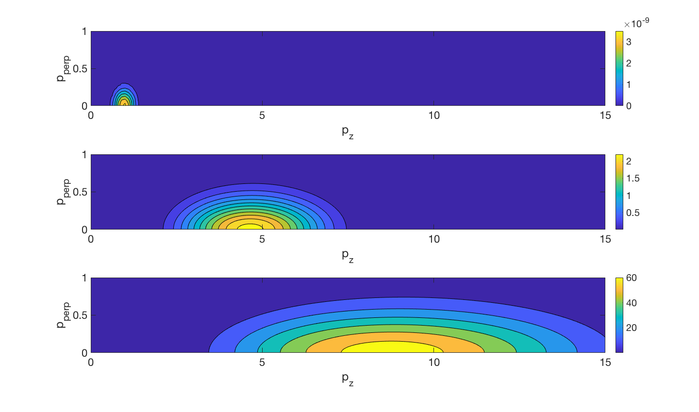
In Figure 2, the distribution function is displayed for different magnitudes of the electric field. As we can see, the contour curves are centered around an average value of that is higher for a stronger electric field. Moreover, the characteristic spread in and are both increasing with a stronger electric field. The effective mass added in the production process is proportional to the average value of , which in turn is proportional to the spread in Since this is dependent on the magnitude of the electric field, we can deduce that the error introduced by neglecting is dependent on the magnitude of the electric field. In Figure 3 we have quantified this observation by plotting , the spread in , as a function of . Loosely equating with the added effective mass of the pairs, gives a quick way to assess the accuracy in the common approximation of dropping the dependence on . In principle, the spread in momentum also depend on the length of the pulse duration. However, the dependence on the pulse duration is more or less negligible, and hence we omit plotting the result.
A consequence of omitting the perpendicular momentum appears when studying the number density of produced pairs. For the general expression, we have
| (60) |
and we must use the simplified expression
| (61) |
when there is no dependence on perpendicular momentum. However, the pair-production rate depends on the width of the distribution in perpendicular momentum space, which in turn depends on the magnitude of the electric field. As a result, the pair production rate with the perpendicular momentum omitted, and the full expression will scale differently with the electric field magnitude. In Fig. 4 we have studied this effect in the local density approximation using the same electric field profile as before. As can be seen, there is a general overestimation of the number of pairs using the approximation of parallel momentum only. To some extent the general overestimation could be fixed quite easily by introducing an overall correction factor in the evolution equation. However, for a self-consistent model with a dynamically varying electric field, we can not in general compensate for the fact that the overestimation of the produced pairs is dependent on the electric magnitude. As seen in Fig. 4, this overestimation is considerably larger for a weaker electric field.
Naturally, more figures of the perpendicular momentum dependence can be produced. Still, the ones we have chosen should be enough to give a reasonable picture of the significance of the perpendicular momentum in basic pair-production processes of the Schwinger-type.


V Summary and Discussion
In this paper, we have studied the DHW-formalism in the 1D electrostatic limit. It turns out that for this case, the 16 scalar equations of the general theory can be reduced to four scalar equations given in (II.3), which only needs to be complemented by Ampere’s law (27). Systems similar to Eqs. (II.3) have been studied previously, e.g. by Ref. Gies 2, who, however, did not include the dependence on perpendicular momentum. While a perpendicular momentum dependence was included in Ref. Gies, this paper only studied the homogeneous limit. Also, none of these works treated the field self-consistently by simultaneously solving (27).
To demonstrate the versatility of Eqs. (II.3)-(27), we first applied the system to linearized electrostatic waves in plasmas. The dispersion relation was derived, and shown to agree with well-known limiting cases. The issue of re-normalization, which is needed to treat the ultra-violet divergences associated with the vacuum background, is left for a future paper, however. In this context, it should be pointed out that a quantum-relativistic treatment of plasma waves is needed for very high plasma densities, such that the Fermi velocity is relativistic, as is the case for e.g. dense astrophysical objects.
For problems of pair-production in a given field, it has been common to neglect the perpendicular momentum dependence, see e.g. Refs. Gies 2. While this is a rather natural simplification, as the perpendicular momentum merely adds some extra mass to the pairs, nevertheless the accuracy of this approximation might not be very high. Studying Eqs. (II.3) for a given electric pulse with a temporal sech-profile, it is found that the approximation often is a useful one. Nevertheless, it is somewhat problematic to omit the perpendicular momentum dependence, as the error in the pair-production rate induced by this omission depends on the parameters of the problem. Specifically, for weakly inhomogeneous systems (such that the local density approximation is applicable), the perpendicular momentum of the generated pairs is close to linearly proportional to the electric field (cf. fig 3.) As a result, there is a general overestimation of the produced pairs when the perpendicular momentum is overlooked. While, in principle, a correction factor could be introduced to compensate for the overestimation, such a solution is not entirely satisfactory, as the correction factor would be dependent on the electric field magnitude, that could be varying dynamically in a self-consistent field model.
The broader conclusion from the present study, is that the equation system (II.3)- (27) provides a useful basis for studying pair-creation in a plasma medium self-consistently. However, for field-strengths sufficiently high to give appreciable pair-production, the plasma dynamics will become strongly nonlinear. Thus, in order to study pair-production in a plasma, the analytic treatment of the present paper must be replaced by a numerical approach.
References
- (1) P. Zhang, S. S. Bulanov, D. Seipt, A. V. Arefiev, and A. G. R. Thomas, Phys. Plasmas. 27, 050601 (2020).
- (2) I. S. Elkamash, F. Haas, and I. Kourakis, Phys. Plasmas. 24, 092119 (2017).
- (3) Y. Shi, J. Xiao, H. Qin, and N.J. Fisch, Phys. Rev. E. 97, 053206 (2018).
- (4) http://www.extreme-light-infrastructure.eu/.
- (5) Dunne, Gerald V. ”New strong-field QED effects at extreme light infrastructure.” The European Physical Journal D 55.2 (2009): 327.
- (6) http://xfel.eu.
- (7) Ringwald, Andreas. ”Pair production from vacuum at the focus of an X-ray free electron laser.” Physics Letters B 510.1-4 (2001): 107-116.
- (8) D. Del Sorbo, D. Seipt, T. G. Blackburn, A. G. R.Thomas, C. D. Murphy, J. G. Kirk, and C. P. Ridgers, Phys. Rev. A 96, 043407 (2017).
- (9) D. D. Sorbo, D. Seipt, A. G. R. Thomas,and C.P.Ridgers, Plasma Phys. Control. Fusion 60, 064003 (2018).
- (10) Y.-F. Li, R. Shaisultanov, K. Z. Hatsagort-syan, F. Wan, C. H. Keitel, and J.-X. Li, Phys. Rev. Lett. 122, 154801 (2019).
- (11) V Dinu, C Harvey, A Ilderton, M Marklund, G Torgrimsson, Phys. Rev. Lett. 116, 044801 (2016).
- (12) Hebenstreit, Florian, Reinhard Alkofer, and Holger Gies. ”Schwinger pair production in space-and time-dependent electric fields: Relating the Wigner formalism to quantum kinetic theory.” Physical Review D 82.10 (2010): 105026.
- (13) Sheng, Xin-li, et al. ”Wigner function and pair production in parallel electric and magnetic fields.” Physical Review D 99.5 (2019): 056004.
- (14) Sheng, Xin-li, et al. ”Wigner functions for fermions in strong magnetic fields.” The European Physical Journal A 54.2 (2018): 1-12.
- (15) Hebenstreit, Florian, Reinhard Alkofer, and Holger Gies. ”Particle self-bunching in the Schwinger effect in spacetime-dependent electric fields.” Physical review letters 107.18 (2011): 180403.
- (16) Hebenstreit, Florian. ”Schwinger effect in inhomogeneous electric fields.” arXiv preprint arXiv:1106.5965 (2011).
- (17) Kohlfürst, Christian. ”Effect of time-dependent inhomogeneous magnetic fields on the particle momentum spectrum in electron-positron pair production.” Physical Review D 101.9 (2020): 096003.
- (18) Aleksandrov, Ivan A., and Christian Kohlfürst. ”Pair production in temporally and spatially oscillating fields.” Physical Review D 101.9 (2020): 096009.
- (19) Bloch, J. C. R., et al. ”Pair creation: Back reactions and damping.” Physical Review D 60.11 (1999): 116011.
- (20) Asenjo, Felipe A., et al. ”Semi-relativistic effects in spin-1/2 quantum plasmas.” New Journal of Physics 14.7 (2012): 073042.
- (21) Manfredi, Giovanni, Paul-Antoine Hervieux, and Jérôme Hurst. ”Phase-space modeling of solid-state plasmas.” Reviews of Modern Plasma Physics 3.1 (2019): 13.
- (22) Ekman, Robin, F. A. Asenjo, and Jens Zamanian. ”Relativistic kinetic equation for spin-1/2 particles in the long-scale-length approximation.” Physical Review E 96.2 (2017): 023207.
- (23) Ekman, Robin, et al. ”Relativistic kinetic theory for spin-1/2 particles: Conservation laws, thermodynamics, and linear waves.” Physical Review E 100.2 (2019): 023201.
- (24) Bialynicki-Birula, Iwo, Pawel Gornicki, and Johann Rafelski. ”Phase-space structure of the Dirac vacuum.” Physical Review D 44.6 (1991): 1825.
- (25) Vasak, David, Miklos Gyulassy, and Hans-Thomas Elze. ”Quantum transport theory for Abelian plasmas.” Annals of Physics 173.2 (1987): 462-492.
- (26) Kluger, Yuval, Emil Mottola, and Judah M. Eisenberg. ”Quantum Vlasov equation and its Markov limit.” Physical Review D 58.12 (1998): 125015.
- (27) Smolyansky, S. A., et al. ”Dynamical derivation of a quantum kinetic equation for particle production in the Schwinger mechanism.” arXiv preprint hep-ph/9712377 (1997).
- (28) Sauter, Fritz. ”On the behavior of an electron in a homogeneous electric field in Dirac’s relativistic theory.” Zeit. f. Phys 69 (1931): 742.
- (29) Schwinger, Julian. ”On gauge invariance and vacuum polarization.” Physical Review 82.5 (1951): 664.
- (30) How slow the variations need to be for Section II.1 to apply is not obvious. This issue will be discussed in a forthcoming paper, where we will argue that for sufficiently intense fields, the temporal scale may even be allowed to approach and surpass the Compton scale.
- (31) Melrose, Donald B., and Jeanette I. Weise. ”Response of a relativistic quantum magnetized electron gas.” Journal of Physics A: Mathematical and Theoretical 42.34 (2009): 345502.
- (32) Schmidt, S., et al. ”A quantum kinetic equation for particle production in the Schwinger mechanism.” International Journal of Modern Physics E 7.06 (1998): 709-722.