Prospect-theoretic Q-learning Note: The work of VSB was partially supported by the S. S. Bhatnagar Fellowship from the Government of India.
Abstract
We consider a prospect theoretic version of the classical Q-learning algorithm for discounted reward Markov decision processes, wherein the controller perceives a distorted and noisy future reward, modeled by a nonlinearity that accentuates gains and under-represents losses relative to a reference point. We analyze the asymptotic behavior of the scheme by analyzing its limiting differential equation and using the theory of monotone dynamical systems to infer its asymptotic behavior. Specifically, we show convergence to equilibria, and establish some qualitative facts about the equilibria themselves.
Keywords:
Q-learning; prospect theory; cooperative o.d.e.; monotone dynamics; stable equilibria1 Introduction
Traditional reinforcement learning schemes are concerned with the actions of rational agents seeking to maximize their expected rewards. While these rational agents are risk neutral, reinforcement learning has also been studied under risk-sensitive (risk averse) policies [1, 2, 3]. But according to prospect theory [4] and its sibling cumulative prospect theory [5], human beings perceive risk differently in different scenarios: they can be risk seeking in some situations and risk averse in others. (See also [6, 7].) In this work, we study classical Q-learning for Markov decision processes [8], one of the early reinforcement learning algorithms, from a prospect theoretic viewpoint, i.e., when the future returns are distorted using an ‘S-shaped’ valuation map that increases perceived gains and decreases perceived losses.
Previous works [2, 3] applying such prospect theoretic valuation maps worked with certain restrictive assumptions. For example, [2] does not allow for steep valuation maps and high discount factors for future rewards. On the other hand, [3] changes the original Q-learning scheme in a manner that ensures convergence, but the formulation is a departure from the original paradigm as we point out later. In this work, we study the asymptotic behavior of Q-learning scheme when these additional restrictions and/or modifications are dropped. Naturally, we lose global convergence to a single equilibrium, but nevertheless we are able to characterize the asymptotic behavior in qualitative terms to a significant extent. The tools we use are the o.d.e. (for ‘Ordinary Differential Equations’) approach to stochastic approximation [9, 10] (See [11] for a textbook treatment) and monotone dynamical systems [12, 13, 14] to show convergence of the iteration to the set of equilibria and the structure of the latter set.
Our motivation for this study is twofold. The first is the classical motivation behind learning models in economics, viz., to build simple dynamic models to study the qualitative behaviour of boundedly rational macroeconomic agents [15]. Some of the interesting insights we obtain are that the learning in fact equilibrates (i.e., does not get into more complicated behavior such as cycling or worse, strange attractors), though not to a unique equilibrium. Furthermore, the choice of equilibrium depends on the initial condition which is characterizable at least in the cases when they are too high or too low in a certain sense. The equilibration of our model also has a flavor of rational expectations equilibrium [16], which may be an interesting analogy to pursue further.
Secondly, with algorithms taking over from humans in many spheres of human activity, there are ‘human in the loop’ scenarios such as e-commerce, crowdsourced decision making, recommendation networks, etc., where the empirically validated aspects of human judgement such as prospect theory must be factored in. This is so both when not doing so will lead to erroneous predictions and ipso facto erroneous decisions, and when the correct outcomes of human peculiarities can lead to undesired outcomes and you want to correct for them. For this, a good theoretical groundwork in terms of mathematical models of behavioral dynamics are important.
The need for this is already felt in the rapidly increasing literature that tries to factor in extending prospect theoretic aspects, e.g., in finance [17, 18], game theory [19, 20, 21, 22, 23], the newsvendor problem [24, 25, 26, 27], energy exchange mechanisms [28], etc., the works in prospect theoretic reinforcement learning are relatively few. In addition to those mentioned above, one interesting effort, albeit not in Markov decision theoretic framework, is [29]. See also [30, 31, 32] for other interesting takes on this theme. See [33] and [34] for textbook treatments of prospect theory and reinforcement learning resp., where further pointers to literature in the respective fields can be found.
In the next section, we give a short introduction to Q-learning and briefly, the aspects of prospect theory relevant here. In Section 3, we first present the modified Q-learning scheme and then study its limiting o.d.e. We then use results from monotone dynamical systems to show its convergence to equilibrium points. Then, in Section 4, we show results regarding stability, location and the number of equilibrium points for this scheme. In Section 5, we give a summary of the numerical simulations and comment on our observations. In Section 6, we discuss an alternative modification of the prospect theoretic Q-learning iteration where the total reward is prospect theoretically distorted, not only the future returns.
Notation: For ease of reference, we list the key notation used in the paper in the following table.
| Key Notation | |
|---|---|
| Controlled Markov chain | |
| Control process | |
| Finite state space with cardinality | |
| Finite action space with cardinality | |
| Discount factor | |
| Reward for choosing action at state | |
| min, resp. max of | |
| The constant | |
| Value function (see (1)) | |
| Q-values (see (2)) | |
| Dynamic programming operator for | |
| Stepsize sequence | |
| Number of times action is chosen at | |
| state till iteration | |
| S-shaped map (see Figure 1) | |
| i.i.d. noise concentrated in | |
| Parameter for epsilon-greedy policy (see (13)) | |
| Diagonal matrix for time scaling under | |
| asynchrony | |
2 Background
2.1 Q-Learning
We sketch the derivation of Watkins’ Q-learning algorithm [8] for discounted reward Markov decision processes, as a backdrop for our work. Consider a controlled Markov chain on a finite state space , governed by a control process in a finite action space , with controlled transition kernel with . The controlled Markov property is
Let be a discount factor and the per stage reward. For future reference, we denote by the minimum and maximum values of , which we assume are distinct (i.e., is not a constant). The infinite horizon discounted reward problem is to maximize
over all as above, called ‘admissible controls’. This maximum for is denoted by . The ‘value function’ then satisfies the dynamic programming equation
| (1) |
can be computed by, e.g., the value iteration algorithm
beginning with any guess . In reinforcement learning, one seeks a data-driven analog of this, where the nonlinearity due to the ‘max’ operator on the right causes problem because the conditional expectation is inside the nonlinearity.11 1 except in special circumstances that allow a ‘post-decision state’ formulation, see [35]. This obstructs any kind of empirical conditional averaging. One way around is to define the Q-values as the expression in square brackets on the right in (1), i.e.,
These satisfy their own dynamic programming equation
| (2) |
In turn, this can be solved by the ‘Q-value iteration’
where now the conditional expectation w.r.t. is outside the max. This facilitates a data driven learning (or stochastic approximation) version as follows. First, when the current state is and the control chosen is , one replaces the conditional expectation on the right hand side by an evaluation at the (real or simulated) next state , i.e.,
leaving or unchanged. The scheme is then stabilized by making it incremental, i.e., by replacing the full move suggested by the right hand side by a convex combination of it with the previous iterate , with a small weight on the former. This leads to the classical Q-learning algorithm
| (3) | |||||
Here is the ‘indicator function’ which is if ‘’ holds and otherwise. With the usual Robbins-Monro conditions on the stepsizes ,
| (4) |
this becomes a stochastic approximation algorithm. It is asynchronous because only the component corresponding to the current state-action pair is updated at each time. A variant is
| (5) | |||||
where is the ‘local clock’ at . Suppose that for some ,
| (6) |
This ensures ‘sufficient exploration’ in a precise sense, i.e., all state-action pairs are sampled ‘comparably often’. Under some additional restrictions on (see Chapter 7, [11]), (5) tracks the ordinary differential equation (ODE)
| (7) |
where suitably vectorized, is the dynamic programming operator for Q-values given by
| (8) |
for , also suitably vectorized. It can be seen that is a max-norm contraction:
and therefore has a unique fixed point that satisfies (2). This can be shown to be the globally asymptotically stable equilibrium of (7), from which the a.s. convergence of to can be inferred (see [11], pp. 129-130). A similar analysis also aplies to (3) except that the limiting ODE becomes
where:
- 1.
- 2.
which is an -contraction with contraction coefficient and a unique common fixed point .
This can be analyzed similarly to (7), but we avoid these complications and stick to (7), because they are not central to our main goals here.
2.2 Prospect Theory
Expected Utility Theory assumes that individuals behave rationally in order to maximize their expected utility. On the other hand, prospect theory [4, 36, 37, 33] aims to describe the actual, empirically validated behavior of people. Prospect theory replaces the utility function with a valuation map over gains and losses defined with respect to a reference point, which is the inflection point of the S-shaped curve in our case. The marginal impact of change in value diminishes with distance from the reference point. Similar to expected utility theory, concavity for gains contributes to risk aversion for gains. On the other hand, convexity for losses contributes to risk seeking behavior.22 2 In economics, concave utility function implies risk aversion because for stochastic returns denoted by , Jensen’s inequality leads to , meaning ‘sure returns’ fetch greater utility than random or risky returns . Analogous statement applies to convex and risk seeking behavior.

We incorporate these ideas into the Q-learning scheme above by passing the estimated future returns through an S-shaped continuous and continuously differentiable map (see Figure 1). What we take to be ‘estimated future returns’ is, however, a non-unique choice. Some possibities are:
- 1.
. Prima facie, this seems natural because this is precisely the term that depends on the next state, i.e., the ‘future’. This leads to the scheme
(9) - 2.
. This is the net estimate of future returns including the immediate reward. This leads to
(10) - 3.
. This is the estimate of the incremental future reward. This leads to
(11) This, however, goes against the spirit of the derivation of (5) in the preceding section because the update is no longer a convex combination of the previous iterate and a correction term. Nevertheless, it has been used in the literature [3]. We do not pursue this variant here.
Our interest is in the qualitative analysis of the asymptotic behavior of such algorithms as reflected in the limiting o.d.e. Any of the above leads to a monotone dynamics and our analysis applies, though the actual locations of the equilibria may shift. This is confirmed by our numerical experiments. We mostly focus on the first model.
In fact, we tweak even this model a little by adding noise. This is detailed in the next section.
3 Prospect theoretic Q-learning
3.1 Modified Q-learning scheme
Let be as above. We shall make the additional assumption that the graph of the Markov chain remains irreducible under all control choices at the nodes. Consider the prospect theoretic scheme:
| (12) | |||||
where is -valued zero mean i.i.d. noise. Each is distributed according to a continuously differentiable density concentrated on a finite interval for some . is chosen according to an epsilon-greedy policy, i.e., for a prescribed ,
| (13) |
where , with ties broken by choosing a maximizer with equal probability. We ignore the latter possibility henceforth for sake of simplicity.
The ‘noise’ can be justified as being caused by limited information, noisy measurements, etc. It serves a useful mathematical purpose here, as we note later.
Define and let be continuously differentiable.
Lemma 3.1.1.
If , then .
Proof.
Note that the Q-learning iteration can be written as:
| (14) |
So is a convex combination of
and . Now, if , then
Hence . The claim follows. ∎
We assume that the Q-learning iteration was initiated in the set . As shown in Chapter 2 of [11], since is Lipschitz continuous (it is continuously differentiable with bounded first derivative), and , the iteration (12) almost surely tracks the asymptotic behavior of the o.d.e. :
| (15) | |||||
where . The above implicitly defines the maps , in fact, . The integral is a convolution w.r.t. a continuously differentiable function, which makes it continuously differentiable.
Lemma 3.1.2.
When initiated in the set , o.d.e. (15) stays in the set .
Proof.
We can apply the following inequality on the derivative of :
Its discretization can be written as:
This implies that if , then . So, if initiated in the set , (and its limit, the o.d.e.) stays in the set . ∎
The Jacobian matrix of (resp., ) at is (resp., ), where is the identity matrix and for is the matrix whose th element is
| (16) | |||||
The continuous differentiability of was facilitated by the presence of the noise , which allows us to exploit the theory of monotone dynamical systems that is available when it holds. For that are only Lipschitz, such theory appears to be lacking.
3.2 Monotonicity and its consequences
We use the following notion of cooperative o.d.e. from [14]:
Definition 1.
(Cooperative o.d.e.) An o.d.e. of the form is a cooperative o.d.e. if
and the Jacobian matrix for is irreducible.
Lemma 3.2.1.
When the controlled Markov chain is irreducible, (the Jacobian of F) is a non-negative irreducible matrix and o.d.e. (15) is a cooperative o.d.e.
Proof.
Since , it follows that is a non-negative matrix. can be written as the product of the following two matrices: a non-negative matrix where and a positive diagonal matrix , where is times the integral in equation (16)). Since the Markov chain is irreducible, the matrix is irreducible and hence, the matrix will be irreducible. Since the off-diagonal terms of are non-negative and the Jacobian is irreducible, (15) is a cooperative o.d.e. ∎
Corollary 3.2.0.1.
The dynamical system described by (15) is monotone in the sense that if are two solutions with componentwise, then componentwise .
This follows from the results of [38]. The next theorem follows as a consequence of Theorem 2.1 from [12]
Theorem 3.2.1.
For initial conditions in an open dense set, the solutions of (15) converge to an equilibirium.
The same must then be true for the iterates of the discrete map which maps to . Since (15) is cooperative, this map is monotone. It is also ‘order compact’ in the sense of [13], section 5.1, because it maps an order interval, i.e., a set of the form componentwise to a bounded set. We define etc. analogously. Using part (b) of Theorem 5.6 from [13], the following holds:
Theorem 3.2.2.
Since the dynamics preserves order, it follows that for satisfying (15), and likewise, . If , since both are fixed points (i.e., equilibria) for the dynamics, by monotonicity. Since the map is continuous, the following theorem and its corollary hold:
Theorem 3.2.3.
(Order Interval Trichotomy, Theorem 5.1 from [13]) At least one of the following holds:
Corollary 3.2.3.1.
(Corollary 5.2 from [13]) If both and are stable, then there is at least one more equilibrium such that .
4 Equilibrium Points
4.1 Regions with stable equilibria
As our discrete map is the time- map of a differential equation with smooth right hand side, the stability of its equilibria, which are the same as equilibria of the differential equation, can be analyzed by looking at the linearization of at the equilibrium, i.e., the eigenvalues of the Jacobian matrix evaluated at the equilibrium. We have the following interesting observation from the foregoing.
Theorem 4.1.1.
If , resp. , is hyperbolic, then it is stable.
Proof.
If (say) is hyperbolic, it is isolated by the inverse function theorem and has well defined stable and unstable manifolds in an open neighborhood, corresponding to the eigenvalues of in the left, resp. right half of the complex plane. Furthermore, if the dimension of the unstable manifold is (i.e., there is at least one unstable eigenvalue), then for all initial conditions in an open neighborhood of , the trajectories that are not initiated exactly on the stable manifold eventually move away from . Since the dimension of the stable manifold is strictly less than , this is so for initial conditions in an open dense subset of . We may further exclude from its intersection with the closed nowhere dense set where the convergence claim of Theorem 3.2.1 can fail and denote the resultant open dense subset of as . Denote the intersection of with the open cone componentwise, as , which will be an open set. Then implies that eventually moves away from . By monotonicity, componentwise componentwise by monotonicity. Since is the maximal equilibrium, if , it must hold that , a contradiction to the previous claim. Hence must be stable. The claim for is proved similarly. ∎
The following theorem gives bounds on the eigenvalues of :
Theorem 4.1.2.
(Perron-Frobenius Theorem [39]) Let A be a square non-negative irreducible matrix. Then
- 1.
has a real positive eigenvalue which is greater than or equal to the absolute value of any other eigenvalue of .
- 2.
where and , where denotes the sum of the elements of row of .
Let the sum of the row of be . Let and . Since is a non-negative irreducible matrix, there exists a real positive eigenvalue (dominant eigenvalue) for such that any other eigenvalue of has its absolute value (and hence its real part) smaller than or equal to , by Theorem 4.1.2. We also know that . For any eigenvalue of , is an eigenvalue of the Jacobian . So, the real part of all eigenvalues of are less than .
Since is an S-shaped function, we know that is typically small for sufficiently low or high values of . Thus for sufficiently low or high values of and can exceed in the mid-range. If , then we can use the results from [2] which show that there will exist only one equilibrium point in the set and it will be stable. In fact this follows easily from the contraction mapping theorem. We consider here the case where exceeds in the middle region. Define points in as the largest and smallest points, respectively, in such that .
Theorem 4.1.3.
There is at most one equilibrium point for (15) in the set . If such an equilibrium point exists, it will be a stable equilibrium and the maximal equilibrium point. Similarly, there is at most one equilibrium point for (15) in the set and if such an equilibrium point exists, it will be a stable equilibrium and the minimal equilibrium point.
Proof.
Let be any point in the set . Then componentwise. Since in this region, and hence, . Hence real parts of all eigenvalues of the Jacobian are negative. So any equilibrium point lying in this region will be hyperbolic and stable. Now suppose that there are two equilibria in the aforementioned set. The two points can be ordered or unordered. First we consider the case where they are ordered and . By Corollary 3.2.3.1, there exists another equilibrium point , such that . Then will also be a stable equilibrium and hence there will be more stable equilibrium points between , and between . Repeated application of this argument implies that we will have a continuum of non-isolated equilibria. But real part of all eigenvalues of the Jacobian are negative in this region, implying that all equilibria are isolated. This gives us a contradiction. Hence there cannot be two ordered equilibria in the region.
Now consider the other case in which there are two unordered equilibria in the region . We know that there exists such that all equilibrium points satisfy (Theorem 3.2.2). Since no ordering exists between and , they can’t be equal to . So, where both and lie in this region. But we have shown earlier that there cannot exist ordered equilibria in the region. So, at most one equilibrium point can exist in this region and that will be the maximal equilibrium point. Analogous statement for the set is proved similarly. ∎
Based on Theorem 4.1.3, we subsequently refer to the sets and as the lower and upper stable regions, respectively.
4.2 Additional results on stability of equilibria
Let points in be the smallest and the largest points in such that . In most cases, and will be same as and respectively, but we have defined them separately to take care of cases where in the intervals and .
Theorem 4.2.1.
Any equilibrium point in the region is an unstable equilibrium point.
Proof.
Let be any point in the set . Then, componentwise. Since in this region, and hence, . Thus at least one eigenvalue of has a positive real part. Therefore any equilibrium point in this region will be unstable. ∎
Let the maximum value of be attained at .
Theorem 4.2.2.
If all equilibrium points are hyperbolic and is convex, respectively, concave in the regions and , respectively, then there can exist at most one stable equilibrium point in the region . Similarly in the region , there can exist at most one stable equilibrium. If these exist, then they will be the minimal and maximal equilibrium points, respectively.
Proof.
Suppose there exist two stable equilibrium points in the region . Again, there are two possibilities: they can be ordered or unordered. Let us first consider the case where they are ordered, say . Since we have taken to be concave in the region, for any point , . Hence componentwise. Let and be the dominant eigenvalues of and respectively. Then implies that (Theorem A.9 from [39]). Since and are stable equilibria, and are less than 1, and hence . So, will also be a stable equilibrium. As shown in the proof of Theorem 4.1.3, this gives us a continuum of non-isolated equilibria, which contradicts our assumption that all equilibria are hyperbolic.
If there exist two unordered equilibrium points in the region, then there will exist another equilibrium point which will be the maximal equilibrium and will be stable, as we have assumed that all equilibria are hyperbolic. Applying the first part of this proof to and gives us a contradiction. Hence there can be at most one stable equilibrium point in the region . The same is true for the set . ∎
This theorem can also be applied where the valuation map is a traditional utility function which is either convex or concave in the whole domain. In our case, however, there can exist many other stable equilibrium points with some components below and some above .
Let be a point such that . Then . In the convex combination form of the iteration (3.1), note that if , then
and hence . Similar to Lemma 3.1.1, we note that if the iteration (12) is initiated in the set , then it will stay in this set. In the following theorem, we use this to provide a sufficient condition for a stable equilibrium point of (15) to exist in the upper stable region. For simplicity, define .
Theorem 4.2.3.
Proof.
In the region , and hence and can intersect at most once in the region. Such an intersection point would exist if . If , then that point will be and their will be no other intersection. Let this intersection point be called .
As stated before, when , then the iteration (12) would stay in the set when initiated in it. Similarly, if initiated in the set , the iteration stays in that set. Hence there exists an equilibrium point of (15) in this set. As proved in Theorem 4.1.3, there can be at most one equilibrium point in the set . Hence, if the equilibrium point in the set will be the stable maximal equilibrium point and whenever iteration (12) is initiated in the region , it will converge to this equilibrium point. ∎
Similar to , define . We have the following theorem relating and the lower stable region similar to Theorem 4.2.3:
Theorem 4.2.4.
Theorem 4.2.5.
If , then there exists only one equilibrium point of (15) in the set and it will lie in the region .
Proof.
We know that (by the definition of ) and hence implies that . From the proof of Theorem 4.2.3, we know that the curve and intersect only once in the region . Let this point of intersection be . For all , and hence,
For all , and hence,
So lies strictly above in the region and hence will be the only intersection of these two curves in the region . Consider any . Then its minimum component is in . Let this minimum component be (i.e., ). Since and ,
So there can be no equilibrium point of (15) which does not belong to . By Theorem 4.2.3, we know that there exists one stable equilibrium in the region . This will be the only equilibrium point and will be both the maximal and minimal equilibrium point of (15). ∎
5 Numerical Experiments
We numerically simulated our modified Q-learning scheme and the corresponding o.d.e. to verify our results and gain additional insights. We used the shifted and scaled version of sigmoid logistic function:
By modifying value of and , we explored the behavior of the Q-learning scheme with varying maximum value, steepness and midpoint of the curve, respectively. Both very small and large state and action spaces were explored with values of both and ranging from to . To satisfy (4), we chose as:
where is the ceiling function and the scaling by was chosen for faster convergence. The rewards were generated randomly in a given range set by fixing and . The transition matrix was generated randomly. We tried different values of the discount factor ranging from to . We used the raised cosine distribution for noise as we required the noise distribution to be continuously differentiable in a finite support. Noise was in general kept much smaller than the rewards . Finally, we used for the -greedy scheme.


We varied different parameters and studied the Q-learning iteration, the o.d.e. and their equilibrium points. These are some of our observations:
- 1.
As long as the conditions mentioned in the Section 3 are met, the Q-learning iteration and the o.d.e. converged to an equilibrium point and to the same point when initiated at the same point. In Figure 2, we plot a representative convergence plot of error vs. iterations where error for iteration is defined as: .
- 2.
Choice of and have an impact on the rate of convergence, but do not observably affect the equilibrium points.
- 3.
As expected, when either is too small or the function rises very gradually (i.e., in the whole region), then there exists only one equilibrium point (see Figure 3(3(a))). Even when exceeds in the middle region, we frequently observe only one equilibrium point in when the maximum value of the first derivative of is not very high.

(a) 
(b) Figure 3: and for two different cases: (3(a)) shows the case where rises gradually and . Only one equilibrium is observed in this case. (3(b)) shows the case where . Equilibria are observed in both lower and upper stable regions in this case. () - 4.
- 5.
Theorems 4.2.3 and 4.2.4 only provide sufficient (and not necessary) conditions for existence of equilibria in the upper and lower stable regions. And hence, even when , we frequently observe an equilibrium point in the upper stable region (see Figure 4).

(a) 
(b) Figure 4: in two different cases: (4(a)) shows the case where . (4(b)) shows the case where . In both cases, an equilibrium exists in the upper stable region. ()
5.1 Third stable equilibrium point
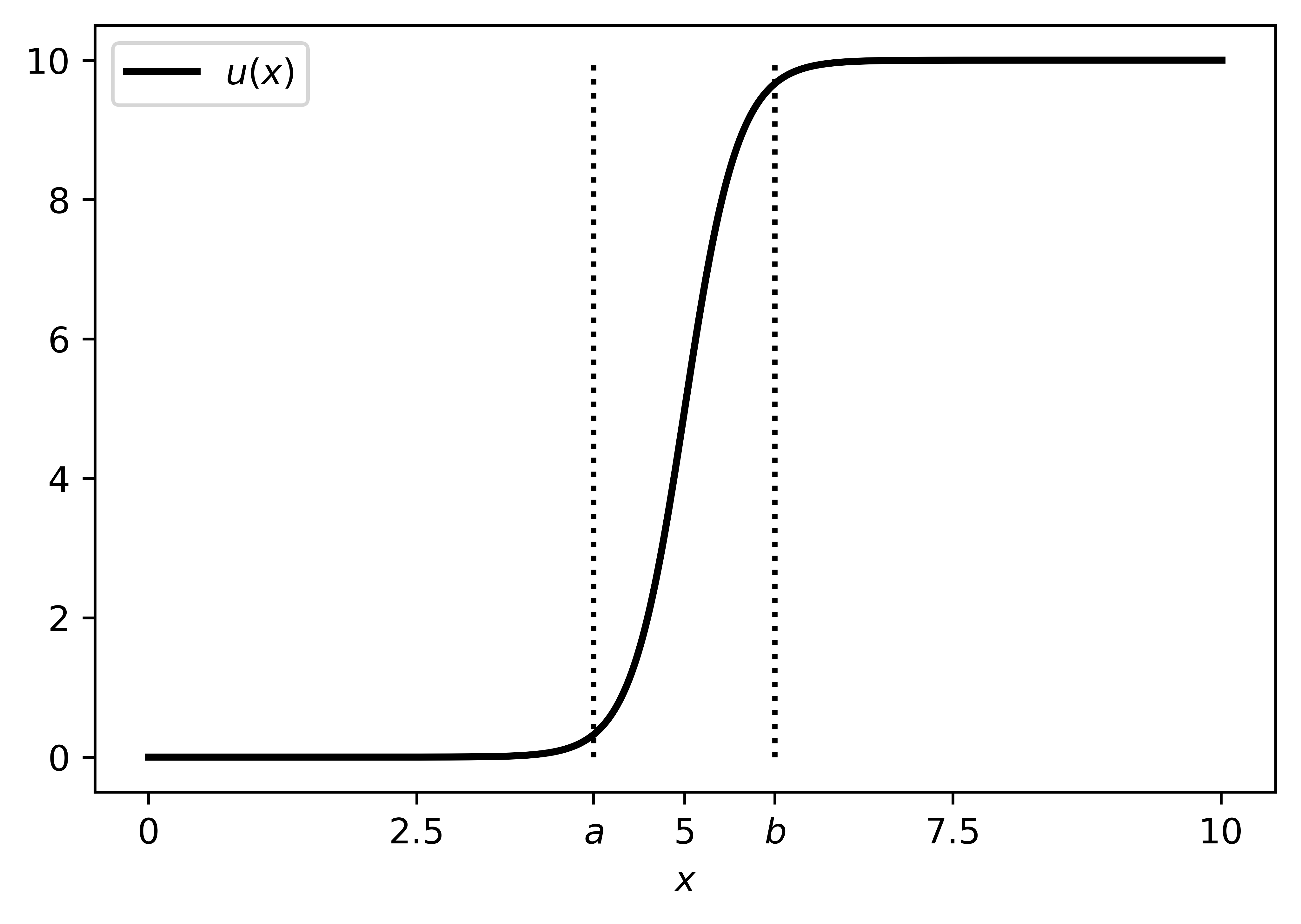
In general, we observed that convergence to any equilibrium point other than the maximal and minimal ones in the upper and lower stable regions is very rare. In our initial experiments, we noticed that the iteration converged either to the maximal or to the minimal equilibrium point. To confirm that the existence of a third stable equilibrium point is possible, we manually constructed and computed the equilibrium points for a small system . For further simplicity, we kept all rewards very close to (i.e., ) and fixed the value of to . We chose a very steep such that and . The function rises from to almost entirely between and (see Figure 5). This also ensured that the conditions in Theorems 4.2.3 and 4.2.4 are satisfied. The transition matrix was fixed so that for each state, the two actions are identical (i.e. where are the two actions for state ). For the transition probabilities we chose, we observed that there are four stable equilibria (two equilbria in addition to the maximal and minimal equilibria). When initiated in close vicinity to these additional equilibrium points, the iteration converges to them.
Apart from this above constructed case, we never observed the Q-learning iteration to converge to a stable equilibrium point other than the maximal or minimal. While three or more stable equilibria can exist for many systems, convergence to these points seems very infrequent in randomly generated test cases, suggesting a small domain of attraction. This is a purely empirical observation and it will be interesting to see if there is a fundamental reason for it being so.
We also compared our scheme with classical Q-learning for the same problem parameters (figures not included). The (necessarily unique) equilibrium of the latter was empirically found to be closer to the maximal equilibrium of the former than its minimal equilibrium, and either above or below it depending on the shape of the S-curve. For example, the equilibrium of classical Q-learning would be above the maximal equilibrium of our scheme if the S-curve had a very limited range. It became closer to the minimal equilibrium if we replaced reward maximization by cost minimization. Though the latter is merely a mathematical curiosity, it suggests that the preceding observations have more to do with ours being a maximization problem.
6 Alternative Formulation
In our original formulation, only the future returns are distorted using the prospect theoretic valuation map. We studied another formulation where the S-shaped curve is applied to the total returns, i.e., both the current rewards and the future returns are distorted.
6.1 Q-learning scheme and its convergence
The Q-learning iteration in this case is the following:
| (17) | |||||
In this case, and similar to Lemma 3.1.1, when initiated in the set , the Q-learning iteration stays in the set .
Iteration (17) tracks to the following o.d.e.:
| (18) | |||||
6.2 Stable regions
When , then the results from [2] again show that there will exist only one equilibrium point in the set . But when crosses in the middle regions, we observe behavior different from our original formulation. The upper and lower stable regions do not always exist in this case. As in Section 4.1, these stable regions are defined in the regions where the sum of each row of the Jacobian matrix is less than . This will be true when .
So, the upper stable region is defined as where and will exist if the following condition holds:
Condition 1.
Similarly the lower stable region is defined as where and will exist if:
Condition 2.
6.3 Numerical experiments
To simulate this formulation, i.e., iteration (17) and o.d.e. (18), we vary parameters as in Section 5. As expected, this scheme also converges to the equilibrium points. Most trends observed for the original scheme are observed here as well. For example, when rises very steeply and is large (greater than 0.7), we observe two equilibrium points, one each in the upper and lower stable regions.
An important difference between the two schemes lies in the values of the maximal and minimal equilibrium points. Since both the current and the future returns are distorted in this scheme, when the original scheme converged to large values of , this scheme converges to even larger values. Similarly, when the original scheme converged to small values, this scheme converges to even smaller values. This is observed in the simulations as well. When same parameters are set for both schemes, the maximal equilibrium point of the alternate formulation is higher than the maximal equilibrium for the original formulation.
7 Conclusions
In this work we studied classical Q-learning from a prospect theoretic viewpoint, i.e., when the valuation of future returns is distorted by an S-shaped subjective map. We then present conditions under which the iteration and its limiting o.d.e. converge to equilibrium points. Upper and lower stable regions are defined, in each of which at most one equilibrium exists and is stable. Additional results regarding the number and location of equilibria are also presented. We verify these results through simulations and make further comments regarding the observations. We finally study an alternative prospect theoretic scheme where both the current and future returns are distorted. A possible avenue for future work is to characterize conditions under which there are three or more equilibria and the scheme converges to an equilibrium point other than the maximal or minimal equilibrium. Also, it will be interesting to study the bifurcation phenomena that arise when the map is homotopically morphed from the identity map to an S-curve.
References
- [1] Mihatsch, O. and Neuneier, R., 2002. Risk-sensitive reinforcement learning. Machine Learning 49(2-3), 267-290.
- [2] Shen, Y., Stannat, W. and Obermayer, K., 2013. Risk-sensitive Markov control processes. SIAM Journal on Control and Optimization 51(5), 3652-3672.
- [3] Shen, Y., Tobia, M. J., Sommer, T. and Obermayer, K., 2014. Risk-sensitive reinforcement learning. Neural Computation 26(7), 1298-1328.
- [4] Kahneman, D. and Tversky, A., 2013. Prospect theory: An analysis of decision under risk. In Handbook of the Fundamentals of Financial Decision Making: Part I, 99-127.
- [5] Tversky, A. and Kahneman, D., 1992. Advances in prospect theory: Cumulative representation of uncertainty. Journal of Risk and Uncertainty 5(4), 297-323.
- [6] Dacey, R., 2003. The S-Shaped Utility Function. Synthese 135, 243–272.
- [7] Armstrong, J., and Brigo, D., 2019. Risk managing tail-risk seekers: VaR and expected shortfall vs S-shaped utility. Journal of Banking & Finance, 101, 122-135.
- [8] Watkins, C. J. C. H., 1989. Learning from delayed rewards. Ph.D. Thesis, King’s College, University of Cambridge, UK.
- [9] Derevitskii, D. P. and Fradkov, A. L., 1974 Two models for analyzing the dynamics of adaptation algorithms’. Automation and Remote Control 35, 59-67.
- [10] Ljung, L., 1977. Analysis of recursive stochastic algorithms. IEEE Transactions on Automatic Control 22, 551-575.
- [11] Borkar, V. S., 2008. Stochastic Approximation: A Dynamical Systems Viewpoint. Hindustan Publishing Agency, New Delhi, and Cambridge University Press, Cambridge, UK.
- [12] Hirsch, M. W. and Smith, H. L., 2003. Monotone systems, a mini-review, in Positive Systems (Benvenuti L., De Santis A. and L. Farina (eds)), Lecture notes on Control and Information sciences, Springer, Berlin-Heidelberg, 183-190.
- [13] Hirsch, M. W. and Smith, H., 2005. Monotone maps: a review. Journal of Difference Equations and Applications 11(4-5), 379-398.
- [14] Smith, H. L., 2008. Monotone Dynamical Systems: An Introduction to the Theory of Competitive and Cooperative Systems. American Mathematical Society, Providence, R. I.
- [15] Fudenberg, D. F. and Levine, D. K., 1998. The Theory of Learning in Games. MIT Press, Cambridge, MA.
- [16] Begg, D. K. H., 1982. The Rational Expectations Revolution in Macroeconomics: Theories Evidence. The Johns Hopkins University Press, Baltimore, MD.
- [17] He, X. D. and Zhou, X. Y., 2011. Portfolio choice under cumulative prospect theory: An analytical treatment. Management Science 57(2), 315-331.
- [18] Zhang, L., Zhang, H., and Hao, S., 2018. An equity fund recommendation system by combing transfer learning and the utility function of the prospect theory. The Journal of Finance and Data Science, 4(4), 223-233.
- [19] Phade, S. R. and Anantharam, V., 2018. Learning in Games with Cumulative Prospect Theoretic Preferences. arXiv preprint arXiv:1804.08005.
- [20] Phade, S. R. and Anantharam, V., 2019. On the geometry of Nash and correlated equilibria with cumulative prospect theoretic preferences. Decision Analysis 16(2), 142-156.
- [21] Phade, S. R. and Anantharam, V., 2020. Black-Box Strategies and Equilibrium for Games with Cumulative Prospect Theoretic Players. arXiv preprint arXiv:2004.09592.
- [22] Hota, A. R., Garg, S. and Sundaram, S., 2016. Fragility of the commons under prospect-theoretic risk attitudes. Games and Economic Behavior, 98, 135-164.
- [23] Tian, R., Sun, L. and Tomizuka, M., 2021. Bounded Risk-Sensitive Markov Games: Forward Policy Design and Inverse Reward Learning with Iterative Reasoning and Cumulative Prospect Theory. In AAAI Conference on Artificial Intelligence.
- [24] Vipin, B., and Amit, R. K., 2019. Describing decision bias in the newsvendor problem: A prospect theory model. Omega, 82, 132-141.
- [25] Nagarajan, M., and Shechter, S., 2014. Prospect Theory and the Newsvendor Problem. Management Science, 60(4), 1057-1062.
- [26] Shen, Y., Zhao, X., and Xie, J., 2017. Revisiting prospect theory and the newsvendor problem. Operations Research Letters, 45(6), 647-651.
- [27] Surti, C., Celani, A., and Gajpal, Y., 2020. The Newsvendor Problem: The Role of Prospect Theory and Feedback. European Journal of Operational Research, 287.
- [28] Xiao, L., Mandayam, N. B. and Poor, H. V., 2014. Prospect Theoretic Analysis of Energy Exchange Among Microgrids. IEEE Transactions on Smart Grid, 6(1), 63-72.
- [29] Prashanth, L. A., Jie, C., Fu, M., Marcus, S. and Szepesvári, C., 2016. Cumulative prospect theory meets reinforcement learning: Prediction and control. In Proc. International Conference on Machine Learning, 1406-1415.
- [30] Denrell, J. C., 2008. Reinforcement Learning Leads to Risk Averse Behavior. In Proceedings of the Annual Meeting of the Cognitive Science Society (Vol. 30, No. 30).
- [31] Feldmaier, J., Meyer, D., Shen, H., and Diepold, K., 2015. Reinforcement learning with preferences. In The 2nd Multidisciplinary Conference on Reinforcement Learning and Decision Making (pp. 143-147).
- [32] Ratliff, L. J., and Mazumdar, E., 2019. Inverse Risk-Sensitive Reinforcement Learning. IEEE Transactions on Automatic Control, 65(3), 1256-1263.
- [33] Wakker, P. P., 2010. Prospect Theory: For Risk and Ambiguity. Cambridge University Press, Cambridge, UK.
- [34] Bertsekas, d. P., 2019. Reinforcement Learning and Optimal Control. Athena Scientific, Belmont, MA.
- [35] Powell, W. B., 2007. Approximate Dynamic Programming: Solving the Curses of Dimensionality (2nd ed.). John Wiley and Sons, New York.
- [36] Fox, C. R. and Poldrack, R. A., 2009. Prospect theory and the brain. In Neuroeconomics, Academic Press, 145-173.
- [37] Ruggeri, K., Alí, S., Berge, M.L., Bertoldo, G., Bjørndal, L.D., Cortijos-Bernabeu, A., Davison, C., Demić, E., Esteban-Serna, C., Friedemann, M. and Gibson, S.P., 2020. Replicating patterns of prospect theory for decision under risk. Nature Human Behaviour, 1-12.
- [38] Hirsch, M. W., 1985. Systems of differential equations that are competitive or cooperative II: Convergence almost everywhere. SIAM Journal on Mathematical Analysis 16(3), 423-439.
- [39] Abramov, A. P., Balanced and Cyclical Growth in Models of Decentralized Economy, Springer International Publishing Switzerland 2014