跳到论文正文
W Papers独立论文阅读器 arXiv:2104.05095 论文正文 计算阅读时间 · 0%
引用这篇论文根据当前论文元数据生成,正式投稿前建议核对。


License: arXiv.org perpetual non-exclusive license
arXiv:2104.05095v2 [quant-ph] 29 Apr 2021

mnlargesymbols’164 mnlargesymbols’171

Operational approach to metastability

Katarzyna Macieszczak Affiliation: TCM Group, Cavendish Laboratory, University of Cambridge, J. J. Thomson Ave., Cambridge CB3 0HE, United Kingdom
Abstract

In this work, we introduce an information-theoretic approach for considering changes in dynamics of finitely dimensional open quantum systems governed by master equations. This experimentally motivated approach arises from considering how the averages of system observables change with time and quantifies how non-stationary the system is during a given time regime. By drawing an analogy with the exponential decay, we are able to further investigate regimes when such changes are negligible according to the logarithmic scale of time, and thus the system is approximately stationary. While this is always the case within the initial and final regimes of the dynamics, with the system respectively approximated by its initial and asymptotic states, we show that a distinct regime of approximate stationarity may arise. In turn, we establish a quantitative description of the phenomenon of metastability in open quantum systems. The initial relaxation occurring before the corresponding metastable regime and of the long-time dynamics taking place afterwards are also characterised. Furthermore, we explain how metastability relates to the separation in the real part of the master equation spectrum and connect our approach to the spectral theory of metastability, clarifying when the latter follows. All of our general results directly translate to Markovian dynamics of classical stochastic systems.

I Introduction

With continuing advances in the controllability of experimental systems such as ultracold atomic gases and Rydberg atoms as well as circuit quantum electrodynamics Pritchard et al. 2010; Barreiro et al. 2011; Blatt and Roos 2012; Britton et al. 2012; Dudin and Kuzmich 2012; Peyronel et al. 2012; Günter et al. 2013; Schmidt and Koch 2013, it is now possible to observe a broad range of nonequilibrium phenomena. In particular, open many-body quantum systems featuring both driving and dissipation give rise to stationary states no longer described by equilibrium distributions and phase diagrams featuring dissipative phase transitions Tomadin et al. 2011; Diehl et al. 2008; Torre et al. 2013. Furthermore, distinct timescales can arise in the relaxation towards stationary states, which are observed in experiments as plateaus in the dynamics of averages or time-correlations for system observables Sciolla et al. 2015. In equilibrium dynamics, this phenomenon of metastability can be understood as a consequence of multiple local minima present in the system free energy function, which leads to the existence of multiple metastable phases different from stable phases. For non-equilibrium dynamics, however, such a general description linking dynamic and static properties is elusive. Nevertheless, the dynamics is governed by a master equation with stationary states corresponding to its zero eigenvalues, and if there exists a large enough separation in the real part of its spectrum, metastable states can be similarly associated with its small eigenvalues Macieszczak et al. 2016; Rose et al. 2016; Minganti et al. 2018; Macieszczak et al. 2020 (for classical stochastic systems, see Refs. Gaveau and Schulman 1987; Gaveau and Schulman 1998; Bovier et al. 2002; Gaveau and Schulman 2006; Kurchan 2016).

In this work, we propose a general approach to metastability in finitely dimensional Markovian open quantum systems, which does not assume a separation in the spectrum of the corresponding master equation. Instead, motivated by experiments, we assume that changes in the system dynamics, quantified by changes in the averages of system observables, are negligible. This approach directly leads us to considering the distance in the space of states between system configurations at different times. Despite its abstractness, this perspective allows us to establish a simple but powerful analogy between open quantum dynamics and single-mode dynamics.

First, we argue how considering changes with respect to the logarithmic rather than linear scale of time, as already typically done, is in fact necessary due to Markovianity of the dynamics. Second, we show that an open quantum system is approximately stationary in the initial and final regimes of its dynamics, but there may exist a distinct time regime when the system changes negligibly and cannot be approximated by its initial or asymptotic states. This is achieved by obtaining bounds on the distance to initial and final regimes, which do not rely on perturbative arguments nor depend on the dimension of the system space. Therefore, we arrive at a general quantitative description of the phenomenon of metastability.

It is important to note that, albeit indirectly, the spectrum of the master equation can be accessed experimentally by measuring observable averages. Thus, our approach is also connected to the existence of a separation in the real part of the spectrum. In fact, we are able to derive general conditions on when the spectral theory as introduced in Refs. Macieszczak et al. 2016; Rose et al. 2016; Minganti et al. 2018; Macieszczak et al. 2020 is valid.

This paper is organized as follows. In Sec. II, we review Markovian dynamics of open quantum systems. In Sec. III, we consider single-mode dynamics and discuss regimes of its approximate stationary. In Sec. IV, we introduce the approach for quantifying changes in the dynamics of an open quantum system. We then define approximate stationarity and show how it may also correspond to metastability, in which case we characterise resulting metastable states, as well as, discuss the initial relaxation and the long-time dynamics. In Sec. V, we further connect metastability to the existence of a separation in the spectral decomposition of the system evolution. Finally, in Sec. VI, we clarify the relation between the operational approach and the spectral theory of metastability.

II Dynamics of open quantum systems

In this work, we consider time-homogeneous Markovian dynamics Lindblad 1976; Gorini et al. 1976 of finitely dimensional open quantum systems. Here, we briefly review a general structure of such dynamics and discuss the corresponding spectral decomposition.

II.1 Open quantum system

II.1.1 Master operator

An average state of the system at time tt, described by a density matrix ρt\rho_{t}, evolves according to a master equation

dd​t​ρt=ℒ⁡(ρt),\frac{d}{dt}\rho_{t}=\mathcal{L}(\rho_{t}), (1)

where the master operator Lindblad 1976; Gorini et al. 1976

ℒ⁡(ρ)≡−i⁡[H,ρ]+∑j[Jj​ρ​Jj†−12​{Jj†​Jj,ρ}].\mathcal{L}(\rho)\equiv-i[H,\rho]+\sum_{j}\left[{J}_{j}\rho{J}_{j}^{\dagger}-\frac{1}{2}\left\{{J}_{j}^{\dagger}{J}_{j},\rho\right\}\right]. (2)

Equation (2) arises for systems interacting weakly with an effectively memoryless environment (see, e.g., Ref. Gardiner and Zoller 2004), with HH denoting the system Hamiltonian and the jump operators Jj{J}_{j} providing coupling to the surrounding environment.

II.1.2 Dynamics

Since the master operator ℒ\mathcal{L} acts linearly on ρ\rho, the system state at time tt in Eq. (1) is given by

ρt=et​ℒ​(ρ0),\rho_{t}=e^{t\mathcal{L}}(\rho_{0}), (3)

where ρ0\rho_{0} denotes an initial state and we refer to et​ℒe^{t\mathcal{L}} an evolution operator. As at any time tt, ρt\rho_{t} is a density matrix, this requires the dynamics to preserve the Hermiticity [[ℒ⁡(ρ)]†=ℒ⁡(ρ†)[\mathcal{L}(\rho)]^{\dagger}=\mathcal{L}(\rho^{\dagger})], the trace [ℒ†​(𝟙)=0\mathcal{L}^{\dagger}(\mathds{1})=0] and the positivity of operators, which (together with complete positivity; cf., e.g., Ref. Wolf 2012) determines the structure of the master operator as that in Eq. (2).

In this work we assume that the system asymptotically reaches a time-independent state,

ρss=limt→∞ρt≡𝒫​ss​(ρ0),\rho_{\text{ss}}=\lim_{t\rightarrow\infty}\rho_{t}\equiv\mathcal{P}_{\text{\!ss}}(\rho_{0}), (4)

which we refer to as a stationary state. As a stationary state depends linearly on the initial conditions, we introduce the projection 𝒫​ss\mathcal{P}_{\text{\!ss}} on the set of stationary states. When ρss\rho_{\text{ss}} is unique, a generic situation in finite open many-body systems Spohn 1977; Evans 1977; Schirmer and Wang 2010; Nigro 2019, we simply have 𝒫​ss​(ρ)=ρss​Tr​(ρ)\mathcal{P}_{\text{\!ss}}(\rho)=\rho_{\text{ss}}{\mathrm{Tr}}(\rho). In general, however, stationary states correspond to decoherence free subspaces Zanardi 1997; Zanardi and Rasetti 1997; Lidar et al. 1998, noiseless subsystems Knill et al. 2000; Zanardi 2000 and disjoint stationary states (cf. Ref. Baumgartner and Narnhofer 2008).

If asymptotic states are time dependent, the general structure of their manifold remains the same, while their evolution is that of unitary dynamics within decoherence free subspaces and noiseless subsystems. This case will be discussed elsewhere.

III Single-mode dynamics

Before introducing the description of metastability in open quantum systems, we consider the dynamics of a single mode and discuss regimes of its approximate stationarity. Despite the simplicity of the considered dynamics, it is closely connected to the general evolution of an open quantum system as it shares its two crucial properties: the contractivity and its exponential form. Thus, the methods introduced here are directly applicable to the discussion of metastability that follows in Sec. IV. Furthermore, such a single-mode dynamics can be observed in an open quantum system by measuring system observables corresponding to eigenmodes of the master operator, which links the phenomenon of metastability to the spectral properties of the evolution, as we demonstrate in Sec. V.

While the regimes of approximate stationarity of a single mode correspond to times ’before’ and ’after’ the dynamics and thus can be considered trivial, they highlight a key aspect of the characterising the system evolution with respect to the logarithmic rather than linear scale of time, which directly translates to the formal definition of metastability in Sec. IV. Actually, as we show in Sec. V, metastability in an open quantum system may only occur at the overlap of either of these regimes for all of eigenmodes present in the dynamics.

Figure 1: Single mode and its approximate stationarity. A real single-mode dynamics is described by et​λe^{t\lambda} (red dashed) which decays with time tt for λ<0\lambda<0, so that the value of the function itself equals the distance to its asymptotic limit. As a consequence, the distance to its initial value of 11 (green dotted) increases with time. In the initial and final regimes et​λe^{t\lambda} is approximated by 11 and 00 respectively [areas shaded green and red, respectively, for c=0.1c=0.1 in Eq. (6)]. (a) The changes in the function (black solid) with respect to the linear scale of time, i.e., et​λ−e(t+δ​t)​λe^{t\lambda}-e^{(t+\delta t)\lambda} with a fixed δ​t≥0\delta t\geq 0, decay exponentially at the rate λ\lambda from the initial value 1−eδ​t​λ1-e^{\delta t\lambda}, so that they are negligible only in the final regime. (b) In contrast, the changes with respect to the logarithmic scale of time, e.g., et​λ−e2​t​λe^{t\lambda}-e^{2t\lambda} (black solid), are negligible both in the initial and final regimes. Furthermore, they equal the product of the distances to the initial and asymptotic values (green dotted and red dashed) and are bounded by 1/41/4. It follows that for cΔ=et​λ−e2​t​λc_{\Delta}=e^{t\lambda}-e^{2t\lambda} we have E+​(cΔ)=max⁡(et​λ,1−et​λ)E_{+}(c_{\Delta})=\max(e^{t\lambda},1-e^{t\lambda}) and E−​(cΔ)=min⁡(et​λ,1−et​λ)E_{-}(c_{\Delta})=\min(e^{t\lambda},1-e^{t\lambda}), and thus the bounds in Eq. (10) saturate [excluded values shaded grey; cf. Fig. 2(a)].

III.1 Dynamics

We now introduce the dynamics of a real single mode and identify initial and final regimes of its approximate stationarity. The dynamics is one dimensional and describes an exponential decay (see Figs. 1). We discuss the case of a complex mode, which corresponds to a spiral motion in a plane, in Appendix A.

We consider the dynamics given by et​λe^{t\lambda}, where we assume a negative rate λ<0\lambda<0. The exponential behaviour is analogous to the open quantum system dynamics in Eq. (3), while the rate condition ensures a constant asymptotic limit as in Eq. (4); cf. Fig. 1(a).

As the only timescale is given by −1/λ-1/\lambda, there are two regimes of approximate stationarity in the dynamics of a single mode (see Fig. 1). The initial regime takes place when the dynamics can be neglected and the function is approximated by its initial value 11. The final regime occurs for large enough times, so that the function has decayed close to its asymptotic limit of 00. We formally define the regimes by requiring that the difference of function values to its initial and asymptotic limit is not larger than

c≪1,c\ll 1, (5)

that is,

et​λ≥1−coret​λ≤c.e^{t\lambda}\geq 1-c\quad\text{or}\quad e^{t\lambda}\leq c. (6)

Therefore, the approximate stationarity occurs for

t⁡(−λ)≤−ln⁡(1−c)=c+…ort⁡(−λ)≥−ln⁡(c).t(-\lambda)\leq-\ln(1-c)=c+...\quad\text{or}\quad t(-\lambda)\geq-\ln(c). (7)

Here, the inequalities are valid for any 0<c<10<c<1 and correspond to distinct regimes for c<1/2c<1/2; we expanded up to linear in cc using Eq. (5).

III.2 Changes in time

The initial regime is finite, while the final regime is unbounded; cf. Fig. 1. Furthermore, in the initial regime corrections to their initial value grow linearly with time and proportionally to λ\lambda, while in the final regime the mode decays to its limit exponentially with time at this rate. Nevertheless, we now introduce a way to quantify how non-stationary is the dynamics, which allows to identify the initial and final regimes despite their differences.

To this aim we consider how the function changes with time, that is, |et1​λ−et2​λ||e^{t_{1}\lambda}-e^{t_{2}\lambda}| for t1≠t2t_{1}\neq t_{2}, and view it as approximately stationary when changes during a given time regime are negligible. In particular, we show that negligible changes with respect to the logarithmic scale of time for a real mode occur only in the initial and the final regimes of its dynamics [cf. Fig. 1(b)].

III.2.1 Linear scale

A crucial property of the dynamics of a single mode is its contractivity, that is, the decay of the distance between function values at different times when shifted forward in time, |e(t1+δ​t)​λ−e(t2+δ​t)​λ|≤|et1​λ−et2​λ||e^{(t_{1}+\delta t)\lambda}-e^{(t_{2}+\delta t)\lambda}|\leq|e^{t_{1}\lambda}-e^{t_{2}\lambda}| for δ​t≥0\delta t\geq 0; cf. Fig. 1(a). Thus, requiring that the function changes no more than a given distance, does not uniquely determine a time regime. In fact, a negligibly small change can be achieved after an arbitrary time, simply by considering time difference within the initial regime as |et1​λ−et2​λ|≤|e|t1−t2|​λ−1||e^{t_{1}\lambda}-e^{t_{2}\lambda}|\leq|e^{|t_{1}-t_{2}|\lambda}-1|, and such approximate stationarity can be seen as inherited from the initial regime. This issue remains when normalising |et1​λ−et2​λ||e^{t_{1}\lambda}-e^{t_{2}\lambda}| by the bigger (or the smaller) of the function absolute values, as this yields |e|t1−t2|​λ−1||e^{|t_{1}-t_{2}|\lambda}-1| (or |e−|t1−t2|​λ−1||e^{-|t_{1}-t_{2}|\lambda}-1|) dependent solely on the time difference.

III.2.2 Logarithmic scale

We now show that when the mode changes negligibly during a time interval at least of the order of the earlier time, it belongs either to the initial regime or the final regime; cf. Fig. 1(b). This is possible, as we are able to consider how the dynamics changes with respect to the logarithmic rather than the linear scale.

Indeed, for a real mode and

cΔ≪1,c_{\Delta}\ll 1, (8)

we consider time tt such that

et​λ−e2​t​λ≤cΔ.e^{t\lambda}-e^{2t\lambda}\leq c_{\Delta}. (9)

With E±​(cΔ)E_{\pm}(c_{\Delta}) denoting two solutions for the quadratic equation e2​t​λ−et​λ+cΔ=0e^{2t\lambda}-e^{t\lambda}+c_{\Delta}=0 with respect to et​λe^{t\lambda}, Eq. (9) then holds if and only if [see Fig. 1(b)]

et​λ≥E+​(cΔ)≡1+1−4​cΔ2=1−cΔ+…or\displaystyle e^{t\lambda}\geq E_{+}(c_{\Delta})\equiv\frac{1+\sqrt{1-4c_{\Delta}}}{2}=1-c_{\Delta}+...\quad\text{or}\quad (10a)
et​λ≤E−​(cΔ)≡1−1−4​cΔ2=cΔ+…,\displaystyle e^{t\lambda}\leq E_{-}(c_{\Delta})\equiv\frac{1-\sqrt{1-4c_{\Delta}}}{2}=c_{\Delta}+..., (10b)

where in the inequalities we assumed cΔ≤1/4c_{\Delta}\leq 1/4; we expanded up to linear order in cΔc_{\Delta} using Eq. (8).

Note that 1−E+​(cΔ)=E−​(cΔ)1-E_{+}(c_{\Delta})=E_{-}(c_{\Delta}), so that Eq. (9) holds if and only if tt belongs to the initial and final regimes in Eq. (6) with c=E−​(cΔ)c=E_{-}(c_{\Delta}). Furthermore, as et​λ−e2​t​λe^{t\lambda}-e^{2t\lambda} is the maximal change for times between tt and 2​t2t, we have that all times between tt and 2​t2t belong either to the initial regime with c=1−[E+​(cΔ)−cΔ]=E−​(cΔ)+cΔc=1-[E_{+}(c_{\Delta})-c_{\Delta}]=E_{-}(c_{\Delta})+c_{\Delta} or to the final regime with c=E−​(cΔ)c=E_{-}(c_{\Delta}). These regimes are distinct for cΔ<−2+5=0.236​…c_{\Delta}<-2+\sqrt{5}=0.236....

IV Operational approach to metastability

Metastability is typically considered to occur when there exists a pronounced time regime during which system states appear stationary. In this work, we introduce an operational approach to metastability in open quantum systems, which among others, allows us to formalize this definition.

We consider accessing a state of an open quantum system by measuring observables averages. This leads to a quantitative description of changes in the system dynamics in terms of the trace norm. In turn, this allows us to introduce initial and final regimes of the dynamics in analogy to the dynamics of a single mode discussed earlier. In contrast to that case, however, we find that a distinct regime of approximate stationarity may arise in the dynamics of an open quantum system, which we recognise as the phenomenon of metastability.

Using the operational approach, we are able to identify the set of metastable states and characterise both the timescales and the structure of dynamics before and after the metastable regime.

IV.1 Changes in time

We begin by discussing how an open quantum system changes during its evolution. We consider accessing a state of the system by measuring observable averages, since a state of a quantum system of with the space dimension DD can be reconstructed by measuring D2D^{2} linearly independent observables.

For an observable OO, the maximal change in the average of an observable OO within a given time regime t′≤t≤t′′t^{\prime}\leq t\leq t^{\prime\prime} is given by

𝒞Δ​(ρ0,O,t′′,t′)\displaystyle\mathcal{C}_{\Delta}(\rho_{0};O;t^{\prime\prime},t^{\prime}) ≡\displaystyle\equiv supt′′≤t1,t2≤t′|Tr⁡(O​ρt1)−Tr⁡(O​ρt2)|∥O∥max,\displaystyle\!\sup_{t^{\prime\prime}\leq t_{1},t_{2}\leq t^{\prime}}\!\!\frac{|{\mathrm{Tr}}(O\rho_{t_{1}})-{\mathrm{Tr}}(O\rho_{t_{2}})|}{\lVert O\rVert_{\max}},\qquad (11)

where ρ0\rho_{0} is initial system state. Here, we normalise by the max norm of the observable, ∥O∥max≡supρ0Tr⁡(O​ρ0)\lVert O\rVert_{\max}\equiv\sup_{\rho_{0}}{\mathrm{Tr}}(O\rho_{0}) (see Appendix B.1 and 11 1 Normalising changes of the observable average by supt≥0|Tr⁡(O​ρt)|\sup_{t\geq 0}|{\mathrm{Tr}}(O\rho_{t})| leads to larger values than in Eq. (11) and thus more restrictive definitions of the initial and final regimes as well as that of the metastability.).

Assuming that measuring of all observables is possible (or, equivalently, D2D^{2} linearly independent observables can be measured), the maximal change corresponds to the maximal distance between system states measured in the trace norm

𝒞Δ​(ρ0,t′′,t′)\displaystyle\mathcal{C}_{\Delta}(\rho_{0};t^{\prime\prime},t^{\prime}) ≡\displaystyle\equiv supO𝒞Δ​(ρ0,O,t′′,t′)\displaystyle\,\,\sup_{O}\,\,\mathcal{C}_{\Delta}(\rho_{0};O;t^{\prime\prime},t^{\prime}) (12)
=\displaystyle= supt′′≤t1,t2≤t′∥ρt1−ρt2∥.\displaystyle\sup_{t^{\prime\prime}\leq t_{1},t_{2}\leq t^{\prime}}\lVert\rho_{t_{1}}-\rho_{t_{2}}\rVert.

Indeed, |Tr⁡(O​ρt1)−Tr⁡(O​ρt2)|≤∥O∥max​∥ρt1−ρt2∥|{\mathrm{Tr}}(O\rho_{t_{1}})-{\mathrm{Tr}}(O\rho_{t_{2}})|\leq\lVert O\rVert_{\max}\lVert\rho_{t_{1}}-\rho_{t_{2}}\rVert, with the inequality saturated for O=Π+−Π−O=\Pi_{+}-\Pi_{-}, where Π+\Pi_{+} and Π−\Pi_{-} are the projections on the direct sum of eigenspaces of ρt1−ρt2\rho_{t_{1}}-\rho_{t_{2}} corresponding to positive and negative eigenvalues, respectively (see Appendix B.1). We note that there is no additional normalisation needed in Eq. (12), as for the system states ∥ρt∥=1\lVert\rho_{t}\rVert=1.

Assuming further the system can be initialised in any state (or, equivalently, D2D^{2} linearly independent initial states can be prepared), the maximal change in the dynamics 𝒞Δ​(t′′,t′)≡supρ0supO𝒞Δ​(ρ0,O,t′′,t′)\mathcal{C}_{\Delta}(t^{\prime\prime},t^{\prime})\equiv\sup_{\rho_{0}}\sup_{O}\mathcal{C}_{\Delta}(\rho_{0};O;t^{\prime\prime},t^{\prime}) captures by the distance between the corresponding evolution operators in the norm induced by the trace norm (see Appendix B.2),

𝒞Δ​(t′′,t′)\displaystyle\mathcal{C}_{\Delta}(t^{\prime\prime},t^{\prime}) =\displaystyle= supρ0supO𝒞Δ​(ρ0,O,t′′,t′)\displaystyle\,\,\sup_{\rho_{0}}\,\,\sup_{O}\,\,\mathcal{C}_{\Delta}(\rho_{0};O;t^{\prime\prime},t^{\prime}) (13)
=\displaystyle= supt′′≤t1,t2≤t′∥et1​ℒ−et2​ℒ∥.\displaystyle\sup_{t^{\prime\prime}\leq t_{1},t_{2}\leq t^{\prime}}\lVert e^{t_{1}\mathcal{L}}-e^{t_{2}\mathcal{L}}\rVert.

Here, the supremum is achieved for a pure initial state, ρ0=ρ02\rho_{0}=\rho_{0}^{2}.

We have that [cf. Eq. (11)]

𝒞Δ​(ρ0,O,t′′,t′)\displaystyle\mathcal{C}_{\Delta}(\rho_{0};O;t^{\prime\prime},t^{\prime}) =\displaystyle= supt′′≤t≤t′Tr⁡(O​ρt)∥O∥max−inft′′≤t≤t′Tr⁡(O​ρt)∥O∥max.\displaystyle\sup_{t^{\prime\prime}\leq t\leq t^{\prime}}\frac{{\mathrm{Tr}}(O\rho_{t})}{\lVert O\rVert_{\max}}\!-\!\!\!\inf_{t^{\prime\prime}\leq t\leq t^{\prime}}\frac{{\mathrm{Tr}}(O\rho_{t})}{\lVert O\rVert_{\max}}.\qquad (14)

Furthermore, as ∥et​ℒ∥=1\lVert e^{t\mathcal{L}}\rVert=1, the dynamics is contractive with respect to the trace norm, ∥ρt1+t−ρt2+t∥≤∥et​ℒ∥​∥ρt1−ρt2∥=∥ρt1−ρt2∥\lVert\rho_{t_{1}+t}-\rho_{t_{2}+t}\rVert\leq\lVert e^{t\mathcal{L}}\rVert\lVert\rho_{t_{1}}-\rho_{t_{2}}\rVert=\lVert\rho_{t_{1}}-\rho_{t_{2}}\rVert (see, e.g., Refs. Watrous 2005; Wolf 2012 or Appendix B.3). It then follows that [cf. Eqs. (12) and (13)]

𝒞Δ​(ρ0,t′′,t′)\displaystyle\mathcal{C}_{\Delta}(\rho_{0};t^{\prime\prime},t^{\prime}) =\displaystyle= supt′′≤t≤t′∥ρt′′−ρt∥,\displaystyle\sup_{t^{\prime\prime}\leq t\leq t^{\prime}}\lVert\rho_{t^{\prime\prime}}-\rho_{t}\rVert, (15)
𝒞Δ​(t′′,t′)\displaystyle\mathcal{C}_{\Delta}(t^{\prime\prime},t^{\prime}) =\displaystyle= supt′′≤t≤t′∥et′′​ℒ−et​ℒ∥.\displaystyle\sup_{t^{\prime\prime}\leq t\leq t^{\prime}}\lVert e^{t^{\prime\prime}\mathcal{L}}-e^{t\mathcal{L}}\rVert. (16)

The quantities in Eqs. (14), (15), and (16) grow when the time regime is enlarged, that is, when t′t^{\prime} increases or t′′t^{\prime\prime} decreases (see Fig. 2). In particular, for Eqs. (15) and (16), extending the length of the considered regime leads to at most a linear increase,

𝒞Δ​[ρ0;t′′,t′′+n⁡(t′−t′′)]\displaystyle\mathcal{C}_{\Delta}[\rho_{0};t^{\prime\prime},t^{\prime\prime}+n(t^{\prime}-t^{\prime\prime})] ≤\displaystyle\leq n​𝒞Δ​(ρ0,t′′,t′),\displaystyle n\,\mathcal{C}_{\Delta}(\rho_{0};t^{\prime\prime},t^{\prime}), (17)
𝒞Δ​[t′′,t′′+n⁡(t′−t′′)]\displaystyle\mathcal{C}_{\Delta}[t^{\prime\prime},t^{\prime\prime}+n(t^{\prime}-t^{\prime\prime})] ≤\displaystyle\leq n​𝒞Δ​(t′′,t′).\displaystyle n\,\mathcal{C}_{\Delta}(t^{\prime\prime},t^{\prime}). (18)

This follows from the contractivity of the dynamics; for t1,t2≥t′′t_{1},t_{2}\geq t^{\prime\prime} such that (n−1)​(t′′−t′)≤t1−t2≤n⁡(t′′−t′)(n\!-\!1)(t^{\prime\prime}-t^{\prime})\leq t_{1}-t_{2}\leq n(t^{\prime\prime}-t^{\prime}) we have ∥ρ⁡(t1)−ρ⁡(t2)∥≤∑l=1n−1∥ρ⁡[t2+l⁡(t′−t′′)]−ρ⁡[t2+(l−1)​(t′−t′′)]∥+∥ρ⁡(t1)−ρ⁡[t2+(n−1)​(t′−t′′)]∥≤n​𝒞Δ​(ρ0,t′′,t′)\lVert\rho(t_{1})-\rho(t_{2})\rVert\leq\sum_{l=1}^{n-1}\lVert\rho[t_{2}+l(t^{\prime}-t^{\prime\prime})]-\rho[t_{2}+(l-1)(t^{\prime}-t^{\prime\prime})]\rVert+\lVert\rho(t_{1})-\rho[t_{2}+(n-1)(t^{\prime}-t^{\prime\prime})]\rVert\leq n\mathcal{C}_{\Delta}(\rho_{0};t^{\prime\prime},t^{\prime}).

Finally, we note that for any time regime changes in the system state are bounded by

𝒞Δ​(ρ0,t′′,t′)\displaystyle\mathcal{C}_{\Delta}(\rho_{0};t^{\prime\prime},t^{\prime}) ≤\displaystyle\leq 2,\displaystyle 2, (19)

where the bound corresponds to the distance between any two orthogonal states. From Eq. (19) we obtain (cf. Fig. 2)

𝒞Δ​(t′′,t′)\displaystyle\mathcal{C}_{\Delta}(t^{\prime\prime},t^{\prime}) ≤\displaystyle\leq 2.\displaystyle 2. (20)

IV.2 Initial and final regimes

For any open quantum system, there always exist two time regimes where changes can be neglected. These are initial and final regimes, which can be defined in a direct analogy to the dynamics of a single mode.

IV.2.1 Definition

For a chosen observable OO and an initial state ρ0\rho_{0}, we consider the initial and final regimes by requiring that the normalised difference of the observable average Tr⁡(O​ρt){\mathrm{Tr}}(O\rho_{t}) to its initial value Tr⁡(O​ρ0){\mathrm{Tr}}(O\rho_{0}) or its asymptotic limit Tr⁡(O​ρss){\mathrm{Tr}}(O\rho_{\text{ss}}), respectively, is not larger than [cf. Eq. (5)]

𝒞≪1.\mathcal{C}\ll 1. (21)

The overlap of initial or final regimes for all observables and initial system states [cf. Eqs. (11), (12), and (13)] leads to the following.

The initial regime of the dynamics holds for t≤t0​(𝒞)t\leq t_{0}(\mathcal{C}), where t0​(𝒞)t_{0}(\mathcal{C}) is the shortest time such that ∥et0​(𝒞)​ℒ−ℐ∥=𝒞\lVert e^{t_{0}(\mathcal{C})\mathcal{L}}-\mathcal{I}\rVert=\mathcal{C} with ℐ⁡(ρ)≡ρ\mathcal{I}(\rho)\equiv\rho, and thus

∥et​ℒ−ℐ∥≤𝒞.\lVert e^{t\mathcal{L}}-\mathcal{I}\rVert\leq\mathcal{C}. (22)

The final regime of the dynamics holds for times

∥et​ℒ−𝒫​ss∥≤𝒞\lVert e^{t\mathcal{L}}-\mathcal{P}_{\text{\!ss}}\rVert\leq\mathcal{C} (23)

[due to the contractivity of the dynamics ∥et​ℒ−𝒫​ss∥\lVert e^{t\mathcal{L}}-\mathcal{P}_{\text{\!ss}}\rVert decays with time tt, so that Eq. (23) holds for all t≥tss​(𝒞)t\geq t_{\text{ss}}(\mathcal{C}) where tss​(𝒞)t_{\text{ss}}(\mathcal{C}) is the shortest time such that ∥etss​(𝒞)​ℒ−𝒫​ss∥=𝒞\lVert e^{t_{\text{ss}}(\mathcal{C})\mathcal{L}}-\mathcal{P}_{\text{\!ss}}\rVert=\mathcal{C}]. Note that the initial and final regimes are distinct for 𝒞<1/2\mathcal{C}<1/2 [note that ∥ℐ−𝒫​ss∥≤∥et​ℒ−ℐ∥+∥et​ℒ−𝒫​ss∥\lVert\mathcal{I}-\mathcal{P}_{\text{\!ss}}\rVert\leq\lVert e^{t\mathcal{L}}-\mathcal{I}\rVert+\lVert e^{t\mathcal{L}}-\mathcal{P}_{\text{\!ss}}\rVert and cf. Eq. (24) below; see Fig. 2(a)].
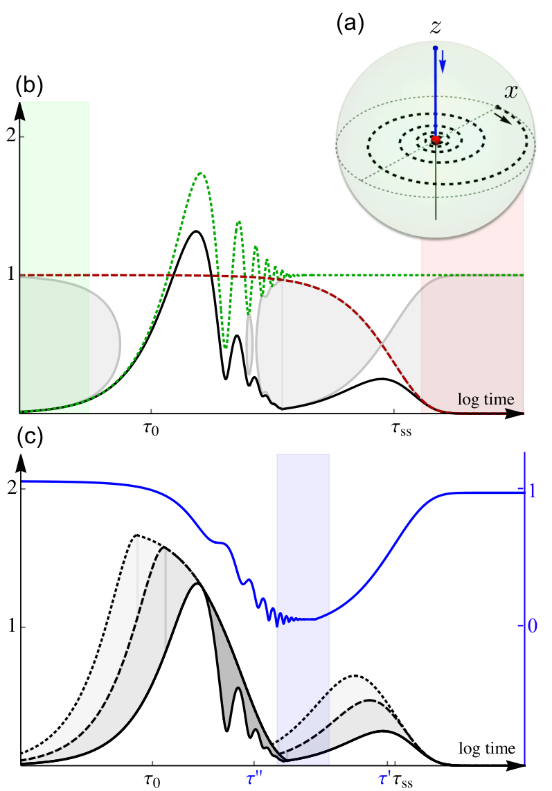
Refer to caption
Figure 2: Minimal open quantum system with metastability. We consider a spin-1/21/2 in the presence of magnetic field, H=−ω​SzH\!=\!-\omega S_{z}, whose uncorrelated-in-time fluctuations amount to dephasing, Jz=γ​SzJ_{z}\!=\!\sqrt{\gamma}S_{z}, and in contact with an infinite-temperature bath, J+=κ/2​S+J_{+}\!=\!\sqrt{\kappa/2}\,S_{+} and J−=κ/2​S−J_{-}\!=\!\sqrt{\kappa/2}\,S_{-}, where S±=Sx±SyS_{\pm}\!=\!S_{x}\pm S_{y} and SxS_{x}, SyS_{y}, SzS_{z} are the spin operators along xx, yy, zz axes, respectively. (a) The magnetisation along zz axis (blue solid) decays exponentially to 00 in correspondence with a real mode (λ=κ\lambda\!=\!\kappa; cf. Fig. 1), while along xx and yy axes (black dashed) its dynamics features additional oscillations in analogy to a complex mode (λ=(κ+γ)/−iω\lambda=(\kappa\!+\!\gamma)/2\!-\!i\omega; cf. Appendix A). (b) The distances of the evolution operator to its initial limit, ∥et​ℒ−ℐ∥\lVert e^{t\mathcal{L}}\!-\!\mathcal{I}\rVert (green dotted), and its asymptotic limit, ∥et​ℒ−𝒫​ss∥\lVert e^{t\mathcal{L}}\!-\!\mathcal{P}_{\text{\!ss}}\rVert (red dashed) are restricted by E±​(∥et​ℒ−e2​t​ℒ∥)E_{\pm}(\lVert e^{t\mathcal{L}}\!-e^{2t\mathcal{L}}\rVert) [grey solid lines, excluded area shaded grey, cf. Eqs. (39) and (40)] and are negligible in the initial and final regimes, respectively [shaded green and red for 𝒞=0.1\mathcal{C}=0.1 in Eqs. (22) and (23)]. (c) In general, 𝒞Δ​(t,2​t)≥∥et​ℒ−e2​t​ℒ∥\mathcal{C}_{\Delta}(t,2t)\geq\lVert e^{t\mathcal{L}}\!-\!e^{2t\mathcal{L}}\rVert [black solid lines with the dark grey shaded area in between; cf. panel (b)], and the changes increase with the length of considered regime [𝒞Δ​(t,4​t)\mathcal{C}_{\Delta}(t,4t) and 𝒞Δ​(t,8​t)\mathcal{C}_{\Delta}(t,8t) shown as black dashed and black dotted lines]. Nevertheless, in the weak coupling limit, κ/γ≪1\kappa/\gamma\ll 1, a distinct time regime arises when changes are negligible [area shaded blue for 𝒞Δ​(t′′,t′)=0.1\mathcal{C}_{\Delta}(t^{\prime\prime},t^{\prime})=0.1], while ∥et​ℒ−ℐ∥\lVert e^{t\mathcal{L}}\!-\!\mathcal{I}\rVert and ∥et​ℒ−𝒫​ss∥\lVert e^{t\mathcal{L}}\!-\!\mathcal{P}_{\text{\!ss}}\rVert are close to 11 – as (at least) required by the bounds in Eqs. (39) and (40) [cf. panel (a)]. ∥et​ℒ−et′′​ℒ∥\lVert e^{t\mathcal{L}}\!-\!e^{t^{\prime\prime}\mathcal{L}}\rVert is also shown (blue solid; note the shifted vertical axis). The parameters are κ/γ=0.005\kappa/\gamma=0.005 and ω/(γ+κ)=5\omega/(\gamma+\kappa)=5.

IV.2.2 Relation to dynamics timescales

We now discuss the relation of the initial and final regimes to the shortest and longest timescales in the dynamics. The relation to the spectrum of the master operator is discussed in Sec. V.

We begin by noting that

1≤∥ℐ−𝒫​ss∥≤21\leq\lVert\mathcal{I}-\mathcal{P}_{\text{\!ss}}\rVert\leq 2 (24)

for non-trivial dynamics, ℒ≠0\mathcal{L}\neq 0. The upper bound is saturated when there exists a decay subspace Albert et al. 2016 in the dynamics [for the saturated lower bound, see, e.g., Fig. 2(a)]. For derivation of Eq. (24) and a lower bound dependent the rank of stationary states, see Appendix C.1.

Shortest timescale. In analogy to the dynamics of a single mode, we define the shortest timescale τ0\tau_{0} of the dynamics as the shortest time such that 22 2 Here, 1/e1/e could be replaced by any positive number less than 11; cf. Eq. (24).

∥eτ0​ℒ−ℐ∥=1−1e.\lVert e^{\tau_{0}\mathcal{L}}-\mathcal{I}\rVert=1-\frac{1}{e}. (25)

Equation (25) is well defined as ∥et​ℒ−ℐ∥\lVert e^{t\mathcal{L}}-\mathcal{I}\rVert is a continuous function of time (see Appendix B.3) initially equal zero and with the asymptotic limit bounded as in Eq. (24).

By the triangle inequality and the contractivity of the dynamics, we have that ∥e(t1+t2)​ℒ−ℐ∥≤∥e(t1+t2)​ℒ−et2​ℒ∥+∥et2​ℒ−ℐ∥≤∥et1​ℒ−ℐ∥+∥et2​ℒ−ℐ∥\lVert e^{(t_{1}+t_{2})\mathcal{L}}-\mathcal{I}\rVert\leq\lVert e^{(t_{1}+t_{2})\mathcal{L}}-e^{t_{2}\mathcal{L}}\rVert+\lVert e^{t_{2}\mathcal{L}}-\mathcal{I}\rVert\leq\lVert e^{t_{1}\mathcal{L}}-\mathcal{I}\rVert+\lVert e^{t_{2}\mathcal{L}}-\mathcal{I}\rVert, so that the distance to its initial state increases at most linearly with time,

∥en​t​ℒ−ℐ∥≤n⁡∥et​ℒ−ℐ∥.\lVert e^{nt\mathcal{L}}-\mathcal{I}\rVert\leq n\lVert e^{t\mathcal{L}}-\mathcal{I}\rVert. (26)

Therefore, time required to achieve the distance from an initial state larger than 1−1/e1-1/e is bounded from below

tτ0\displaystyle\frac{t}{\tau_{0}} ≥\displaystyle\geq ⌊∥et​ℒ−ℐ∥∥eτ0​ℒ−ℐ∥⌋=⌊∥et​ℒ−ℐ∥1−1e⌋,\displaystyle\left\lfloor\frac{\lVert e^{t\mathcal{L}}-\mathcal{I}\rVert}{\lVert e^{\tau_{0}\mathcal{L}}-\mathcal{I}\rVert}\right\rfloor=\left\lfloor\frac{\lVert e^{t\mathcal{L}}-\mathcal{I}\rVert}{1-\frac{1}{e}}\right\rfloor, (27)

while for times t≤t0t\leq t_{0}, the bound holds for the inverted ratio. In particular, times within the initial regime in Eq. (22) are bounded as t≤t0​(𝒞)≤τ0/⌊(1−1/e)/C⌋t\leq t_{0}(\mathcal{C})\leq\tau_{0}/\lfloor(1-1/e)/C\rfloor [cf. Fig. 2(b)].

Alternatively, we can consider 1/∥ℒ∥1/\lVert\mathcal{L}\rVert as the unit of time. Since

∥et​ℒ−ℐ∥≤et​∥ℒ∥−1,\lVert e^{t\mathcal{L}}-\mathcal{I}\rVert\leq e^{t\lVert\mathcal{L}\rVert}-1, (28)

we obtain τ0​∥ℒ∥≥ln⁡(2−1/e)\tau_{0}\lVert\mathcal{L}\rVert\geq\ln(2-1/e). It also follows that t0​(𝒞)​∥ℒ∥≥ln⁡(1+𝒞)t_{0}(\mathcal{C})\lVert\mathcal{L}\rVert\geq\ln(1+\mathcal{C}), so that times t≤ln⁡(1+𝒞)/∥ℒ∥=(𝒞+…)/∥ℒ∥t\leq\ln(1+\mathcal{C})/\lVert\mathcal{L}\rVert=(\mathcal{C}+...)/\lVert\mathcal{L}\rVert belong to the initial regime in Eq. (22) [cf. Eq. (7)]. Furthermore, as

∥et​ℒ−ℐ∥≥2​t​∥ℒ∥−et​∥ℒ∥+1,\lVert e^{t\mathcal{L}}-\mathcal{I}\rVert\geq 2t\lVert\mathcal{L}\rVert-e^{t\lVert\mathcal{L}\rVert}+1, (29)

we also have that t0​(𝒞)​∥ℒ∥≤E1​(𝒞)=𝒞+…t_{0}(\mathcal{C})\lVert\mathcal{L}\rVert\leq E_{1}(\mathcal{C})=\mathcal{C}+..., where E1​(C)E_{1}(C) is the inverse to the function 2​t​∥ℒ∥−et​∥ℒ∥+12t\lVert\mathcal{L}\rVert-e^{t\lVert\mathcal{L}\rVert}+1 for t​∥ℒ∥≤ln⁡(2)t\lVert\mathcal{L}\rVert\leq\ln(2), so that E1​(C)E_{1}(C) is well defined for 𝒞≤2​ln⁡(2)−1=0.386​…\mathcal{C}\leq 2\ln(2)-1=0.386..., in which case 1≤E1​(𝒞)/𝒞≤ln⁡(2)/[2​ln⁡(2)−1]=1.794​…1\leq E_{1}(\mathcal{C})/\mathcal{C}\leq\ln(2)/[2\ln(2)-1]=1.794...; in its expansion around 00 we assumed that 𝒞\mathcal{C} is within the non-zero convergence radius (cf. the inverse Lagrange theorem). Therefore, the distance to initial state increases approximately linearly within the initial regime.

Longest timescale. The longest timescale in the dynamics is given by the timescale τss\tau_{\text{ss}} of the system relaxation towards its stationary states, which is usually defined as the shortest time such that Note2

∥eτss​ℒ−𝒫​ss∥=1e\lVert e^{\tau_{\text{ss}}\mathcal{L}}-\mathcal{P}_{\text{\!ss}}\rVert=\frac{1}{e} (30)

and referred to as the (final) relaxation time. Equation (30) is well defined as ∥et​ℒ−𝒫​ss∥\lVert e^{t\mathcal{L}}-\mathcal{P}_{\text{\!ss}}\rVert is a continuous function of time (see Appendix B.3) with the initial value bounded as in Eq. (24) and zero asymptotic limit. Moreover, from Eq. (24) it follows that ∥eτss​ℒ−ℐ∥≥1−1/e\lVert e^{\tau_{\text{ss}}\mathcal{L}}-\mathcal{I}\rVert\geq 1-1/e, so that τ0≤τss\tau_{0}\leq\tau_{\text{ss}} [cf. Fig. 2(b)].

The process of (final) relaxation can be understood by the distance of a system state to the stationary state, which for times t≥τt\geq\tau decays at least exponentially, as ∥e(t1+t2)​ℒ−𝒫​ss∥≤∥et1​ℒ−𝒫​ss∥​∥et2​ℒ−𝒫​ss∥\lVert e^{(t_{1}+t_{2})\mathcal{L}}-\mathcal{P}_{\text{\!ss}}\rVert\leq\lVert e^{t_{1}\mathcal{L}}-\mathcal{P}_{\text{\!ss}}\rVert\lVert e^{t_{2}\mathcal{L}}-\mathcal{P}_{\text{\!ss}}\rVert so that

∥en​t​ℒ−𝒫​ss∥≤∥et​ℒ−𝒫​ss∥n.\lVert e^{nt\mathcal{L}}-\mathcal{P}_{\text{\!ss}}\rVert\leq\lVert e^{t\mathcal{L}}-\mathcal{P}_{\text{\!ss}}\rVert^{n}. (31)

Therefore, time required to achieve the distance from a stationary state smaller than 1/e1/e can be bounded from above as

tτss\displaystyle\frac{t}{\tau_{\text{ss}}} ≤\displaystyle\leq ⌈log∥eτss​ℒ−𝒫​ss∥⁡(∥et​ℒ−𝒫​ss∥)⌉\displaystyle\lceil\log_{\lVert e^{\tau_{\text{ss}}\mathcal{L}}-\mathcal{P}_{\text{\!ss}}\rVert}(\lVert e^{t\mathcal{L}}-\mathcal{P}_{\text{\!ss}}\rVert)\rceil (32)
=\displaystyle= −⌈ln⁡(∥et​ℒ−𝒫​ss∥)⌉,\displaystyle-\lceil\ln(\lVert e^{t\mathcal{L}}-\mathcal{P}_{\text{\!ss}}\rVert)\rceil,

where t≥τt\geq\tau. In particular, we obtain tss​(𝒞)/τss≤−⌈ln⁡(𝒞)⌉t_{\text{ss}}(\mathcal{C})/\tau_{\text{ss}}\leq-\lceil\ln(\mathcal{C})\rceil for 𝒞<1/e\mathcal{C}<1/e, so that times t≥−⌈ln⁡(𝒞)⌉​τsst\geq-\lceil\ln(\mathcal{C})\rceil\tau_{\text{ss}} belong to the final regime in Eq. (23) [cf. Fig. 2(b)].

IV.3 Metastability

In the initial and final regimes in Eqs. (22) and (23), the system changes are bounded by 2​𝒞2\mathcal{C},

∥et1​ℒ−et2​ℒ∥\displaystyle\lVert e^{t_{1}\mathcal{L}}-e^{t_{2}\mathcal{L}}\rVert ≤\displaystyle\leq ∥et1​ℒ−ℐ∥+∥et2​ℒ−ℐ∥,\displaystyle\lVert e^{t_{1}\mathcal{L}}-\mathcal{I}\rVert+\lVert e^{t_{2}\mathcal{L}}-\mathcal{I}\rVert, (33)
∥et1​ℒ−et2​ℒ∥\displaystyle\lVert e^{t_{1}\mathcal{L}}-e^{t_{2}\mathcal{L}}\rVert ≤\displaystyle\leq ∥et1​ℒ−𝒫​ss∥+∥et2​ℒ−𝒫​ss∥,\displaystyle\lVert e^{t_{1}\mathcal{L}}-\mathcal{P}_{\text{\!ss}}\rVert+\lVert e^{t_{2}\mathcal{L}}-\mathcal{P}_{\text{\!ss}}\rVert, (34)

and thus negligible (in fact, the changes in the initial regime can be bounded by 𝒞\mathcal{C} due to the contractivity of the dynamics). We now argue that an open quantum system may change negligibly also beyond the initial and final regimes of its dynamics, which corresponds to the phenomenon of metastability.

Refer to caption
Figure 3: Regimes of approximate stationarity in open quantum dynamics. In this work, we show that approximate stationarity in Markovian open quantum dynamics, which is defined in Eqs. (36) and (35), can only occur in the initial regime [Eq. (22)], the final regime [Eq. (22)], or in a distinct time regime, which we refer to as the metastable regime, occurring after the shortest timescale of the dynamics [Eq. (25)] and before the final relaxation [Eq. (30)]. In this last case, the dynamics non-negligibly differs both from its initial and asymptotic limits, which we recognise as the phenomenon of metastability. This general result follows from the analogy of open quantum dynamics to single-mode dynamics [cf. Eqs. (39) and (40)].

IV.3.1 Approximate stationarity

We define the system to be approximately stationary when its changes quantified by Eq. (13) are negligible,

𝒞Δ​(t′′,t′)≪1,\mathcal{C}_{\Delta}(t^{\prime\prime},t^{\prime})\ll 1, (35)

during a pronounced time regime t′≤t≤t′′t^{\prime}\leq t\leq t^{\prime\prime}, where

2​t′′≤t′.2t^{\prime\prime}\leq t^{\prime}. (36)

For any quantum system its changes are bounded from above by a constant independent from its dimension; see Eq. (19). Moreover, they are non-zero whenever t′>t′′t^{\prime}>t^{\prime\prime}, 𝒞Δ​(t′′,t′)>0\mathcal{C}_{\Delta}(t^{\prime\prime},t^{\prime})>0 unless ℒ=0\mathcal{L}=0 or (ℐ−𝒫​ss)​ℒ=−∞(\mathcal{I}-\mathcal{P}_{\text{\!ss}})\mathcal{L}=-\infty (cf. Sec. V.1). This motivates Eq. (35). We would like to emphasise, however, that methods introduced in this work are not based on any perturbative approach and Eq. (35) is simply used to consider a limit of our general results.

Due to the contractivity of the dynamics, changes in the system only decay when shifted forward in time, and thus considering changes within the regime with respect to the logarithmic scale of time rather than the linear scale of time is necessary. In particular, Eq. (36) allows for considering changes with the time ratio equal 22. While changes with respect to the logarithmic scale of time correspond more generally to any constant ratio of times, a time regime can be extended to fulfil Eq. (36) provided that CΔ​(t′′,t′)​⌈t′′/(t′−t′′)⌉≪1C_{\Delta}(t^{\prime\prime},t^{\prime})\lceil t^{\prime\prime}/(t^{\prime}-t^{\prime\prime})\rceil\ll 1 [cf. Eq. (18)]. In Appendix C.3, we show that this condition in fact excludes approximate stationarity inherited from the initial regime.

In order to characterise the origin of the approximate stationarity, we exploit the following results on the changes in the dynamics and its distance to the initial and asymptotic limits:

∥et​ℒ−ℐ∥​(1−∥et​ℒ−ℐ∥)≤∥et​ℒ−e2​t​ℒ∥\lVert e^{t\mathcal{L}}-\mathcal{I}\rVert\left(1-\lVert e^{t\mathcal{L}}-\mathcal{I}\rVert\right)\leq\lVert e^{t\mathcal{L}}-e^{2t\mathcal{L}}\rVert (37)

and

∥et​ℒ−𝒫​ss∥​(1−∥et​ℒ−𝒫​ss∥)≤∥et​ℒ−e2​t​ℒ∥.\lVert e^{t\mathcal{L}}-\mathcal{P}_{\text{\!ss}}\rVert\left(1-\lVert e^{t\mathcal{L}}-\mathcal{P}_{\text{\!ss}}\rVert\right)\leq\lVert e^{t\mathcal{L}}-e^{2t\mathcal{L}}\rVert. (38)

For derivation, see Appendix C.2.

From Eq. (37), it follows that [cf. Eqs. (9) and (10); we assume Eq. (36) and CΔ​(t′′,t′)≤1/4C_{\Delta}(t^{\prime\prime},t^{\prime})\leq 1/4]

∥et​ℒ−ℐ∥≥E+​[𝒞Δ​(t′′,t′)]or\displaystyle\lVert e^{t\mathcal{L}}-\mathcal{I}\rVert\geq E_{+}[\mathcal{C}_{\Delta}(t^{\prime\prime},t^{\prime})]\quad\text{or} (39a)
∥et​ℒ−ℐ∥≤E−​[𝒞Δ​(t′′,t′)]\displaystyle\lVert e^{t\mathcal{L}}-\mathcal{I}\rVert\leq E_{-}[\mathcal{C}_{\Delta}(t^{\prime\prime},t^{\prime})] (39b)

for t′′≤t≤t′/2t^{\prime\prime}\leq t\leq t^{\prime}/2 33 3 Here, E±​[𝒞Δ​(t′′,t′)]E_{\pm}[\mathcal{C}_{\Delta}(t^{\prime\prime},t^{\prime})] could be further replaced by E±​[𝒞Δ(2)​(t′′,t′)]E_{\pm}[\mathcal{C}^{(2)}_{\Delta}\!(t^{\prime\prime},t^{\prime})] with 𝒞Δ(2)​(t′′,t′)≡supt′′≤t≤t′/2∥et​ℒ−e2​t​ℒ∥\mathcal{C}^{(2)}_{\Delta}\!(t^{\prime\prime},t^{\prime})\equiv\sup_{t^{\prime\prime}\leq t\leq t^{\prime}/2}\lVert e^{t\mathcal{L}}-e^{2t\mathcal{L}}\rVert.. Since ∥et​ℒ−ℐ∥\lVert e^{t\mathcal{L}}-\mathcal{I}\rVert is a continuous function of time (cf. Appendix B.3), the same bound, either Eq. (39a) or Eq. (39b), holds for all such tt when E+​[CΔ​(t′′,t′)]>E−​[CΔ​(t′′,t′)]E_{+}[C_{\Delta}(t^{\prime\prime},t^{\prime})]>E_{-}[C_{\Delta}(t^{\prime\prime},t^{\prime})], i.e.. for CΔ​(t′′,t′)<1/4C_{\Delta}(t^{\prime\prime},t^{\prime})<1/4. For t′/2<t≤t′t^{\prime}/2<t\leq t^{\prime} , the bounds E±​[CΔ​(t′′,t′)]E_{\pm}[C_{\Delta}(t^{\prime\prime},t^{\prime})] are further replaced by E±​[CΔ​(t′′,t′)]∓𝒞Δ​(t′′,t′)E_{\pm}[C_{\Delta}(t^{\prime\prime},t^{\prime})]\mp\mathcal{C}_{\Delta}(t^{\prime\prime},t^{\prime}), and we have E+​[CΔ​(t′′,t′)]−𝒞Δ​(t′′,t′)>E−​[CΔ​(t′′,t′)]+𝒞Δ​(t′′,t′)E_{+}[C_{\Delta}(t^{\prime\prime},t^{\prime})]-\mathcal{C}_{\Delta}(t^{\prime\prime},t^{\prime})>E_{-}[C_{\Delta}(t^{\prime\prime},t^{\prime})]+\mathcal{C}_{\Delta}(t^{\prime\prime},t^{\prime}) for CΔ​(t′′,t′)<(−1+2)/2=0.207​…C_{\Delta}(t^{\prime\prime},t^{\prime})<(-1+\sqrt{2})/2=0.207....

Similarly, from Eq. (38) we have

∥et​ℒ−𝒫​ss∥≥E+​[CΔ​(t′′,t′)]or\displaystyle\lVert e^{t\mathcal{L}}-\mathcal{P}_{\text{\!ss}}\rVert\geq E_{+}[C_{\Delta}(t^{\prime\prime},t^{\prime})]\quad\text{or} (40a)
∥et​ℒ−𝒫​ss∥≤E−​[CΔ​(t′′,t′)]\displaystyle\lVert e^{t\mathcal{L}}\!-\mathcal{P}_{\text{\!ss}}\rVert\leq E_{-}[C_{\Delta}(t^{\prime\prime},t^{\prime})] (40b)

for t′′≤t≤t′/2t^{\prime\prime}\leq t\leq t^{\prime}/2 Note3. As ∥et​ℒ−𝒫​ss∥\lVert e^{t\mathcal{L}}-\mathcal{P}_{\text{\!ss}}\rVert is a continuous function of time (cf. Appendix B.3), for CΔ​(t′′,t′)<1/4C_{\Delta}(t^{\prime\prime},t^{\prime})<1/4, the same bound, either Eq. (40a) or Eq. (40b), holds for all such tt. For t′/2<t≤t′t^{\prime}/2<t\leq t^{\prime}, E+​[CΔ​(t′′,t′)]E_{+}[C_{\Delta}(t^{\prime\prime},t^{\prime})] is replaced by E+​[𝒞Δ​(t′′,t′)]−𝒞Δ​(t′′,t′)E_{+}[\mathcal{C}_{\Delta}(t^{\prime\prime},t^{\prime})]-\mathcal{C}_{\Delta}(t^{\prime\prime},t^{\prime}), and we have E+​[CΔ​(t′′,t′)]−𝒞Δ​(t′′,t′)>E−​[CΔ​(t′′,t′)]E_{+}[C_{\Delta}(t^{\prime\prime},t^{\prime})]-\mathcal{C}_{\Delta}(t^{\prime\prime},t^{\prime})>E_{-}[C_{\Delta}(t^{\prime\prime},t^{\prime})] for CΔ​(t′′,t′)<−2+5=0.236​…C_{\Delta}(t^{\prime\prime},t^{\prime})<-2+\sqrt{5}=0.236....

IV.3.2 Initial and final approximate stationarity

Using Eqs. (39) and (40), we are now ready to identify distinct regimes of approximate stationarity in an open quantum system (see Fig. 3). We first consider Eqs. (39b) and (40b) when the system changes negligibly, that is, Eq. (35) holds. We show that in this case, they respectively correspond to the initial and final regimes of the dynamics (cf. Fig. 2).

Initial regime. Eq. (39b) describes the approximate stationarity with the system approximated by its initial state during the considered time regime. In fact, it can be shown that Eq. (39b) corresponds to the initial regime in Eq. (22) with 𝒞=2​𝒞Δ​(t′′,t′)+…\mathcal{C}=2\mathcal{C}_{\Delta}(t^{\prime\prime},t^{\prime})+....

We have (see Appendix C.2)

∥et​ℒ−e(t+δ​t)​ℒ∥≥(−∥et​ℒ−ℐ∥)​δ​t​∥ℒ∥−eδ​t​∥ℒ∥+1.\lVert e^{t\mathcal{L}}\!-\!e^{(t+\delta t)\mathcal{L}}\rVert\geq(2\!-\!\lVert e^{t\mathcal{L}}\!-\!\mathcal{I}\rVert)\,\delta t\lVert\mathcal{L}\rVert-e^{\delta t\lVert\mathcal{L}\rVert}+1. (41)

Therefore, from Eq. (39b) it follows for t′′≤t≤t′/2t^{\prime\prime}\leq t\leq t^{\prime}/2 that [cf. Eq. (29)]

∥et​ℒ−e(t+δ​t)​ℒ∥≥32​δ​t​∥ℒ∥−eδ​t​∥ℒ∥+1.\lVert e^{t\mathcal{L}}\!-\!e^{(t+\delta t)\mathcal{L}}\rVert\geq\frac{3}{2}\,\delta t\lVert\mathcal{L}\rVert-e^{\delta t\lVert\mathcal{L}\rVert}+1. (42)

Furthermore, for t=t′′t=t^{\prime\prime} and δ​t≤t′−t′′\delta t\leq t^{\prime}-t^{\prime\prime}, we obtain that the left-hand side is bounded from above by 𝒞Δ​(t′′,t′)\mathcal{C}_{\Delta}(t^{\prime\prime},t^{\prime}), so that

(t′−t′′)​∥ℒ∥≤E2​[𝒞Δ​(t′′,t′)]=2​𝒞Δ​(t′′,t′)+…,\displaystyle(t^{\prime}-t^{\prime\prime})\lVert\mathcal{L}\rVert\leq E_{2}[\mathcal{C}_{\Delta}(t^{\prime\prime},t^{\prime})]=2\mathcal{C}_{\Delta}(t^{\prime\prime},t^{\prime})+...,\qquad (43)

where E2​[𝒞Δ​(t′′,t′)]E_{2}[\mathcal{C}_{\Delta}(t^{\prime\prime},t^{\prime})] denotes the inverse of the function 3​δ​t​∥ℒ∥/2−eδ​t​∥ℒ∥+13\delta t\lVert\mathcal{L}\rVert/2-e^{\delta t\lVert\mathcal{L}\rVert}+1 for δ​t​∥ℒ∥≤ln⁡(3/2)\delta t\lVert\mathcal{L}\rVert\leq\ln(3/2); here, we assume 𝒞Δ​(t′′,t′)≤[3​ln⁡(3/2)−1]/2=0.108​…\mathcal{C}_{\Delta}(t^{\prime\prime},t^{\prime})\leq[3\ln(3/2)-1]/2=0.108..., in which case 1≤E2​(𝒞)/𝒞≤2​ln⁡(3/2)/[3​ln⁡(3/2)−1]=3.747​…1\leq E_{2}(\mathcal{C})/\mathcal{C}\leq 2\ln(3/2)/[3\ln(3/2)-1]=3.747..., while in the expansion around 00 we assume that 𝒞Δ​(t′′,t′)\mathcal{C}_{\Delta}(t^{\prime\prime},t^{\prime}) is within the non-zero convergence radius of the inverse (cf. the inverse Lagrange theorem). From Eq. (28), for 0≤t≤t′−t′′0\leq t\leq t^{\prime}-t^{\prime\prime} we have ∥et​ℒ−ℐ∥≤eE2​[𝒞Δ​(t′′,t′)]−1=2​𝒞Δ​(t′′,t′)+…\lVert e^{t\mathcal{L}}-\mathcal{I}\rVert\leq e^{E_{2}[\mathcal{C}_{\Delta}(t^{\prime\prime},t^{\prime})]}-1=2\mathcal{C}_{\Delta}(t^{\prime\prime},t^{\prime})+..., so that together with Eq. (39b), we obtain that t′′≤t≤t′t^{\prime\prime}\leq t\leq t^{\prime} belongs to the initial regime 𝒞=max⁡{eE2​[𝒞Δ​(t′′,t′)]−1,E−​[𝒞Δ​(t′′,t′)]+𝒞Δ​(t′′,t′)}=2​𝒞Δ​(t′′,t′)+…≤1/2\mathcal{C}=\max\{e^{E_{2}[\mathcal{C}_{\Delta}(t^{\prime\prime},t^{\prime})]}\!-\!1,E_{-}[\mathcal{C}_{\Delta}(t^{\prime\prime},t^{\prime})]+\mathcal{C}_{\Delta}(t^{\prime\prime},t^{\prime})\}=2\mathcal{C}_{\Delta}(t^{\prime\prime},t^{\prime})+...\leq 1/2.

Final regime. Eq. (40b) describes the approximate stationarity with system states approximated by the corresponding stationary state. In fact, by definition, the considered regime belongs to the final regime in Eq. (23) with 𝒞=E−​[𝒞Δ​(t′′,t′)]\mathcal{C}=E_{-}[\mathcal{C}_{\Delta}(t^{\prime\prime},t^{\prime})].

It is important to note that because of Eq. (24), Eqs. (39b) and (40b) cannot hold simultaneously when CΔ​(t′′,t′)<1/4C_{\Delta}(t^{\prime\prime},t^{\prime})<1/4. Therefore, we have that Eq. (39b) implies Eq. (40a), while Eq. (40b) implies Eq. (39a). It may happen, however, that Eqs. (39a) and (40a) hold together. This last case is in fact the main focus of this work.

IV.3.3 Metastability

We define metastability to take place when the approximate stationarity defined in Eqs. (36) and (35) corresponds to (see Fig. 3)

∥et​ℒ−ℐ∥\displaystyle\lVert e^{t\mathcal{L}}-\mathcal{I}\rVert ≥\displaystyle\geq E+​[𝒞Δ​(t′′,t′)],\displaystyle E_{+}[\mathcal{C}_{\Delta}(t^{\prime\prime},t^{\prime})], (44)
∥et​ℒ−𝒫​ss∥\displaystyle\lVert e^{t\mathcal{L}}-\mathcal{P}_{\text{\!ss}}\rVert ≥\displaystyle\geq E+​[𝒞Δ​(t′′,t′)],\displaystyle E_{+}[\mathcal{C}_{\Delta}(t^{\prime\prime},t^{\prime})], (45)

where t′′≤t≤t′/2t^{\prime\prime}\leq t\leq t^{\prime}/2 Note3, while for t′/2<t≤t′t^{\prime}/2<t\leq t^{\prime} both bounds are replaced by E+​[𝒞Δ​(t′′,t′)]−𝒞Δ​(t′′,t′)E_{+}[\mathcal{C}_{\Delta}(t^{\prime\prime},t^{\prime})]-\mathcal{C}_{\Delta}(t^{\prime\prime},t^{\prime}) [this requires 𝒞Δ<(−1+2)/2\mathcal{C}_{\Delta}<(-1+\sqrt{2})/2 and 𝒞Δ<−2+5\mathcal{C}_{\Delta}<-2+\sqrt{5}, respectively].

We refer to a time regime when metastability occurs as a metastable regime. It is important to note that it is distinct both from the initial regime in Eq. (22) and the final regime in Eq. (23). Indeed, from Eq. (44) it follows that t′′/t0​(𝒞)≥⌊E+​[𝒞Δ​(t′′,t′)]/𝒞⌋t^{\prime\prime}/t_{0}(\mathcal{C})\geq\lfloor E_{+}[\mathcal{C}_{\Delta}(t^{\prime\prime},t^{\prime})]/\mathcal{C}\rfloor [we also have t′′​∥ℒ∥≥ln⁡{1+E+​[𝒞Δ​(t′′,t′)]}t^{\prime\prime}\lVert\mathcal{L}\rVert\geq\ln\{1+E_{+}[\mathcal{C}_{\Delta}(t^{\prime\prime},t^{\prime})]\}]. Similarly, from Eq. (45) we have t′/tss​(𝒞)≤1/⌈ln⁡(𝒞)⌉t^{\prime}/t_{\text{ss}}(\mathcal{C})\leq 1/\lceil\ln(\mathcal{C})\rceil with respect to the final regime in Eq. (23). Furthermore, we also have

τ0<t′′≤t≤t′<τss,\tau_{0}<t^{\prime\prime}\leq t\leq t^{\prime}<\tau_{\text{ss}}, (46)

where the first inequality follows from Eq. (44) for 𝒞Δ​(t′′,t′)<(1−1/e)/e=0.233​…\mathcal{C}_{\Delta}(t^{\prime\prime},t^{\prime})<(1-1/e)/e=0.233... and the last inequality from Eq. (45) for 𝒞Δ​(t′′,t′)<−2+5\mathcal{C}_{\Delta}(t^{\prime\prime},t^{\prime})<-2+\sqrt{5}; see Appendix D.1 and cf. Fig. 2.

We note that Eq. (46) together with Eqs. (36) and (35) can be considered as equivalent definition of the phenomenon of metastability. That is, the metastability can be identified as the approximate stationarity which takes place after the shortest timescale τ0\tau_{0} and before the final relaxation time τss\tau_{\text{ss}}.

Indeed, the condition in Eq. (46) guarantees that if such a regime exists, the approximate stationarity does not correspond to the trivial approximate stationarity of the initial and final regimes. We have that Eq. (44) follows from t′′>τ0t^{\prime\prime}>\tau_{0} for 𝒞Δ​(t′′,t′)≤[3​ln⁡(3/2)−1]/2\mathcal{C}_{\Delta}(t^{\prime\prime},t^{\prime})\leq[3\ln(3/2)-1]/2 and Eq. (45) from t′<τsst^{\prime}<\tau_{\text{ss}} for 𝒞Δ​(t′′,t′)≤(1−1/e)/e\mathcal{C}_{\Delta}(t^{\prime\prime},t^{\prime})\leq(1-1/e)/e (see Appendix D.1). The condition in Eq. (36) further excludes approximate stationarity inherited from a metastable regime (see Appendix D.1).

It is important to stress that there exists no non-trivial regime of approximate stationarity beyond Eq. (46). Indeed, the regime of approximate stationarity with t′′≤τ0t^{\prime\prime}\leq\tau_{0} necessarily belongs to the initial regime with 𝒞=2​𝒞Δ​(t′′,t′)+…≤1/2\mathcal{C}=2\mathcal{C}_{\Delta}(t^{\prime\prime},t^{\prime})+...\leq 1/2 for 𝒞Δ​(t′′,t′)≤[3​ln⁡(3/2)−1]/2\mathcal{C}_{\Delta}(t^{\prime\prime},t^{\prime})\leq[3\ln(3/2)-1]/2; see Appendix D.1. Similarly, the regime of approximate stationarity with t′≥τsst^{\prime}\geq\tau_{\text{ss}} belongs to the final regime with 𝒞=E−​[𝒞Δ​(t′′,t′)]\mathcal{C}=E_{-}[\mathcal{C}_{\Delta}(t^{\prime\prime},t^{\prime})] for 𝒞Δ​(t′′,t′)<−2+5=0.236​…\mathcal{C}_{\Delta}(t^{\prime\prime},t^{\prime})<-2+\sqrt{5}=0.236...; see Appendix D.1. Therefore, the condition in Eq. (46) does not restrict the generality of metastability phenomenon.

IV.3.4 Metastable states

Having defined the presence of metastability in the system dynamics, we now characterise system states during the metastable regime. In Appendix E, by considering the dynamics in the Heisenberg picture, we show that metastability implies the existence of quasi-conserved observables.

During the metastable regime, the system changes negligibly for any initial state and thus we refer to its state as a metastable state. In fact, it follows that the system initialised in such a state, ρ0=ρt0′\rho_{0}=\rho_{t_{0}}^{\prime} where ρ0′\rho_{0}^{\prime} is an initial state and t′′≤t0≤t′t^{\prime\prime}\leq t_{0}\leq t^{\prime}, changes negligibly for all times up to the end of metastable regime, ∥ρt−ρ0∥≤3​𝒞Δ​(ρ0′,t′′,t′)≤3​𝒞Δ​(t′′,t′)\lVert\rho_{t}-\rho_{0}\rVert\leq 3\mathcal{C}_{\Delta}(\rho_{0}^{\prime};t^{\prime\prime},t^{\prime})\leq 3\mathcal{C}_{\Delta}(t^{\prime\prime},t^{\prime}) for t≤t′t\leq t^{\prime} [cf. Eq. (17)]. While this is true at all times for initial states negligibly close to the set of stationary states, from Eqs. (44) and (45), there exist metastable states which are non-negligibly different both from the corresponding initial and stationary states.

For example, for time t′′≤t0≤t′/2t^{\prime\prime}\leq t_{0}\leq t^{\prime}/2, consider initial states ρ0′\rho_{0}^{\prime} and ρ0′′\rho_{0}^{\prime\prime} such that ∥ρt0′−ρ0′∥=∥et0​ℒ−ℐ∥\lVert\rho_{t_{0}}^{\prime}-\rho_{0}^{\prime}\rVert=\lVert e^{t_{0}\mathcal{L}}-\mathcal{I}\rVert and ∥ρt0′′−ρss′′∥=∥et0​ℒ−𝒫​ss∥\lVert\rho_{t_{0}}^{\prime\prime}-\rho_{\text{ss}}^{\prime\prime}\rVert=\lVert e^{t_{0}\mathcal{L}}-\mathcal{P}_{\text{\!ss}}\rVert. For their mixture ρ0=(ρ0′+ρ0′′)/2\rho_{0}=(\rho_{0}^{\prime}+\rho_{0}^{\prime\prime})/2, from Eqs. (44) and (45) we obtain ∥ρt−ρ0∥,∥ρt−ρss∥≥E+​[𝒞Δ​(t′′,t′)]/2−𝒞Δ​(t′′,t′)/2\lVert\rho_{t}-\rho_{0}\rVert,\lVert\rho_{t}-\rho_{\text{ss}}\rVert\geq E_{+}[\mathcal{C}_{\Delta}(t^{\prime\prime},t^{\prime})]/2-\mathcal{C}_{\Delta}(t^{\prime\prime},t^{\prime})/2 for t′′≤t≤t′t^{\prime\prime}\leq t\leq t^{\prime}. In the model in Fig. 2, the states of spin up or down along zz-axis are metastable.

IV.4 Initial relaxation and long-time dynamics

Having discussed the system dynamics during the metastable regime, we now characterise the initial relaxation taking place before and the long-time dynamics afterwards.

IV.4.1 Initial relaxation

In Eq. (25), we introduced the shortest timescale τ0\tau_{0} of the system dynamics, which, by definition, is shorter than the metastable regime [cf. Eq. (46)]. We now discuss the longest timescale and the structure of the dynamics taking place before the metastable regime.

Longest timescale in short-time dynamics. From Eqs. (44), we can analogously to Eq. (30) define the initial relaxation time τ′′\tau^{\prime\prime}, i.e., timescale of relaxation of the system towards its metastable states, as the shortest time such that 44 4 Here, time t′′t^{\prime\prime} could be replaced by any time within the metastable regime, but for times longer than t′/2t^{\prime}/2, E−​[𝒞Δ​(t′′,t′)]E_{-}[\mathcal{C}_{\Delta}(t^{\prime\prime},t^{\prime})] should be replaced by E−​[𝒞Δ​(t′′,t′)]+𝒞Δ​(t′′,t′)E_{-}[\mathcal{C}_{\Delta}(t^{\prime\prime},t^{\prime})]+\mathcal{C}_{\Delta}(t^{\prime\prime},t^{\prime}) in order to keep Eq. (70) unchanged.

∥eτ′′​ℒ−et′′​ℒ∥=1e−E−​[𝒞Δ​(t′′,t′)],\lVert e^{\tau^{\prime\prime}\mathcal{L}}-e^{t^{\prime\prime}\mathcal{L}}\rVert=\frac{1}{e}-E_{-}[\mathcal{C}_{\Delta}(t^{\prime\prime},t^{\prime})], (47)

where we consider 𝒞Δ(t′′,t′)≤(−1/e)/e=0.233…\mathcal{C}_{\Delta}(t^{\prime\prime},t^{\prime})\leq(1\!-\!1/e)/e=0.233.... It follows that τ0≤τ′′<t′′\tau_{0}\leq\tau^{\prime\prime}<t^{\prime\prime} [cf. Eq. (25) and see Fig. 2(c)]. Indeed, ∥eτ′′​ℒ−ℐ∥≥∥et′′​ℒ−ℐ∥−∥eτ′′​ℒ−et′′​ℒ∥≥1−1/e\lVert e^{\tau^{\prime\prime}\mathcal{L}}-\mathcal{I}\rVert\geq\lVert e^{t^{\prime\prime}\mathcal{L}}-\mathcal{I}\rVert-\lVert e^{\tau^{\prime\prime}\mathcal{L}}-e^{t^{\prime\prime}\mathcal{L}}\rVert\geq 1-1/e; cf. Eq. (44) and recall that E+​[𝒞Δ​(t′′,t′)]=1−E−​[𝒞Δ​(t′′,t′)]E_{+}[\mathcal{C}_{\Delta}(t^{\prime\prime},t^{\prime})]=1-E_{-}[\mathcal{C}_{\Delta}(t^{\prime\prime},t^{\prime})].

Initial relaxation. More generally, ∥et​ℒ−et′′​ℒ∥\lVert e^{t\mathcal{L}}-e^{t^{\prime\prime}\mathcal{L}}\rVert describes the relaxation of the system towards the metastable regime. While, in contrast to ∥et​ℒ−𝒫​ss∥\lVert e^{t\mathcal{L}}-\mathcal{P}_{\text{\!ss}}\rVert, it is in general not a decaying function of time t≤t′′t\leq t^{\prime\prime} [cf. Fig. 2(c)], it cannot increase more than 𝒞Δ​(t′′,t′)\mathcal{C}_{\Delta}(t^{\prime\prime},t^{\prime}) as

∥e(t+δ​t)​ℒ−et′′​ℒ∥≤∥et​ℒ−et′′​ℒ∥+𝒞Δ​(t′′,t′)\lVert e^{(t+\delta t)\mathcal{L}}-e^{t^{\prime\prime}\mathcal{L}}\rVert\leq\lVert e^{t\mathcal{L}}-e^{t^{\prime\prime}\mathcal{L}}\rVert+\mathcal{C}_{\Delta}(t^{\prime\prime},t^{\prime}) (48)

for δ​t≤t′′−t′\delta t\leq t^{\prime\prime}-t^{\prime}. Furthermore, it decays at least exponentially up to a constant correction proportional to 𝒞Δ​(t′′,t′)\mathcal{C}_{\Delta}(t^{\prime\prime},t^{\prime}),

∥en​t​ℒ−et′′​ℒ∥≤∥et​ℒ−et′′​ℒ∥n+2​𝒞Δ​(t′′,t′)1−∥et​ℒ−et′′​ℒ∥\lVert e^{nt\mathcal{L}}-e^{t^{\prime\prime}\mathcal{L}}\rVert\leq\lVert e^{t\mathcal{L}}-e^{t^{\prime\prime}\mathcal{L}}\rVert^{n}+\frac{2\mathcal{C}_{\Delta}(t^{\prime\prime},t^{\prime})}{1-\lVert e^{t\mathcal{L}}-e^{t^{\prime\prime}\mathcal{L}}\rVert} (49)

for (n−1)​t≤t′(n-1)t\leq t^{\prime} and ∥et​ℒ−et′′​ℒ∥<1\lVert e^{t\mathcal{L}}-e^{t^{\prime\prime}\mathcal{L}}\rVert<1 [cf. Eq. (31) and see Appendix D.2].

IV.4.2 Long-time dynamics

In Eq. (30), we introduced the longest timescale in the system dynamics given by the final relaxation time τss\tau_{\text{ss}}, which, by definition, occurs after the metastable regime. We now discuss the shortest timescale and the structure of the long-time dynamics taking place after the metastable regime.

Shortest timescale in long-time dynamics. From Eqs. (45), we can analogously to Eq. (25) define the timescale as the shortest time τ′≥t′′\tau^{\prime}\geq t^{\prime\prime} that fulfils Note4

∥eτ′​ℒ−et′′​ℒ∥=1−1e−E−​[𝒞Δ​(t′′,t′)].\lVert e^{\tau^{\prime}\mathcal{L}}-e^{t^{\prime\prime}\mathcal{L}}\rVert=1-\frac{1}{e}-E_{-}[\mathcal{C}_{\Delta}(t^{\prime\prime},t^{\prime})]. (50)

It follows that t′<τ′≤τsst^{\prime}<\tau^{\prime}\leq\tau_{\text{ss}} [cf. Eq. (30) and see Fig. 2(c)]. Indeed, ∥eτ′​ℒ−𝒫​ss∥≥∥et′′​ℒ−𝒫​ss∥−∥eτ′​ℒ−et′′​ℒ∥≥1/e\lVert e^{\tau^{\prime}\mathcal{L}}-\mathcal{P}_{\text{\!ss}}\rVert\geq\lVert e^{t^{\prime\prime}\mathcal{L}}-\mathcal{P}_{\text{\!ss}}\rVert-\lVert e^{\tau^{\prime}\mathcal{L}}-e^{t^{\prime\prime}\mathcal{L}}\rVert\geq 1/e [cf. Eq. (45)].

Long-time dynamics. The distance from metastable states increases at most linearly with time up to a constant correction 𝒞Δ​(t′′,t′)\mathcal{C}_{\Delta}(t^{\prime\prime},t^{\prime}) as

∥en​t​ℒ−et′′​ℒ∥+𝒞Δ​(t′′,t′)≤n⁡[∥et​ℒ−et′′​ℒ∥+𝒞Δ​(t′′,t′)]\lVert e^{nt\mathcal{L}}-e^{t^{\prime\prime}\mathcal{L}}\rVert+\mathcal{C}_{\Delta}(t^{\prime\prime},t^{\prime})\leq n[\lVert e^{t\mathcal{L}}-e^{t^{\prime\prime}\mathcal{L}}\rVert+\mathcal{C}_{\Delta}(t^{\prime\prime},t^{\prime})] (51)

[cf. Eq. (26) and Appendix D.3]. Therefore, time required to achieve the distance larger than in Eq. (50) is bounded from below as

tτ′\displaystyle\frac{t}{\tau^{\prime}} ≥\displaystyle\geq ⌊∥et​ℒ−et′′​ℒ∥+𝒞Δ​(t′′,t′)1−1e−E−​[𝒞Δ​(t′′,t′)]+𝒞Δ​(t′′,t′)⌋,\displaystyle\left\lfloor\frac{\lVert e^{t\mathcal{L}}-e^{t^{\prime\prime}\mathcal{L}}\rVert+\mathcal{C}_{\Delta}(t^{\prime\prime},t^{\prime})}{1-\frac{1}{e}-E_{-}[\mathcal{C}_{\Delta}(t^{\prime\prime},t^{\prime})]+\mathcal{C}_{\Delta}(t^{\prime\prime},t^{\prime})}\right\rfloor, (52)

while for times t≤τ′t\leq\tau^{\prime}, the bound holds for the inverted ratio of times, and with ∥et​ℒ−et′′​ℒ∥\lVert e^{t\mathcal{L}}-e^{t^{\prime\prime}\mathcal{L}}\rVert and 1−1/e−E−​[𝒞Δ​(t′′,t′)]1-1/e-E_{-}[\mathcal{C}_{\Delta}(t^{\prime\prime},t^{\prime})] exchanged. In particular, we obtain

τ′t′′≥⌊1−1/e−E−​[𝒞Δ​(t′′,t′)]CΔ​(t′′,t′)⌋+1.\frac{\tau^{\prime}}{t^{\prime\prime}}\geq\left\lfloor\frac{1-1/e-E_{-}[\mathcal{C}_{\Delta}(t^{\prime\prime},t^{\prime})]}{C_{\Delta}(t^{\prime\prime},t^{\prime})}\right\rfloor+1. (53)

(Appendix D.3).

Changes in long-time dynamics. From the contractivity of the dynamics, we have that system states for times separated by less than the length of metastable regime do not differ by more than 𝒞Δ​(t′′,t′)\mathcal{C}_{\Delta}(t^{\prime\prime},t^{\prime}) also after the metastable regime. In fact,

∥ρt1−ρt2∥≤n​𝒞Δ​(ρ0,t′′,t′)\lVert\rho_{t_{1}}-\rho_{t_{2}}\rVert\leq n\,\mathcal{C}_{\Delta}(\rho_{0};t^{\prime\prime},t^{\prime}) (54)

for t1,t2≥t′′t_{1},t_{2}\geq t^{\prime\prime} such that |t1−t2|≤n⁡(t′−t′′)|t_{1}-t_{2}|\leq n(t^{\prime}-t^{\prime\prime}) [cf. Eq. (17)]. It also follows that for times during and after the metastable regime, t≥t′′t\geq t^{\prime\prime}, the dynamics is effectively restricted to the set of metastable states. In fact, the dynamics of a system state is simply approximated by the dynamics of the corresponding metastable state as from Eq. (54) we have ∥ρt−ρt+t′′∥≤𝒞⁡(ρ0,t′′,t′)\lVert\rho_{t}-\rho_{t+t^{\prime\prime}}\rVert\leq\mathcal{C}(\rho_{0};t^{\prime\prime},t^{\prime}) [here, t′′t^{\prime\prime} can be replaced by any time ≤t′−t′′\leq t^{\prime}-t^{\prime\prime}, or by any time ≤t′\leq t^{\prime} provided that 𝒞⁡(ρ0,t′′,t′)\mathcal{C}(\rho_{0};t^{\prime\prime},t^{\prime}) is replaced by 2​𝒞​(ρ0,t′′,t′)2\mathcal{C}(\rho_{0};t^{\prime\prime},t^{\prime})].

Similarly, the observable averages and higher order correlations change negligibly when measured at times separated by intervals comparable to the length of the metastable regime,

∥𝒪(n)​et1(n)​ℒ⋅…⋅𝒪(1)​et1(1)​ℒ−𝒪(n)​et2(n)​ℒ⋅…⋅𝒪(1)​et2(1)​ℒ∥∥O(n)∥max⋅…⋅∥O(1)∥max\displaystyle\frac{\big\lVert\mathcal{O}^{(n)}\!e^{t_{1}^{(n)}\!\mathcal{L}}\!\cdot\!...\!\cdot\!\mathcal{O}^{(1)}\!e^{t_{1}^{(1)}\!\mathcal{L}}-\mathcal{O}^{(n)}\!e^{t_{2}^{(n)}\!\mathcal{L}}\!\cdot\!...\!\cdot\!\mathcal{O}^{(1)}\!e^{t_{2}^{(1)}\!\mathcal{L}}\big\rVert}{\lVert O^{(n)}\!\rVert_{\max}\!\cdot\!...\!\cdot\!\lVert O^{(1)}\!\rVert_{\max}}\qquad (55)
≤∑l=1nnl​𝒞Δ​(t′′,t′),\displaystyle\leq\sum_{l=1}^{n}n_{l}\,\mathcal{C}_{\Delta}(t^{\prime\prime},t^{\prime}),

where we consider times t1(l),t2(l)≥t′′t_{1}^{(l)},t_{2}^{(l)}\geq t^{\prime\prime} and |t1(l)−t2(l)|≤nl​(t′−t′′)|t_{1}^{(l)}-t_{2}^{(l)}|\leq{n_{l}}(t^{\prime}-t^{\prime\prime}) for l=1,…,nl=1,...,n and 𝒪\mathcal{O} denotes either a superoperator encoding outcomes of measuring OO in the corresponding conditional system states, or 𝒪⁡(ρ)≡(O​ρ+ρ​O)/2\mathcal{O}(\rho)\equiv(O\rho+\rho O)/2; in both cases ∥𝒪∥=∥O∥max\lVert\mathcal{O}\rVert=\lVert O\rVert_{\max} (see Appendix B.4), so that ∥𝒪​et1​ℒ−𝒪​et2​ℒ∥≤∥O∥max​∥et1​ℒ−et2​ℒ∥\lVert\mathcal{O}e^{t_{1}\mathcal{L}}-\mathcal{O}e^{t_{2}\mathcal{L}}\rVert\leq\lVert O\rVert_{\max}\lVert e^{t_{1}\mathcal{L}}-e^{t_{2}\mathcal{L}}\rVert. Whenever ∑l=1nnl​𝒞Δ​(t′′,t′)≪1\sum_{l=1}^{n}n_{l}\mathcal{C}_{\Delta}(t^{\prime\prime},t^{\prime})\ll 1, considered times correspond to a plateau (cf. Appendix E.3).

V Spectral decomposition of metastability

We now discuss spectral decomposition of the dynamics and how changes of individual eigenvalues can be observed in experiments. This provides a direct connection to the single-mode dynamics, so that approximate stationarity can only occur within the overlap of either initial or final regimes for individual eigenvalues. Furthermore, whenever this overlap is non-trivial, there exists a separation in the real part of the master operator spectrum and approximate stationarity necessarily corresponds to metastability. We also show how timescales of the initial and long-time dynamics can be bounded in terms of the master operator eigenvalues.

V.1 Spectral decomposition of dynamics

V.1.1 Spectral decomposition of master and evolution operators

Although ℒ\mathcal{L} is Hermiticity preserving it is in general not Hermitian (ℒ≠ℒ†\mathcal{L}\neq\mathcal{L}^{\dagger}) or normal (ℒ​ℒ†=ℒ†​ℒ\mathcal{L}\mathcal{L}^{\dagger}=\mathcal{L}^{\dagger}\mathcal{L} requires the existence of the uniform stationary state ρss=𝟙/D\rho_{\text{ss}}=\mathds{1}/D, where DD is the system Hilbert space dimension) 55 5 Indeed, for a density matrix ρ\rho expressed as a vector in an orthogonal basis of D2D^{2} Hermitian operators acting on the system space, ℒ\mathcal{L} in Eq. (2) corresponds to a D2×D2D^{2}\times D^{2} matrix, which is real, but not necessarily symmetric or normal.. Nevertheless, we can consider its Jordan normal form, leading to the spectral decomposition

ℒ⁡(ρ)=∑k=1D2λk​[Tr⁡(Lk​ρ)+(1−δdk,Dk)​Tr​(Lk+1​ρ)]​Rk.\mathcal{L}(\rho)=\sum_{k=1}^{D^{2}}\lambda_{k}\bigg[{\mathrm{Tr}}(L_{k}\rho)+(1-\delta_{d_{k},D_{k}}){\mathrm{Tr}}(L_{k+1}\rho)\bigg]R_{k}. (56)

Here, kk indexes the eigenvalues λk=λkR+i​λkI{\lambda}_{k}={\lambda}_{k}^{R}+i\,{\lambda}_{k}^{I} of ℒ\mathcal{L} together with their algebraic multiplicities, while the corresponding (generalised) left and right eigenmatrices LkL_{k} and RkR_{k}, which we will refer to as left and right (generalised) eigenmodes, respectively, are normalised so that Tr⁡(Lk​Rl)=δk​l{\mathrm{Tr}}(L_{k}R_{l})=\delta_{kl}. For LkL_{k} and RkR_{k} corresponding to a Jordan block of size DkD_{k}, we have introduced additional rescaling by 1/λkdk−11/\lambda_{k}^{d_{k}-1} and λkdk−1\lambda_{k}^{d_{k}-1}, respectively, where dkd_{k} is their position within the block, in order to ensure that the eigenmodes can be chosen unitless.

Using Hermiticity-preservation of ℒ\mathcal{L}, for a real λk\lambda_{k}, we choose LkL_{k} and RkR_{k} as Hermitian operators, while for a complex λk\lambda_{k}, Lk†L_{k}^{\dagger} and Rk†R_{k}^{\dagger} are chosen as (generalised) eigenmodes for λk∗\lambda_{k}^{*}. Furthermore, from the positivity and trace preservation of the dynamics generated by ℒ\mathcal{L}, we have λkR≤0{\lambda}_{k}^{R}\leq 0 and λkR=0{\lambda}_{k}^{R}=0 necessarily corresponds to Dk=1D_{k}=1 (cf. Ref. Wolf 2012). We order eigenvalues to decrease in their real part and define mssm_{\text{ss}} such that λkR=0{\lambda}_{k}^{R}=0 for k≤mssk\leq m_{\text{ss}} and λkR<0{\lambda}_{k}^{R}<0 for k>mssk>m_{\text{ss}} (mss≥1m_{\text{ss}}\geq 1 follows from the trace preservation).

The system evolution can now be understood in terms of the generalised spectrum of the master operator as [cf. Eq. (3)]

ρt\displaystyle\rho_{t} =\displaystyle= ∑k=1mssTr⁡(Lk​ρ0)​Rk\displaystyle\sum_{k=1}^{m_{\text{ss}}}{\mathrm{Tr}}(L_{k}\rho_{0})R_{k} (57)
+∑k>mssD2et​λk[Tr(Lkρ0)+∑l=1Dk−dk(t​λk)ll!Tr(Lk+lρ0)]Rk.\displaystyle+\!\!\!\sum_{k>m_{\text{ss}}}^{D^{2}}\!\!e^{t\lambda_{k}}\bigg[{\mathrm{Tr}}(L_{k}\rho_{0})+\!\!\!\sum_{l=1}^{D_{k}-d_{k}}\frac{(t\lambda_{k})^{l}}{l!}{\mathrm{Tr}}(L_{k+l}\rho_{0})\bigg]R_{k}.

From Eq. (4) we have that λkI=0{\lambda}_{k}^{I}=0 for k≤mssk\leq m_{\text{ss}} and the zero right eigenmatrices directly correspond to stationary states Baumgartner and Narnhofer 2008; Albert et al. 2016, while zero left eigenmatrices to conserved observables Albert and Jiang 2014; Gough et al. 2015 (see also Appendix E and, for the relation to dynamical symmetries, Ref. Buča and Prosen 2012), with the projection on the set of stationary states given by

𝒫​ss​(ρ0)\displaystyle\mathcal{P}_{\text{\!ss}}(\rho_{0}) =\displaystyle= ∑k=1mssTr⁡(Lk​ρ0)​Rk.\displaystyle\sum_{k=1}^{m_{\text{ss}}}{\mathrm{Tr}}(L_{k}\rho_{0})R_{k}. (58)

Thus, the dimension of the set of stationary states is mss−1m_{\text{ss}}-1 [note the constraint Tr⁡(ρss)=1{\mathrm{Tr}}(\rho_{\text{ss}})=1]. For a generic case of a unique stationary state Spohn 1977; Evans 1977; Schirmer and Wang 2010; Nigro 2019, that is mss=1m_{\text{ss}}=1, we have R1=ρssR_{1}={\rho}_{\rm ss} with the corresponding conserved observable L1=𝟙L_{1}=\mathds{1} (here, we use the remaining freedom to rescale all right and all left generalized eigenmodes within a Jordan block by a constant and its inverse, respectively).

Refer to caption
Figure 4: Separation in evolution operator spectrum from approximate stationarity. (a) Approximate stationarity requires a separation in the spectrum of the evolution operator between k≤mk\leq m and k>mk>m [cf. Eqs. (67) and (68)]. When the approximate stationarity corresponds to the initial regime, we have m=D2m=D^{2}. Similarly, when the approximate stationarity corresponds to the final regime, we have m=mssm=m_{\text{ss}}. Therefore, the case mss<m<D2m_{\text{ss}}<m<D^{2}, which implies also the separation in the master operator spectrum [cf. Eqs. (69)], requires that the approximate stationarity corresponds to metastability. (b) The master operator spectrum for the model in Fig. 2 is: λ1=0\lambda_{1}=0, λ2=κ\lambda_{2}=\kappa, λ3,4=(γ+κ)/2∓i​ω\lambda_{3,4}=(\gamma+\kappa)/2\mp i\omega, with ρss=𝟙/2\rho_{\text{ss}}=\mathds{1}/2, R2=SzR_{2}=S_{z}, R3,4=S±R_{3,4}=S_{\pm}, and Lk=2​Rk†L_{k}=2R_{k}^{\dagger} for k=1,2,3,4k=1,2,3,4 [cf. Eq. (56) and note that ℒ†​ℒ=ℒ​ℒ†\mathcal{L}^{\dagger}\mathcal{L}=\mathcal{L}\mathcal{L}^{\dagger}; the order of eigenvalues is given for κ/γ≤1\kappa/\gamma\leq 1]. In the limit κ/γ≪1\kappa/\gamma\ll 1, there exists a separation in the spectrum with m=2m=2 (cf. the time axis). The depicted spectrum of the evolution operator, et​λke^{t\lambda_{k}}, within the metastable regime (shaded blue) is approximated by 11 for k≤mk\leq m (k=1k=1 red solid, k=2k=2 blue solid), while for k<mk<m by 00 (k=3,4k=3,4 black dashed). In contrast, in the initial regime (shaded green), all eigenvalues are approximated by 11, while in the final regime (shaded red), all non-stationary eigenvalues (k>1k>1) are approximated by 00.

V.1.2 Eigenmodes as observables

We now discuss how the spectrum of evolution operator can be accessed by considering averages of observables related to left (generalised) eigenmodes. It then follows that its changes are bounded from above by the changes in the dynamics.

Hermitian eigenmodes. For a real eigenvalue λk=λkR\lambda_{k}=\lambda_{k}^{R} of the master operator ℒ\mathcal{L} in Eq. (56), the corresponding Hermitian left eigenmode LkL_{k} can be chosen as an observable, in which case the average decays exponentially,

Tr⁡(Lk​ρt)=Tr⁡(Lk​ρ0)​et​λk{\mathrm{Tr}}(L_{k}\rho_{t})={\mathrm{Tr}}(L_{k}\rho_{0})\,e^{t\lambda_{k}} (59)

[cf. Eqs. (56) and (57)]. In particular, for ρ0\rho_{0} supported in the eigenspace of LkL_{k} with the absolute value of the corresponding eigenvalue equal ∥Lk∥max\lVert L_{k}\rVert_{\max}, the normalised average corresponds to the dynamics of a single real mode, |Tr⁡(Lk​ρt)|/∥Lk∥max=et​λk|{\mathrm{Tr}}(L_{k}\rho_{t})|/\lVert L_{k}\rVert_{\max}=e^{t\lambda_{k}}.

Non-Hermitian eigenmodes. For a complex eigenvalue λk\lambda_{k} and the corresponding non-Hermitian left eigenmode LkL_{k}, we consider observables

Lk​(ϕ)≡ei​ϕ​Lk+e−i​ϕ​Lk†2,L_{k}(\phi)\equiv\frac{e^{i\phi}L_{k}+e^{-i\phi}L_{k}^{\dagger}}{2}, (60)

so that

Tr⁡[Lk​(ϕ)​ρt]=Tr⁡(Lk​ρ0)​et​λkR​cos⁡[λI​t+ϕ+ϕk​(ρ0)],{\mathrm{Tr}}[L_{k}(\phi)\rho_{t}]={\mathrm{Tr}}(L_{k}\rho_{0})\,e^{t\lambda_{k}^{R}}\cos[\lambda_{I}t+\phi+\phi_{k}(\rho_{0})], (61)

where Tr⁡(Lk​ρ0)=ei​ϕk​(ρ0)​|Tr⁡(Lk​ρ0)|{\mathrm{Tr}}(L_{k}\rho_{0})=e^{i\phi_{k}(\rho_{0})}|{\mathrm{Tr}}(L_{k}\rho_{0})|. In particular, for ρ0\rho_{0} corresponding to the maximum |Tr⁡(Lk​ρ0)||{\mathrm{Tr}}(L_{k}\rho_{0})| (which can be chosen pure; cf. Appendix B.1), we have |Tr⁡(Lk​ρ0)|=∥Lk​[−ϕk​(ρ0)]∥max≥∥Lk​(ϕ)∥max|{\mathrm{Tr}}(L_{k}\rho_{0})|=\lVert L_{k}[-\phi_{k}(\rho_{0})]\rVert_{\max}\geq\lVert L_{k}(\phi)\rVert_{\max}, so that |Tr⁡[Lk​(ϕ)​ρt]|/∥Lk​(ϕ)∥max≥et​λkR​|cos⁡[λI​t+ϕ+ϕk​(ρ0)]||{\mathrm{Tr}}[L_{k}(\phi)\rho_{t}]|/\lVert L_{k}(\phi)\rVert_{\max}\geq e^{t\lambda_{k}^{R}}|\cos[\lambda_{I}t+\phi+\phi_{k}(\rho_{0})]|, with the equality for ϕ=−ϕk​(ρ0)\phi=-\phi_{k}(\rho_{0}).

Generalised eigenmodes. When an eigenvalue corresponds to a Jordan block, let LkL_{k} be the last from the corresponding Hermitian left generalised eigenmodes, that is, kk such that dk=Dkd_{k}=D_{k} [cf. Eqs. (56) and (57)]. Then, when λk\lambda_{k} is real, Eq. (59) holds, or, when it is complex, we have Eq. (61).

Changes in time. As changes in observable averages are bounded by the changes in the dynamics [cf. Eqs. (11)-(13)], by considering observables related to left eigenmodes of the master operator [cf. Eqs. (59)-(61)], it can be shown that

|et1​λk−et2​λk|≤∥et1​ℒ−et2​ℒ∥|e^{t_{1}\lambda_{k}}-e^{t_{2}\lambda_{k}}|\leq\lVert e^{t_{1}\mathcal{L}}-e^{t_{2}\mathcal{L}}\rVert (62)

(see Appendix F.1 for derivation). Eq. (62) demonstrates that the system evolution changes in time at least as much as the spectrum of the evolution operator does. Thus ∥et1​ℒ−et2​ℒ∥>0\lVert e^{t_{1}\mathcal{L}}-e^{t_{2}\mathcal{L}}\rVert>0 for t1≠t2t_{1}\neq t_{2}, unless λk=0\lambda_{k}=0 or −∞-\infty for all kk, that is the dynamics is trivial with ℒ=0\mathcal{L}=0 or infinitely fast (ℐ−𝒫​ss)​ℒ=−∞(\mathcal{I}-\mathcal{P}_{\text{\!ss}})\mathcal{L}=-\infty 66 6 Non-zero changes are simply consequence of the Markovianity of the dynamics as the system always changes with time when not initialised in a stationary state; see Appendix F.2..

V.1.3 Initial and final regimes

Using Eq. (62), we can now characterise timescales of the dynamics in terms of the master operator spectrum. First, for all kk we have (t1=tt_{1}=t and t2=0t_{2}=0)

|et​λk−1|≤∥et​ℒ−ℐ∥.|e^{t\lambda_{k}}-1|\leq\lVert e^{t\mathcal{L}}-\mathcal{I}\rVert. (63)

Second, for k>mssk>m_{\text{ss}} (t1=tt_{1}=t and t2→∞t_{2}\rightarrow\infty)

|et​λk|≤∥et​ℒ−𝒫​ss∥.|e^{t\lambda_{k}}|\leq\lVert e^{t\mathcal{L}}-\mathcal{P}_{\text{\!ss}}\rVert. (64)

From Eq. (63), we obtain that in the initial regime of Eq. (22) all eigenvalues of the evolution operator are approximated by 11. As 1−et​λkR=1−|et​λk|≤|et​λk−1|1-e^{t\lambda_{k}^{R}}=1-|e^{t\lambda_{k}}|\leq|e^{t\lambda_{k}}-1|, we have t0​(𝒞)​(−λD2R)≤−ln⁡(1−𝒞)t_{0}(\mathcal{C})(-\lambda^{R}_{D^{2}})\leq-\ln(1-\mathcal{C}). Furthermore, as |sin⁡(t​λkI)|​et​λkR≤|et​λk−1||\sin(t\lambda_{k}^{I})|e^{t\lambda_{k}^{R}}\leq|e^{t\lambda_{k}}-1|, we also have t0​(𝒞)​maxk​|λkI|≤arcsin⁡[𝒞/(1−𝒞)]t_{0}(\mathcal{C})\max_{k}|\lambda_{k}^{I}|\leq\arcsin[\mathcal{C}/(1-\mathcal{C})] (cf. Appendix A.1).

Similarly, from Eq. (64), in the final regime of Eq. (23) all eigenvalues of the evolution operator are approximated by 00. As et​λkR=|et​λk|e^{t\lambda_{k}^{R}}=|e^{t\lambda_{k}}|, we have tss​(𝒞)​(−λmss+1R)≥−ln⁡(𝒞)t_{\text{ss}}(\mathcal{C})(-\lambda^{R}_{m_{\text{ss}}+1})\geq-\ln(\mathcal{C}).

Finally, for the shortest and longest timescales of the dynamics we analogously obtain [cf. Eqs. (25) and (30)]

τ0​(−λD2R)≤1andτss​(−λmss+1R)≥1.\tau_{0}\,(-\lambda^{R}_{D^{2}})\leq 1\quad\text{and}\quad\tau_{\text{ss}}\,(-\lambda^{R}_{m_{\text{ss}}+1})\geq 1. (65)

It can also be shown that −λD2R≤maxk⁡|λk|≤∥ℒ∥-\lambda^{R}_{D^{2}}\leq\max_{k}|\lambda_{k}|\leq\lVert\mathcal{L}\rVert.

V.2 Spectral decomposition of metastability

We now characterise the spectrum of the evolution operator during a time regime where approximate stationarity occurs and show it is found within the overlap of either initial or final regime for the dynamics of its eigenvalues. We then relate a non-trivial separation in the spectrum of the evolution operator to a non-trivial separation in the spectrum of the master operator and the phenomenon of metastability (see Fig. 4).

V.2.1 Separation in evolution operator spectrum

From Eq. (62), for a time regime in Eq. (36) and CΔ​(t′′,t′)≤1/4C_{\Delta}(t^{\prime\prime},t^{\prime})\leq 1/4 we have Note3

et′​λkR\displaystyle e^{t^{\prime}\lambda_{k}^{R}} ≥E+2[CΔ(t′′,t′)]or\displaystyle\geq E_{+}^{2}[C_{\Delta}(t^{\prime\prime},t^{\prime})]\quad\text{or}\quad (66a)
et′′​λkR\displaystyle e^{t^{\prime\prime}\lambda_{k}^{R}} ≤E−​[CΔ​(t′′,t′)]\displaystyle\leq E_{-}[C_{\Delta}(t^{\prime\prime},t^{\prime})] (66b)

[note that et​λkR−e2​t​λkR≤|et​λk−e2​t​λk|e^{t\lambda_{k}^{R}}-e^{2t\lambda_{k}^{R}}\leq|e^{t\lambda_{k}}-e^{2t\lambda_{k}}| and consider t′′≤t≤t′/2t^{\prime\prime}\leq t\leq t^{\prime}/2]. Therefore, as the eigenvalues are ordered in decreasing real part, for CΔ​(t′′,t′)<1/4C_{\Delta}(t^{\prime\prime},t^{\prime})<1/4 there exists mss≤m≤D2m_{\text{ss}}\leq m\leq D^{2} such that [cf. Eq. (7) and Fig. 4(b)]

t′​(−λkR)\displaystyle t^{\prime}(-\lambda_{k}^{R}) ≤−ln⁡{E+2​[CΔ​(t′′,t′)]},\displaystyle\leq-\ln\{E_{+}^{2}[C_{\Delta}(t^{\prime\prime},t^{\prime})]\}, k≤m,\displaystyle\quad k\leq m, (67a)
t′′​(−λkR)\displaystyle t^{\prime\prime}(-\lambda_{k}^{R}) ≥−ln⁡{E−​[CΔ​(t′′,t′)]},\displaystyle\geq-\ln\{E_{-}[C_{\Delta}(t^{\prime\prime},t^{\prime})]\}, k>m.\displaystyle\quad k>m. (67b)

Furthermore, we also have

(t′−t′′)​|λkI|\displaystyle(t^{\prime}-t^{\prime\prime})|\lambda_{k}^{I}| ≤\displaystyle\leq arcsin⁡{𝒞Δ​(t′′,t′)E+​[𝒞Δ​(t′′,t′)]},k≤m.\displaystyle\arcsin\bigg\{\frac{\mathcal{C}_{\Delta}(t^{\prime\prime},t^{\prime})}{E_{+}[\mathcal{C}_{\Delta}(t^{\prime\prime},t^{\prime})]}\bigg\},\quad k\leq m.\qquad (68)

(note that |sin⁡[(t1−t2)​λkI]|​et2​λkR≤|et1​λk−et2​λk||\sin[(t_{1}-t_{2})\lambda_{k}^{I}]|e^{t_{2}\lambda_{k}^{R}}\leq|e^{t_{1}\lambda_{k}}-e^{t_{2}\lambda_{k}}| and consider t1=t′t_{1}=t^{\prime} and t2=t′′t_{2}=t^{\prime\prime}; cf. Appendix A.2). Therefore, when Eq. (35) holds, the time regime for which the approximate stationarity occurs belongs to the initial regimes for the eigenvalues with k≤mk\leq m and the final regimes for the eigenvalues with k>mk>m (cf. Appendix A.1).

V.2.2 Separation in master operator spectrum

When the approximate stationarity corresponds to mss<m<D2m_{\text{ss}}<m<D^{2} in Eqs. (67) and (68), there exists a non-trivial separation in the master operator spectrum with the eigenvalues for k≤mk\leq m being negligible in comparison to the real part of eigenvalues with k>mk>m [cf. Fig. 4(b)]. Indeed,

λmRλm+1R\displaystyle\frac{\lambda_{m}^{R}}{\lambda_{m+1}^{R}} ≤2​t′′t′​𝒞Δ​(t′′,t′)−ln⁡[𝒞Δ​(t′′,t′)]​(1+…),\displaystyle\leq\frac{2t^{\prime\prime}}{t^{\prime}}\frac{\mathcal{C}_{\Delta}(t^{\prime\prime},t^{\prime})}{-\ln[\mathcal{C}_{\Delta}(t^{\prime\prime},t^{\prime})]}(1+...),\quad (69a)
|λkI|−λm+1R\displaystyle\frac{|\lambda_{k}^{I}|}{-\lambda_{m+1}^{R}} ≤t′′t′−t′′​𝒞Δ​(t′′,t′)−ln⁡[𝒞Δ​(t′′,t′)]​(1+…),k≤m,\displaystyle\leq\frac{t^{\prime\prime}}{t^{\prime}-t^{\prime\prime}}\frac{\mathcal{C}_{\Delta}(t^{\prime\prime},t^{\prime})}{-\ln[\mathcal{C}_{\Delta}(t^{\prime\prime},t^{\prime})]}(1+...),\quad k\leq m, (69b)

where 2​t′′/t′′,t′/(t′−t′′)≤12t^{\prime\prime}/t^{\prime\prime},t^{\prime}/(t^{\prime}-t^{\prime\prime})\leq 1 [cf. Eq. (36)]. Here, we expanded up to multiplicative corrections linear in 𝒞Δ​(t′′,t′)\mathcal{C}_{\Delta}(t^{\prime\prime},t^{\prime}) [cf. Eq. (35)].

It is important to note that a separation in Eqs. (67) and (68) with mss<m<D2m_{\text{ss}}<m<D^{2} cannot occur in the initial and final regimes [which imply m=D2m=D^{2} and m=mssm=m_{\text{ss}}, respectively; cf. Eqs. (63) and (64)], so that in this case the approximate stationarity necessarily corresponds to the metastability [cf. Fig. 4(a)]. Actually, it follows that the bounds in Eqs. (44) and (45) can be observed in an experiment by measuring observables related to left (generalised) eigenmodes k≤mk\leq m and k>mk>m, respectively [cf. Eq. (62) and see Appendix F.1].

Finally, from Eqs. (62) and (66), the timescales of the initial relaxation before the metastable regime [Eq. (47)] and of the long-time dynamics afterwards [Eq. (50)] can be bounded as [cf. Eq. (65) and see Fig. 4(b)]

τ′′​(−λm+1R)≥1\displaystyle\tau^{\prime\prime}(-\lambda^{R}_{m+1})\geq 1\quad and τ′​(−λmR)≤1.\displaystyle\quad\tau^{\prime}(-\lambda^{R}_{m})\leq 1. (70)

Here, the former bound holds when m<D2m<D^{2}, while the latter when m>mssm>m_{\text{ss}}.

VI Relation to spectral theory of metastability

In the previous section, we discussed how metastability relates to a separation in the spectra of evolution and master operators. Such a separation is a prominent feature of the spectral theory of metastability introduced in Ref. Macieszczak et al. 2016. We now clarify how the operational approach established in this work connects to the spectral theory and typically implies its validity.

VI.1 Spectral theory of metastability

The spectral theory of metastability outlined in Ref. Macieszczak et al. 2016 discusses open quantum systems with a large separation in the real part of the spectrum of the master operator,

λmRλm+1R≪1\frac{{\lambda}_{m}^{R}}{{\lambda}_{m+1}^{R}}\ll 1 (71)

for mss<m<D2m_{\text{ss}}<m<D^{2} [cf. Eq. (69a)]. For correspondence to the definition of metastability introduced in this work, we will also assume that the imaginary parts of the eigenvalues with k≤mk\leq m are negligible [cf. Eq. (69b)]

|λkI|λm+1R≪1,k≤m.\frac{|{\lambda}_{k}^{I}|}{{\lambda}_{m+1}^{R}}\ll 1,\quad k\leq m. (72)

We refer to (generalised) eigenmodes with k≤mk\leq m and k>mk>m as slow and fast (generalised) eigenmodes, respectively.

The central assumption of the spectral theory is the existence of a time regime t′′≤t≤t′t^{\prime\prime}\leq t\leq t^{\prime} during which a system state can be approximated by the projection on the slow eigenmodes [cf. Eq. (57)],

ρt=∑k=1mTr⁡(Lk​ρ0)​Rk+…≡𝒫⁡(ρ0)+…,\rho_{t}=\sum_{k=1}^{m}{\mathrm{Tr}}(L_{k}\rho_{0})\,{R}_{k}+...\equiv\mathcal{P}(\rho_{0})+..., (73)

in analogy to a stationary state determined by the projection on the zero eigenmodes in Eq. (58). That is, errors in this approximation,

𝒞𝒫​(t′′,t′)\displaystyle\mathcal{C}_{\mathcal{P}}(t^{\prime\prime},t^{\prime}) ≡\displaystyle\equiv supρ0supt′′≤t≤t′∥ρt−𝒫⁡(ρ0)∥\displaystyle\sup_{\rho_{0}}\sup_{t^{\prime\prime}\leq t\leq t^{\prime}}\lVert\rho_{t}-\mathcal{P}(\rho_{0})\rVert (74)
=\displaystyle= supt′′≤t≤t′∥et​ℒ−𝒫∥,\displaystyle\sup_{t^{\prime\prime}\leq t\leq t^{\prime}}\lVert e^{t\mathcal{L}}-\mathcal{P}\rVert,

are assumed negligible,

𝒞𝒫​(t′′,t′)\displaystyle\mathcal{C}_{\mathcal{P}}(t^{\prime\prime},t^{\prime}) ≪\displaystyle\ll 1.\displaystyle 1. (75)

The goal of the spectral theory is to understand the structure of the projection 𝒫\mathcal{P}, which, in turn, determines the structure of system states during the considered time regime as well as their dynamics afterwards. In particular, the spectral theories of bimodality and classical metastability in open quantum systems are formulated in Refs. Rose et al. 2016; Macieszczak et al. 2020, respectively. For proximity to dissipative phase transitions, see also Minganti et al. 2018.

VI.2 Operational approach vs. spectral theory

Refer to caption
Figure 5: Spectral metastability. (a) When metastability takes place in the dynamics of an open quantum system, that is, there exists a time regime t′′≤t≤t′t^{\prime\prime}\leq t\leq t^{\prime} such that Eqs. (36), (35), and (46) hold, there exists a separation in the spectrum of the corresponding evolution operator [cf. Eqs. (67) and (68)]. When this separation is non-trivial, one can consider approximating slow (generalised) eigenmodes by their initial contribution and neglecting fast (generalised) eigenmodes due to their asymptotic decay. Such an approximation is assumed to be valid in the spectral theory of metastability [cf. Eqs. (73)-(75)]. We show that it is indeed valid unless the dynamics of slow (generalised) eigenmodes or fast (generalised) eigenmodes contributes significantly [see Eqs. (83), (VI.2.2), and (88), and cf. Eq. (82)]. (b) For the model in Fig. 2 in the limit κ/γ≪1\kappa/\gamma\ll 1, the dynamics is found in proximity to a phase transition with two disjoint stationary states, 𝟙/2±Sz\mathds{1}/2\pm S_{z}. Therefore, during the metastable regime (area shaded blue), the dynamics is approximated by the projection on the slow eigenmodes with k≤m=2k\leq m=2 [blue dot-dashed; cf. Eq. (73)]. This approximation depends on the negligible contributions from the dynamics of the slow eigenmodes (light blue dotted) and from the fast eigenmodes (light blue dashed). In fact, here, ∥et​ℒ−𝒫∥=max⁡[∥𝒫⁡(et​ℒ−ℐ)∥,∥(ℐ−𝒫)​et​ℒ∥]=max⁡(1−eλ2​t,eλ3,4R​t)\lVert e^{t\mathcal{L}}-\mathcal{P}\rVert=\max[\lVert\mathcal{P}(e^{t\mathcal{L}}-\mathcal{I})\rVert,\lVert(\mathcal{I}-\mathcal{P})e^{t\mathcal{L}}\rVert]=\max(1-e^{\lambda_{2}t},e^{\lambda_{3,4}^{R}t}), so that the errors are bounded by E−​(∥et​ℒ−e2​t​ℒ∥)E_{-}(\lVert e^{t\mathcal{L}}-e^{2t\mathcal{L}}\rVert) [E±​(∥et​ℒ−e2​t​ℒ∥)E_{\pm}(\lVert e^{t\mathcal{L}}-e^{2t\mathcal{L}}\rVert) shown as light grey solid; see Fig. 2(b)]; cf. Eqs. (67), (86) and (87). To compare with the changes in the dynamics during the metastable regime, we show E±​{𝒞Δ​[t,(t′/t′′)​t]}E_{\pm}\{\mathcal{C}_{\Delta}[t,(t^{\prime}/t^{\prime\prime})t]\} (dark grey solid), which are weaker bounds [cf. Fig. 2(c)], but nevertheless valid for time intervals between tt and [t′/(2​t′′)]​t[t^{\prime}/(2t^{\prime\prime})]t rather than only tt (e.g., in the metastable regime between t′′t^{\prime\prime} and t′/2t^{\prime}/2; shown as grey dot-dashed).

The spectral theory describes a phenomenon distinct from the initial and final regimes of dynamics. Indeed, using the methods introduced in this work, we show in Appendix G.1 that

∥et​ℒ−ℐ∥\displaystyle\lVert e^{t\mathcal{L}}-\mathcal{I}\rVert ≥\displaystyle\geq 1−𝒞𝒫​(t′′,t′),\displaystyle 1-\mathcal{C}_{\mathcal{P}}(t^{\prime\prime},t^{\prime}), (76)
∥et​ℒ−𝒫​ss∥\displaystyle\lVert e^{t\mathcal{L}}-\mathcal{P}_{\text{\!ss}}\rVert ≥\displaystyle\geq 1−𝒞𝒫​(t′′,t′)\displaystyle 1-\mathcal{C}_{\mathcal{P}}(t^{\prime\prime},t^{\prime}) (77)

[cf. Eqs. (22) and (23)], as well as

t′′​(−λm+1R)\displaystyle t^{\prime\prime}(-\lambda_{m+1}^{R}) ≥−ln⁡[C𝒫​(t′′,t′)],\displaystyle\geq-\ln[C_{\mathcal{P}}(t^{\prime\prime},t^{\prime})], (78a)
t′​(−λmR)\displaystyle t^{\prime}(-\lambda_{m}^{R}) ≤−ln⁡[1−C𝒫​(t′′,t′)],\displaystyle\leq-\ln[1-C_{\mathcal{P}}(t^{\prime\prime},t^{\prime})], (78b)

so that τ0≤t′′\tau_{0}\leq t^{\prime\prime} and t′≤τsst^{\prime}\leq\tau_{\text{ss}} from Eq. (65) [cf. Eq. (46)]. While this phenomenon bears close similarity to the metastability defined in this work, we now argue that the assumption in Eq. (75) is highly non-trivial.

For a generalised right eigenmode RkR_{k} with k>mssk>m_{\text{ss}} it is always possible to consider a time regime such that a coefficient et​λk​Tr​(Lk​ρ0)e^{t\lambda_{k}}{\mathrm{Tr}}(L_{k}\rho_{0}) in the decomposition of the system state in Eq. (57) is approximated by Tr⁡(Lk​ρ0){\mathrm{Tr}}(L_{k}\rho_{0}) or 00, with errors negligible in comparison to supρ0|Tr⁡(Lk​ρ0)|≤∥Lk∥max\sup_{\rho_{0}}|{\mathrm{Tr}}(L_{k}\rho_{0})|\leq\lVert L_{k}\rVert_{\max} (with the equality for Hermitian LkL_{k}; see Appendix B.1). Indeed, this can be achieved by considering tt within the initial or final regimes of the single-mode dynamics et​λke^{t\lambda_{k}}. When the separation in the spectrum of the master operator given by Eqs. (71) and (72) is present, there exists a time regime corresponding to the overlap of the initial regimes for k≤mk\leq m and the final regimes for k>mk>m. In that case, individual coefficients in Eq. (57) can be approximated by 11 and 00, respectively. The number of (generalised) eigenmodes simultaneously approximated in Eq. (73) is, however, given by D2−mssD^{2}-m_{\text{ss}}, where the Hilbert space dimension DD scales exponentially with size for many-body systems (e.g., for spin chains exponentially in their length). Furthermore, the norms of right (generalised) eigenmodes also need to be considered in this approximation, as ∥Lk∥max​∥Rk∥\lVert L_{k}\rVert_{\max}\lVert R_{k}\rVert is not determined by the condition Tr⁡(Lk​Rk)=1{\mathrm{Tr}}(L_{k}R_{k})=1 (especially when Rk≠Lk†R_{k}\neq L_{k}^{\dagger}, as generally is the case for ℒ​ℒ†≠ℒ†​ℒ\mathcal{L}\mathcal{L}^{\dagger}\neq\mathcal{L}^{\dagger}\mathcal{L}, such a product of norms is not bounded from above; cf. Refs. Song et al. 2019; Mori and Shirai 2020).

Nevertheless, we now demonstrate how closely the operational approach and the spectral theory of metastability are related (see Fig. 5). In particular, we give conditions on how when Eqs. (36), (35), and (46) are fulfilled, the central assumption in Eq. (75) also follows. For simplicity, we refer to the case when Eqs. (36), (35), and (46) are fulfilled, as the operational metastability, while to the case when Eq. (75) holds as the spectral metastability.

VI.2.1 When spectral metastability implies operational metastability

We first show that when ⌈t′′/(t′−t′′)⌉​𝒞𝒫​(t′′,t′)≪1\lceil t^{\prime\prime}/(t^{\prime}-t^{\prime\prime})\rceil\mathcal{C}_{\mathcal{P}}(t^{\prime\prime},t^{\prime})\ll 1, the spectral theory of metastability in fact describes the phenomenon of metastability defined in this work. Indeed, by the triangle inequality we have

𝒞Δ​(t′′,t′)≤2​𝒞𝒫​(t′′,t′),\displaystyle\mathcal{C}_{\Delta}(t^{\prime\prime},t^{\prime})\leq 2\mathcal{C}_{\mathcal{P}}(t^{\prime\prime},t^{\prime}), (79)

so that Eq. (35) follows from Eq. (75). When ⌈t′′/(t′−t′′)⌉​𝒞𝒫​(t′′,t′)≪1\lceil t^{\prime\prime}/(t^{\prime}-t^{\prime\prime})\rceil\mathcal{C}_{\mathcal{P}}(t^{\prime\prime},t^{\prime})\ll 1, the considered time regime can be further extended to fulfil the condition in Eq. (36) [cf. Eq. (18)], and thus the approximate stationarity is implied. Finally, as the separation in the master operator is non-trivial, the approximate stationarity corresponds to the operational metastability.

In particular, it follows that operational metastability is present in the dynamics of open quantum systems perturbed away from a static phase transition at a finite size (so called class A of systems displaying the spectral metastability in Ref. Macieszczak et al. 2016; see Figs. 2, 4(b), and 5(b) for a minimal model). That is, for an open quantum system with the master operator ℒ(0)\mathcal{L}^{(0)} [cf. Eq. (1)] featuring degenerate stationary states, mss(0)>1m_{\text{ss}}^{(0)}>1 [cf. Eqs. (57)], small enough perturbations in its Hamiltonian and jump operators give rise to a perturbed master operator ℒ\mathcal{L}, and lead to the operational metastability with m=mss(0)m=m_{\text{ss}}^{(0)} occurring at times longer than the final relaxation time of ℒ(0)\mathcal{L}^{(0)} (cf. Supplemental Material of Ref. Macieszczak et al. 2016).

VI.2.2 When operational metastability implies spectral metastability

We now discuss when the operational approach to metastability leads to the assumption in Eq. (75) being fulfilled. We also characterise the system dynamics during and after the metastable regime in this case.

We begin by showing that the spectral metastability in a time regime t′′≤t≤t′t^{\prime\prime}\leq t\leq t^{\prime} is in fact equivalent to two approximations. First, when Eq. (75) holds, the dynamics of the slow (generalised) eigenmodes can be neglected [cf. Eq. (78b)],

∥𝒫⁡(et​ℒ−ℐ)∥≤[1+𝒞𝒫​(t′′,t′)]​𝒞𝒫​(t′′,t′),\displaystyle\lVert\mathcal{P}(e^{t\mathcal{L}}-\mathcal{I})\rVert\leq[1+\mathcal{C}_{\mathcal{P}}(t^{\prime\prime},t^{\prime})]\,\mathcal{C}_{\mathcal{P}}(t^{\prime\prime},t^{\prime}), (80)

while the fast (generalised) eigenmodes no longer contribute as a consequence of their decay [cf. Eq. (78a)],

∥(ℐ−𝒫)​et​ℒ∥≤[2+𝒞𝒫​(t′′,t′)]​𝒞𝒫​(t′′,t′).\displaystyle\lVert(\mathcal{I}-\mathcal{P})e^{t\mathcal{L}}\rVert\leq[2+\mathcal{C}_{\mathcal{P}}(t^{\prime\prime},t^{\prime})]\,\mathcal{C}_{\mathcal{P}}(t^{\prime\prime},t^{\prime}). (81)

Thus, the considered regime simultaneously belongs the initial regime of the dynamics restricted to the slow (generalised) eigenmodes, k≤mk\leq m, and the final regime of dynamics restricted to the fast (generalised) eigenmodes, k>mk>m; see Appendix G.1 for derivations. Second, as ∥et​ℒ−𝒫∥≤∥𝒫⁡(et​ℒ−ℐ)∥+∥(ℐ−𝒫)​et​ℒ∥\lVert e^{t\mathcal{L}}-\mathcal{P}\rVert\leq\lVert\mathcal{P}(e^{t\mathcal{L}}-\mathcal{I})\rVert+\lVert(\mathcal{I}-\mathcal{P})e^{t\mathcal{L}}\rVert, Eq. (75) is implied by

∥𝒫⁡(et​ℒ−ℐ)∥≪1and∥(ℐ−𝒫)​et​ℒ∥≪1.\lVert\mathcal{P}(e^{t\mathcal{L}}-\mathcal{I})\rVert\ll 1\quad\text{and}\quad\lVert(\mathcal{I}-\mathcal{P})e^{t\mathcal{L}}\rVert\ll 1. (82)

We are now ready to present the central result of this section (see Fig. 5). Namely, for the operational metastability leading to the separation in the real part of the spectrum of the evolution operator in Eq. (66) with mss<m<D2m_{\text{ss}}<m<D^{2}, and thus to the corresponding separation in the real part spectrum of the master operator in Eq. (69), Eq. (75) holds provided that

∥𝒫⁡(e2​t′′​ℒ−ℐ)∥\displaystyle\lVert\mathcal{P}(e^{2t^{\prime\prime}\mathcal{L}}-\mathcal{I})\rVert ≤E+​[2​CΔ​(t′′,t′)]=1−2​CΔ​(t′′,t′)+…,\displaystyle\leq E_{+}[2C_{\Delta}(t^{\prime\prime},t^{\prime})]=1-2C_{\Delta}(t^{\prime\prime},t^{\prime})+...,\quad (83)
∥(ℐ−𝒫)​et′′​ℒ∥\displaystyle\lVert(\mathcal{I}-\mathcal{P})e^{t^{\prime\prime}\mathcal{L}}\rVert ≤E+​[CΔ​(t′′,t′)]=1−CΔ​(t′′,t′)+….\displaystyle\leq E_{+}[C_{\Delta}(t^{\prime\prime},t^{\prime})]=1-C_{\Delta}(t^{\prime\prime},t^{\prime})+....

Here, we consider CΔ​(t′′,t′)≤0.0997​…C_{\Delta}(t^{\prime\prime},t^{\prime})\leq 0.0997... and the metastable regime such that t′≥4​t′′t^{\prime}\geq 4t^{\prime\prime}, which can be achieved by doubling the length of the metastable regime [cf. Eqs. (18) and (36)]; we then expand up to linear order in CΔ​(t′′,t′)C_{\Delta}(t^{\prime\prime},t^{\prime}) using Eq. (35). Note that in Eqs. (83) and (VI.2.2) finite contributions from the dynamics of the (generalised) eigenmodes with k≤mk\leq m and k>mk>m are allowed in contrast to Eq. (82) 77 7 In particular, Eq. (83) holds when ∥𝒫⁡(et′′​ℒ−ℐ)∥≤E+​[2​CΔ​(t′′,t′)]\lVert\mathcal{P}(e^{t^{\prime\prime}\mathcal{L}}-\mathcal{I})\rVert\leq E_{+}[2C_{\Delta}(t^{\prime\prime},t^{\prime})], as ∥𝒫⁡(e2​t​ℒ−ℐ)∥≤2​∥𝒫⁡(et​ℒ−ℐ)∥\lVert\mathcal{P}(e^{2t\mathcal{L}}-\mathcal{I})\rVert\leq 2\lVert\mathcal{P}(e^{t\mathcal{L}}-\mathcal{I})\rVert; cf. Eq. (26)..

Indeed, for this case in Appendix G.2 we show that

∥P∥\displaystyle\lVert P\rVert ≤\displaystyle\leq 1+E−​[CΔ​(t′′,t′)]+E−​[2​CΔ​(t′′,t′)]\displaystyle 1+E_{-}[C_{\Delta}(t^{\prime\prime},t^{\prime})]+E_{-}[2C_{\Delta}(t^{\prime\prime},t^{\prime})] (85)
=\displaystyle= 1+3​CΔ​(t′′,t′)+….\displaystyle 1+3C_{\Delta}(t^{\prime\prime},t^{\prime})+....

This further leads to [cf. Eqs. (39) and (40), and see Fig. 5(b)]

∥𝒫⁡(et​ℒ−ℐ)∥\displaystyle\lVert\mathcal{P}(e^{t\mathcal{L}}\!-\!\mathcal{I})\rVert ≤\displaystyle\leq E−​[∥𝒫∥​𝒞Δ​(t′′,t′)]≤𝒞Δ​(t′′,t′)+…,\displaystyle\!E_{-}[\lVert\mathcal{P}\rVert\mathcal{C}_{\Delta}\!(t^{\prime\prime}\!,t^{\prime})]\leq\mathcal{C}_{\Delta}\!(t^{\prime\prime}\!,t^{\prime})\!+\!..., (86)
∥(ℐ−𝒫)​et​ℒ∥\displaystyle\lVert(\mathcal{I}\!-\!\mathcal{P})e^{t\mathcal{L}}\rVert ≤\displaystyle\leq E−​[∥ℐ−𝒫∥​𝒞Δ​(t′′,t′)]≤2​𝒞Δ​(t′′,t′)+…\displaystyle\!E_{-}[\lVert\mathcal{I}\!-\!\mathcal{P}\rVert\mathcal{C}_{\Delta}\!(t^{\prime\prime}\!,t^{\prime})]\leq 2\mathcal{C}_{\Delta}\!(t^{\prime\prime}\!,t^{\prime})\!+\!...\,\,\,\,\,\,\,\,\,\,\, (87)

for t′′≤t≤t′/2t^{\prime\prime}\leq t\leq t^{\prime}/2, while for t′/2<t≤t′t^{\prime}/2<t\leq t^{\prime}, E−​[∥𝒫∥​𝒞Δ​(t′′,t′)]E_{-}[\lVert\mathcal{P}\rVert\mathcal{C}_{\Delta}(t^{\prime\prime},t^{\prime})] is replaced by E−​[∥𝒫∥​𝒞Δ​(t′′,t′)]+∥𝒫∥​𝒞Δ​(t′′,t′)=2​𝒞Δ​(t′′,t′)+…E_{-}[\lVert\mathcal{P}\rVert\mathcal{C}_{\Delta}(t^{\prime\prime},t^{\prime})]+\lVert\mathcal{P}\rVert\mathcal{C}_{\Delta}(t^{\prime\prime},t^{\prime})=2\mathcal{C}_{\Delta}(t^{\prime\prime},t^{\prime})+....

Therefore, Eq. (82) is implied by Eq. (35), and thus the assumption in Eq. (75) of the spectral theory of metastability is indeed fulfilled. In fact, we obtain (cf. Fig. 5).

𝒞𝒫​(t′′,t′)\displaystyle\mathcal{C}_{\mathcal{P}}(t^{\prime\prime},t^{\prime}) ≤\displaystyle\leq E−​[∥𝒫∥​𝒞Δ​(t′′,t′)]+E−​[∥ℐ−𝒫∥​𝒞Δ​(t′′,t′)]\displaystyle E_{-}[\lVert\mathcal{P}\rVert\mathcal{C}_{\Delta}(t^{\prime\prime},t^{\prime})]\!+\!E_{-}[\lVert\mathcal{I}\!-\!\mathcal{P}\rVert\mathcal{C}_{\Delta}(t^{\prime\prime},t^{\prime})]\qquad (88)
+𝒞Δ​(t′′,t′)≤4​𝒞Δ​(t′′,t′)+….\displaystyle+\mathcal{C}_{\Delta}(t^{\prime\prime},t^{\prime})\leq 4\mathcal{C}_{\Delta}(t^{\prime\prime},t^{\prime})+....\qquad

We also find that the corrections in Eq. (73) increase approximately linearly before and during the metastable regime for the (generalised) eigenmodes with k≤mk\leq m [cf. Fig. 5(b)] since

2​t​∥𝒫​ℒ∥−et​∥𝒫​ℒ∥+1≤∥𝒫⁡(et​ℒ−ℐ)∥≤et​∥𝒫​ℒ∥−12t\lVert\mathcal{P}\mathcal{L}\rVert-e^{t\lVert\mathcal{P}\mathcal{L}\rVert}+1\leq\lVert\mathcal{P}(e^{t\mathcal{L}}-\mathcal{I})\rVert\leq e^{t\lVert\mathcal{P}\mathcal{L}\rVert}-1 (89)

[cf. Eqs. (28) and (29)] as well as

(t′−t′′)​∥𝒫​ℒ∥≤E2​[∥𝒫∥​𝒞Δ​(t′′,t′)]=2​𝒞Δ​(t′′,t′)+…\displaystyle(t^{\prime}-t^{\prime\prime})\lVert\mathcal{P}\mathcal{L}\rVert\leq E_{2}[\lVert\mathcal{P}\rVert\mathcal{C}_{\Delta}(t^{\prime\prime},t^{\prime})]=2\mathcal{C}_{\Delta}(t^{\prime\prime},t^{\prime})+...\qquad\,\, (90)

for 𝒞Δ≤0.0837​…\mathcal{C}_{\Delta}\leq 0.0837... [cf. Eq. (43) and see Appendix G.2]. Due to the contractivity of the dynamics, the contribution from the (generalised) eigenmodes with k>mk>m decreases at all times, but during the metastable regime and afterwards it decays at least exponentially as

∥(ℐ−𝒫)​en​t​ℒ∥≤∥(ℐ−𝒫)​et​ℒ∥n\lVert(\mathcal{I}-\mathcal{P})e^{nt\mathcal{L}}\rVert\leq\lVert(\mathcal{I}-\mathcal{P})e^{t\mathcal{L}}\rVert^{n} (91)

[cf. Eq. (31) and Fig. 5(b)]. These results could be used to aid the search of a metastable regime in the dynamics of an open quantum system, with Eq. (91) limiting t′′t^{\prime\prime} from below, while Eqs. (89) and (90) restricting t′t^{\prime} from above (cf. Fig. 2).

While we demonstrate here that the operational metastability with the conditions in Eqs. (83) and (VI.2.2) corresponds to the spectral metastability, we would like to emphasize that we do not argue that these conditions can be broken by the operational metastability. In fact, they appear as a consequence of considering dynamics with respect to a general projection 𝒫\mathcal{P} that commutes with the master operator. Only when the conditions are fulfilled, 𝒫\mathcal{P} is determined as the projection in Eq. (73) (see Appendix G.2).

On a related note, if the operational metastability corresponded to m=D2m=D^{2} or m=mssm=m_{\text{ss}} in Eq. (66) (cf. Fig. 4), we would have 𝒫=ℐ\mathcal{P}=\mathcal{I} or 𝒫=𝒫​ss\mathcal{P}=\mathcal{P}_{\text{\!ss}}, respectively. In such cases, however, the approximation in Eq. (73) would be in the contradiction with Eq. (44) or Eq. (45), respectively [cf. Eqs. (74) and (75)].

VII Conclusions and outlook

In this work, we introduced an operational approach to measuring changes in the evolution of a finitely dimensional Markovian open quantum system by considering how averages of system observables change with time. This led to the changes quantified by the distance in the induced trace norm between the corresponding evolution operators. This further allowed us to consider the initial and final regimes of the dynamics when the system is approximately stationary as a consequence of being approximated either by its initial or asymptotic states. We also characterised the shortest and longest timescales in the dynamics. Finally, we linked the changes in the system to the experimentally observable changes in the evolution operator spectrum, which in turn enabled us to limit the initial and final regimes, as well as, the dynamics timescales, in terms of the master operator eigenvalues. These results presented in Secs. IV.2 and V.1, with corresponding proofs in Appendixes C and F, are valid for any finitely dimensional Markovian open quantum dynamics.

The central goal of this work, however, was to understand how negligible changes in the dynamics can arise beyond its initial and final regimes. This was achieved by establishing an analogy of open quantum dynamics to the single-mode dynamics, which motivated the introduction of non-perturbative methods for the investigation of changes in the dynamics with respect to the logarithmic rather than the linear scale of time. Using those methods, we showed that there may exist a distinct time regime during which an open quantum system is approximately stationary with its states different both from initial and asymptotic states. We recognised this phenomenon as metastability, which implies the existence of quasi-conserved observables. We also characterised the dynamics leading towards the metastable regime and taking place afterwards. Finally, we connected metastability to a separation in the spectra of evolution and master operators. We also discussed general conditions for the validity of the spectral theory of metastability Macieszczak et al. 2016, typically associated with such a separation. While we considered dynamics governed by a master operator in Eq. (2), only its positivity, instead of the complete positivity, was exploited in derivations; this renders all results valid for positive dynamics (see, e.g., Ref. Idel 2013).

Our approach to quantifying changes in the system states with respect to the trace norm arises naturally from considering changes in the averages of observables. It is important to note, however, that it lends itself to yet another operational interpretation. Namely, it determines the minimal average error of distinguishing the system states at different times during a considered time regime as at least 1/2−𝒞Δ​(t′′,t′)/41/2-\mathcal{C}_{\Delta}(t^{\prime\prime},t^{\prime})/4 via the Holevo-Helstrom theorem (see, e.g., Ref. Nielsen and Chuang 2010). In particular, during the metastable regime, the error approaches that of a random guess, so that system states at different times are virtually indistinguishable. This can also be confirmed by considering the fidelity between states instead of the trace norm, as the minimal fidelity for a given regime is bounded from below by 1−𝒞Δ​(t′′,t′)/21-\mathcal{C}_{\Delta}(t^{\prime\prime},t^{\prime})/2 and from above by 1−[𝒞Δ​(t′′,t′)/2]21-[\mathcal{C}_{\Delta}(t^{\prime\prime},t^{\prime})/2]^{2} by the Fuchs-van de Graaf inequalities (see, e.g., Ref. Nielsen and Chuang 2010). Furthermore, this operational approach translates directly to Markovian dynamics of probability distributions describing classical systems with finite number of configurations (with the trace and max norms replaced by l1l_{1} and lmaxl_{\max} vector norms, respectively), and thus also to the results of Refs. Gaveau and Schulman 1987; Gaveau and Schulman 1998; Bovier et al. 2002; Gaveau and Schulman 2006; Kurchan 2016 on metastability in classical stochastic dynamics. It would be interesting to see how this approach can be further adapted for infinitely dimensional quantum and classical systems.

We considered here Markovian open quantum systems, whose asymptotic states were independent from time. Notions of approximate stability allowing for the general case of unitary dynamics of asymptotic states and generalised metastability, in relation to Refs. Bellomo et al. 2017; Berislav Buca 2021, will be investigated in the future. Finally, a more general property of the dynamics crucially exploited in this work was its Markovianity and it remains to be seen whether a similar approach can be also used to understand how metastability may arise in non-Markovian dynamics, e.g., how prethermalisation may occur in the dynamics of a part of a larger closed quantum system Gring et al. 2012.

Acknowledgements.
K.M. thanks R. L. Jack for comments and gratefully acknowledges support from a Henslow Research Fellowship.

References

  • Pritchard et al. (2010) J. D. Pritchard, D. Maxwell, A. Gauguet, K. J. Weatherill, M. P. A. Jones, and C. S. Adams, “Cooperative Atom-Light Interaction in a Blockaded Rydberg Ensemble,” Phys. Rev. Lett. 105, 193603 (2010).
  • Barreiro et al. (2011) J. T. Barreiro, M. Müller, P. Schindler, D. Nigg, T. Monz, M. Chwalla, M. Hennrich, C. F. Roos, P. Zoller, and R. Blatt, “An open-system quantum simulator with trapped ions,” Nature 470, 486–491 (2011).
  • Blatt and Roos (2012) R. Blatt and C. F. Roos, “Quantum simulations with trapped ions,” Nat. Phys. 8, 277–284 (2012).
  • Britton et al. (2012) J. W. Britton, B. C. Sawyer, A. C. Keith, C. C. J. Wang, J. K. Freericks, H. Uys, M. J. Biercuk, and J. J. Bollinger, “Engineered two-dimensional Ising interactions in a trapped-ion quantum simulator with hundreds of spins,” Nature 484, 489–492 (2012).
  • Dudin and Kuzmich (2012) Y. O. Dudin and A. Kuzmich, “Strongly Interacting Rydberg Excitations of a Cold Atomic Gas,” Science 336, 887–889 (2012).
  • Peyronel et al. (2012) T. Peyronel, O. Firstenberg, Q. Liang, S. Hofferberth, A. V. Gorshkov, T. Pohl, M. D. Lukin, and V. Vuletic, “Quantum nonlinear optics with single photons enabled by strongly interacting atoms,” Nature 488, 57–60 (2012).
  • Günter et al. (2013) G. Günter, H. Schempp, M. Robert-de Saint-Vincent, V. Gavryusev, S. Helmrich, C. S. Hofmann, S. Whitlock, and M. Weidemüller, “Observing the Dynamics of Dipole-Mediated Energy Transport by Interaction-Enhanced Imaging,” Science 342, 954–956 (2013).
  • Schmidt and Koch (2013) S. Schmidt and J. Koch, “Circuit QED lattices: Towards quantum simulation with superconducting circuits,” Ann. Phys. 525, 395–412 (2013).
  • Tomadin et al. (2011) A. Tomadin, S. Diehl, and P. Zoller, “Nonequilibrium phase diagram of a driven and dissipative many-body system,” Phys. Rev. A 83, 013611 (2011).
  • Diehl et al. (2008) S. Diehl, A. Micheli, A. Kantian, B. Kraus, H. P. Büchler, and P. Zoller, “Quantum states and phases in driven open quantum systems with cold atoms,” Nature Physics 4, 878–883 (2008).
  • Torre et al. (2013) E. G. D. Torre, S. Diehl, M. D. Lukin, S. Sachdev, and P. Strack, “Keldysh approach for nonequilibrium phase transitions in quantum optics: Beyond the Dicke model in optical cavities,” Phys. Rev. A 87, 023831 (2013).
  • Sciolla et al. (2015) B. Sciolla, D. Poletti, and C. Kollath, “Two-Time Correlations Probing the Dynamics of Dissipative Many-Body Quantum Systems: Aging and Fast Relaxation,” Phys. Rev. Lett. 114, 170401 (2015).
  • Macieszczak et al. (2016) K. Macieszczak, M. Guta, I. Lesanovsky, and J. P. Garrahan, “Towards a Theory of Metastability in Open Quantum Dynamics,” Phys. Rev. Lett. 116, 240404 (2016).
  • Rose et al. (2016) D. C. Rose, K. Macieszczak, I. Lesanovsky, and J. P. Garrahan, “Metastability in an open quantum Ising model,” Phys. Rev. E 94, 052132 (2016).
  • Minganti et al. (2018) F. Minganti, A. Biella, N. Bartolo, and C. Ciuti, “Spectral theory of Liouvillians for dissipative phase transitions,” Phys. Rev. A 98, 042118 (2018).
  • Macieszczak et al. (2020) K. Macieszczak, D. C. Rose, I. Lesanovsky, and J. P. Garrahan, “Theory of classical metastability in open quantum systems,” (2020), arXiv:2006.01227 .
  • Gaveau and Schulman (1987) B. Gaveau and L. S. Schulman, “Dynamical metastability,” J. Phys. A 20, 2865 (1987).
  • Gaveau and Schulman (1998) B. Gaveau and L. S. Schulman, “Theory of nonequilibrium first-order phase transitions for stochastic dynamics,” J. Mat. Phys. 39, 1517 (1998).
  • Bovier et al. (2002) A. Bovier, M. Eckhoff, V. Gayrard, and M. Klein, “Metastability and Low Lying Spectra in Reversible Markov Chains,” Comm. Math. Phys 228, 219 (2002).
  • Gaveau and Schulman (2006) B. Gaveau and L. S. Schulman, “Multiple phases in stochastic dynamics: Geometry and probabilities,” Phys. Rev. E 73, 036124 (2006).
  • Kurchan (2016) J. Kurchan, “Six out of equilibrium lectures,” (2016), arXiv:0901.1271 .
  • Lindblad (1976) G. Lindblad, “On the generators of quantum dynamical semigroups,” Commun. Math. Phys. 48, 119–130 (1976).
  • Gorini et al. (1976) V. Gorini, A. Kossakowski, and E. C. G. Sudarshan, “Completely positive dynamical semigroups of N-level systems,” J. Math. Phys. 17, 821–825 (1976).
  • Gardiner and Zoller (2004) C. W. Gardiner and P. Zoller, Quantum Noise, 3rd ed., Complexity (Springer, 2004).
  • Wolf (2012) M. M. Wolf, Quantum channels and Operations, Guided tour (2012).
  • Spohn (1977) H. Spohn, “An algebraic condition for the approach to equilibrium of an open N-level system,” Lett. Math. Phys. 2, 33–38 (1977).
  • Evans (1977) D. E. Evans, “Irreducible quantum dynamical semigroups,” Comm. Math. Phys. 54, 293–297 (1977).
  • Schirmer and Wang (2010) S. G. Schirmer and X. Wang, “Stabilizing open quantum systems by Markovian reservoir engineering,” Phys. Rev. A 81, 062306 (2010).
  • Nigro (2019) D. Nigro, “On the uniqueness of the steady-state solution of the Lindblad–Gorini–Kossakowski–Sudarshan equation,” J. Stat. Mech. 2019, 043202 (2019).
  • Zanardi (1997) P. Zanardi, “Dissipative dynamics in a quantum register,” Phys. Rev. A 56, 4445–4451 (1997).
  • Zanardi and Rasetti (1997) P. Zanardi and M. Rasetti, “Noiseless Quantum Codes,” Phys. Rev. Lett. 79, 3306–3309 (1997).
  • Lidar et al. (1998) D. A. Lidar, I. L. Chuang, and K. B. Whaley, “Decoherence-Free Subspaces for Quantum Computation,” Phys. Rev. Lett. 81, 2594–2597 (1998).
  • Knill et al. (2000) E. Knill, R. Laflamme, and L. Viola, “Theory of Quantum Error Correction for General Noise,” Phys. Rev. Lett. 84, 2525–2528 (2000).
  • Zanardi (2000) P. Zanardi, “Stabilizing quantum information,” Phys. Rev. A 63, 012301 (2000).
  • Baumgartner and Narnhofer (2008) B. Baumgartner and H. Narnhofer, “Analysis of quantum semigroups with GKS–Lindblad generators: II. General,” J. Phys. A 41, 395303 (2008).
  • (36) Normalising changes of the observable average by s​u​pt≥0⁡|Tr⁡(O​ρt)|\mathop{sup}\displaylimits_{t\geq 0}|{\mathrm{Tr}}(O\rho_{t})| leads to larger values than in Eq. (11) and thus more restrictive definitions of the initial and final regimes as well as that of the metastability.
  • Watrous (2005) J. Watrous, “Notes on Super-Operator Norms Induced by Schatten Norms,” Quantum Info. Comput. 5, 58–68 (2005).
  • Albert et al. (2016) V. V. Albert, B. Bradlyn, M. Fraas, and L. Jiang, “Geometry and Response of Lindbladians,” Phys. Rev. X 6, 041031 (2016).
  • (39) Here, 1/e1/e could be replaced by any positive number less than 11; cf. Eq. (24).
  • (40) Here, E±​[𝒞Δ​(t′′,t′)]E_{\pm}[\mathcal{C}_{\Delta}(t^{\prime\prime},t^{\prime})] could be further replaced by E±​[𝒞Δ(2)​(t′′,t′)]E_{\pm}[\mathcal{C}^{(2)}_{\Delta}(t^{\prime\prime},t^{\prime})] with 𝒞Δ(2)​(t′′,t′)≡s​u​pt′′≤t≤t′/2⁡‖et​ℒ−e2​t​ℒ‖\mathcal{C}^{(2)}_{\Delta}(t^{\prime\prime},t^{\prime})\equiv\mathop{sup}\displaylimits_{t^{\prime\prime}\leq t\leq t^{\prime}/2}\delimiter 69645069e^{t\mathcal{L}}-e^{2t\mathcal{L}}\delimiter 86422285.
  • (41) Here, time t′′t^{\prime\prime} could be replaced by any time within the metastable regime, but for times longer than t′/2t^{\prime}/2, E−​[𝒞Δ​(t′′,t′)]E_{-}[\mathcal{C}_{\Delta}(t^{\prime\prime},t^{\prime})] should be replaced by E−​[𝒞Δ​(t′′,t′)]+𝒞Δ​(t′′,t′)E_{-}[\mathcal{C}_{\Delta}(t^{\prime\prime},t^{\prime})]+\mathcal{C}_{\Delta}(t^{\prime\prime},t^{\prime}) in order to keep Eq. (70) unchanged.
  • (42) Indeed, for a density matrix ρ\rho expressed as a vector in an orthogonal basis of D2D^{2} Hermitian operators acting on the system space, ℒ\mathcal{L} in Eq. (2) corresponds to a D2×D2D^{2}\times D^{2} matrix, which is real, but not necessarily symmetric or normal.
  • Albert and Jiang (2014) V. V. Albert and L. Jiang, “Symmetries and conserved quantities in Lindblad master equations,” Phys. Rev. A 89, 022118 (2014).
  • Gough et al. (2015) J. E. Gough, T. S. Ratiu, and O. G. Smolyanov, “Noether’s theorem for dissipative quantum dynamical semi-groups,” J. Math. Phys. 56, 022108 (2015).
  • Buča and Prosen (2012) B. Buča and T. Prosen, “A note on symmetry reductions of the Lindblad equation: transport in constrained open spin chains,” New J. Phys. 14, 073007 (2012).
  • (46) Non-zero changes are simply consequence of the Markovianity of the dynamics as the system always changes with time when not initialised in a stationary state; see Appendix F.2.
  • Song et al. (2019) F. Song, S. Yao, and Z. Wang, “Non-Hermitian Skin Effect and Chiral Damping in Open Quantum Systems,” Phys. Rev. Lett. 123, 170401 (2019).
  • Mori and Shirai (2020) T. Mori and T. Shirai, “Resolving a Discrepancy between Liouvillian Gap and Relaxation Time in Boundary-Dissipated Quantum Many-Body Systems,” Phys. Rev. Lett. 125, 230604 (2020).
  • (49) In particular, Eq. (83) holds when ‖𝒫⁡(et′′​ℒ−ℐ)‖≤E+​[2​CΔ​(t′′,t′)]\delimiter 69645069\mathcal{P}(e^{t^{\prime\prime}\mathcal{L}}-\mathcal{I})\delimiter 86422285\leq E_{+}[2C_{\Delta}(t^{\prime\prime},t^{\prime})], as ‖𝒫⁡(e2​t​ℒ−ℐ)‖≤2​‖𝒫⁡(et​ℒ−ℐ)‖\delimiter 69645069\mathcal{P}(e^{2t\mathcal{L}}-\mathcal{I})\delimiter 86422285\leq 2\delimiter 69645069\mathcal{P}(e^{t\mathcal{L}}-\mathcal{I})\delimiter 86422285; cf. Eq. (26).
  • Idel (2013) M. Idel, On the structure of positive maps (MSc Thesis at TU München, 2013).
  • Nielsen and Chuang (2010) M. A. Nielsen and I. L. Chuang, Quantum Computation and Quantum Information (Cambridge University Press, 10th Anniversary ed. edition, 2010).
  • Bellomo et al. (2017) B. Bellomo, G. L. Giorgi, G. M. Palma, and R. Zambrini, “Quantum synchronization as a local signature of super- and subradiance,” Phys. Rev. A 95, 043807 (2017).
  • Berislav Buca (2021) D. J. Berislav Buca, Cameron Booker, “Algebraic Theory of Quantum Synchronization and Limit Cycles under Dissipation,” (2021), arXiv:arXiv:2103.01808 .
  • Gring et al. (2012) M. Gring, M. Kuhnert, T. Langen, T. Kitagawa, B. Rauer, M. Schreitl, I. Mazets, D. A. Smith, E. Demler, and J. Schmiedmayer, “Relaxation and Prethermalization in an Isolated Quantum System,” Science 337, 1318–1322 (2012).
  • von Neumann (1937) J. von Neumann, “Some Matrix-Inequalities and Metrization of Matrix-Space,” Tomsk. Univ. Rev. 1, 286–300 (1937).
  • Mirsky (1975) L. Mirsky, “A trace inequality of John von Neumann,” Monatshefte für Mathematik 79, 303–306 (1975).
  • Grigorieff (1991) R. D. Grigorieff, “A Note on von Neumann’s Trace Inequality,” Mathematische Nachrichten 151, 327–328 (1991).

Appendix

In this Appendix, we provide complementary results and derivations to the main text. In Appendix A, we discuss the dynamics and approximate stationarity of a complex mode. In Appendix B, we review the definitions of trace and max norms for operators, as well as, of the corresponding induced norms for superoperators. We derive the results on general open quantum dynamics in Appendix C and give proofs relevant to the phenomenon of metastability in Appendix D. We then extend the results of the main text to the dynamics in the Heisenberg picture in Appendix E. Finally, the derivations relevant for the spectral decomposition of the open quantum dynamics can be found in Appendix F, while the proofs in relation to the spectral theory of metastability are given in Appendix G.

Appendix A Single-mode dynamics

In analogy to the dynamics of a real mode considered in Sec. III, we discuss here the dynamics of a complex mode, which describes a spiral motion in a plane.

A.1 Dynamics

We consider the dynamics given by et​λe^{t\lambda}, where a complex rate λ=λR+i​λI\lambda=\lambda^{R}+i\lambda^{I} features a negative real part, λR<0\lambda^{R}<0. In analogy to accessing a state of the quantum system by measuring observables, we consider the real part of the function et​λ+i​ϕe^{t\lambda+i\phi}, i.e., et​λR​cos⁡(t​λI+ϕ)e^{t\lambda_{R}}\cos(t\lambda^{I}+\phi). A real ϕ\phi corresponds to the choice of a real reference frame as it determines the axis on which et​λe^{t\lambda} is projected (the real axis rotated clockwise by ϕ\phi); cf. Fig. 6(a).

Two timescales in the dynamics are −1/λR-1/\lambda^{R} and 1/|λI|1/|\lambda_{I}|, which describe the amplitude decay and the period of oscillations, respectively. For a given ϕ\phi, in analogy to Eqs. (5) and (6), we introduce initial and final regimes with respect to the initial and asymptotic values cos⁡(ϕ)\cos(\phi) and 00, respectively. As the functions |et​λR​cos⁡(t​λI+ϕ)−cos⁡(ϕ)||e^{t\lambda^{R}}\!\cos(t\lambda^{I}+\phi)-\cos(\phi)| and et​λR​|cos⁡(t​λI+ϕ)|e^{t\lambda^{R}}|\cos(t\lambda^{I}\!+\!\phi)| are not monotonic in time tt, however, the initial and final regime need to be further specified as t≤t0​(c,ϕ)t\leq t_{\text{0}}(c;\phi) and t≥tss​(c,ϕ)t\geq t_{\text{ss}}(c;\phi), respectively, where t0​(c,ϕ)t_{\text{0}}(c;\phi) is the shortest time such that |et0​(c,ϕ)​λR​cos⁡[t0​(c,ϕ)​λI+ϕ]−cos⁡(ϕ)|=c|e^{t_{\text{0}}(c;\phi)\lambda^{R}}\!\!\cos[t_{\text{0}}(c;\phi)\lambda^{I}\!\!+\!\phi]-\cos(\phi)|=c, while tss​(c,ϕ)t_{\text{ss}}(c;\phi) is the longest time such that etss​(c,ϕ)​λR​|cos⁡[tss​(c,ϕ)​λI+ϕ]|=ce^{t_{\text{ss}}(c;\phi)\lambda^{R}}\!|\!\cos[t_{\text{ss}}(c;\phi)\lambda^{I}\!\!+\!\phi]|=c. Note that in the initial regime both the decay and oscillations are negligible.

The overlap of the initial regimes or the final regimes for all ϕ\phi yields [cf. Eq. (6)]

|et​λ−1|≤cor|et​λ|≤c,|e^{t\lambda}\!-\!1|\leq c\quad\text{or}\quad|e^{t\lambda}|\leq c, (92)

where the initial regime is specified as times t≤t0​(c)t\leq t_{0}(c), where t0​(c)t_{0}(c) is the shortest time such that |et0​(c)​λ−1|=c|e^{t_{0}(c)\lambda}\!-\!1|=c [when |etss​(c)​λ|=c|e^{t_{\text{ss}}(c)\lambda}|=c, |et​λ|<c|e^{t\lambda}|<c holds for t≥tss​(c)t\geq t_{\text{ss}}(c) as |et​λ|=et​λR|e^{t\lambda}|=e^{t\lambda^{R}} decays with time]; see Fig. 6. Indeed, Eq. (92) follows from

supϕ[et​λR​cos⁡(t1​λI+ϕ)−et2​λR​cos⁡(t2​λI+ϕ)]=|et1​λ−et2​λ|.\sup_{\phi}\,[e^{t\lambda^{R}}\!\!\cos(t_{1}\lambda^{I}\!\!+\!\phi)\!-\!e^{t_{2}\lambda^{R}}\!\!\cos(t_{2}\lambda^{I}\!\!+\!\phi)]=|e^{t_{1}\lambda}-e^{t_{2}\lambda}|. (93)

Here, we normalise differences in the function values by the maximum over all ϕ\phi equal 11, which coincides with the induced norm for axis projections of complex numbers.

From Eq. (92), it follows that [note that 1−|et​λ|≤|et​λ−1|1-|e^{t\lambda}|\leq|e^{t\lambda}\!-\!1| and cf. Eq. (7)]

t⁡(−λR)≤−ln⁡(1−c)=c+…​or​t​(−λR)≥−ln⁡(c).\displaystyle t(-\lambda^{R})\leq-\ln(1-c)=c+...\,\,\text{or}\,\,t(-\lambda^{R})\geq-\ln(c).\qquad (94)

For the initial regime, it also follows that [note that the difference to the initial value in the reference frame with ϕ=−t​λI−π/2\phi=-t\lambda^{I}-\pi/2 is et​λR​|sin⁡(t​λI)|≥(1−c)​|sin⁡(t​λI)|e^{t\lambda^{R}}|\sin(t\lambda^{I})|\geq(1-c)|\sin(t\lambda^{I})|]

t​|λI|≤arcsin⁡(c1−c)=c+….\displaystyle t|\lambda^{I}|\leq\arcsin\left(\frac{c}{1-c}\right)=c+....\quad (95)

Here, the inequality is valid for c≤1/2c\leq 1/2 and we expanded up to linear in cc using Eq. (5). Therefore, the initial regime of approximate stationarity is in general shorter than for a real mode, while the final regime remains the same; cf. Figs. 1(b) and 6(b). As a result, the regimes defined in Eq. (92) can be distinct also for c>1/2c>1/2 [for c<eT​λRc<e^{T\lambda^{R}}, where TT is the shortest time such that 2​eT​λR​cos⁡(T​λI)=12e^{T\lambda^{R}}\!\!\cos(T\lambda^{I})=1].

We note that by considering real reference frames, we access the dynamics of the complex mode et​λe^{t\lambda}, which describes the spiral motion with the radius decaying at the rate λR\lambda^{R} and the period equal 1/|λI|1/|\lambda_{I}|. Despite the presence of two timescales in the dynamics, the initial and final regimes in Eq. (92) are the only distinct regimes of approximate stationarity, as the counterpart of the dynamics related to the imaginary part of the rate does not feature any asymptotic limit (see also Appendix A.2).

Refer to caption
Figure 6: Complex mode and its approximate stationarity. (a) A complex single-mode dynamics described by et​λe^{t\lambda}, where λ=λR+i​λI\lambda=\lambda^{R}+i\lambda^{I} with λR<0\lambda_{R}<0, corresponds to a spiral motion in the complex plane with the period 1/|λI|1/|\lambda^{I}| and its radius decaying at the rate λR\lambda^{R}. As in the real case, the initial and asymptotic values are 11 (green dotted) and 00 (red dashed), respectively, but the initial regime is shorter, while the final regime remains unchanged [areas shaded green and red, respectively, for c=0.1c=0.1 in Eq. (92); λI/(−λR)=10\lambda^{I}\!/(-\lambda^{R})=10]. (b) While the distance to the asymptotic limit (red dashed) decays exponentially at the rate λR\lambda^{R} , the distance to the initial value (green dotted) is non-monotonic, and so are changes on the logarithmic scale, e.g., |et​λ−e2​t​λ||e^{t\lambda}-e^{2t\lambda}| (black solid). Nevertheless, the dynamics changes negligibly only in the initial and final regimes. For cΔ=|et​λ−e2​t​λ|≤1/4c_{\Delta}=|e^{t\lambda}-e^{2t\lambda}|\leq 1/4, E+​(cΔ)E_{+}(c_{\Delta}) and E−​(cΔ)E_{-}(c_{\Delta}) (grey solid) provide lower and upper bounds on the distance to the initial and asymptotic value at time tt (excluded values shaded grey) [this follows from |et​λ|​(1−|et​λ|),|et​λ−1|​(1−|et​λ−1|)≤cΔ|e^{t\lambda}|(1-|e^{t\lambda}|),|e^{t\lambda}-1|(1-|e^{t\lambda}-1|)\leq c_{\Delta}; cf. Eqs. (9) and (10)].

A.2 Changes in time

We now consider how the complex mode changes with time, that is, the distance between its values at different times, |et1​λ−et2​λ||e^{t_{1}\lambda}-e^{t_{2}\lambda}| and t1≠t2t_{1}\neq t_{2}. This approach has been already used with respect to initial and asymptotic function values to define the initial and final regimes in Eq. (92). As a consequence, within those regimes the changes negligible, as they are bounded by 2​c2c, |et1​λ−et2​λ|≤|et1​λ−1|+|et2​λ−1||e^{t_{1}\lambda}-e^{t_{2}\lambda}|\leq|e^{t_{1}\lambda}-1|+|e^{t_{2}\lambda}-1| and |et1​λ−et2​λ|≤|et1​λ|+|et2​λ||e^{t_{1}\lambda}-e^{t_{2}\lambda}|\leq|e^{t_{1}\lambda}|+|e^{t_{2}\lambda}|.

Similarly, as in the case of a real mode, the dynamics is contractive |e(t1+δ​t)​λ−e(t2+δ​t)​λ|=|eδ​t​λ|​|et1​λ−et2​λ|≤|et1​λ−et2​λ||e^{(t_{1}+\delta t)\lambda}-e^{(t_{2}+\delta t)\lambda}|=|e^{\delta t\lambda}||e^{t_{1}\lambda}-e^{t_{2}\lambda}|\leq|e^{t_{1}\lambda}-e^{t_{2}\lambda}| for δ​t≥0\delta t\geq 0, which motivates considering changes with respect to the logarithmic rather than the linear scale. We show below that in this case the complex mode changes negligibly only within the initial and final regimes [see Fig. 6(b)].

Analogously to Eq. (9), we can consider changes between tt and 2​t2t bounded by cΔc_{\Delta} in each reference frame, which requires [cf. Eq. (93)]

|et​λ−e2​t​λ|≤cΔ.|e^{t\lambda}-e^{2t\lambda}|\leq c_{\Delta}. (96)

As |et​λ|−|e2​t​λ|≤|et​λ−e2​t​λ||e^{t\lambda}|-|e^{2t\lambda}|\leq|e^{t\lambda}-e^{2t\lambda}|, we obtain

et​λR−e2​t​λR≤cΔ,e^{t\lambda^{R}}-e^{2t\lambda^{R}}\leq c_{\Delta}, (97)

which for cΔ≤1/4c_{\Delta}\leq 1/4 in turn implies [cf. Eq. (10)]

et​λR≥E+​(cΔ)oret​λR≤E−​(cΔ).e^{t\lambda^{R}}\geq E_{+}(c_{\Delta})\quad\text{or}\quad e^{t\lambda^{R}}\leq E_{-}(c_{\Delta}). (98)

As et​λRe^{t\lambda^{R}} decays with time tt, in the latter case all times between tt and 2​t2t belong to the final regime in Eq. (92) with c=E−​(cΔ)c=E_{-}(c_{\Delta}). In order to show that the former case corresponds to the initial regime, we further assume that also changes for time differences 0≤δ​t≤t0\leq\delta t\leq t are bounded by cΔc_{\Delta}, that is,

|et​λ−e(t+δ​t)​λ|≤cΔ|e^{t\lambda}-e^{(t+\delta t)\lambda}|\leq c_{\Delta} (99)

[note that |et​λ−e2​t​λ||e^{t\lambda}-e^{2t\lambda}| is the maximal change for times between tt and 2​t2t only for t≤T0t\leq T_{0}, where |eT0​λ−1|=supt≥0|et​λ−1||e^{T_{0}\lambda}-1|=\sup_{t\geq 0}|e^{t\lambda}-1|; otherwise the maximal change is |et​λ−e(t+T0)​λ||e^{t\lambda}-e^{(t+T_{0})\lambda}|]. It then follows that

t​|λI|≤arcsin⁡[cΔE+​(cΔ)]=cΔ+…,t|\lambda^{I}|\leq\arcsin\left[\frac{c_{\Delta}}{E_{+}(c_{\Delta})}\right]=c_{\Delta}+...,\quad (100)

where we expanded up to linear order in cΔc_{\Delta} using Eq. (8) [note that the change in the reference frame with ϕ=−(t+δ​t)​λI−π/2\phi=-(t+\delta t)\lambda^{I}-\pi/2 is et​λR​|sin⁡(δ​t​λI)|≥E+​(cΔ)​|sin⁡(δ​t​λI)|e^{t\lambda^{R}}|\sin(\delta t\lambda^{I})|\geq E_{+}(c_{\Delta})|\sin(\delta t\lambda^{I})|]. Therefore, for 0≤δ​t≤t0\leq\delta t\leq t we have |eδ​t​λ−1|≤et​|λ|−1≤earcsin⁡[cΔ/E+​(cΔ)]/E+​(cΔ)−1=2​cΔ+…|e^{\delta t\lambda}-1|\leq e^{t|\lambda|}-1\leq e^{\arcsin[c_{\Delta}/E_{+}(c_{\Delta})]}/E_{+}(c_{\Delta})-1=2c_{\Delta}+..., while |e(t+δ​t)​λ−1|≤|et​λ−1|+cΔ≤3​cΔ+…|e^{(t+\delta t)\lambda}-1|\leq|e^{t\lambda}-1|+c_{\Delta}\leq 3c_{\Delta}+... [cf. Eq. (99)]. Thus, times between tt and 2​t2t belong to the initial regime in Eq. (92) with c=3​cΔ+…c=3c_{\Delta}+..., which is distinct from the final regime with c=E−​(cΔ)c=E_{-}(c_{\Delta}) already when cΔ<0.185​…c_{\Delta}<0.185....

Appendix B Trace and max norms

Here, we review definitions of the trace and max norms for operators acting on a Hilbert space of a finite dimension. We also discuss the relation between the corresponding induced norms for Hermiticity-preserving superoperators, with a special focus on the master operator and superoperators related to observables.

B.1 Definitions

The trace norm is defined for an operator XX as the sum of its singular eigenvalues, i.e., the eigenvalues of X†​X\sqrt{X^{\dagger}X},

∥X∥≡Tr⁡(X†​X).\lVert X\rVert\equiv{\mathrm{Tr}}(\sqrt{X^{\dagger}X}). (101)

For Hermitian operators the trace norm is equal to the sum of absolute values of its eigenvalues. In particular, for a positive operators, the trace norm equals their trace, so that for a density matrix ρ\rho we have ∥ρ∥=1\lVert\rho\rVert=1.

The max norm is defined as the maximal singular eigenvalue

∥X∥max≡supρTr⁡(X†​X​ρ)=supρTr⁡(X†​X​ρ).\lVert X\rVert_{\max}\equiv\sup_{\rho}{\mathrm{Tr}}(\sqrt{X^{\dagger}X}\rho)=\sup_{\rho}\sqrt{{\mathrm{Tr}}(X^{\dagger}X\rho)}. (102)

Since |Tr⁡(X​ρ)|2≤Tr⁡(X†​X​ρ)​Tr​(ρ)=Tr⁡(X†​X​ρ)|{\mathrm{Tr}}(X\rho)|^{2}\leq{\mathrm{Tr}}(X^{\dagger}X\rho){\mathrm{Tr}}(\rho)={\mathrm{Tr}}(X^{\dagger}X\rho) from the Cauchy-Schwarz inequality with respect to ρ1/2​X†\rho^{1/2}X^{\dagger} and ρ1/2\rho^{1/2}, we have

∥X∥max≥supρ|Tr⁡(X​ρ)|,\lVert X\rVert_{\max}\geq\sup_{\rho}|{\mathrm{Tr}}(X\rho)|, (103)

where the supremum is achieved for a pure state as |Tr⁡{X⁡[p​ρ+(1−p)​ρ′]}|≤p|Tr⁡(X​ρ)​|+(1−p)|​Tr​(X​ρ′)|≤max⁡[|Tr⁡(X​ρ)|,|Tr⁡(X​ρ′)|]|{\mathrm{Tr}}\{X[p\rho+(1-p)\rho^{\prime}]\}|\leq p|{\mathrm{Tr}}(X\rho)|+(1-p)|{\mathrm{Tr}}(X\rho^{\prime})|\leq\max[|{\mathrm{Tr}}(X\rho)|,|{\mathrm{Tr}}(X\rho^{\prime})|] for 0≤p≤10\leq p\leq 1. In particular, when XX is a Hermitian operator, the inequality in Eq. (103) is saturated for ρ\rho supported in the eigenspace of XX with the eigenvalue whose absolute value equals ∥X∥max\lVert X\rVert_{\max}.

Both norms can be related by the von Neumann trace inequality von Neumann 1937; Mirsky 1975; Grigorieff 1991

|Tr⁡(X​Y)|=|Tr⁡(Y​X)|≤∑n=1Dσn(X)​σn(Y),|{\mathrm{Tr}}(XY)|=|{\mathrm{Tr}}(YX)|\leq\sum_{n=1}^{D}\sigma_{n}^{(X)}\sigma_{n}^{(Y)}, (104)

where σn(X)\sigma_{n}^{(X)} denote singular eigenvalues of XX ordered decreasing in value, and DD is the dimension of the space on which XX and YY act. As ∑nσn(X)=∥X∥\sum_{n}\sigma_{n}^{(X)}=\lVert X\rVert and σn(X)≤∥X∥max\sigma_{n}^{(X)}\leq\lVert X\rVert_{\max}, we have

|Tr⁡(X​Y)|\displaystyle|{\mathrm{Tr}}(XY)| ≤\displaystyle\leq min⁡(∥X∥max​∥Y∥,∥X∥​∥Y∥max).\displaystyle\min\left(\lVert X\rVert_{\max}\lVert Y\rVert,\lVert X\rVert\lVert Y\rVert_{\max}\right). (105)

B.2 Induced norms and their correspondence

B.2.1 Definitions

For a superoperator 𝒳\mathcal{X} acting linearly on operators, the norm induced by the trace norm is

∥𝒳∥≡supX≠0∥𝒳⁡(X)∥∥X∥.\lVert\mathcal{X}\rVert\equiv\sup_{X\neq 0}\frac{\lVert\mathcal{X}(X)\rVert}{\lVert X\rVert}. (106)

In this work, we consider Hermiticity-preserving superoperators, [𝒳⁡(X)]†=𝒳⁡(X†)[\mathcal{X}(X)]^{\dagger}=\mathcal{X}(X^{\dagger}), which we restrict to the space of Hermitian operators. In this case, the norm of a superoperator can be shown to be achieved for a pure state, ρ=ρ2\rho=\rho^{2} (or, more generally, a rank-one Hermitian operator); cf. Ref. Watrous 2005. Indeed, let XX be a Hermitian operator with eigenvalues xnx_{n} (possibly degenerate) and projections on the corresponding one-dimensional eigenspaces denoted as ρn\rho_{n}, X=∑nxn​ρnX=\sum_{n}x_{n}\rho_{n}. For a superoperator 𝒳\mathcal{X}, we have ∥𝒳⁡(X)∥/∥X∥≤∑n|xn|​∥𝒳⁡(ρn)∥/(∑n|xn|)≤maxn⁡∥𝒳⁡(ρn)∥\lVert\mathcal{X}(X)\rVert/\lVert X\rVert\leq\sum_{n}|x_{n}|\lVert\mathcal{X}(\rho_{n})\rVert/(\sum_{n}|x_{n}|)\leq\max_{n}\lVert\mathcal{X}(\rho_{n})\rVert.

Analogously to Eq. (106), the norm induced by the max norm is defined as

∥𝒳∥≡supX≠0∥𝒳⁡(X)∥max∥X∥max.\lVert\mathcal{X}\rVert\equiv\sup_{X\neq 0}\frac{\lVert\mathcal{X}(X)\rVert_{\max}}{\lVert X\rVert_{\max}}. (107)

B.2.2 Correspondence

Below, we argue that for a Hermiticity-preserving superoperator 𝒳\mathcal{X} restricted to the space of Hermitian operators we have

∥𝒳∥=∥𝒳†∥max.\lVert\mathcal{X}\rVert=\lVert\mathcal{X}^{\dagger}\rVert_{\max}. (108)

Here, 𝒳†\mathcal{X}^{\dagger} is the Hermitian conjugate of 𝒳\mathcal{X}.

Indeed, from Eq. (105) we have

∥𝒳∥=supρ∥𝒳⁡(ρ)∥≥supρsupX≠0|Tr⁡[X​𝒳​(ρ)]|∥X∥max\displaystyle\lVert\mathcal{X}\rVert=\sup_{\rho}\lVert\mathcal{X}(\rho)\rVert\geq\sup_{\rho}\sup_{X\neq 0}\frac{|{\mathrm{Tr}}[X\mathcal{X}(\rho)]|}{\lVert X\rVert_{\max}} (109)
=supX≠0supρ|Tr​[𝒳†​(X)​ρ]|∥X∥max=supX≠0∥𝒳†​(X)∥max∥X∥max=∥𝒳†∥max,\displaystyle=\sup_{X\neq 0}\sup_{\rho}\frac{|{\mathrm{Tr}}[\mathcal{X}^{\dagger}(X)\rho]|}{\lVert X\rVert_{\max}}=\sup_{X\neq 0}\frac{\lVert\mathcal{X}^{\dagger}(X)\rVert_{\max}}{\lVert X\rVert_{\max}}=\lVert\mathcal{X}^{\dagger}\rVert_{\max},

where ρ\rho is a density matrix and XX is a Hermitian operator. Furthermore, this inequality is saturated as

supX≠0|Tr⁡[X​𝒳​(ρ)]|∥X∥max=∥𝒳⁡(ρ)∥,\displaystyle\sup_{X\neq 0}\frac{|{\mathrm{Tr}}[X\mathcal{X}(\rho)]|}{\lVert X\rVert_{\max}}=\lVert\mathcal{X}(\rho)\rVert, (110)

which follows by considering X=Π+−Π−X=\Pi_{+}-\Pi_{-}, where Π+\Pi_{+} and 𝒫−\mathcal{P}_{-} are projections on the direct sum of positive and negative eigenspaces of 𝒳⁡(ρ)\mathcal{X}(\rho), respectively, so that Tr⁡[X​𝒳​(ρ)]=∥𝒳⁡(ρ)∥{\mathrm{Tr}}[X\mathcal{X}(\rho)]=\lVert\mathcal{X}(\rho)\rVert and ∥X∥max=1\lVert X\rVert_{\max}=1.

B.3 Induced norms of master operator

B.3.1 Master operator and continuity of dynamics

Below, we show that (also proven in Ref. Watrous 2005)

∥et​ℒ∥=∥et​ℒ†∥max=1,\lVert e^{t\mathcal{L}}\rVert=\lVert e^{t\mathcal{L}^{\dagger}}\rVert_{\max}=1, (111)

which is a consequence of the positivity and trace preservation of the dynamics. We further show that the dynamics is (uniformly) continuous,

limd​t→0∥e(t+d​t)​ℒ−et​ℒ∥=0.\lim_{dt\rightarrow 0}\lVert e^{(t+dt)\mathcal{L}}-e^{t\mathcal{L}}\rVert=0. (112)

As a result, its distance to any superoperator 𝒯\mathcal{T}, e.g., ℐ\mathcal{I} or 𝒫​ss\mathcal{P}_{\text{\!ss}}, is continuous as well,

limd​t→0∥e(t+d​t)​ℒ−𝒯∥=∥et​ℒ−𝒯∥.\lim_{dt\rightarrow 0}\lVert e^{(t+dt)\mathcal{L}}-\mathcal{T}\rVert=\lVert e^{t\mathcal{L}}-\mathcal{T}\rVert. (113)

As the master operator ℒ\mathcal{L} is Hermiticity-preserving, so is et​ℒe^{t\mathcal{L}} for any time tt, and thus the first equality in Eq. (111) follows from Eq. (108). The second inequality follows from the fact that et​ℒe^{t\mathcal{L}} is trace preserving and (completely) positive, so that it maps density matrices to density matrices, and thus ∥et​ℒ∥=supρ∥et​ℒ​(ρ)∥=1\lVert e^{t\mathcal{L}}\rVert=\sup_{\rho}\lVert e^{t\mathcal{L}}(\rho)\rVert=1.

Furthermore, ∥e(t+d​t)​ℒ−et​ℒ∥≤ed​t​∥ℒ∥−1→0\lVert e^{(t+dt)\mathcal{L}}-e^{t\mathcal{L}}\rVert\leq e^{dt\lVert\mathcal{L}\rVert}-1\rightarrow 0 when d​t→0dt\rightarrow 0, which gives Eq. (112). Eq. (113) then follows by the triangle inequality, ∥et​ℒ−𝒯∥−∥e(t+d​t)​ℒ−et​ℒ∥≤∥e(t+d​t)​ℒ−𝒯∥≤∥et​ℒ−𝒯∥+∥e(t+d​t)​ℒ−et​ℒ∥\lVert e^{t\mathcal{L}}-\mathcal{T}\rVert-\lVert e^{(t+dt)\mathcal{L}}-e^{t\mathcal{L}}\rVert\leq\lVert e^{(t+dt)\mathcal{L}}-\mathcal{T}\rVert\leq\lVert e^{t\mathcal{L}}-\mathcal{T}\rVert+\lVert e^{(t+dt)\mathcal{L}}-e^{t\mathcal{L}}\rVert.

B.3.2 Projections

As Eq. (111) holds for any time tt, we also obtain that for the projection 𝒫​ss\mathcal{P}_{\text{\!ss}} in Eq. (58)

∥𝒫​ss∥=∥𝒫​ss†∥max=1.\lVert\mathcal{P}_{\text{\!ss}}\rVert=\lVert\mathcal{P}_{\text{\!ss}}^{\dagger}\rVert_{\max}=1. (114)

In fact, for a Hermiticity-preserving projection [𝒫⁡(X)]†=𝒫⁡(X†)[\mathcal{P}(X)]^{\dagger}=\mathcal{P}(X^{\dagger}) and 𝒫2=𝒫\mathcal{P}^{2}=\mathcal{P}, we always have

∥𝒫∥=∥𝒫†∥max≥1,\lVert\mathcal{P}\rVert=\lVert\mathcal{P}^{\dagger}\rVert_{\max}\geq 1, (115)

with the norm equal ∥𝒫†​(𝟙)∥max\lVert\mathcal{P}^{\dagger}(\mathds{1})\rVert_{\max} for a positive projection [so that the bound is saturated for a positive and trace-preserving projection; cf. Eq. (114)]. There exists, however, no upper bound for the norm of a general projection.

An analogous result also holds for a superoperator 𝒳\mathcal{X} which is Hermiticity-preserving and conserves an operator XX, 𝒳†​(X)=X\mathcal{X}^{\dagger}(X)=X (e.g., X=𝟙X=\mathds{1} for a trace-preserving 𝒳\mathcal{X}),

∥𝒳∥=∥𝒳†∥max≥1.\lVert\mathcal{X}\rVert=\lVert\mathcal{X}^{\dagger}\rVert_{\max}\geq 1. (116)

As 𝒫​ss\mathcal{P}_{\text{\!ss}} is Hermiticity and trace preserving, as well as positive, Eq. (114) follows analogously to Eq. (111).

For a projection 𝒫\mathcal{P} we have ∥𝒫⁡(ρ)∥≥Tr⁡[X​𝒫​(ρ)]/∥X∥max\lVert\mathcal{P}(\rho)\rVert\geq{\mathrm{Tr}}[X\mathcal{P}(\rho)]/\lVert X\rVert_{\max} [cf. Eq. (105)], while Tr⁡[X​𝒫​(ρ)]=Tr⁡[𝒫†​(X)​𝒫​(ρ)]{\mathrm{Tr}}[X\mathcal{P}(\rho)]={\mathrm{Tr}}[\mathcal{P}^{\dagger}(X)\mathcal{P}(\rho)], so that ∥𝒫⁡(ρ)∥≥Tr⁡[X​𝒫​(ρ)]/∥𝒫†​(X)∥max\lVert\mathcal{P}(\rho)\rVert\geq{\mathrm{Tr}}[X\mathcal{P}(\rho)]/\lVert\mathcal{P}^{\dagger}(X)\rVert_{\max}. As 𝒫\mathcal{P} is Hermiticity-preserving, there exists a Hermitian XρX_{\rho} such that ∥𝒫⁡(ρ)∥=Tr⁡[Xρ​𝒫​(ρ)]/∥Xρ∥max\lVert\mathcal{P}(\rho)\rVert={\mathrm{Tr}}[X_{\rho}\mathcal{P}(\rho)]/\lVert X_{\rho}\rVert_{\max}, e.g., a difference between the orthogonal projections on the sums of 𝒫⁡(ρ)\mathcal{P}(\rho) eigenspaces corresponding to its positive and negative eigenvalues. It then follows ∥𝒫†​(X)∥max≥∥X∥max\lVert\mathcal{P}^{\dagger}(X)\rVert_{\max}\geq\lVert X\rVert_{\max}, which gives the inequality in Eq. (115). In fact, ∥𝒫∥=∥𝒫†​(Xρ)∥max/∥Xρ∥max\lVert\mathcal{P}\rVert=\lVert\mathcal{P}^{\dagger}(X_{\rho})\rVert_{\max}/\lVert X_{\rho}\rVert_{\max}, where ρ\rho is such that ∥𝒫∥=∥𝒫⁡(ρ)∥\lVert\mathcal{P}\rVert=\lVert\mathcal{P}(\rho)\rVert. Therefore, when 𝒫\mathcal{P} is positive, ∥𝒫⁡(ρ)∥=Tr⁡[𝒫⁡(ρ)]=Tr⁡[𝟙​𝒫​(ρ)]\lVert\mathcal{P}(\rho)\rVert={\mathrm{Tr}}[\mathcal{P}(\rho)]={\mathrm{Tr}}[\mathds{1}\mathcal{P}(\rho)], so that ∥𝒫∥=∥𝒫†​(𝟙)∥max\lVert\mathcal{P}\rVert=\lVert\mathcal{P}^{\dagger}(\mathds{1})\rVert_{\max}.

We now show that the norm of a general projection is not bounded from above. Indeed, consider 𝒫⁡(ρ)≡R​Tr​(L​ρ)/Tr⁡(L​R)\mathcal{P}(\rho)\equiv R\,{\mathrm{Tr}}(L\rho)/{\mathrm{Tr}}(LR), where LL and RR are Hermitian operators such that Tr⁡(L​R)≠0{\mathrm{Tr}}(LR)\neq 0. We have that 𝒫\mathcal{P} is Hermiticity-preserving and ∥𝒫∥=∥L∥max∥R∥/|Tr(LR)\lVert\mathcal{P}\rVert=\lVert L\rVert_{\max}\lVert R\rVert/|{\mathrm{Tr}}(LR)| as ∥𝒫⁡(ρ)∥=|Tr⁡(L​ρ)|​∥R∥/|Tr⁡(L​R)|\lVert\mathcal{P}(\rho)\rVert=|{\mathrm{Tr}}(L\rho)|\lVert R\rVert/|{\mathrm{Tr}}(LR)| with the maximum value achieved by considering ρ\rho in the eigenspace of LL corresponding to ∥L∥max\lVert L\rVert_{\max}. For example, when L=ΠR+c​R⟂L=\Pi_{R}+cR^{\perp}, where ΠR\Pi_{R} is a difference between projections on the positive and negative eigenspaces of RR, so that Tr⁡(ΠR​R)=∥R∥{\mathrm{Tr}}(\Pi_{R}R)=\lVert R\rVert and ∥ΠR∥max=1\lVert\Pi_{R}\rVert_{\max}=1, while R⟂R^{\perp} is orthogonal to RR Tr⁡(R⟂​R)=0{\mathrm{Tr}}(R^{\perp}R)=0, we have that ∥𝒫∥=∥L∥max≥|c|​∥R⟂∥−1\lVert\mathcal{P}\rVert=\lVert L\rVert_{\max}\geq|c|\lVert R^{\perp}\rVert-1 diverges when |c|→∞|c|\rightarrow\infty.

Finally, for an operator XX conserved by a superoperator 𝒳\mathcal{X}, we have ∥𝒳†​(X)∥max=∥X∥max\lVert\mathcal{X}^{\dagger}(X)\rVert_{\max}=\lVert X\rVert_{\max}, which for a Hermitian XX leads to the inequality in Eq. (116) [cf. Eq. (107)], while otherwise (X+X†)/2(X+X^{\dagger})/2 and (X−X†)/(2​i)(X-X^{\dagger})/(2i) can be considered instead of XX, as these Hermitian operators are also conserved by Hermiticity-preserving 𝒳\mathcal{X}.

B.4 Induced norms of superoperators related to observables

We first discuss norms for superoperators corresponding to von Neumann and POVM measurements. We then consider superoperators encoding observable correlations.

B.4.1 Von Neumann measurement

Let XX be a Hermitian operator, X=∑nxn​PnX=\sum_{n}x_{n}P_{n}, where PnP_{n} is an orthogonal projection on the eigenspace of XX with a eigenvalue xnx_{n} (we assume xn≠xmx_{n}\neq x_{m} for n≠mn\neq m). We define a superoperator 𝒳⁡(ρ)≡∑nxn​Pn​ρ​Pn\mathcal{X}(\rho)\equiv\sum_{n}x_{n}\,P_{n}\rho P_{n}. This corresponds to the measurement of XX on a state ρ\rho with 𝒳⁡(ρ)\mathcal{X}(\rho) equal to the average of measurement outcomes with the conditional state of the system. Below, we show that

∥𝒳∥=∥𝒳∥max=∥X∥max.\lVert\mathcal{X}\rVert=\lVert\mathcal{X}\rVert_{\max}=\lVert X\rVert_{\max}. (117)

We note that 𝒳\mathcal{X} is Hermiticity preserving as Pn=Pn†P_{n}=P_{n}^{\dagger}, which also gives 𝒳†=𝒳\mathcal{X}^{\dagger}=\mathcal{X}, and thus via Eq. (108) we obtain the first equality in Eq. (117). Furthermore, since Pn​ρ​Pn≥0P_{n}\rho P_{n}\geq 0 for ρ≥0\rho\geq 0, we have ∥𝒳⁡(ρ)∥≤∑n|xn|​∥Pn​ρ​Pn∥=∑n|xn|​Tr​(Pn​ρ)≤maxn⁡|xn|​∑nTr⁡(Pn​ρ)=∥X∥max​Tr​(ρ)\lVert\mathcal{X}(\rho)\rVert\leq\sum_{n}|x_{n}|\lVert P_{n}\rho P_{n}\rVert=\sum_{n}|x_{n}|{\mathrm{Tr}}(P_{n}\rho)\leq\max_{n}|x_{n}|\sum_{n}{\mathrm{Tr}}(P_{n}\rho)=\lVert X\rVert_{\max}{\mathrm{Tr}}(\rho). The inequality is saturated for ρ\rho chosen supported within the eigenspace of XX that corresponds to maxn⁡|xn|\max_{n}|x_{n}|, which gives the second equality in Eq. (117).

B.4.2 POVM

Let us consider a superoperator 𝒳⁡(ρ)≡∑nxn​Pn​ρ​Pn†\mathcal{X}(\rho)\equiv\sum_{n}x_{n}\,P_{n}\rho P_{n}^{\dagger}, where ∑nPn†​Pn=𝟙\sum_{n}P_{n}^{\dagger}P_{n}=\mathds{1} and xnx_{n} are real. This describes the average of outcomes with the conditional state of the system in an imperfect measurement. In this case [cf. Eq. (117)]

∥𝒳∥=∥𝒳†∥max≤∥X∥max,\lVert\mathcal{X}\rVert=\lVert\mathcal{X}^{\dagger}\rVert_{\max}\leq\lVert X\rVert_{\max}, (118)

where X≡∑n|xn|​Pn†​PnX\equiv\sum_{n}|x_{n}|P_{n}^{\dagger}P_{n}, so that ∥X∥max≤maxn⁡|xn|\lVert X\rVert_{\max}\leq\max_{n}|x_{n}|. For example, for a superoperator describing an observable measurement followed by the system evolution, 𝒳t≡et​ℒ​𝒳0\mathcal{X}_{t}\equiv e^{t\mathcal{L}}\mathcal{X}_{0}, where 𝒳0\mathcal{X}_{0} corresponds to a (von Neumann) measurement of an observable X0X_{0}, we have ∥𝒳t∥≤∥X0∥max\lVert\mathcal{X}_{t}\rVert\leq\lVert X_{0}\rVert_{\max}. Finally, the inequality in Eq. (118) is saturated whenever there exists ρ\rho supported in the eigenspace of XX with the absolute value of the eigenvalue equal ∥X∥max\lVert X\rVert_{\max} such that Pn​ρ​PnP_{n}\rho P_{n} for all nn are either pairwise orthogonal, or pairwise parallel with the same sign of xnx_{n}.

Indeed, 𝒳\mathcal{X} is Hermiticity preserving, so that the first equality in Eq. (118) follows from Eq. (108). Furthermore, ∥𝒳⁡(ρ)∥≤∑n|xn|​∥Pn​ρ​Pn†∥=∑n|xn|​Tr​(Pn†​Pn​ρ)=Tr⁡(∑n|xn|​Pn†​Pn​ρ)\lVert\mathcal{X}(\rho)\rVert\leq\sum_{n}|x_{n}|\lVert P_{n}\rho P_{n}^{\dagger}\rVert=\sum_{n}|x_{n}|{\mathrm{Tr}}(P_{n}^{\dagger}P_{n}\rho)={\mathrm{Tr}}(\sum_{n}|x_{n}|P_{n}^{\dagger}P_{n}\rho).

B.4.3 Correlator

For a Hermitian operator XX, we define a superoperator 𝒳⁡(ρ)≡(X​ρ+ρ​X)/2\mathcal{X}(\rho)\equiv(X\rho+\rho X)/2. This superoperator allows for encoding symmetrised correlations of XX [cf. Eq. (55)]. We have

∥𝒳∥=∥𝒳∥max=∥X∥max.\lVert\mathcal{X}\rVert=\lVert\mathcal{X}\rVert_{\max}=\lVert X\rVert_{\max}. (119)

As 𝒳\mathcal{X} is Hermiticity preserving and 𝒳†=𝒳\mathcal{X}^{\dagger}=\mathcal{X},we obtain the first equality in Eq. (119). Considering ρ\rho corresponding to an eigenstate of XX with an eigenvalue xnx_{n}, we have 𝒳⁡(ρ)=xn​ρ\mathcal{X}(\rho)=x_{n}\rho, which gives ∥𝒳∥≥∥X∥max\lVert\mathcal{X}\rVert\geq\lVert X\rVert_{\max}. Finally, we have ∥𝒳⁡(ρ)∥≤(∥X​ρ∥+∥X​ρ∥)/2=∥X​ρ∥\lVert\mathcal{X}(\rho)\rVert\leq(\lVert X\rho\rVert+\lVert X\rho\rVert)/2=\lVert X\rho\rVert, while for a pure state ρ=ρ2\rho=\rho^{2}, by definition of the trace norm in Eq. (101), we have ∥X​ρ∥=Tr⁡(ρ​X2)≤∥X2∥max=∥X∥max\lVert X\rho\rVert=\sqrt{{\mathrm{Tr}}(\rho X^{2})}\leq\sqrt{\lVert X^{2}\rVert_{\max}}=\lVert X\rVert_{\max}.

Appendix C Dynamics of open quantum systems

C.1 Distance between initial and stationary states

Here, we derive the bounds in Eq. (24). The lower bound is derived in two ways. First, we use the structure of the stationary states of completely-positive dynamics, which also delivers a lower bound dependent on the rank of stationary states. Second, we use the methods introduced in Sec. III.

C.1.1 Upper bound

By the triangle inequality we obtain (cf. Appendix B.3)

∥ℐ−𝒫​ss∥≤∥ℐ∥+∥𝒫​ss∥=2.\lVert\mathcal{I}-\mathcal{P}_{\text{\!ss}}\rVert\leq\lVert\mathcal{I}\rVert+\rVert\mathcal{P}_{\text{\!ss}}\rVert=2. (120)

When there exists a decay subspace in the dynamics, by definition, there exists a state ρ0\rho_{0} which does not share support with any of stationary states. In particular, for the stationary state ρss\rho_{\text{ss}} corresponding to ρ0\rho_{0} we have ∥ρ0−ρss∥=2\lVert\rho_{0}-\rho_{\text{ss}}\rVert=2 and the inequality in Eq. (120) saturates.

C.1.2 Lower bound from structure of stationary states

First, we review the structure of stationary states. We also recall the structure of the corresponding projection in the case without decay. We then derive the lower bound in Eq. (24) and also give an improved lower bound dependent on the rank of stationary states.

Stationary states. In general, a stationary state ρss\rho_{\text{ss}} is of the form (see, e.g., Ref. Wolf 2012)

ρss=∑kpk​ωk⊗ρss(k),\rho_{\text{ss}}=\sum_{k}p_{k}\omega_{k}\otimes\rho_{\text{ss}}^{(k)}, (121)

where pkp_{k} is a probability distribution, ωk\omega_{k} is an arbitrary state supported on 𝒦k\mathcal{K}_{k}, ρss(k)\rho_{\text{ss}}^{(k)} is a fixed state supported ℋk\mathcal{H}_{k}. Here, subspaces 𝒦k⊗ℋk\mathcal{K}_{k}\otimes\mathcal{H}_{k} are orthogonal. Let dkd_{k} and DkD_{k} denote the dimensions of 𝒦k\mathcal{K}_{k} and ℋk\mathcal{H}_{k}, respectively. It follows mss=∑kdk2m_{\text{ss}}=\sum_{k}d_{k}^{2} [cf. Eq. (58)].

When there is no decay, the system Hilbert space decomposes as ℋ=⊕k𝒦k⊗ℋk\mathcal{H}=\oplus_{k}\mathcal{K}_{k}\otimes\mathcal{H}_{k}, so that D=∑kdk​DkD=\sum_{k}d_{k}D_{k} where dkd_{k} and DkD_{k} are dimensions of 𝒦k\mathcal{K}_{k} and ℋk\mathcal{H}_{k}, respectively. In this case, the stationary state depends on the initial condition as [cf. Eq. (121)]

𝒫​ss​(ρ0)=∑kTrk​(𝟙𝒦k⊗𝟙ℋk​ρ0​𝟙𝒦k⊗𝟙ℋk)⊗ρss(k),\mathcal{P}_{\text{\!ss}}(\rho_{0})=\sum_{k}{\mathrm{Tr}}_{k}(\mathds{1}_{\mathcal{K}_{k}}\otimes\mathds{1}_{\mathcal{H}_{k}}\rho_{0}\mathds{1}_{\mathcal{K}_{k}}\otimes\mathds{1}_{\mathcal{H}_{k}})\otimes\rho_{\text{ss}}^{(k)}, (122)

where Trk{\mathrm{Tr}}_{k} denotes the partial trace over ℋk\mathcal{H}_{k} on 𝒦k⊗ℋk\mathcal{K}_{k}\otimes\mathcal{H}_{k}.

Derivation of the lower bound in Eq. (24). In the case without decay, let ρ0(k)\rho_{0}^{(k)} correspond to an eigenstate in ρss(k)\rho_{\text{ss}}^{(k)} with an eigenvalue pss(k)≤1/Dkp_{\text{ss}}^{(k)}\leq 1/D_{k}. From Eq. (122), the stationary state corresponding to the initial state ρ0=ωk⊗ρ0(k)\rho_{0}=\omega_{k}\otimes\rho_{0}^{(k)} is ρss=ωk⊗ρss(k)\rho_{\text{ss}}=\omega_{k}\otimes\rho_{\text{ss}}^{(k)} (see, e..g. Ref. Wolf 2012), so that ∥ρ0−ρss∥=∥ρ0(k)−ρss(k)∥=2​(1−pss(k))\lVert\rho_{0}-\rho_{\text{ss}}\rVert=\lVert\rho_{0}^{(k)}-\rho_{\text{ss}}^{(k)}\rVert=2(1-p_{\text{ss}}^{(k)}). As the minimal eigenvalue ρss(k)\rho_{\text{ss}}^{(k)} is less than 1/Dk1/D_{k}, we obtain

∥ℐ−𝒫​ss∥≥maxk⁡2​(1−1Dk).\lVert\mathcal{I}-\mathcal{P}_{\text{\!ss}}\rVert\geq\max_{k}2\left(1-\frac{1}{D_{k}}\right). (123)

Therefore,

∥ℐ−𝒫​ss∥≥1\lVert\mathcal{I}-\mathcal{P}_{\text{\!ss}}\rVert\geq 1 (124)

unless Dk=1D_{k}=1 for all kk. Even in this case, however, by considering an initial state ρ0\rho_{0} corresponding to an equal superposition of pure states in 𝒦k⊗ℋk\mathcal{K}_{k}\otimes\mathcal{H}_{k} and 𝒦k′⊗ℋk′\mathcal{K}_{k^{\prime}}\otimes\mathcal{H}_{k^{\prime}}, where k≠k′k\neq k^{\prime}, we have ∥ρ0−ρss∥=1\lVert\rho_{0}-\rho_{\text{ss}}\rVert=1 [note that k′k^{\prime} exists, as for Dk=1D_{k}=1, ℋ=𝒦k⊗ℋk\mathcal{H}=\mathcal{K}_{k}\otimes\mathcal{H}_{k} implies that the dynamics is trivial, that is, ℒ=0\mathcal{L}=0 as ℐ=𝒫​ss\mathcal{I}=\mathcal{P}_{\text{\!ss}}; cf. Eq. (122)]. Furthermore, the inequality in Eq. (124) actually saturates in this case when D=2D=2.

C.1.3 Lower bound from structure of dynamics

Let us consider time tt such that both tt and 2​t2t belong to the initial regime in Eq. (22) for 𝒞≤1/4\mathcal{C}\leq 1/4. From the contractivity of the dynamics, 𝒞Δ​(t,2​t)≤𝒞\mathcal{C}_{\Delta}(t,2t)\leq\mathcal{C} [cf. Eq. (16)]. From Eq. (40), we then have ∥et​ℒ−𝒫​ss∥≤E−​[𝒞Δ​(t,2​t)]≤E−​(𝒞)\lVert e^{t\mathcal{L}}-\mathcal{P}_{\text{\!ss}}\rVert\leq E_{-}[\mathcal{C}_{\Delta}(t,2t)]\leq E_{-}(\mathcal{C}) or ∥et​ℒ−𝒫​ss∥≥E+​[𝒞Δ​(t,2​t)]≥E+​(𝒞)\lVert e^{t\mathcal{L}}-\mathcal{P}_{\text{\!ss}}\rVert\geq E_{+}[\mathcal{C}_{\Delta}(t,2t)]\geq E_{+}(\mathcal{C}). Considering the limit 𝒞→0\mathcal{C}\rightarrow 0 leads to t→0t\rightarrow 0, so that from the continuity of the induced norm (see Appendix B.3), we arrive at ∥ℐ−𝒫​ss∥=0\lVert\mathcal{I}-\mathcal{P}_{\text{\!ss}}\rVert=0, which corresponds to the trivial dynamics with ℒ=0\mathcal{L}=0, or

∥ℐ−𝒫​ss∥≥1.\lVert\mathcal{I}-\mathcal{P}_{\text{\!ss}}\rVert\geq 1. (125)

C.2 Logarithmic scale of time

We now show that the condition in Eq. (36) excludes approximate stationarity inherited from the initial regime That is, when the initial regime is shifted to obtain a time regime t′′≤t≤t′t^{\prime\prime}\leq t\leq t^{\prime}, ⌈t′′/(t′−t′′)⌉​𝒞Δ​(t′′,t′)\lceil t^{\prime\prime}/(t^{\prime}-t^{\prime\prime})\rceil\mathcal{C}_{\Delta}(t^{\prime\prime},t^{\prime}) is finite whenever both ∥et′′​ℒ−ℐ∥\lVert e^{t^{\prime\prime}\mathcal{L}}-\mathcal{I}\rVert and 1−∥et′′​ℒ−ℐ∥1-\lVert e^{t^{\prime\prime}\mathcal{L}}-\mathcal{I}\rVert are (positive and) finite. A similar result holds for a metastable regime (see Appendix D.1).

Let us consider the initial regime in Eq. (22), that is, times t≤t0​(𝒞)t\leq t_{0}(\mathcal{C}). Shifting the regime forward we obtain t′−t′′=t0​(𝒞)t^{\prime}-t^{\prime\prime}=t_{0}(\mathcal{C}) and

𝒞Δ​(t′′,t′)\displaystyle\mathcal{C}_{\Delta}(t^{\prime\prime},t^{\prime}) ≥\displaystyle\geq ∥et′′​ℒ−et′​ℒ∥\displaystyle\lVert e^{t^{\prime\prime}\mathcal{L}}-e^{t^{\prime}\mathcal{L}}\rVert (126)
≥\displaystyle\geq ∥et0​(𝒞)​ℒ−ℐ∥−∥et′′​ℒ−ℐ∥∥et0​(𝒞)​ℒ−ℐ∥\displaystyle\lVert e^{t_{0}(\mathcal{C})\mathcal{L}}-\mathcal{I}\rVert-\lVert e^{t^{\prime\prime}\mathcal{L}}-\mathcal{I}\rVert\|e^{t_{0}(\mathcal{C})\mathcal{L}}-\mathcal{I}\rVert\qquad
≥\displaystyle\geq 𝒞⁡(1−∥et′′​ℒ−ℐ∥).\displaystyle\mathcal{C}(1-\lVert e^{t^{\prime\prime}\mathcal{L}}-\mathcal{I}\rVert).\qquad

Furthermore, from Eq. (26), for t′′=n​t0​(𝒞)t^{\prime\prime}=nt_{0}(\mathcal{C}), nn is bounded from below as n≥∥et′′​ℒ−ℐ∥/𝒞n\geq\lVert e^{t^{\prime\prime}\mathcal{L}}-\mathcal{I}\rVert/\mathcal{C}, so that [t′′/(t′−t′′)]​𝒞Δ​(t′′,t′)≥(−∥et′′​ℒ−ℐ∥)​∥et′′​ℒ−ℐ∥[t^{\prime\prime}/(t^{\prime}-t^{\prime\prime})]\mathcal{C}_{\Delta}(t^{\prime\prime},t^{\prime})\geq(1\!-\!\lVert e^{t^{\prime\prime}\mathcal{L}}\!-\mathcal{I}\rVert)\lVert e^{t^{\prime\prime}\mathcal{L}}\!-\mathcal{I}\rVert. For general t′′t^{\prime\prime}, we then obtain

⌈t′′t′−t′′⌉​𝒞Δ​(t′′,t′)\displaystyle\left\lceil\frac{t^{\prime\prime}}{t^{\prime}-t^{\prime\prime}}\right\rceil\mathcal{C}_{\Delta}(t^{\prime\prime},t^{\prime}) ≥\displaystyle\geq (−∥et′′​ℒ−ℐ∥)​∥et′′​ℒ−ℐ∥\displaystyle(1\!-\!\lVert e^{t^{\prime\prime}\mathcal{L}}\!-\mathcal{I}\rVert)\lVert e^{t^{\prime\prime}\mathcal{L}}\!-\mathcal{I}\rVert\qquad (127)
−𝒞⁡(1−𝒞),\displaystyle-\mathcal{C}(1-\mathcal{C}),

as ∥e⌈t′′/(t′−t′′)⌉​t0​(𝒞)​ℒ−et′′​ℒ∥≤𝒞\lVert e^{\lceil t^{\prime\prime}/(t^{\prime}-t^{\prime\prime})\rceil t_{0}(\mathcal{C})\mathcal{L}}\!-e^{t^{\prime\prime}\mathcal{L}}\rVert\leq\mathcal{C}. Thus for finite ∥et′′​ℒ−ℐ∥\lVert e^{t^{\prime\prime}\mathcal{L}}-\mathcal{I}\rVert and 1−∥et′′​ℒ−ℐ∥1-\lVert e^{t^{\prime\prime}\mathcal{L}}-\mathcal{I}\rVert, we obtain that [t′′/(t′−t′′)]​𝒞Δ​(t′′,t′)[t^{\prime\prime}/(t^{\prime}-t^{\prime\prime})]\mathcal{C}_{\Delta}(t^{\prime\prime},t^{\prime}) is finite as well.

C.3 Changes in time

Here we derive Eqs. (37), (38), and (41).

C.3.1 Derivation of Eq. (37)

We now prove

∥eδ​t​ℒ−ℐ∥​(1−∥et​ℒ−ℐ∥)\displaystyle\lVert e^{\delta t\mathcal{L}}-\mathcal{I}\rVert\left(1-\lVert e^{t\mathcal{L}}-\mathcal{I}\rVert\right) ≤\displaystyle\leq ∥et​ℒ−e(t+δ​t)​ℒ∥,\displaystyle\lVert e^{t\mathcal{L}}-e^{(t+\delta t)\mathcal{L}}\rVert,\qquad (128)

where t,δ​t≥0t,\delta t\geq 0. By considering δ​t=t′′\delta t=t^{\prime\prime}, we thus obtain Eq. (37).

We have

∥eδ​t​ℒ−ℐ∥−∥et​ℒ−e(t+δ​t)​ℒ∥\displaystyle\lVert e^{\delta t\mathcal{L}}\!-\mathcal{I}\rVert-\lVert e^{t\mathcal{L}}\!-e^{(t+\delta t)\mathcal{L}}\rVert (129)
≤∥e(t+δ​t)​ℒ−et​ℒ−eδ​t​ℒ+ℐ∥\displaystyle\leq\lVert e^{(t+\delta t)\mathcal{L}}\!-e^{t\mathcal{L}}\!-e^{\delta t\mathcal{L}}\!+\mathcal{I}\rVert
=∥(eδ​t​ℒ−ℐ)​(et​ℒ−ℐ)∥≤∥eδ​t​ℒ−ℐ⁡∥∥​et​ℒ−ℐ∥\displaystyle=\lVert(e^{\delta t\mathcal{L}}\!-\mathcal{I})(e^{t\mathcal{L}}\!-\mathcal{I})\rVert\leq\lVert e^{\delta t\mathcal{L}}\!-\mathcal{I}\lVert\,\rVert e^{t\mathcal{L}}\!-\mathcal{I}\rVert

and Eq. (128) follows by rearranging the terms.

C.3.2 Derivation of Eq. (38)

We now prove

∥et​ℒ−𝒫​ss∥​[1−∥eδ​t​ℒ−𝒫​ss∥]\displaystyle\lVert e^{t\mathcal{L}}-\mathcal{P}_{\text{\!ss}}\rVert\left[1-\lVert e^{\delta t\mathcal{L}}-\mathcal{P}_{\text{\!ss}}\rVert\right] ≤\displaystyle\leq ∥et​ℒ−e(t+δ​t)​ℒ∥,\displaystyle\lVert e^{t\mathcal{L}}-e^{(t+\delta t)\mathcal{L}}\rVert,\qquad (130)

where t,δ​t≥0t,\delta t\geq 0. By considering δ​t=t\delta t=t, we thus obtain Eq. (38).

We have ρt−ρt+δ​t=(ℐ−𝒫​ss)​(ρt−ρt+δ​t)\rho_{t}-\rho_{t+\delta t}=(\mathcal{I}-\mathcal{P}_{\text{\!ss}})(\rho_{t}-\rho_{t+\delta t}) [cf. Eqs. (57) and (58)], or equivalently, (ℐ−𝒫​ss)​[et​ℒ−e(t+δ​t)​ℒ]=et​ℒ−e(t+δ​t)​ℒ(\mathcal{I}-\mathcal{P}_{\text{\!ss}})[e^{t\mathcal{L}}-e^{(t+\delta t)\mathcal{L}}]=e^{t\mathcal{L}}-e^{(t+\delta t)\mathcal{L}}. Therefore,

∥(ℐ−𝒫​ss)​[et​ℒ−e(t+δ​t)​ℒ]∥=∥et​ℒ−e(t+δ​t)​ℒ∥.\lVert(\mathcal{I}-\mathcal{P}_{\text{\!ss}})[e^{t\mathcal{L}}-e^{(t+\delta t)\mathcal{L}}]\rVert=\lVert e^{t\mathcal{L}}-e^{(t+\delta t)\mathcal{L}}\rVert. (131)

Furthermore, for t1≥t2t_{1}\geq t_{2},we have

∥(ℐ−𝒫​ss)​et​ℒ∥​[1−∥(ℐ−𝒫​ss)​eδ​t​ℒ∥]\displaystyle\lVert(\mathcal{I}-\mathcal{P}_{\text{\!ss}})e^{t\mathcal{L}}\rVert\big[1-\lVert(\mathcal{I}-\mathcal{P}_{\text{\!ss}})e^{\delta t\mathcal{L}}\rVert\big] (132)
≤∥(ℐ−𝒫​ss)​et​ℒ∥−∥(ℐ−𝒫​ss)​e(t+δ​t)​ℒ∥\displaystyle\leq\lVert(\mathcal{I}-\mathcal{P}_{\text{\!ss}})e^{t\mathcal{L}}\rVert-\lVert(\mathcal{I}-\mathcal{P}_{\text{\!ss}})e^{(t+\delta t)\mathcal{L}}\rVert
≤∥(ℐ−𝒫​ss)​[et​ℒ−e(t+δ​t)​ℒ]∥\displaystyle\leq\lVert(\mathcal{I}-\mathcal{P}_{\text{\!ss}})[e^{t\mathcal{L}}-e^{(t+\delta t)\mathcal{L}}]\rVert

and Eq. (130) follows by rearranging the terms.

C.3.3 Derivation of Eq. (41)

From the triangle inequality

∥et​ℒ−e(t+δ​t)​ℒ∥\displaystyle\lVert e^{t\mathcal{L}}\!-\!e^{(t+\delta t)\mathcal{L}}\rVert ≥\displaystyle\geq δ​t​∥ℒ​et​ℒ∥−∥(eδ​t​ℒ−ℐ−δ​t​ℒ)​et​ℒ∥,\displaystyle\delta t\lVert\mathcal{L}e^{t\mathcal{L}}\rVert\!-\!\lVert(e^{\delta t\mathcal{L}}\!-\!\mathcal{I}\!-\!\delta t\mathcal{L})e^{t\mathcal{L}}\rVert,\,\,\qquad (133)

where

δ​t​∥ℒ​et​ℒ∥\displaystyle\delta t\lVert\mathcal{L}e^{t\mathcal{L}}\rVert ≥\displaystyle\geq (−∥et​ℒ−ℐ∥)​δ​t​∥ℒ∥.\displaystyle(1\!-\!\lVert e^{t\mathcal{L}}\!-\!\mathcal{I}\rVert)\delta t\lVert\mathcal{L}\rVert. (134)

Furthermore, from the contractivity of the dynamics

∥(eδ​t​ℒ−ℐ−δ​t)​et​ℒ∥\displaystyle\lVert(e^{\delta t\mathcal{L}}\!-\!\mathcal{I}\!-\!\delta t)e^{t\mathcal{L}}\rVert ≤\displaystyle\leq ∥eδ​t​ℒ−ℐ−δ​t​ℒ∥\displaystyle\lVert e^{\delta t\mathcal{L}}\!-\!\mathcal{I}\!-\!\delta t\mathcal{L}\rVert (135)

and by considering the series for eδ​t​ℒe^{\delta t\mathcal{L}},

∥eδ​t​ℒ−ℐ−δ​t​ℒ∥\displaystyle\lVert e^{\delta t\mathcal{L}}\!-\!\mathcal{I}\!-\!\delta t\mathcal{L}\rVert ≤\displaystyle\leq eδ​t​∥ℒ∥−1−δ​t​∥ℒ∥.\displaystyle e^{\delta t\lVert\mathcal{L}\rVert}-1-\delta t\lVert\mathcal{L}\rVert. (136)

Appendix D Metastability, initial relaxation, and long-time dynamics

D.1 Definition of metastability

Here, we discuss the validity of the definition of metastability introduced in Sec. IV.3. First, we discuss when Eqs. (44) and (45) imply Eq. (46). Second, we derive bounds on the the values of 𝒞Δ​(t′′,t′)\mathcal{C}_{\Delta}(t^{\prime\prime},t^{\prime}) [Eq. (13)] for which Eqs. (44) and (45) are equivalent to Eq. (46). Finally, we show that the condition in Eq. (36) excludes approximate stationarity inherited from the metastable regime.

D.1.1 Metastable regime

First, we have that E+​[𝒞Δ​(t′′,t′)]>1−1/eE_{+}[\mathcal{C}_{\Delta}(t^{\prime\prime},t^{\prime})]>1-1/e for 𝒞Δ​(t′′,t′)<(1−1/e)/e=0.233​…\mathcal{C}_{\Delta}(t^{\prime\prime},t^{\prime})<(1-1/e)/e=0.233... so that Eq. (44) for t=t′′t=t^{\prime\prime} implies that

t′′>τ0.t^{\prime\prime}>\tau_{0}. (137)

Note however, that we need 𝒞Δ<(−1+2)/2=0.207​…\mathcal{C}_{\Delta}<(-1+\sqrt{2})/2=0.207..., for the bound ∥et​ℒ−ℐ∥≥E+​[𝒞Δ​(t′′,t′)]−𝒞Δ​(t′′,t′)\lVert e^{t\mathcal{L}}-\mathcal{I}\rVert\geq E_{+}[\mathcal{C}_{\Delta}(t^{\prime\prime},t^{\prime})]-\mathcal{C}_{\Delta}(t^{\prime\prime},t^{\prime}) to hold for t′/2<t≤t′t^{\prime}/2<t\leq t^{\prime}, as assumed in the definition of metastability.

Second, we have that E+​[𝒞Δ​(t′′,t′)]−𝒞Δ​(t′′,t′)>1/eE_{+}[\mathcal{C}_{\Delta}(t^{\prime\prime},t^{\prime})]-\mathcal{C}_{\Delta}(t^{\prime\prime},t^{\prime})>1/e for 𝒞Δ​(t′′,t′)<(e−1)/e=0.239​…\mathcal{C}_{\Delta}(t^{\prime\prime},t^{\prime})<(\sqrt{e}-1)/e=0.239.... But we need 𝒞Δ​(t′′,t′)≤−2+5=0.236​…\mathcal{C}_{\Delta}(t^{\prime\prime},t^{\prime})\leq-2+\sqrt{5}=0.236... to have the bound ∥et​ℒ−𝒫​ss∥≥E+​[𝒞Δ​(t′′,t′)]−𝒞Δ​(t′′,t′)\lVert e^{t\mathcal{L}}-\mathcal{P}_{\text{\!ss}}\rVert\geq E_{+}[\mathcal{C}_{\Delta}(t^{\prime\prime},t^{\prime})]-\mathcal{C}_{\Delta}(t^{\prime\prime},t^{\prime}) for t=t′t=t^{\prime} (and, more generally, for t′/2<t≤t′t^{\prime}/2<t\leq t^{\prime}), which leads to

t′>τss.t^{\prime}>\tau_{\text{ss}}. (138)

D.1.2 Equivalent definition of metastability

First, we show that for 𝒞Δ​(t′′,t′)≤[3​ln⁡(3/2)−1]/2=0.108​…\mathcal{C}_{\Delta}(t^{\prime\prime},t^{\prime})\leq[3\ln(3/2)-1]/2=0.108..., the condition

t′′>τ0t^{\prime\prime}>\tau_{0} (139)

implies Eq. (44). Indeed, for 𝒞Δ​(t′′,t′)<(−1+2)/2=0.207​…\mathcal{C}_{\Delta}(t^{\prime\prime},t^{\prime})<(-1+\sqrt{2})/2=0.207..., from Eq. (39) for all t′′≤t≤t′t^{\prime\prime}\leq t\leq t^{\prime} we have that ∥et​ℒ−ℐ∥≥E+​[𝒞Δ​(t′′,t′)]−𝒞Δ​(t′′,t′)\lVert e^{t\mathcal{L}}-\mathcal{I}\rVert\geq E_{+}[\mathcal{C}_{\Delta}(t^{\prime\prime},t^{\prime})]-\mathcal{C}_{\Delta}(t^{\prime\prime},t^{\prime}) or ∥et​ℒ−ℐ∥≤E−​[𝒞Δ​(t′′,t′)]+𝒞Δ​(t′′,t′)\lVert e^{t\mathcal{L}}-\mathcal{I}\rVert\leq E_{-}[\mathcal{C}_{\Delta}(t^{\prime\prime},t^{\prime})]+\mathcal{C}_{\Delta}(t^{\prime\prime},t^{\prime}). Assuming that the latter bound holds, from Eq. (43) we obtain for 𝒞Δ​(t′′,t′)≤[3​ln⁡(3/2)−1]/2\mathcal{C}_{\Delta}(t^{\prime\prime},t^{\prime})\leq[3\ln(3/2)-1]/2 that the considered regime belongs to the initial regime with 𝒞=max⁡{eE2​[𝒞Δ​(t′′,t′)]−1,E−​[𝒞Δ​(t′′,t′)]+𝒞Δ​(t′′,t′)}≤1/2<1−1/e\mathcal{C}=\max\{e^{E_{2}[\mathcal{C}_{\Delta}(t^{\prime\prime},t^{\prime})]}\!-\!1,E_{-}[\mathcal{C}_{\Delta}(t^{\prime\prime},t^{\prime})]+\mathcal{C}_{\Delta}(t^{\prime\prime},t^{\prime})\}\leq 1/2<1-1/e, so that we have t′′≤t′<τ0t^{\prime\prime}\leq t^{\prime}<\tau_{0} and, thus, we arrive at the contradiction with Eq. (139).

Second, for 𝒞Δ​(t′′,t′)≤[3​ln⁡(3/2)−1]/2=0.108​…\mathcal{C}_{\Delta}(t^{\prime\prime},t^{\prime})\leq[3\ln(3/2)-1]/2=0.108..., the condition

t′′≤τ0t^{\prime\prime}\leq\tau_{0} (140)

implies Eq. (39b) and the initial regime in Eq. (22) with 𝒞≤1/2\mathcal{C}\leq 1/2. Indeed, from Eq. (140) we have ∥et′′​ℒ−ℐ∥≤1−1/e\lVert e^{t^{\prime\prime}\mathcal{L}}-\mathcal{I}\rVert\leq 1-1/e [cf. Eq. (25)]. Therefore, for 𝒞Δ(t′′,t′)<(−1/e)/e=0.233…\mathcal{C}_{\Delta}(t^{\prime\prime},t^{\prime})<(1\!-\!1/e)/e=0.233... when E+​[𝒞Δ​(t′′,t′)]>1−1/eE_{+}[\mathcal{C}_{\Delta}(t^{\prime\prime},t^{\prime})]>1-1/e, Eq. (39b) necessarily holds for t′′≤t≤t′/2t^{\prime\prime}\leq t\leq t^{\prime}/2. Furthermore, when 𝒞Δ​(t′′,t′)<(−1+2)/2=0.207​…\mathcal{C}_{\Delta}(t^{\prime\prime},t^{\prime})<(-1+\sqrt{2})/2=0.207..., we have that ∥et​ℒ−ℐ∥≤E−​[𝒞Δ​(t′′,t′)]+𝒞Δ​(t′′,t′)\lVert e^{t\mathcal{L}}-\mathcal{I}\rVert\leq E_{-}[\mathcal{C}_{\Delta}(t^{\prime\prime},t^{\prime})]+\mathcal{C}_{\Delta}(t^{\prime\prime},t^{\prime}) for t′/2<t≤t′t^{\prime}/2<t\leq t^{\prime}. Therefore, for 𝒞Δ​(t′′,t′)≤[3​ln⁡(3/2)−1]/2\mathcal{C}_{\Delta}(t^{\prime\prime},t^{\prime})\leq[3\ln(3/2)-1]/2, the regime t′′≤t≤t′t^{\prime\prime}\leq t\leq t^{\prime} belongs to the initial regime 𝒞=max⁡{eE2​[𝒞Δ​(t′′,t′)]−1,E−​[𝒞Δ​(t′′,t′)]+𝒞Δ​(t′′,t′)}\mathcal{C}=\max\{e^{E_{2}[\mathcal{C}_{\Delta}(t^{\prime\prime},t^{\prime})]}\!-\!1,E_{-}[\mathcal{C}_{\Delta}(t^{\prime\prime},t^{\prime})]+\mathcal{C}_{\Delta}(t^{\prime\prime},t^{\prime})\} [cf. Eq. (43)].

Third, we show that for 𝒞Δ​(t′′,t′)≤(1−1/e)/e=0.233​…\mathcal{C}_{\Delta}(t^{\prime\prime},t^{\prime})\leq(1-1/e)/e=0.233... the condition

t′<τsst^{\prime}<\tau_{\text{ss}} (141)

implies Eq. (45). From Eq. (141), for t′′≤t≤t′t^{\prime\prime}\leq t\leq t^{\prime} it follows that ∥et​ℒ−𝒫​ss∥≥∥et′​ℒ−𝒫​ss∥>1/e\lVert e^{t\mathcal{L}}-\mathcal{P}_{\text{\!ss}}\rVert\geq\lVert e^{t^{\prime}\mathcal{L}}-\mathcal{P}_{\text{\!ss}}\rVert>1/e [cf. Eq. (30)]. Therefore, for 𝒞Δ​(t′′,t′)≤(1−1/e)/e\mathcal{C}_{\Delta}(t^{\prime\prime},t^{\prime})\leq(1-1/e)/e, when E−​[𝒞Δ​(t′′,t′)]≤1/eE_{-}[\mathcal{C}_{\Delta}(t^{\prime\prime},t^{\prime})]\leq 1/e, from Eq. (40) we obtain that Eq. (45) holds for t′′≤t≤t′/2t^{\prime\prime}\leq t\leq t^{\prime}/2, while for t′/2<t≤tt^{\prime}/2<t\leq t we have ∥et​ℒ−𝒫​ss∥≥E+​[𝒞Δ​(t′′,t′)]−𝒞Δ​(t′′,t′)\lVert e^{t\mathcal{L}}-\mathcal{P}_{\text{\!ss}}\rVert\geq E_{+}[\mathcal{C}_{\Delta}(t^{\prime\prime},t^{\prime})]-\mathcal{C}_{\Delta}(t^{\prime\prime},t^{\prime}) as E+​[𝒞Δ​(t′′,t′)]−𝒞Δ​(t′′,t′)>E−​[𝒞Δ​(t′′,t′)]E_{+}[\mathcal{C}_{\Delta}(t^{\prime\prime},t^{\prime})]-\mathcal{C}_{\Delta}(t^{\prime\prime},t^{\prime})>E_{-}[\mathcal{C}_{\Delta}(t^{\prime\prime},t^{\prime})] already for 𝒞Δ​(t′′,t′)<−2+5=0.236​…\mathcal{C}_{\Delta}(t^{\prime\prime},t^{\prime})<-2+\sqrt{5}=0.236....

Finally, we show that for 𝒞Δ​(t′′,t′)<−2+5=0.236​…\mathcal{C}_{\Delta}(t^{\prime\prime},t^{\prime})<-2+\sqrt{5}=0.236..., the condition

t′≥τsst^{\prime}\geq\tau_{\text{ss}} (142)

implies Eq. (40b) and thus the final regime in Eq. (23) with 𝒞=E−​[𝒞Δ​(t′′,t′)]\mathcal{C}=E_{-}[\mathcal{C}_{\Delta}(t^{\prime\prime},t^{\prime})]. Indeed, for 𝒞Δ​(t′′,t′)<(e−1)/e=0.239​…\mathcal{C}_{\Delta}(t^{\prime\prime},t^{\prime})<(\sqrt{e}-1)/e=0.239... we have E+​[𝒞Δ​(t′′,t′)]>E+​[𝒞Δ​(t′′,t′)]−𝒞Δ​(t′′,t′)>1/eE_{+}[\mathcal{C}_{\Delta}(t^{\prime\prime},t^{\prime})]>E_{+}[\mathcal{C}_{\Delta}(t^{\prime\prime},t^{\prime})]-\mathcal{C}_{\Delta}(t^{\prime\prime},t^{\prime})>1/e, while from Eq. (142) we have ∥et′​ℒ−𝒫​ss∥≤1/e\lVert e^{t^{\prime}\mathcal{L}}-\mathcal{P}_{\text{\!ss}}\rVert\leq 1/e. Thus, from Eq. (40), we obtain ∥et​ℒ−𝒫​ss∥≤E−​[𝒞Δ​(t′′,t′)]\lVert e^{t\mathcal{L}}-\mathcal{P}_{\text{\!ss}}\rVert\leq E_{-}[\mathcal{C}_{\Delta}(t^{\prime\prime},t^{\prime})] that for τss≤t≤t′\tau_{\text{ss}}\leq t\leq t^{\prime}. Furthermore, as E+​[𝒞Δ​(t′′,t′)]−𝒞Δ​(t′′,t′)>E−​[𝒞Δ​(t′′,t′)]E_{+}[\mathcal{C}_{\Delta}(t^{\prime\prime},t^{\prime})]-\mathcal{C}_{\Delta}(t^{\prime\prime},t^{\prime})>E_{-}[\mathcal{C}_{\Delta}(t^{\prime\prime},t^{\prime})] for 𝒞Δ​(t′′,t′)<−2+5\mathcal{C}_{\Delta}(t^{\prime\prime},t^{\prime})<-2+\sqrt{5}, in that case we obtain that ∥et​ℒ−𝒫​ss∥≤E−​[𝒞Δ​(t′′,t′)]\lVert e^{t\mathcal{L}}-\mathcal{P}_{\text{\!ss}}\rVert\leq E_{-}[\mathcal{C}_{\Delta}(t^{\prime\prime},t^{\prime})] for t′′≤t≤t′t^{\prime\prime}\leq t\leq t^{\prime}.

D.1.3 Logarithmic scale of time

We now show that when a metastable regime t′′≤t≤2​t′′t^{\prime\prime}\leq t\leq 2t^{\prime\prime} [cf. Eq. (46)] is first extended to t′>2​t′′t^{\prime}>2t^{\prime\prime} such that 𝒞⁡(t′′,t′)=2​𝒞​(t′′,2​t′′)\mathcal{C}(t^{\prime\prime},t^{\prime})=2\mathcal{C}(t^{\prime\prime},2t^{\prime\prime}) and then shifted by δ​t\delta t, ⌈(t′′+δ​t)/(t′−t′′)⌉​𝒞Δ​(t′′+δ​t,t′+δ​t)\lceil(t^{\prime\prime}+\delta t)/(t^{\prime}-t^{\prime\prime})\rceil\mathcal{C}_{\Delta}(t^{\prime\prime}+\delta t,t^{\prime}+\delta t) is finite whenever ∥e(t′′+δ​t)​ℒ−et′′​ℒ∥\lVert e^{(t^{\prime\prime}+\delta t)\mathcal{L}}-e^{t^{\prime\prime}\mathcal{L}}\rVert and 1−2​∥e(t′′+δ​t)​ℒ−et′′​ℒ∥1-2\lVert e^{(t^{\prime\prime}+\delta t)\mathcal{L}}-e^{t^{\prime\prime}\mathcal{L}}\rVert are (positive and) finite (cf. Appendix C.2). An analogous result holds for a general metastable regime, as from Eq. (36) it features the metastable regime considered here.

We have

∥e(t1+δ​t)​ℒ−e(t2+δ​t)​ℒ∥≥\displaystyle\lVert e^{(t_{1}+\delta t)\mathcal{L}}-e^{(t_{2}+\delta t)\mathcal{L}}\rVert\geq (143)
∥e(t′′+t1)​ℒ−e(t′′+t2)​ℒ∥−∥eδ​t​ℒ−et′′​ℒ∥∥et1​ℒ−et2​ℒ∥.\displaystyle\lVert e^{(t^{\prime\prime}+t_{1})\mathcal{L}}-e^{(t^{\prime\prime}+t_{2})\mathcal{L}}\rVert-\lVert e^{\delta t\mathcal{L}}-e^{t^{\prime\prime}\mathcal{L}}\rVert\|e^{t_{1}\mathcal{L}}-e^{t_{2}\mathcal{L}}\rVert.

Let t′>2​t′′t^{\prime}>2t^{\prime\prime} be the shortest time such that ∥et′′​ℒ−et′​ℒ∥=2​𝒞Δ​(t′′,2​t′′)\lVert e^{t^{\prime\prime}\mathcal{L}}-e^{t^{\prime}\mathcal{L}}\rVert=2\mathcal{C}_{\Delta}(t^{\prime\prime},2t^{\prime\prime}). From Eq. (18), we have t′≥3​t′′t^{\prime}\geq 3t^{\prime\prime}. We then obtain ∥et​ℒ−et′​ℒ∥≥2​𝒞Δ​(t′′,2​t′′)−∥et′′​ℒ−et​ℒ∥≥𝒞Δ​(t′′,2​t′′)\lVert e^{t\mathcal{L}}-e^{t^{\prime}\mathcal{L}}\rVert\geq 2\mathcal{C}_{\Delta}(t^{\prime\prime},2t^{\prime\prime})-\lVert e^{t^{\prime\prime}\mathcal{L}}-e^{t\mathcal{L}}\rVert\geq\mathcal{C}_{\Delta}(t^{\prime\prime},2t^{\prime\prime}) for t′′≤t≤2​t′′t^{\prime\prime}\leq t\leq 2t^{\prime\prime}, while for 2​t′′≤t≤t′2t^{\prime\prime}\leq t\leq t^{\prime}, ∥e(t−t′′)​ℒ−e(t′−t′′)​ℒ∥<𝒞Δ​(t′′,t′)=2​𝒞Δ​(t′′,2​t′′)\lVert e^{(t-t^{\prime\prime})\mathcal{L}}-e^{(t^{\prime}-t^{\prime\prime})\mathcal{L}}\rVert<\mathcal{C}_{\Delta}(t^{\prime\prime},t^{\prime})=2\mathcal{C}_{\Delta}(t^{\prime\prime},2t^{\prime\prime}) holds. Therefore, considering t1=t′′t_{1}=t^{\prime\prime} and t2=t′−t′′t_{2}=t^{\prime}-t^{\prime\prime} in Eq. (143) we arrive at

𝒞Δ​(t′′+δ​t,t′+δ​t)\displaystyle\mathcal{C}_{\Delta}(t^{\prime\prime}\!+\!\delta t,t^{\prime}\!+\!\delta t) >\displaystyle> 𝒞Δ​(t′′,2​t′′)​(−2​∥eδ​t​ℒ−et′′​ℒ∥)\displaystyle\mathcal{C}_{\Delta}(t^{\prime\prime},2t^{\prime\prime})(1\!-\!2\lVert e^{\delta t\mathcal{L}}\!-\!e^{t^{\prime\prime}\mathcal{L}}\rVert)\qquad\,\, (144)
=\displaystyle= 𝒞Δ​(t′′,t′)​(12−∥eδ​t​ℒ−et′′​ℒ∥).\displaystyle\mathcal{C}_{\Delta}(t^{\prime\prime},t^{\prime})\bigg(\frac{1}{2}\!-\!\lVert e^{\delta t\mathcal{L}}\!-\!e^{t^{\prime\prime}\mathcal{L}}\rVert\bigg).

Furthermore, from Eq. (51), for δ​t=n⁡(t′−t′′)−t′′\delta t=n(t^{\prime}-t^{\prime\prime})-t^{\prime\prime}, we have n​𝒞Δ​(t′′,t′)+(n−1)​𝒞Δ​(t′′,2​t′′)≥∥en⁡(t′−t′′)​ℒ−et′′​ℒ∥≥∥eδ​t​ℒ−et′′​ℒ∥−𝒞Δ​(t′′,2​t′′)n\mathcal{C}_{\Delta}(t^{\prime\prime},t^{\prime})+(n-1)\mathcal{C}_{\Delta}(t^{\prime\prime},2t^{\prime\prime})\geq\lVert e^{n(t^{\prime}-t^{\prime\prime})\mathcal{L}}-e^{t^{\prime\prime}\mathcal{L}}\rVert\geq\lVert e^{\delta t\mathcal{L}}-e^{t^{\prime\prime}\mathcal{L}}\rVert-\mathcal{C}_{\Delta}(t^{\prime\prime},2t^{\prime\prime}), so that [(t′′+δ​t)/(t′−t′′)]​𝒞Δ​(t′′,t′)≥(−2​∥eδ​t​ℒ−et′′​ℒ∥)​∥eδ​t​ℒ−et′′​ℒ∥/3[(t^{\prime\prime}+\delta t)/(t^{\prime}-t^{\prime\prime})]\mathcal{C}_{\Delta}(t^{\prime\prime},t^{\prime})\geq(1\!-\!2\lVert e^{\delta t\mathcal{L}}\!-e^{t^{\prime\prime}\mathcal{L}}\rVert)\lVert e^{\delta t\mathcal{L}}\!-e^{t^{\prime\prime}\mathcal{L}}\rVert/3. For general δ​t\delta t, we then obtain

⌈t′′+δ​tt′−t′′⌉​𝒞Δ​(t′′,t′)≥(−2​∥eδ​t​ℒ−et′′​ℒ∥)​∥eδ​t​ℒ−et′′​ℒ∥3\displaystyle\left\lceil\frac{t^{\prime\prime}+\delta t}{t^{\prime}-t^{\prime\prime}}\right\rceil\!\mathcal{C}_{\Delta}(t^{\prime\prime},t^{\prime})\!\geq\!\left(\!1\!-\!2\lVert e^{\delta t\mathcal{L}}\!-\!e^{t^{\prime\prime}\mathcal{L}}\rVert\!\right)\!\frac{\lVert e^{\delta t\mathcal{L}}\!-\!e^{t^{\prime\prime}\mathcal{L}}\rVert}{3}
−13​𝒞Δ​(t′′,t′)​[1+∥eδ​t​ℒ−et′′​ℒ∥−𝒞Δ​(t′′,t′)],\displaystyle\qquad\!-\frac{1}{3}\mathcal{C}_{\Delta}(t^{\prime\prime},t^{\prime})[1+\lVert e^{\delta t\mathcal{L}}\!-\!e^{t^{\prime\prime}\mathcal{L}}\rVert-\mathcal{C}_{\Delta}(t^{\prime\prime},t^{\prime})], (145)

as ∥e⌈(t′′+δ​t)/(t′−t′′)⌉​(t′−t′′)​ℒ−e(t′′+δ​t)​ℒ∥≤𝒞Δ​(t′′,t′)\lVert e^{\lceil(t^{\prime\prime}+\delta t)/(t^{\prime}-t^{\prime\prime})\rceil(t^{\prime}-t^{\prime\prime})\mathcal{L}}\!-e^{(t^{\prime\prime}+\delta t)\mathcal{L}}\rVert\leq\mathcal{C}_{\Delta}(t^{\prime\prime},t^{\prime}).

D.2 Initial relaxation

Here, we derive Eq. (49).

We have

∥e2​t​ℒ−et′′​ℒ∥\displaystyle\lVert e^{2t\mathcal{L}}-e^{t^{\prime\prime}\mathcal{L}}\rVert ≤\displaystyle\leq ∥(et​ℒ−et′′​ℒ)2∥+∥e(t+t′′)​ℒ−e2​t′′​ℒ∥\displaystyle\lVert(e^{t\mathcal{L}}-e^{t^{\prime\prime}\mathcal{L}})^{2}\rVert+\lVert e^{(t+t^{\prime\prime})\mathcal{L}}-e^{2t^{\prime\prime}\mathcal{L}}\rVert\qquad (146)
+∥e(t+t′′)​ℒ−et′′​ℒ∥\displaystyle+\lVert e^{(t+t^{\prime\prime})\mathcal{L}}-e^{t^{\prime\prime}\mathcal{L}}\rVert
≤\displaystyle\leq ∥et​ℒ−et′′​ℒ∥2+2​𝒞Δ​(t′′,t′),\displaystyle\lVert e^{t\mathcal{L}}-e^{t^{\prime\prime}\mathcal{L}}\rVert^{2}+2\mathcal{C}_{\Delta}(t^{\prime\prime},t^{\prime}),

where in the last line we assumed |t′′−t|≤t′−t′′|t^{\prime\prime}-t|\leq t^{\prime}-t^{\prime\prime} (e.g., t≤t′′t\leq t^{\prime\prime}). Analogously, for n>2n>2, we have

∥en​t​ℒ−et′′​ℒ∥≤∥(e(n−1)​t​ℒ−et′′​ℒ)​(et​ℒ−et′′​ℒ)∥\displaystyle\lVert e^{nt\mathcal{L}}-e^{t^{\prime\prime}\mathcal{L}}\rVert\leq\lVert(e^{(n-1)t\mathcal{L}}-e^{t^{\prime\prime}\mathcal{L}})(e^{t\mathcal{L}}-e^{t^{\prime\prime}\mathcal{L}})\rVert\qquad (147)
+∥e[(n−1)​t+t′′]​ℒ−e2​t′′​ℒ∥+∥e(t+t′′)​ℒ−et′′​ℒ∥\displaystyle\qquad\qquad\quad+\lVert e^{[(n-1)t+t^{\prime\prime}]\mathcal{L}}-e^{2t^{\prime\prime}\mathcal{L}}\rVert+\lVert e^{(t+t^{\prime\prime})\mathcal{L}}-e^{t^{\prime\prime}\mathcal{L}}\rVert
≤∥e(n−1)​t​ℒ−et′′​ℒ∥​∥et​ℒ−et′′​ℒ∥+2​𝒞Δ​(t′′,t′),\displaystyle\qquad\qquad\leq\lVert e^{(n-1)t\mathcal{L}}-e^{t^{\prime\prime}\mathcal{L}}\rVert\lVert e^{t\mathcal{L}}-e^{t^{\prime\prime}\mathcal{L}}\rVert+2\mathcal{C}_{\Delta}(t^{\prime\prime},t^{\prime}),

where in the last line we assumed |t′′−(n−1)​t|≤t′−t′′|t^{\prime\prime}-(n-1)t|\leq t^{\prime}-t^{\prime\prime}. By induction, we then obtain

∥en​t​ℒ−et′′​ℒ∥\displaystyle\lVert e^{nt\mathcal{L}}-e^{t^{\prime\prime}\mathcal{L}}\rVert ≤\displaystyle\leq ∥et​ℒ−et′′​ℒ∥n\displaystyle\lVert e^{t\mathcal{L}}-e^{t^{\prime\prime}\mathcal{L}}\rVert^{n} (148)
+2​𝒞Δ​(t′′,t′)​1−∥et​ℒ−et′′​ℒ∥n−11−∥et​ℒ−et′′​ℒ∥.\displaystyle+2\mathcal{C}_{\Delta}(t^{\prime\prime},t^{\prime})\frac{1-\lVert e^{t\mathcal{L}}-e^{t^{\prime\prime}\mathcal{L}}\rVert^{n-1}}{1-\lVert e^{t\mathcal{L}}-e^{t^{\prime\prime}\mathcal{L}}\rVert}.

Thus, Eq. (49) follows for ∥et​ℒ−et′′​ℒ∥<1\lVert e^{t\mathcal{L}}-e^{t^{\prime\prime}\mathcal{L}}\rVert<1.

D.3 Long-time dynamics

Here, we derive Eq. (51) and (53).

D.3.1 Derivation of Eq. (51)

By the triangle inequality, we have that

∥e(t1+t2)​ℒ−et​ℒ∥\displaystyle\lVert e^{(t_{1}+t_{2})\mathcal{L}}-e^{t\mathcal{L}}\rVert (149)
≤∥e(t1+t2)​ℒ−e(t+t2)​ℒ∥+∥e(t+t2)​ℒ−et​ℒ∥\displaystyle\leq\lVert e^{(t_{1}+t_{2})\mathcal{L}}-e^{(t+t_{2})\mathcal{L}}\rVert+\lVert e^{(t+t_{2})\mathcal{L}}-e^{t\mathcal{L}}\rVert
≤∥e(t1+t2)​ℒ−e(t+t2)​ℒ∥+∥e(t+t2)​ℒ−e2​t​ℒ∥\displaystyle\leq\lVert e^{(t_{1}+t_{2})\mathcal{L}}-e^{(t+t_{2})\mathcal{L}}\rVert+\lVert e^{(t+t_{2})\mathcal{L}}-e^{2t\mathcal{L}}\rVert
+∥et​ℒ−e2​t​ℒ∥.\displaystyle\quad+\lVert e^{t\mathcal{L}}-e^{2t\mathcal{L}}\rVert.

From the contractivity of the dynamics, we arrive at

∥e(t1+t2)​ℒ−et​ℒ∥\displaystyle\lVert e^{(t_{1}+t_{2})\mathcal{L}}-e^{t\mathcal{L}}\rVert (150)
≤∥et1​ℒ−et​ℒ∥+∥et2​ℒ−et​ℒ∥+∥et​ℒ−e2​t​ℒ∥,\displaystyle\leq\lVert e^{t_{1}\mathcal{L}}-e^{t\mathcal{L}}\rVert+\lVert e^{t_{2}\mathcal{L}}-e^{t\mathcal{L}}\rVert+\lVert e^{t\mathcal{L}}-e^{2t\mathcal{L}}\rVert,

where ∥et​ℒ−e2​t​ℒ∥\lVert e^{t\mathcal{L}}-e^{2t\mathcal{L}}\rVert is bounded by 𝒞Δ​(t′′,t′)\mathcal{C}_{\Delta}(t^{\prime\prime},t^{\prime}) for t′′≤t≤t′/2t^{\prime\prime}\leq t\leq t^{\prime}/2 [cf. Eq. (13)]. Eq. (51) follows by induction.

D.3.2 Derivation of Eq. (53)

We have [cf. Eq. (51)]

∥en​t′′​ℒ−et′′​ℒ∥≤(n−1)​𝒞Δ​(t′′,t′).\lVert e^{nt^{\prime\prime}\mathcal{L}}-e^{t^{\prime\prime}\mathcal{L}}\rVert\leq(n-1)\,\mathcal{C}_{\Delta}(t^{\prime\prime},t^{\prime}). (151)

Therefore,

τ′t′′≥⌊1−1/e−E−​[CΔ​(t′′,t′)]CΔ​(t′′,t′)⌋+1.\frac{\tau^{\prime}}{t^{\prime\prime}}\geq\left\lfloor\frac{1-1/e-E_{-}[C_{\Delta}(t^{\prime\prime},t^{\prime})]}{C_{\Delta}(t^{\prime\prime},t^{\prime})}\right\rfloor+1. (152)

Appendix E Metastability in Heisenberg picture and quasi-conserved observables

Here, we consider open quantum dynamics in the Heisenberg picture. First, we discuss how changes during a given time regime are related to the difference between observables in the max norm. Second, we show how the presence of metastability implies the existence of quasi-conserved observables. We also consider long-time dynamics in the Heisenberg picture.

E.1 Dynamics of observables

The dynamics of an observable OtO_{t} at time tt in the Heisenberg picture is governed by the Hermitian conjugate of the master operator in Eq. (2),

dd​t​Ot=ℒ†​(Ot),\frac{d}{dt}O_{t}=\mathcal{L}^{\dagger}(O_{t}), (153)

so that [cf. Eq. (3)]

Ot=et​ℒ†​(O0).O_{t}=e^{t\mathcal{L}^{\dagger}}(O_{0}). (154)

We then have Tr⁡(Ot​ρ0)=Tr⁡(O0​ρt){\mathrm{Tr}}(O_{t}\rho_{0})={\mathrm{Tr}}(O_{0}\rho_{t}).

The asymptotic observable [cf. Eq. (4)]

Oss=limt→∞Ot≡𝒫​ss†​(O0)O_{\text{ss}}=\lim_{t\rightarrow\infty}O_{t}\equiv\mathcal{P}_{\text{\!ss}}^{\dagger}(O_{0}) (155)

is conserved by the dynamics, ℒ†​(Oss)=0\mathcal{L}^{\dagger}(O_{\text{ss}})=0 (due to the assumption of time-independent asymptotic states). In the generic case of a unique stationary state ρss\rho_{\text{ss}}, 𝒫​ss†​(O0)=Tr⁡(O0​ρss)​𝟙\mathcal{P}_{\text{\!ss}}^{\dagger}(O_{0})={\mathrm{Tr}}(O_{0}\rho_{\text{ss}})\mathds{1}.

E.2 Changes in time

For a given time regime, the maximal change in the observable averages corresponds to the distance between observables in the Heisenberg picture measured in the max norm. Indeed, from Eq. (11), assuming that the system can be initialised in any state (or, equivalently, D2D^{2} linearly independent initial states can be prepared),

𝒞Δ​(O0,t′′,t′)\displaystyle\mathcal{C}_{\Delta}(O_{0};t^{\prime\prime},t^{\prime}) ≡\displaystyle\equiv supρ0𝒞Δ​(ρ0,O0,t′′,t′)\displaystyle\,\,\sup_{\rho_{0}}\,\,\mathcal{C}_{\Delta}(\rho_{0};O_{0};t^{\prime\prime},t^{\prime}) (156)
=\displaystyle= supt′′≤t1,t2≤t′∥Ot1−Ot2∥max∥O0∥max,\displaystyle\sup_{t^{\prime\prime}\leq t_{1},t_{2}\leq t^{\prime}}\frac{\lVert O_{t_{1}}-O_{t_{2}}\rVert_{\max}}{\lVert O_{0}\rVert_{\max}},

where Ot≡et​ℒ†​(O0)O_{t}\equiv e^{t\mathcal{L}^{\dagger}}(O_{0}) as |Tr⁡(O0​ρt1)−Tr⁡(O0​ρt2)|=||Tr⁡(Ot1​ρ0)−Tr⁡(Ot2​ρ0)|≤∥Ot1−Ot2∥max​∥ρ0∥=∥Ot1−Ot2∥max|{\mathrm{Tr}}(O_{0}\rho_{t_{1}})-{\mathrm{Tr}}(O_{0}\rho_{t_{2}})|=||{\mathrm{Tr}}(O_{t_{1}}\rho_{0})-{\mathrm{Tr}}(O_{t_{2}}\rho_{0})|\leq\lVert O_{t_{1}}-O_{t_{2}}\rVert_{\max}\lVert\rho_{0}\rVert=\lVert O_{t_{1}}-O_{t_{2}}\rVert_{\max} with the equality achieved for ρ0\rho_{0} chosen as the pure state corresponding to the eigenvector of Ot1−Ot2O_{t_{1}}-O_{t_{2}} with the extreme eigenvalues whose absolute value equals ∥Ot1−Ot2∥max\lVert O_{t_{1}}-O_{t_{2}}\rVert_{\max}. Moreover, as the dynamics is contractive with respect to the max norm, ∥Ot1+t−Ot2+t∥max≤∥Ot1−Ot2∥max\lVert O_{t_{1}+t}-O_{t_{2}+t}\rVert_{\max}\leq\lVert O_{t_{1}}-O_{t_{2}}\rVert_{\max}, it follows that [cf. Eqs. (15) and (16)]

𝒞Δ​(O0,t′′,t′)\displaystyle\mathcal{C}_{\Delta}(O_{0};t^{\prime\prime},t^{\prime}) =\displaystyle= supt′′≤t≤t′∥Ot′′−Ot∥max∥O0∥max.\displaystyle\sup_{t^{\prime\prime}\leq t\leq t^{\prime}}\frac{\lVert O_{t^{\prime\prime}}-O_{t}\rVert_{\max}}{\lVert O_{0}\rVert_{\max}}. (157)

The quantity in Eq. (157) grows when the time regime is enlarged. Nevertheless, extending the length of the considered regime leads to at most a linear increase [cf. Eqs. (17) and (18)]

𝒞Δ​[O0;t′′,t′′+n⁡(t′−t′′)]≤n​𝒞Δ​(O0,t′′,t′),\displaystyle\mathcal{C}_{\Delta}[O_{0};t^{\prime\prime},t^{\prime\prime}+n(t^{\prime}-t^{\prime\prime})]\leq n\,\mathcal{C}_{\Delta}(O_{0};t^{\prime\prime},t^{\prime}), (158)

while for any time regime we have [cf. Eq. (19)]

𝒞Δ​(O0,t′′,t′)\displaystyle\mathcal{C}_{\Delta}(O_{0};t^{\prime\prime},t^{\prime}) ≤\displaystyle\leq supρTr⁡(O​ρ)−infρTr⁡(O​ρ)∥O∥max≤2,\displaystyle\frac{\sup_{\rho}{\mathrm{Tr}}(O\rho)-\inf_{\rho}{\mathrm{Tr}}(O\rho)}{\lVert O\rVert_{\max}}\leq 2,\qquad (159)

where the bound equals the difference of the observable averages for states supported in the eigenspaces of OO corresponding to its maximal and minimal eigenvalues, respectively.

Finally, assuming that changes with respect to all observables can be considered we obtain [cf. Eq. (13)]

supO0𝒞Δ​(O0,t′′,t′)=𝒞Δ​(t′′,t′),\displaystyle\sup_{O_{0}}\mathcal{C}_{\Delta}(O_{0};t^{\prime\prime},t^{\prime})=\mathcal{C}_{\Delta}(t^{\prime\prime},t^{\prime}), (160)

as the norms induced by the trace and max norms are equal, so that ∥et1​ℒ†−et2​ℒ†∥max=∥et1​ℒ−et2​ℒ∥\lVert e^{t_{1}\mathcal{L}^{\dagger}}-e^{t_{2}\mathcal{L}^{\dagger}}\rVert_{\max}=\lVert e^{t_{1}\mathcal{L}}-e^{t_{2}\mathcal{L}}\rVert (see Appendix B.2). In particular, Eqs. (18) and (20) can be seen to follow from Eqs. (158) and (159), respectively.

E.3 Quasi-conserved observables

When the metastability is present [Eqs. (36), (35), and (46)], in the Heisenberg picture, all observables change negligibly during the metastable regime with respect to the norm of the initial observable [cf. Eq. (160)]. But there exist observables for which those changes are negligible also with respect to their norm within the metastable regime. In particular, quasi-conserved observables change negligibly for all times up to the end of metastable regime, t≤t′t\leq t^{\prime}. From Eq. (44) they form a non-trivial subset of all observables. Furthermore, while they include any observable negligibly close to the subspace of conserved observables, we show below that from Eq. (45) there exist quasi-conserved observables which are non-negligibly different.

For example, for a chosen time t′′≤t0≤t′/2t^{\prime\prime}\leq t_{0}\leq t^{\prime}/2, consider O0′O_{0}^{\prime} such that ∥Ot0′−Oss′∥max/∥O0′∥max=∥et​ℒ−𝒫​ss∥\lVert O_{t_{0}}^{\prime}-O_{\text{ss}}^{\prime}\rVert_{\max}/\lVert O_{0}^{\prime}\rVert_{\max}=\lVert e^{t\mathcal{L}}-\mathcal{P}_{\text{\!ss}}\rVert. Then, for O0=Ot0′−Oss′O_{0}=O_{t_{0}}^{\prime}-O_{\text{ss}}^{\prime} and t≤t′t\leq t^{\prime} we have ∥Ot−O0∥max/∥O0∥max≤3​[∥O0′∥max/∥O0∥max]​𝒞Δ​(O0′,t′′,t′)≤3​𝒞Δ​(t′′,t′)/E+​[𝒞Δ​(t′′,t′)]\lVert O_{t}-O_{0}\rVert_{\max}/\lVert O_{0}\rVert_{\max}\leq 3[\lVert O_{0}^{\prime}\rVert_{\max}/\lVert O_{0}\rVert_{\max}]\mathcal{C}_{\Delta}(O_{0}^{\prime};t^{\prime\prime},t^{\prime})\leq 3\mathcal{C}_{\Delta}(t^{\prime\prime},t^{\prime})/E_{+}[\mathcal{C}_{\Delta}(t^{\prime\prime},t^{\prime})], where the last inequality follows from Eq. (45). In the model in Fig. 2, the magnetisation along zz-axis is a quasi-conserved observable.

E.4 Long-time dynamics

Observable averages change negligibly in comparison to the initial observable norm when measured at times separated by intervals comparable to the length of the metastable regime [cf. Eq. (54)],

∥Ot1−Ot2∥max∥O0∥max≤n​𝒞Δ​(O0,t′′,t′)\frac{\lVert O_{t_{1}}-O_{t_{2}}\rVert_{\max}}{\lVert O_{0}\rVert_{\max}}\leq n\,\mathcal{C}_{\Delta}(O_{0};t^{\prime\prime},t^{\prime}) (161)

for t1,t2≥t′′t_{1},t_{2}\geq t^{\prime\prime} such that |t1−t2|≤n⁡(t′−t′′)|t_{1}-t_{2}|\leq n(t^{\prime}-t^{\prime\prime}) [cf. Eq. (158)]. In particular, it follows that the dynamics in the Heisenberg picture is simply approximated by the dynamics of the corresponding observable during the metastable regime, as ∥Ot−Ot+t′′∥max/∥O0∥max≤𝒞Δ​(O0,t′′,t′)\lVert O_{t}-O_{t+t^{\prime\prime}}\rVert_{\max}/\lVert O_{0}\rVert_{\max}\leq\mathcal{C}_{\Delta}(O_{0};t^{\prime\prime},t^{\prime}) [here, t′′t^{\prime\prime} can be replaced by any time ≤t′−t′′\leq t^{\prime}-t^{\prime\prime} or by ≤t′\leq t^{\prime} when 𝒞⁡(O0,t′′,t′)\mathcal{C}(O_{0};t^{\prime\prime},t^{\prime}) is replaced by 2​𝒞​(O0,t′′,t′)2\mathcal{C}(O_{0};t^{\prime\prime},t^{\prime})].

Appendix F Spectral decomposition

Here, we consider changes in the dynamics with respect to changes in the dynamics of individual eigenmodes. We derive Eq. (62) and also discuss when changes in the dynamics are non-zero.

F.1 Changes in the dynamics of eigenmodes

Here, we derive Eq. (62).

F.1.1 Hermitian eigenmodes

For a real λk=λkR\lambda_{k}=\lambda_{k}^{R}, we consider the observable given by the Hermitian left eigenmode LkL_{k}. The changes in the observable average are [cf. Eq. (59)]

Tr⁡(Lk​ρt1)−Tr⁡(Lk​ρt2)=Tr⁡(Lk​ρ0)​(et1​λk−et2​λk),\displaystyle{\mathrm{Tr}}(L_{k}\rho_{t_{1}})\!-\!{\mathrm{Tr}}(L_{k}\rho_{t_{2}})={\mathrm{Tr}}(L_{k}\rho_{0})\,(e^{t_{1}\lambda_{k}}\!\!-\!e^{t_{2}\lambda_{k}}),\,\qquad (162)

while

|Tr⁡(Lk​ρt1)−Tr⁡(Lk​ρt2)|∥Lk∥max≤∥ρt1−ρt2∥≤∥et1​ℒ−et2​ℒ∥,\displaystyle\frac{|{\mathrm{Tr}}(L_{k}\rho_{t_{1}})\!-\!{\mathrm{Tr}}(L_{k}\rho_{t_{2}})|}{\lVert L_{k}\rVert_{\max}}\leq\lVert\rho_{t_{1}}\!\!-\!\rho_{t_{2}}\rVert\leq\lVert e^{t_{1}\mathcal{L}}\!\!-\!e^{t_{2}\mathcal{L}}\rVert,\,\qquad (163)

where the first inequality follows from Eq. (105). Considering the initial state ρ0\rho_{0} supported in its eigenspace of LkL_{k} with the absolute value of the eigenvalue equal ∥Lk∥max\lVert L_{k}\rVert_{\max}, we arrive at Eq. (62).

Analogously, in the Heisenberg picture (see Appendix E), for a Hermitian right eigenmode RkR_{k}, we have [cf. Eqs. (162) and (163)]

|Tr⁡(O0​Rk)|∥O0∥max​∥Rk∥​|et1​λk−et2​λk|=|Tr⁡(Ot1​Rk)−Tr⁡(Ot2​Rk)|∥O0∥max​∥Rk∥\displaystyle\frac{|{\mathrm{Tr}}(O_{0}R_{k})|}{\lVert O_{0}\rVert_{\max}\lVert R_{k}\rVert}|e^{t_{1}\lambda_{k}}-e^{t_{2}\lambda_{k}}|=\frac{|{\mathrm{Tr}}(O_{t_{1}}R_{k})-{\mathrm{Tr}}(O_{t_{2}}R_{k})|}{\lVert O_{0}\rVert_{\max}\lVert R_{k}\rVert}
≤∥Ot1−Ot2∥max∥O0∥max≤∥et1​ℒ−et2​ℒ∥.\displaystyle\leq\frac{\lVert O_{t_{1}}-O_{t_{2}}\rVert_{\max}}{\lVert O_{0}\rVert_{\max}}\leq\lVert e^{t_{1}\mathcal{L}}\!\!-\!e^{t_{2}\mathcal{L}}\rVert. (164)

Considering the initial observable O0O_{0} being a difference of the projections on the sum of positive eigenvalue eigenspaces of (et1​ℒ−et2​ℒ)​(Rk)(e^{t_{1}\mathcal{L}}-e^{t_{2}\mathcal{L}})(R_{k}) and the sum of its negative eigenvalue eigenspaces, we again arrive at Eq. (62).

F.1.2 Non-Hermitian eigenmodes

For a complex λk\lambda_{k}, by considering the observable Lk​(ϕ)L_{k}(\phi) in Eq. (60) we obtain [cf. Eqs. (61)]

Tr⁡[Lk​(ϕ)​ρt1]−Tr⁡[Lk​(ϕ)​ρt2]=|Tr⁡(Lk​ρ0)|\displaystyle{\mathrm{Tr}}[L_{k}(\phi)\rho_{t_{1}}]-{\mathrm{Tr}}[L_{k}(\phi)\rho_{t_{2}}]=|{\mathrm{Tr}}(L_{k}\rho_{0})| (165)
×{et1​λkR​cos⁡[t1​λIR+φk​(ρ0)]−et2​λkR​cos⁡[t2​λIR+φk​(ρ0)]},\displaystyle\,\times\{e^{t_{1}\lambda_{k}^{R}}\!\cos[t_{1}\lambda_{I}^{R}+\varphi_{k}(\rho_{0})]-e^{t_{2}\lambda_{k}^{R}}\!\cos[t_{2}\lambda_{I}^{R}+\varphi_{k}(\rho_{0})]\},

where φk​(ρ0)≡ϕ−ϕk​(ρ0)\varphi_{k}(\rho_{0})\equiv\phi-\phi_{k}(\rho_{0}) and Tr⁡(Lk​ρ0)=ei​ϕk​(ρ0)​|Tr⁡(Lk​ρ0)|{\mathrm{Tr}}(L_{k}\rho_{0})=e^{i\phi_{k}(\rho_{0})}|{\mathrm{Tr}}(L_{k}\rho_{0})|, while

|Tr⁡[Lk​(ϕ)​ρt1]−Tr⁡[Lk​(ϕ)​ρt2]|∥Lk​(ϕ)∥max≤∥ρt1−ρt2∥\displaystyle\frac{|{\mathrm{Tr}}[L_{k}(\phi)\rho_{t_{1}}]-{\mathrm{Tr}}[L_{k}(\phi)\rho_{t_{2}}]|}{\lVert L_{k}(\phi)\rVert_{\max}}\leq\lVert\rho_{t_{1}}-\rho_{t_{2}}\rVert (166)
≤∥et1​ℒ−et2​ℒ∥.\displaystyle\leq\lVert e^{t_{1}\mathcal{L}}-e^{t_{2}\mathcal{L}}\rVert.

Noting that ∥Lk​(ϕ)∥max≤supρ0′|Tr⁡(Lk​ρ0′)|\lVert L_{k}(\phi)\rVert_{\max}\leq\sup_{\rho_{0}^{\prime}}|{\mathrm{Tr}}(L_{k}\rho_{0}^{\prime})| and considering initial state ρ0\rho_{0} corresponding to supρ0′|Tr⁡(Lk​ρ0′)|\sup_{\rho^{\prime}_{0}}|{\mathrm{Tr}}(L_{k}\rho^{\prime}_{0})| we then obtain

|et1​λkR​cos⁡[t1​λIR+φk​(ρ0)]−et2​λkR​cos⁡[t2​λIR+φk​(ρ0)]|\displaystyle\Big|e^{t_{1}\lambda_{k}^{R}}\!\cos[t_{1}\lambda_{I}^{R}+\varphi_{k}(\rho_{0})]-e^{t_{2}\lambda_{k}^{R}}\!\cos[t_{2}\lambda_{I}^{R}+\varphi_{k}(\rho_{0})]\Big|
≤∥et1​ℒ−et2​ℒ∥.\displaystyle\leq\lVert e^{t_{1}\mathcal{L}}-e^{t_{2}\mathcal{L}}\rVert. (167)

Eq. (62) then follows from Eq. (93) [or by choosing ϕ=−t​λkI−ϕk​(ρ0)\phi=-t\lambda_{k}^{I}-\phi_{k}(\rho_{0})].

In the Heisenberg picture (see Appendix E), for a non-Hermitian right eigenmode RkR_{k}, we consider

Rk​(ϕ)≡ei​ϕ​Rk+e−i​ϕ​Rk†,R_{k}(\phi)\equiv e^{i\phi}R_{k}+e^{-i\phi}R_{k}^{\dagger}, (168)

so that Tr⁡[Lk​(ϕ)​Rk​(ϕ)]=1{\mathrm{Tr}}[L_{k}(\phi)R_{k}(\phi)]=1 [cf. Eq. (60)]. We then have [cf. Eqs. (165) and (166)]

Tr⁡[Ot1​Rk​(ϕ)]−Tr⁡[Ot2​Rk​(ϕ)]=|Tr⁡(O0​Rk)|\displaystyle{\mathrm{Tr}}[O_{t_{1}}R_{k}(\phi)]\!-\!{\mathrm{Tr}}[O_{t_{2}}R_{k}(\phi)]=|{\mathrm{Tr}}(O_{0}R_{k})| (169)
×{et1​λkR​cos⁡[t1​λIR+φk​(O0)]−et2​λkR​cos⁡[t2​λIR+φk​(O0)]},\displaystyle\times\{e^{t_{1}\lambda_{k}^{R}}\!\cos[t_{1}\lambda_{I}^{R}\!+\!\varphi_{k}(O_{0})]\!-\!e^{t_{2}\lambda_{k}^{R}}\!\cos[t_{2}\lambda_{I}^{R}\!+\!\varphi_{k}(O_{0})]\},

where φk​(O0)=ϕ−ϕk​(O0)\varphi_{k}(O_{0})=\phi-\phi_{k}(O_{0}) and Tr⁡(O0​Rk)=ei​ϕk​(O0)​|Tr⁡(O0​Rk)|{\mathrm{Tr}}(O_{0}R_{k})=e^{i\phi_{k}(O_{0})}|{\mathrm{Tr}}(O_{0}R_{k})|, while

|Tr⁡[Ot1​Rk​(ϕ)]−Tr⁡[Ot2​Rk​(ϕ)]|∥O0∥max​∥Rk​(ϕ)∥≤∥Ot1−Ot2∥max∥O0∥max\displaystyle\frac{|{\mathrm{Tr}}[O_{t_{1}}R_{k}(\phi)]\!-\!{\mathrm{Tr}}[O_{t_{2}}R_{k}(\phi)]|}{\lVert O_{0}\rVert_{\max}\lVert R_{k}(\phi)\rVert}\leq\frac{\lVert O_{t_{1}}\!-\!O_{t_{2}}\rVert_{\max}}{\lVert O_{0}\rVert_{\max}}
≤∥et1​ℒ−et2​ℒ∥.\displaystyle\leq\lVert e^{t_{1}\mathcal{L}}-e^{t_{2}\mathcal{L}}\rVert. (170)

Noting that ∥Rk​(ϕ)∥≤supO0′|Tr⁡(O0′​Rk)|/∥O0′∥\lVert R_{k}(\phi)\rVert\leq\sup_{O_{0}^{\prime}}|{\mathrm{Tr}}(O_{0}^{\prime}R_{k})|/\lVert O_{0}^{\prime}\rVert and considering O0O_{0} corresponding to supO0′|Tr⁡(O0′​Rk)|/∥O0′∥\sup_{O_{0}^{\prime}}|{\mathrm{Tr}}(O_{0}^{\prime}R_{k})|/\lVert O_{0}^{\prime}\rVert we obtain [cf. Eq. (167)]

|et1​λkRcos[t1λIR+φkO0)]−et2​λkRcos[t2λIR+φk(O0)]|\displaystyle\Big|e^{t_{1}\lambda_{k}^{R}}\!\cos[t_{1}\lambda_{I}^{R}+\varphi_{k}O_{0})]-e^{t_{2}\lambda_{k}^{R}}\!\cos[t_{2}\lambda_{I}^{R}+\varphi_{k}(O_{0})]\Big|
≤∥et1​ℒ−et2​ℒ∥,\displaystyle\leq\lVert e^{t_{1}\mathcal{L}}-e^{t_{2}\mathcal{L}}\rVert, (171)

so that Eq. (62) follows for ϕ=−t​λkI−ϕk​(O0)\phi=-t\lambda_{k}^{I}-\phi_{k}(O_{0}).

F.1.3 Generalised eigenmodes

Finally, for an eigenvalue corresponding to a Jordan block, the results in Eqs. (162), (165), and (166) hold for the last from the corresponding generalised left eigenmodes (LkL_{k} such that dk=Dk>1d_{k}=D_{k}>1) and Eqs. (164), (169) and (170) for the first from the corresponding generalised right eigenmodes (RkR_{k} such that dk=1d_{k}=1 while Dk>1D_{k}>1).

F.2 Non-zero changes

We now argue that the system always changes with time unless initialised in a stationary state, ρ0=ρss\rho_{0}=\rho_{\text{ss}}. Analogously, in the Heisenberg picture, any observables changes unless it is conserved, O0=OssO_{0}=O_{\text{ss}} (cf. Appendix E). We also discuss how this results follows from the decomposition of a system state or an observable between right and left (generalised) eigenmodes of the master operator.

F.2.1 Non-zero changes in system states

Let ρ0\rho_{0} be such that there exists 0≤t2<t1<∞0\leq t_{2}<t_{1}<\infty such that ρt1=ρt2=ρ\rho_{t_{1}}=\rho_{t_{2}}=\rho. Then ρ\rho is left unchanged by e(t1−t2)​ℒe^{(t_{1}-t_{2})\mathcal{L}}, that is, e(t1−t2)​ℒ​(ρ)=ρe^{(t_{1}-t_{2})\mathcal{L}}(\rho)=\rho. As 𝒫​ss=limn→∞[e(t1−t2)​ℒ]\mathcal{P}_{\text{\!ss}}=\lim_{n\rightarrow\infty}[e^{(t_{1}-t_{2})\mathcal{L}}], we obtain that 𝒫​ss​(ρ)=ρ\mathcal{P}_{\text{\!ss}}(\rho)=\rho and thus ρ\rho is a stationary state of the dynamics. Furthermore, at finite time the evolution operator is invertible as it features no 00 eigenvalues; cf. Eq. (57). But it leaves a stationary state invariant, and thus ρ0=ρ\rho_{0}=\rho. Therefore, we obtain

∥ρt1−ρt2∥>0,t1≠t2\lVert\rho_{t_{1}}-\rho_{t_{2}}\rVert>0,\quad t_{1}\neq t_{2} (172)

unless ρ0=ρss\rho_{0}=\rho_{\text{ss}}.

Eq. (172) also follows from Eqs. (162), (163), (165), and (166), unless Tr⁡(Lk​ρ)=0{\mathrm{Tr}}(L_{k}\rho)=0 for a left eigenmode LkL_{k} [for a non-Hermitian eigenmode, we consider ϕ=−t1​λkI−ϕk​(ρ0)\phi=-t_{1}\lambda_{k}^{I}-\phi_{k}(\rho_{0})]. This also holds for the last generalise left eigenmodes in each Jordan block, i.e., LkL_{k} with dk=Dk>1d_{k}=D_{k}>1 unless Tr⁡(Lk​ρ)=0{\mathrm{Tr}}(L_{k}\rho)=0, in which case the preceding eigenmode in the block can be considered instead. Therefore, we again obtain Eq. (172) unless Tr⁡(Lk​ρ)=0{\mathrm{Tr}}(L_{k}\rho)=0 for all k>mssk>m_{\text{ss}}, which implies ρ0=ρss\rho_{0}=\rho_{\text{ss}} [cf. Eqs. (57) and (58)].

F.2.2 Non-zero changes in observables

Let O0O_{0} be such that there exists 0≤t2<t1<∞0\leq t_{2}<t_{1}<\infty such that Ot1=Ot2=OO_{t_{1}}=O_{t_{2}}=O in the Heisenberg picture. Then OO is left unchanged by e(t1−t2)​ℒ†e^{(t_{1}-t_{2})\mathcal{L}^{\dagger}}, that is, e(t1−t2)​ℒ†​(O)=Oe^{(t_{1}-t_{2})\mathcal{L}^{\dagger}}(O)=O. We thus obtain that 𝒫​ss†​(O)=O\mathcal{P}_{\text{\!ss}}^{\dagger}(O)=O and thus OO is a conserved observable, and we also have O0=OO_{0}=O. Therefore, we arrive at

∥Ot1−Ot2∥>0,t1≠t2\lVert O_{t_{1}}-O_{t_{2}}\rVert>0,\quad t_{1}\neq t_{2} (173)

unless O0=OssO_{0}=O_{\text{ss}}.

Eq. (173) also follows from Eqs. (164), (169), and (170) [with ϕ=−t1​λkI−ϕk​(O0)\phi=-t_{1}\lambda_{k}^{I}-\phi_{k}(O_{0})], unless |Tr⁡(O​Rk)|=0|{\mathrm{Tr}}(OR_{k})|=0 for all k>mssk>m_{\text{ss}}, in which case O0=OssO_{0}=O_{\text{ss}}.

Appendix G Relation to spectral theory of metastability

We now apply the methods introduced earlier in this work to the spectral theory of metastability. In particular, we derive conditions on when its validity is implied by Eqs. (36), (35) and (46).

G.1 Spectral theory of metastability

Here, we derive and further discuss the results in Eqs. (76)-(78). We also prove Eqs. (80) and (81).

G.1.1 Distance to initial and final regimes

We now derive Eqs. (76) and (77). To this aim, we first prove that [cf. Eq. (24)]

1≤∥ℐ−𝒫∥≤2+𝒞𝒫​(t′′,t′),\displaystyle 1\leq\lVert\mathcal{I}-\mathcal{P}\rVert\leq 2+\mathcal{C}_{\mathcal{P}}(t^{\prime\prime},t^{\prime}), (174)
1≤∥𝒫−𝒫​ss∥≤2+𝒞𝒫​(t′′,t′).\displaystyle 1\leq\lVert\mathcal{P}-\mathcal{P}_{\text{\!ss}}\rVert\leq 2+\mathcal{C}_{\mathcal{P}}(t^{\prime\prime},t^{\prime}). (175)

Then, by the triangle inequality,

∥et​ℒ−ℐ∥\displaystyle\lVert e^{t\mathcal{L}}-\mathcal{I}\rVert ≥\displaystyle\geq ∥𝒫−ℐ∥−∥et​ℒ−𝒫∥,\displaystyle\lVert\mathcal{P}-\mathcal{I}\rVert-\lVert e^{t\mathcal{L}}-\mathcal{P}\rVert, (176)
∥et​ℒ−𝒫​ss∥\displaystyle\lVert e^{t\mathcal{L}}-\mathcal{P}_{\text{\!ss}}\rVert ≥\displaystyle\geq ∥𝒫−𝒫​ss∥−∥et​ℒ−𝒫∥,\displaystyle\lVert\mathcal{P}-\mathcal{P}_{\text{\!ss}}\rVert-\lVert e^{t\mathcal{L}}-\mathcal{P}\rVert, (177)

so that Eqs. (76) and (77) follow from Eq. (74) and the lower bounds in Eqs. (174) and (175).

Derivation of Eqs. (174) and (175). The upper bounds follow from the triangle inequality as ∥ℐ−𝒫∥≤1+∥𝒫∥\lVert\mathcal{I}-\mathcal{P}\rVert\leq 1+\lVert\mathcal{P}\rVert, ∥𝒫−𝒫​ss∥≤1+∥𝒫∥\lVert\mathcal{P}-\mathcal{P}_{\text{\!ss}}\rVert\leq 1+\lVert\mathcal{P}\rVert and ∥𝒫∥≤1+𝒞𝒫​(t′′,t′)\lVert\mathcal{P}\rVert\leq 1+\mathcal{C}_{\mathcal{P}}(t^{\prime\prime},t^{\prime}) (cf. Appendix B.3). The lower bounds follow from the definition of the induced norm by considering (ℐ−𝒫)†(\mathcal{I}-\mathcal{P})^{\dagger} and (𝒫−𝒫​ss)†(\mathcal{P}-\mathcal{P}_{\text{\!ss}})^{\dagger} acting on observables related to the master operator eigenmodes with k>mk>m and mss<k≤mm_{\text{ss}}<k\leq m, respectively [that is, LkL_{k} for a Hermitian (generalised) eigenmode or Lk​(ϕ)L_{k}(\phi) in Eq. (60) for a non-Hermitian (generalised) eigenmode].

G.1.2 Separation in master operator spectrum

We now derive Eq. (78). Note that, analogously to Eq. (62), we have [cf. Eq. (66)]

|et​λk−1|\displaystyle|e^{t\lambda_{k}}-1| ≤∥et​ℒ−𝒫∥,\displaystyle\leq\lVert e^{t\mathcal{L}}-\mathcal{P}\rVert, k≤m,\displaystyle\quad k\leq m, (178a)
|et​λk|\displaystyle|e^{t\lambda_{k}}| ≤∥et​ℒ−𝒫∥,\displaystyle\leq\lVert e^{t\mathcal{L}}-\mathcal{P}\rVert, k>m.\displaystyle\quad k>m. (178b)

Therefore, from Eq. (74) we obtain [cf. Eq. (67)]

t′​(−λkR)\displaystyle t^{\prime}(-\lambda_{k}^{R}) ≤−ln⁡[1−C𝒫​(t′′,t′)],\displaystyle\leq-\ln[1-C_{\mathcal{P}}(t^{\prime\prime},t^{\prime})], k≤m,\displaystyle\quad k\leq m, (179a)
t′′​(−λkR)\displaystyle t^{\prime\prime}(-\lambda_{k}^{R}) ≥−ln⁡[C𝒫​(t′′,t′)],\displaystyle\geq-\ln[C_{\mathcal{P}}(t^{\prime\prime},t^{\prime})], k>m,\displaystyle\quad k>m, (179b)

so that Eq. (78) follows. We also obtain [cf. Eq. (68)]

(t′−t′′)​|λkI|\displaystyle(t^{\prime}-t^{\prime\prime})|\lambda_{k}^{I}| ≤\displaystyle\leq arcsin⁡[𝒞𝒫​(t′′,t′)]k≤m.\displaystyle\arcsin[\mathcal{C}_{\mathcal{P}}(t^{\prime\prime},t^{\prime})]\quad k\leq m.\qquad (180)

We note that from Eqs. (179) and (180) we specify the conditions in Eqs. (71) and (72) as [cf. Eq. (69)]

λmRλm+1R\displaystyle\frac{\lambda_{m}^{R}}{\lambda_{m+1}^{R}} ≤t′′t′​𝒞𝒫​(t′′,t′)−ln⁡[𝒞𝒫​(t′′,t′)]​(+…),\displaystyle\leq\frac{t^{\prime\prime}}{t^{\prime}}\frac{\mathcal{C}_{\mathcal{P}}(t^{\prime\prime},t^{\prime})}{-\ln[\mathcal{C}_{\mathcal{P}}(t^{\prime\prime},t^{\prime})]}(1\!+\!...),\quad (181a)
|λkI|−λm+1R\displaystyle\frac{|\lambda_{k}^{I}|}{-\lambda_{m+1}^{R}} ≤t′′t′−t′′​𝒞𝒫​(t′′,t′)−ln⁡[𝒞𝒫​(t′′,t′)]​(+…),k≤m,\displaystyle\leq\frac{t^{\prime\prime}}{t^{\prime}-t^{\prime\prime}}\frac{\mathcal{C}_{\mathcal{P}}(t^{\prime\prime},t^{\prime})}{-\ln[\mathcal{C}_{\mathcal{P}}(t^{\prime\prime},t^{\prime})]}(1\!+\!...),\quad k\leq m,\qquad\quad (181b)

where we expanded in 𝒞𝒫​(t′′,t′)\mathcal{C}_{\mathcal{P}}(t^{\prime\prime},t^{\prime}) using Eq. (75). In particular, from Eq. (181a) we observe that when Eq. (75) holds, the real parts of eigenvalues with k≤mk\leq m are indeed negligible as t′′/t′<1t^{\prime\prime}/t^{\prime}<1. The imaginary parts, however, are implied by Eq. (181b) to be negligible only when t′′/(t′−t′′)≪−ln[𝒞𝒫(t′′,t′)]/𝒞𝒫(t′′,t′){t^{\prime\prime}}/({t^{\prime}-t^{\prime\prime}})\ll-\ln[\mathcal{C}_{\mathcal{P}}(t^{\prime\prime},t^{\prime})]/\mathcal{C}_{\mathcal{P}}(t^{\prime\prime},t^{\prime}) [which is true, e.g., [t′′/(t′−t′′)]​𝒞𝒫​(t′′,t′)≪1[{t^{\prime\prime}}/({t^{\prime}-t^{\prime\prime}})]\mathcal{C}_{\mathcal{P}}(t^{\prime\prime},t^{\prime})\ll 1].

Finally, we note that since t′′/t′<1t^{\prime\prime}/t^{\prime}<1, we obtain from Eq. (179) that

ln⁡[1−C𝒫​(t′′,t′)]ln⁡[C𝒫​(t′′,t′)]≥λmRλm+1R\frac{\ln[1-C_{\mathcal{P}}(t^{\prime\prime},t^{\prime})]}{\ln[C_{\mathcal{P}}(t^{\prime\prime},t^{\prime})]}\geq\frac{\lambda_{m}^{R}}{\lambda_{m+1}^{R}} (182)

and thus C𝒫​(t′′,t′)C_{\mathcal{P}}(t^{\prime\prime},t^{\prime}) can be bounded from below in terms of the separation of the eigenvalues in Eq. (71).

G.1.3 Dynamics of eigenmodes

Here, we derive Eqs. (80) and (81) using

∥𝒫∥≤1+𝒞𝒫​(t′′,t′),\lVert\mathcal{P}\rVert\leq 1+\mathcal{C}_{\mathcal{P}}(t^{\prime\prime},t^{\prime}), (183)

which follows from Eq. (74) by the triangle inequality.

Derivation of Eq. (80). We have

∥𝒫⁡(et​ℒ−ℐ)∥=∥𝒫⁡(et​ℒ−𝒫)∥\displaystyle\lVert\mathcal{P}(e^{t\mathcal{L}}-\mathcal{I})\rVert=\lVert\mathcal{P}(e^{t\mathcal{L}}-\mathcal{P})\rVert ≤\displaystyle\leq ∥𝒫∥​∥et​ℒ−𝒫∥.\displaystyle\lVert\mathcal{P}\rVert\lVert e^{t\mathcal{L}}-\mathcal{P}\rVert.\qquad (184)

Equation (80) follows from Eqs. (74) and (183).

Derivation of Eq. (81). We have

∥(ℐ−𝒫)​et​ℒ∥\displaystyle\lVert(\mathcal{I}-\mathcal{P})e^{t\mathcal{L}}\rVert =\displaystyle= ∥(ℐ−𝒫)​(et​ℒ−𝒫)∥\displaystyle\lVert(\mathcal{I}-\mathcal{P})(e^{t\mathcal{L}}-\mathcal{P})\rVert (185)
≤\displaystyle\leq ∥ℐ−𝒫∥​∥et​ℒ−𝒫∥\displaystyle\lVert\mathcal{I}-\mathcal{P}\rVert\lVert e^{t\mathcal{L}}-\mathcal{P}\rVert
≤\displaystyle\leq (1+∥𝒫∥)​∥et​ℒ−𝒫∥.\displaystyle(1+\lVert\mathcal{P}\rVert)\,\lVert e^{t\mathcal{L}}-\mathcal{P}\rVert.

Equation (81) follows from Eqs. (74) and (183).

G.2 Spectral theory from operational approach

Here, we derive bounds on the dynamics restricted to (generalised) eigenmodes corresponding to a projection on Jordan blocks of the master operator, that is, 𝒫=𝒫2\mathcal{P}=\mathcal{P}^{2} and [𝒫,ℒ]=0[\mathcal{P},\mathcal{L}]=0, in analogy to bounds in Eqs. (39) for the projection ℐ\mathcal{I} on all (generalised) eigenmodes and Eq. (40) for the projection 𝒫​ss\mathcal{P}_{\text{\!ss}} on the stationary eigenmodes. In particular, the results here are applicable to the projection on the slow (generalised) eigenmodes in the master operator spectrum defined in Eq. (73).

G.2.1 Changes in dynamics

We begin by deriving the following bounds on changes in the dynamics. First, similarly to Eq. (128), we have

∥𝒫[e(t1−t2)​ℒ−ℐ]∥[1−∥𝒫[e(t2+t3)​ℒ−ℐ]∥]\displaystyle\lVert\mathcal{P}[e^{(t_{1}-t_{2})\mathcal{L}}\!-\mathcal{I}]\rVert[1-\rVert\mathcal{P}[e^{(t_{2}+t_{3})\mathcal{L}}\!-\mathcal{I}]\rVert]\qquad (186)
≤∥𝒫​et3​ℒ∥​∥et1​ℒ−et2​ℒ∥.\displaystyle\leq\lVert\mathcal{P}e^{t_{3}\mathcal{L}}\rVert\lVert e^{t_{1}\mathcal{L}}\!-e^{t_{2}\mathcal{L}}\rVert.

Second, similarly to Eq. (130), we have

∥(ℐ−𝒫)​e(t2+t3)​ℒ∥​[1−∥(ℐ−𝒫)​e(t1−t2)​ℒ∥]\displaystyle\lVert(\mathcal{I}-\mathcal{P})e^{(t_{2}+t_{3})\mathcal{L}}\rVert\big[1-\lVert(\mathcal{I}-\mathcal{P})e^{(t_{1}-t_{2})\mathcal{L}}\rVert\big]\qquad (187)
≤∥(ℐ−𝒫)et3​ℒ∥∥et1​ℒ−et2​ℒ∥.\displaystyle\leq\|(\mathcal{I}-\mathcal{P})e^{t_{3}\mathcal{L}}\rVert\lVert e^{t_{1}\mathcal{L}}-e^{t_{2}\mathcal{L}}\rVert.

Derivation of Eqs. (186). We have

∥𝒫⁡[e(t1−t2)​ℒ−ℐ]∥−∥𝒫​et3​ℒ∥​∥et1​ℒ−et2​ℒ∥\displaystyle\lVert\mathcal{P}[e^{(t_{1}-t_{2})\mathcal{L}}\!-\mathcal{I}]\rVert-\lVert\mathcal{P}e^{t_{3}\mathcal{L}}\rVert\lVert e^{t_{1}\mathcal{L}}\!-e^{t_{2}\mathcal{L}}\rVert (188)
≤∥𝒫⁡[e(t1−t2)​ℒ−ℐ]∥−∥𝒫⁡[e(t1+t3)​ℒ−e(t2+t3)​ℒ]∥\displaystyle\leq\lVert\mathcal{P}[e^{(t_{1}-t_{2})\mathcal{L}}\!-\mathcal{I}]\rVert-\lVert\mathcal{P}[e^{(t_{1}+t_{3})\mathcal{L}}-e^{(t_{2}+t_{3})\mathcal{L}}]\rVert
≤∥𝒫⁡[e(t1+t3)​ℒ−e(t2+t3)​ℒ−e(t1−t2)​ℒ+ℐ]∥\displaystyle\leq\lVert\mathcal{P}[e^{(t_{1}+t_{3})\mathcal{L}}-e^{(t_{2}+t_{3})\mathcal{L}}-e^{(t_{1}-t_{2})\mathcal{L}}\!+\mathcal{I}]\rVert
=∥𝒫⁡[e(t1−t2)​ℒ−ℐ]​[e(t2+t3)​ℒ−ℐ]∥\displaystyle=\lVert\mathcal{P}[e^{(t_{1}-t_{2})\mathcal{L}}\!-\mathcal{I}][e^{(t_{2}+t_{3})\mathcal{L}}\!-\mathcal{I}]\rVert
≤∥𝒫⁡[e(t1−t2)​ℒ−ℐ]​∥∥​𝒫​[e(t2+t3)​ℒ−ℐ]∥\displaystyle\leq\lVert\mathcal{P}[e^{(t_{1}-t_{2})\mathcal{L}}\!-\mathcal{I}]\lVert\,\rVert\mathcal{P}[e^{(t_{2}+t_{3})\mathcal{L}}\!-\mathcal{I}]\rVert

and Eq. (186) follows by rearranging terms.

Derivation of Eq. (187). We have

∥(ℐ−𝒫)​e(t2+t3)​ℒ∥​[1−∥(ℐ−𝒫)​e(t1−t2)​ℒ∥]\displaystyle\lVert(\mathcal{I}-\mathcal{P})e^{(t_{2}+t_{3})\mathcal{L}}\rVert\big[1-\lVert(\mathcal{I}-\mathcal{P})e^{(t_{1}-t_{2})\mathcal{L}}\rVert\big]\qquad (189)
≤∥(ℐ−𝒫)e(t2+t3)​ℒ]∥−∥(ℐ−𝒫)e(t1+t3)​ℒ∥\displaystyle\leq\lVert(\mathcal{I}-\mathcal{P})e^{(t_{2}+t_{3})\mathcal{L}}]\rVert-\lVert(\mathcal{I}-\mathcal{P})e^{(t_{1}+t_{3})\mathcal{L}}\rVert
≤∥(ℐ−𝒫)​[e(t1+t3)​ℒ−e(t2+t3)​ℒ]∥\displaystyle\leq\lVert(\mathcal{I}-\mathcal{P})[e^{(t_{1}+t_{3})\mathcal{L}}-e^{(t_{2}+t_{3})\mathcal{L}}]\rVert
≤∥(ℐ−𝒫)et3​ℒ∥∥et1​ℒ−et2​ℒ∥.\displaystyle\leq\|(\mathcal{I}-\mathcal{P})e^{t_{3}\mathcal{L}}\rVert\lVert e^{t_{1}\mathcal{L}}-e^{t_{2}\mathcal{L}}\rVert.

G.2.2 Approximation of eigenmodes by dynamics in final regime

From Eq. (187) we obtain (t1=3​tt_{1}=3t and t2=t3=tt_{2}=t_{3}=t)

∥(ℐ−𝒫)​e2​t​ℒ∥​[1−∥(ℐ−𝒫)​e2​t​ℒ∥]\displaystyle\lVert(\mathcal{I}-\mathcal{P})e^{2t\mathcal{L}}\rVert\big[1-\lVert(\mathcal{I}-\mathcal{P})e^{2t\mathcal{L}}\rVert\big] (190)
≤∥(ℐ−𝒫)et​ℒ∥∥et​ℒ−e3​t​ℒ∥.\displaystyle\leq\|(\mathcal{I}-\mathcal{P})e^{t\mathcal{L}}\rVert\lVert e^{t\mathcal{L}}-e^{3t\mathcal{L}}\rVert.

We now assume that the metastable regime fulfils t′≥3​t′′t^{\prime}\geq 3t^{\prime\prime} [cf. Eq. (36)]. Similarly to Eq. (40), we can show that

∥(ℐ−𝒫)​et′′​ℒ∥\displaystyle\lVert(\mathcal{I}-\mathcal{P})e^{t^{\prime\prime}\mathcal{L}}\rVert ≥E+​[CΔ​(t′′,t′)]\displaystyle\geq\sqrt{E_{+}[C_{\Delta}(t^{\prime\prime},t^{\prime})]}
=1−CΔ​(t′′,t′)2+…or\displaystyle=1-\frac{C_{\Delta}(t^{\prime\prime},t^{\prime})}{2}+...\quad\text{or} (191a)
∥(ℐ−𝒫)​e2​t′′​ℒ∥\displaystyle\lVert(\mathcal{I}-\mathcal{P})e^{2t^{\prime\prime}\mathcal{L}}\rVert ≤E−​{CΔ​(t′′,t′)​E+​[CΔ​(t′′,t′)]}\displaystyle\leq E_{-}\{C_{\Delta}(t^{\prime\prime},t^{\prime})\sqrt{E_{+}[C_{\Delta}(t^{\prime\prime},t^{\prime})]}\}
=𝒞Δ​(t′′,t′)+…\displaystyle=\mathcal{C}_{\Delta}(t^{\prime\prime},t^{\prime})+... (191b)

for CΔ​(t′′,t′)<1/4C_{\Delta}(t^{\prime\prime},t^{\prime})<1/4. Indeed, consider the case when ∥(ℐ−𝒫)et′′​ℒ∥2≤E+[𝒞Δ(t′′,t′)]≤1\|(\mathcal{I}-\mathcal{P})e^{t^{\prime\prime}\mathcal{L}}\rVert^{2}\leq E_{+}[\mathcal{C}_{\Delta}(t^{\prime\prime},t^{\prime})]\leq 1, that is Eq. (191a) does not hold. From Eq. (190) we then obtain Eq. (191b) in analogy to Eq. (40b); note that ∥(ℐ−𝒫)e2​t′′​ℒ∥≥E+[CΔ(t′′,t′)E+[CΔ​(t′′,t′)]≥E+[CΔ(t′′,t′)]\lVert(\mathcal{I}-\mathcal{P})e^{2t^{\prime\prime}\mathcal{L}}\rVert\geq E_{+}[C_{\Delta}(t^{\prime\prime},t^{\prime})E_{+}[\sqrt{C_{\Delta}(t^{\prime\prime},t^{\prime})}]\geq E_{+}[C_{\Delta}(t^{\prime\prime},t^{\prime})] would be in contradiction with the assumption as ∥(ℐ−𝒫)​e2​t​ℒ∥≤∥(ℐ−𝒫)​et​ℒ∥2\lVert(\mathcal{I}-\mathcal{P})e^{2t\mathcal{L}}\rVert\leq\lVert(\mathcal{I}-\mathcal{P})e^{t\mathcal{L}}\rVert^{2}.

Finally, the condition in Eq. (VI.2.2) follows from Eq. (191a) by noting that E+​[CΔ​(t′′,t′)]>E+​[CΔ​(t′′,t′)]\sqrt{E_{+}[C_{\Delta}(t^{\prime\prime},t^{\prime})]}>E_{+}[C_{\Delta}(t^{\prime\prime},t^{\prime})] for CΔ​(t′′,t′)>0C_{\Delta}(t^{\prime\prime},t^{\prime})>0.

G.2.3 Approximation of eigenmodes by dynamics in initial regime

From Eq. (186) we obtain (t1=3​tt_{1}=3t and t2=t3=tt_{2}=t_{3}=t)

∥𝒫⁡(e2​t​ℒ−ℐ)∥​[1−∥𝒫⁡(e2​t​ℒ−ℐ)∥]\displaystyle\lVert\mathcal{P}(e^{2t\mathcal{L}}-\mathcal{I})\rVert\big[1-\lVert\mathcal{P}(e^{2t\mathcal{L}}-\mathcal{I})\rVert\big] (192)
≤∥𝒫et​ℒ∥∥et​ℒ−e3​t​ℒ∥.\displaystyle\leq\|\mathcal{P}e^{t\mathcal{L}}\rVert\lVert e^{t\mathcal{L}}-e^{3t\mathcal{L}}\rVert.

We again consider the metastable regime with t′≥3​t′′t^{\prime}\geq 3t^{\prime\prime} and assume that ∥(ℐ−𝒫)et′′​ℒ∥2≤E+[𝒞Δ(t′′,t′)]\|(\mathcal{I}-\mathcal{P})e^{t^{\prime\prime}\mathcal{L}}\rVert^{2}\leq E_{+}[\mathcal{C}_{\Delta}(t^{\prime\prime},t^{\prime})]. By the triangle inequality, we then have ∥𝒫​et′′​ℒ∥≤∥et′′​ℒ∥+∥(ℐ−𝒫)​et′′​ℒ∥≤1+E+​[𝒞Δ​(t′′,t′)]≤2\lVert\mathcal{P}e^{t^{\prime\prime}\mathcal{L}}\rVert\leq\lVert e^{t^{\prime\prime}\mathcal{L}}\rVert+\lVert(\mathcal{I}-\mathcal{P})e^{t^{\prime\prime}\mathcal{L}}\rVert\leq 1+\sqrt{E_{+}[\mathcal{C}_{\Delta}(t^{\prime\prime},t^{\prime})]}\leq 2. Thus, analogously to Eq. (39), we obtain

∥𝒫⁡(e2​t′′​ℒ−ℐ)∥\displaystyle\lVert\mathcal{P}(e^{2t^{\prime\prime}\mathcal{L}}-\mathcal{I})\rVert ≥E+​(CΔ​(t′′,t′)​{1+E+​[𝒞Δ​(t′′,t′)]})\displaystyle\geq E_{+}(C_{\Delta}(t^{\prime\prime},t^{\prime})\{1+\sqrt{E_{+}[\mathcal{C}_{\Delta}(t^{\prime\prime},t^{\prime})]}\})
=1−2CΔ(t′′,t′)+…or\displaystyle=1-2C_{\Delta}(t^{\prime\prime},t^{\prime})+...\quad\text{or} (193a)
∥𝒫⁡(e2​t′′​ℒ−ℐ)∥\displaystyle\lVert\mathcal{P}(e^{2t^{\prime\prime}\mathcal{L}}-\mathcal{I})\rVert ≤E−​(CΔ​(t′′,t′)​{1+E+​[𝒞Δ​(t′′,t′)]})\displaystyle\leq E_{-}(C_{\Delta}(t^{\prime\prime},t^{\prime})\{1+\sqrt{E_{+}[\mathcal{C}_{\Delta}(t^{\prime\prime},t^{\prime})]}\})
=2​CΔ​(t′′,t′)+…\displaystyle=2C_{\Delta}(t^{\prime\prime},t^{\prime})+... (193b)

for 𝒞Δ​(t′′,t′)≤0.130​…\mathcal{C}_{\Delta}(t^{\prime\prime},t^{\prime})\leq 0.130....

Finally, the condition in Eq. (83) follows from Eq. (193a) by noting that E+​(CΔ​(t′′,t′)​{1+E+​[𝒞Δ​(t′′,t′)]})>E+​[2​CΔ​(t′′,t′)]E_{+}(C_{\Delta}(t^{\prime\prime},t^{\prime})\{1+\sqrt{E_{+}[\mathcal{C}_{\Delta}(t^{\prime\prime},t^{\prime})]}\})>E_{+}[2C_{\Delta}(t^{\prime\prime},t^{\prime})] for CΔ​(t′′,t′)>0C_{\Delta}(t^{\prime\prime},t^{\prime})>0.

G.2.4 Approximation by spectral theory of metastability

We now discuss the case when both Eqs. (191b) and (193b) hold. Beforehand, we note that as for a (generalised) left eigenmode LkL_{k} corresponding to an eigenvalue λk\lambda_{k} we have [cf. Eq. (178)]

|Tr⁡[𝒫†​(Lk)]|​|et​λk−1|\displaystyle|{\mathrm{Tr}}[\mathcal{P}^{\dagger}(L_{k})]||e^{t\lambda_{k}}-1| ≤∥𝒫⁡(et​ℒ−ℐ)∥,\displaystyle\leq\lVert\mathcal{P}(e^{t\mathcal{L}}-\mathcal{I})\rVert, (194a)
|Tr⁡[(ℐ−𝒫†)​(Lk)]|​|et​λk|\displaystyle|{\mathrm{Tr}}[(\mathcal{I}-\mathcal{P}^{\dagger})(L_{k})]||e^{t\lambda_{k}}| ≤∥et​ℒ−𝒫∥.\displaystyle\leq\lVert e^{t\mathcal{L}}-\mathcal{P}\rVert. (194b)

Equation (191b) implies that if 𝒫†​(Lk)=Lk\mathcal{P}^{\dagger}(L_{k})=L_{k}, it follows that k≤mk\leq m, while Eq. (193b) ensures that if 𝒫†​(Lk)=0\mathcal{P}^{\dagger}(L_{k})=0, k>mk>m. Thus, 𝒫\mathcal{P} is determined as the projection on the (generalised) eigenmodes with k≤mk\leq m, where mm is given in Eq. (69). Therefore, this case corresponds to the spectral theory of metastability [cf. Eqs. (71)-(73)].

From Eqs. (191b) and (193b), it follows that

∥𝒫∥\displaystyle\lVert\mathcal{P}\rVert ≤\displaystyle\leq ∥𝒫​e2​t′′​ℒ∥+∥𝒫⁡(e2​t′′​ℒ−ℐ)∥\displaystyle\lVert\mathcal{P}e^{2t^{\prime\prime}\mathcal{L}}\rVert+\lVert\mathcal{P}(e^{2t^{\prime\prime}\mathcal{L}}-\mathcal{I})\rVert (195)
≤\displaystyle\leq 1+E−​{𝒞Δ​(t′′,t′)​E+​[CΔ​(t′′,t′)]}\displaystyle 1+E_{-}\{\mathcal{C}_{\Delta}(t^{\prime\prime},t^{\prime})\sqrt{E_{+}[C_{\Delta}(t^{\prime\prime},t^{\prime})]}\}
+E−​(CΔ​(t′′,t′)​{1+E+​[𝒞Δ​(t′′,t′)]})\displaystyle+E_{-}(C_{\Delta}(t^{\prime\prime},t^{\prime})\{1+\sqrt{E_{+}[\mathcal{C}_{\Delta}(t^{\prime\prime},t^{\prime})]}\})
=\displaystyle= 1+3​𝒞Δ​(t′′,t′)+….≤2,\displaystyle 1+3\mathcal{C}_{\Delta}(t^{\prime\prime},t^{\prime})+....\leq 2,\quad

while ∥ℐ−𝒫∥≤∥ℐ∥+∥𝒫∥≤1+∥𝒫∥≤3\lVert\mathcal{I}-\mathcal{P}\rVert\leq\lVert\mathcal{I}\rVert+\lVert\mathcal{P}\rVert\leq 1+\lVert\mathcal{P}\rVert\leq 3. This gives Eq. (85). Furthermore, from Eq. (186) (t1=2​tt_{1}=2t, t2=tt_{2}=t, t3=0t_{3}=0)

∥𝒫⁡(et​ℒ−ℐ)∥​[1−∥𝒫⁡(et​ℒ−ℐ)∥]\displaystyle\lVert\mathcal{P}(e^{t\mathcal{L}}-\mathcal{I})\rVert\big[1-\lVert\mathcal{P}(e^{t\mathcal{L}}-\mathcal{I})\rVert\big] (196)
≤∥𝒫∥∥et​ℒ−e2​t​ℒ∥\displaystyle\leq\|\mathcal{P}\rVert\lVert e^{t\mathcal{L}}-e^{2t\mathcal{L}}\rVert

and from Eq. (187) (t1=2​tt_{1}=2t, t2=tt_{2}=t, t3=0t_{3}=0)

∥(ℐ−𝒫)​et​ℒ∥​[1−∥(ℐ−𝒫)​et​ℒ∥]\displaystyle\lVert(\mathcal{I}-\mathcal{P})e^{t\mathcal{L}}\rVert\big[1-\lVert(\mathcal{I}-\mathcal{P})e^{t\mathcal{L}}\rVert\big] (197)
≤∥ℐ−𝒫∥∥et​ℒ−e2​t​ℒ∥.\displaystyle\leq\|\mathcal{I}-\mathcal{P}\rVert\lVert e^{t\mathcal{L}}-e^{2t\mathcal{L}}\rVert.

We now consider the metastable regime with t′≥4​t′′t^{\prime}\geq 4t^{\prime\prime}. In analogy to Eq. (39) from Eq. (196) we obtain for t′′≤t≤t′/2t^{\prime\prime}\leq t\leq t^{\prime}/2

∥𝒫(et​ℒ−ℐ)∥≥E+[∥𝒫∥𝒞Δ(t′′,t′)]or\displaystyle\lVert\mathcal{P}(e^{t\mathcal{L}}-\mathcal{I})\rVert\geq E_{+}[\|\mathcal{P}\rVert\mathcal{C}_{\Delta}(t^{\prime\prime},t^{\prime})]\quad\text{or} (198a)
∥𝒫(et​ℒ−ℐ)∥≤E−[∥𝒫∥𝒞Δ(t′′,t′)],\displaystyle\lVert\mathcal{P}(e^{t\mathcal{L}}-\mathcal{I})\rVert\leq E_{-}[\|\mathcal{P}\rVert\mathcal{C}_{\Delta}(t^{\prime\prime},t^{\prime})], (198b)

while for t′/2<t≤t′t^{\prime}/2<t\leq t^{\prime}, E±[∥𝒫∥𝒞Δ(t′′,t′)]E_{\pm}[\|\mathcal{P}\rVert\mathcal{C}_{\Delta}(t^{\prime\prime},t^{\prime})] is replaced by E±[∥𝒫∥𝒞Δ(t′′,t′)]∓∥𝒫∥𝒞Δ(t′′,t′)E_{\pm}[\|\mathcal{P}\rVert\mathcal{C}_{\Delta}(t^{\prime\prime},t^{\prime})]\mp\|\mathcal{P}\rVert\mathcal{C}_{\Delta}(t^{\prime\prime},t^{\prime}). We note however that Eq. (198a) contradicts Eq. (193b) by considering t=2​t′′≤t′/2t=2t^{\prime\prime}\leq t^{\prime}/2, and thus Eq. (198b) holds [cf. Eq. (86)]; from Eq. (195), the bounds are distinct for 𝒞Δ​(t′′,t′)<0.129​…\mathcal{C}_{\Delta}(t^{\prime\prime},t^{\prime})<0.129.... Furthermore, from Eq. (197), analogously to Eq. (40), we obtain for t′′≤t≤t′/2t^{\prime\prime}\leq t\leq t^{\prime}/2

∥(ℐ−𝒫)et​ℒ∥≥E+[∥ℐ−𝒫∥CΔ(t′′,t′)]or\displaystyle\lVert(\mathcal{I}-\mathcal{P})e^{t\mathcal{L}}\rVert\geq E_{+}[\|\mathcal{I}-\mathcal{P}\rVert C_{\Delta}(t^{\prime\prime},t^{\prime})]\quad\text{or} (199a)
∥(ℐ−𝒫)et​ℒ∥≤E−[∥ℐ−𝒫∥CΔ(t′′,t′)],\displaystyle\lVert(\mathcal{I}-\mathcal{P})e^{t\mathcal{L}}\rVert\leq E_{-}[\|\mathcal{I}-\mathcal{P}\rVert C_{\Delta}(t^{\prime\prime},t^{\prime})], (199b)

while for t′/2<t≤t′t^{\prime}/2<t\leq t^{\prime}, E+[∥ℐ−𝒫∥𝒞Δ(t′′,t′)]E_{+}[\|\mathcal{I}-\mathcal{P}\rVert\mathcal{C}_{\Delta}(t^{\prime\prime},t^{\prime})] is replaced by E+[∥ℐ−𝒫∥𝒞Δ(t′′,t′)]−∥ℐ−𝒫∥𝒞Δ(t′′,t′)E_{+}[\|\mathcal{I}-\mathcal{P}\rVert\mathcal{C}_{\Delta}(t^{\prime\prime},t^{\prime})]-\|\mathcal{I}-\mathcal{P}\rVert\mathcal{C}_{\Delta}(t^{\prime\prime},t^{\prime}); from Eq. (195), the bounds are distinct for 𝒞Δ​(t′′,t′)<0.0997​…\mathcal{C}_{\Delta}(t^{\prime\prime},t^{\prime})<0.0997.... Similarly, as above, however, Eq. (199a) contradicts Eq. (191b) by considering t=2​t′′≤t′/2t=2t^{\prime\prime}\leq t^{\prime}/2, and thus Eq. (199b) holds [cf. Eq. (87)].

Finally, from Eqs. (198b) and (199b) we have

∥et​ℒ−𝒫∥\displaystyle\lVert e^{t\mathcal{L}}\!-\!\mathcal{P}\rVert\! ≤\displaystyle\leq E−​[∥ℐ−𝒫∥​𝒞Δ​(t′′,t′)]+E+​[∥𝒫∥​𝒞Δ​(t′′,t′)]\displaystyle\!E_{-}[\lVert\mathcal{I}\!-\!\mathcal{P}\rVert\mathcal{C}_{\Delta}\!(t^{\prime\prime}\!,t^{\prime})]\!+\!\!E_{+}[\lVert\mathcal{P}\rVert\mathcal{C}_{\Delta}\!(t^{\prime\prime}\!,t^{\prime})]\qquad\,\,\, (200)

for t′′≤t≤t′/2t^{\prime\prime}\leq t\leq t^{\prime}/2, while for t′<t≤t′t^{\prime}<t\leq t^{\prime}, the bound increases by 𝒞Δ​(t′′,t′)\mathcal{C}_{\Delta}(t^{\prime\prime},t^{\prime}). Thus, we arrive at Eq. (88).

G.2.5 Linear corrections

We now prove that Eq. (90) follows from Eq. (86). To this aim, we derive the following bound [cf. Eq. (41)]

∥𝒫⁡[et​ℒ−e(t+δ​t)​ℒ]∥≥[2−∥𝒫⁡(et​ℒ−ℐ)∥]​δ​t​∥𝒫​ℒ∥−eδ​t​∥𝒫​ℒ∥+1.\lVert\mathcal{P}[e^{t\mathcal{L}}\!-e^{(t+\delta t)\mathcal{L}}]\rVert\!\geq\![2-\!\lVert\mathcal{P}(e^{t\mathcal{L}}\!-\!\mathcal{I})\rVert]\delta t\lVert\mathcal{P}\mathcal{L}\rVert-e^{\delta t\lVert\mathcal{P}\mathcal{L}\rVert}\!+1. (201)

Therefore, for t′′≤t≤t′/2t^{\prime\prime}\leq t\leq t^{\prime}/2 from Eq. (86) we have [cf. Eq. (42)]

∥𝒫⁡[et​ℒ−e(t+δ​t)​ℒ]∥≥32​δ​t​∥𝒫​ℒ∥−eδ​t​∥𝒫​ℒ∥+1,\lVert\mathcal{P}[e^{t\mathcal{L}}\!-\!e^{(t+\delta t)\mathcal{L}}]\rVert\geq\frac{3}{2}\,\delta t\lVert\mathcal{P}\mathcal{L}\rVert-e^{\delta t\lVert\mathcal{P}\mathcal{L}\rVert}+1, (202)

where the left-hand side is bounded from above by ∥𝒫∥​∥et​ℒ−e(t+δ​t)​ℒ∥\lVert\mathcal{P}\rVert\lVert e^{t\mathcal{L}}\!-\!e^{(t+\delta t)\mathcal{L}}\rVert. In particular, for t=t′′t=t^{\prime\prime} and δ​t≤t′−t′′\delta t\leq t^{\prime}-t^{\prime\prime} we obtain

∥𝒫∥​𝒞Δ​(t′′,t′)≥32​δ​t​∥𝒫​ℒ∥−eδ​t​∥𝒫​ℒ∥+1.\lVert\mathcal{P}\rVert\,\mathcal{C}_{\Delta}(t^{\prime\prime},t^{\prime})\geq\frac{3}{2}\,\delta t\lVert\mathcal{P}\mathcal{L}\rVert-e^{\delta t\lVert\mathcal{P}\mathcal{L}\rVert}+1. (203)

Equation (90) follows for ∥𝒫∥​𝒞Δ​(t′′,t′)≤[3​ln⁡(3/2)−1]/2=0.108​…\lVert\mathcal{P}\rVert\,\mathcal{C}_{\Delta}(t^{\prime\prime},t^{\prime})\leq[3\ln(3/2)-1]/2=0.108..., which is guaranteed from Eq. (195) for 𝒞Δ​(t′′,t′)≤0.0837​…\mathcal{C}_{\Delta}(t^{\prime\prime},t^{\prime})\leq 0.0837... [cf. Eq. (43)].

Derivation of Eq. (201). From the triangle inequality

∥𝒫⁡[et​ℒ−e(t+δ​t)​ℒ]∥\displaystyle\lVert\mathcal{P}[e^{t\mathcal{L}}\!\!-\!e^{(t+\delta t)\mathcal{L}}]\rVert ≥\displaystyle\geq δ​t​∥𝒫​ℒ​et​ℒ∥\displaystyle\delta t\lVert\mathcal{P}\mathcal{L}e^{t\mathcal{L}}\rVert (204)
−∥𝒫⁡(eδ​t​ℒ−ℐ−δ​t​ℒ)​et​ℒ∥,\displaystyle-\lVert\mathcal{P}(e^{\delta t\mathcal{L}}\!\!-\!\mathcal{I}\!-\!\delta t\mathcal{L})e^{t\mathcal{L}}\rVert,\,\,\qquad

with

δ​t​∥𝒫​ℒ​et​ℒ∥\displaystyle\delta t\lVert\mathcal{P}\mathcal{L}e^{t\mathcal{L}}\rVert ≥\displaystyle\geq δ​t​∥𝒫​ℒ∥−δ​t​∥𝒫​ℒ​(et​ℒ−ℐ)∥\displaystyle\delta t\lVert\mathcal{P}\mathcal{L}\rVert\!-\!\delta t\lVert\mathcal{P}\mathcal{L}(e^{t\mathcal{L}}\!-\!\mathcal{I})\rVert (205)
≥\displaystyle\geq [−∥𝒫⁡(et​ℒ−ℐ)∥]​δ​t​∥𝒫​ℒ∥.\displaystyle[1\!-\!\lVert\mathcal{P}(e^{t\mathcal{L}}\!-\!\mathcal{I})\rVert]\delta t\lVert\mathcal{P}\mathcal{L}\rVert.

Furthermore, from the contractivity of the dynamics

∥𝒫⁡(eδ​t​ℒ−ℐ−δ​t)​et​ℒ∥\displaystyle\lVert\mathcal{P}(e^{\delta t\mathcal{L}}\!-\!\mathcal{I}\!-\!\delta t)e^{t\mathcal{L}}\rVert ≤\displaystyle\leq ∥𝒫⁡(eδ​t​ℒ−ℐ−δ​t​ℒ)∥\displaystyle\lVert\mathcal{P}(e^{\delta t\mathcal{L}}\!-\!\mathcal{I}\!-\!\delta t\mathcal{L})\rVert (206)

and by considering the series for 𝒫​eδ​t​ℒ\mathcal{P}e^{\delta t\mathcal{L}},

∥𝒫⁡(eδ​t​ℒ−ℐ−δ​t​ℒ)∥\displaystyle\lVert\mathcal{P}(e^{\delta t\mathcal{L}}\!-\!\mathcal{I}\!-\!\delta t\mathcal{L})\rVert ≤\displaystyle\leq eδ​t​∥𝒫​ℒ∥−1−δ​t​∥𝒫​ℒ∥.\displaystyle e^{\delta t\lVert\mathcal{P}\mathcal{L}\rVert}-1-\delta t\lVert\mathcal{P}\mathcal{L}\rVert.\qquad (207)