Print Error Detection using Convolutional Neural Networks

Reprography has been among the oldest industries in modern times. Even in the age of digitisation, printed documents provide a special advantage in security and ease. In institutions where security of data is foremost, an entire unit of machines and experts is devoted to perpetual management and distribution of such information.
Security concerns often entail criticality of data as well. Our problem originates in the distribution of printed data. Despite having the best systems installed, one cannot rely entirely on the machines to print immaculately. When such errors disrupt even a single character of a large key, the entire key is rendered unusable. Thus a good amount of time and resources are devoted to examining every sheet. Our objective here is to save the capital and time invested in this process by automating this explicit evaluation. With the advancement in technologies like Convolutional Neural Networks, we successsfully attempted at designing a ConvNet which proved to be exceptionally efficient in recognising print errors on a large set of data.
In a place where more than hundreds of thousands of sheets of printed text is produced and processed, collecting sufficient erroneous and commensurate proper text should be a cakewalk. But the foremost priority, of any data generation centre, is privacy. There are strict (and obvious) strictures to disallow access to original data, let alone digitisation. Yet the manually scrutiny every page of the final print is an unavoidable process as even a single error in a sheet might impare the entire data. This is the most time consuming and human intensive part in the entire pipeline.
Thus the bottleneck of the problem was to train a network, without any data. This lead us to isolatedly recreate the print process, study and simulate the errors and then train the network.

As previously stated, due to the obvious hardships, we could not scan or store them anywhere digitally. So we made a huge synthetic dataset using random sets of alphabets as text. This became the ‘good’ dataset. We then designed algorithms to simulate the observed errors and added the errors to the good dataset. This was labelled as the ‘bad’ dataset. We discuss the designing of the errors here and the basic preprocessing in the next section.

The scanners we deployed scanned the images as RGB files in TIFF even when operated in grayscale mode. Since the nature of our target features is binary, the data was naturally converted to grayscale and binarized. Binarization removes redundant errors from scanning in preprocessing itself [8]. Since different character combinations make different length words, the segments were finally scaled to the standard size of 132 X 45 pixels.
We have still not stated the reason behind choosing to train and process the sheets as segmented texts rather than as whole sheets. Although mostly intuitive, the immense advantages that segmentation provides is worthy of addressing.
First, we do not have access to full original sheets. Reproducing them strictly will require more time than simply reproducing the text reliably. This means more data can be generated in less time. Second, error simulation is more efficient when being randomly applied on pure text segments than full sheets. Third, our model will not generate false alarm when an unwanted artefact appears on a blank area. This hones our concern on the unreadability of our text. Fourth, since the datapoints are now small in size, which yields a smaller network model. It is only trained to detect print errors on text and will not be overtrained by irrelevant data. Thus it will focus on the print errors more intricately, delivering better results in critical problems like F vs E. Fifth, smaller networks are much faster and lighter than larger ones [9]. This would multiply the rate of processing many fold if we deploy them parallelly[11].

To the best of our knowledge, this is the first application of CNNs in print error detection. Since no pretrained network existed, we created our own architecture and trained it accordingly. Interestingly, this problem appeared to be of the nature where a shallow network completely outperforms a deep one[10]. This is primarily because of the fact that the data points are too small to propagate sensibly beyond 3 convolution+activation layers. Intuitively as well, one can observe that the features are very discernible as is, and there’s little high level inference required. The final implementation is described below while the reasoning and approach will be briefly discussed in the next section.
The input image size – as previously mentioned – is 45 X 132 X 1 (single channel, i.e. grayscale image). Only 2 layers of 2D convolution having 3 and 5 output channels respectively separated by a full stride 3X3 pooling layer were used. Batch normalisation was used after each convolution layer. The final image was then flattened and funnelled to a 2 node dense layer via a 100 node dense layer. All the relevant layers used ReLU activation function [14] except for the final 2 node dense layer which used softmax activation function [15]. Crossentropy function was used to calculate the cost of misclassification in the final output layer[16]. No dropout[20] was used in the final architecture.
From the dataset of 20000 images, 12000 were used to train the model, 6000 were used in testing, while the remaining were used to validate the training after every 50 iterations. Stochastic Gradient descent with momentum [18] was used as the solver. The learning rate and momentum were kept constant at 0.1 throughout the training. Nominal L2 regularization (10^-4) was used to limit overfitting[19]. Each iteration was performed on a minibatch of 256 images. The full training proceeded for 10 epochs.

A staggering accuracy of 99.83% in testing was achieved with the final architecture. In this section, we will elaborate our experimentation with different architectures and parameters to deduce how the network drew its inference. In the next few paragraphs we will be discussing what training options and architectures were tried before finalising the one described in the previous section.
Stochastic Gradient Descent with Momentum (SGDM) was the foremost preference for the solver. It is known to perform better than its relatively newer competitors like ADAM or RMSprop but usually has slower convergence [2]. The training time for our network was less than 10 minutes in the worst case and about 5 minutes in an average case for 10 epochs. Since performance was much more imperative than training time in our case, we pertained with SGDM[17]. As can be observed from the training progress in Fig 3, the network learns the discriminating manifold within the first few epochs itself. The validation results corroborate that the learning is in fact generalised and not regurgitated. Not by a big margin, the accuracy was nevertheless reduced in either increasing or decreasing the number of epochs. About 0.2% increase was pertinent on increasing the minibatch size from 128 to 256 across all other parametric variations.[21] Other parameters showed little significant correlation with testing accuracy.
As mentioned earlier, the shallower architectures proved to be more efficient than their deeper counterparts. There was a significant difference in using 2 and 3 convolutional + activation layers, former being the better performer. Using ReLU activation with 2D convolution is a standard preference and stood its reputation in our implementation as well. LeakyReLU [13] did not provide any advantage in accuracy.
Initially both the convolutional layers had the same square 5X5 filters. It gave a splendid accuracy in the range of 98.88 to 99.15%.

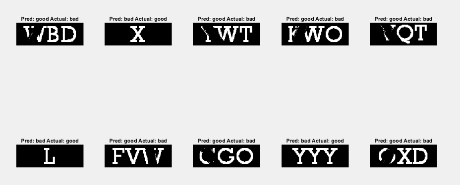
It was observed (as shown in Fig 4) that the rare cases of misclassification only included those BE samples where the blot occurred on a corner. (It may be noted that the training data consists of about 5000 BE samples and the misclassification occurred in less than 10 such cases in the worst of trials). An intuitive modification was to use non-square filters as the text is mostly dominated by prominently vertical and horizontal features while the ‘blots’ would not show such characterization. Proceeding on these lines, the 2 layers were then made to have 5X10 and 10X5 sized filters. This shot up the accuracy to more than 99.5%. It can be seen that the BE misclassification cases were eliminated virtually entirely (compare fig and fig).
Another observation that was drawn from Fig 4 was about the LSEs. It was noted (in multiple tests) that the misclassified LSEs were almost entirely dominated by artefacts that were solid (less fuzzy) and very vertical. Intuitively as well, it is an efficient way to blemish printed text. This was in part because there were relatively few solid, vertical LSEs (see section II-A). And because they blend excellently with the text making them harder to categorise. This caused us to tweak our algorithms to create more such artefacts for training. We made 1000 such errors and added them to our dataset. The result was as expected and all cases of such misclassification disappeared. Interesting thing to note from this expedition was that our methods (algorithms, per se) were malleable enough to specially accomodate any such special, pertinent, artefact which may sabotage the readability of the document.
The most unsurprising yet fascinating improvement was owed to Batch normalization [12]. Without it, both the training and testing performance were very incompetent and erratic. The best case accuracy was 89% which is practically unacceptable in our application. Even during training, the accuracy would fluctuate heavily across epochs.[19]
In our prior analysis, we briefly considered experimenting with asymmetric cost function in later stages of implementation [22]. This was synchronous with the practical expenses in implementation – the cost of printing few sheets of paper redundantly is much less than printing a single sheet which may be ambiguous to read. However, we did not implement it at any stage as the accuracy was very high. Even a slight asymmetry in classification would wreak havoc on the testing result. Since these networks analyse multiple text segments on a single sheet – which are typically in the range of 100 to 300 – the error per sheet would seriously increase in any such implementation. We do however hope to try it on other databases that might be available as more research in this field is published in public domain.

Our aim was to automate the print error detection process in a large scale printing press where data readability is of utmost importance. We evaluated multiple solutions and realised that ConvNets would be the most efficient and fast way to tackle this problem. We discussed the most pertinent categories of print errors and how can they be simulated. Our first major contribution was to create a public database [1] for such a problem which thus far, seemed unavailable. We then established how ConvNets proved to be the optimum solution because of thei speed, and a staggering accuracy of 99.83%. We analysed the heuristics in the implementation and training of network. Another intersting observation is that none of the erroneous images which were misclassified are ambiguos in reading. It shows that despite having a shallow architecure, the model learnt in part, a sense of ’readability’ rather than shear feature detection[23].
Our future work would be centred primarily around testing the results on real data and on different kinds of text data. Different text formats will have different features, thus our network may not be a panacea for the entire class of print error detection. Thus far we only worked on uncompressed images and only tested ConvNets.

References

- [1]
Print Error Database URL:
https://tinyurl.com/y677fhjz - [2] Ashia C Wilson, Rebecca Roelofs, Mitchell Stern, Nathan Srebro, and Benjamin Recht. The marginal value of adaptive gradient methods in machine learning. arXiv preprint arXiv:1705.08292, 2017.
- [3] A. M. Sabu and A. S. Das, ”A Survey on various Optical Character Recognition Techniques,” 2018 Conference on Emerging Devices and Smart Systems (ICEDSS), Tiruchengode, 2018, pp. 152-155. doi: 10.1109/ICEDSS.2018.8544323
- [4] J. Xie, ”Optical Character Recognition Based on Least Square Support Vector Machine,” 2009 Third International Symposium on Intelligent Information Technology Application, Shanghai, 2009, pp. 626-629. doi: 10.1109/IITA.2009.327
- [5] T. K. Hazra, D. P. Singh and N. Daga, ”Optical character recognition using KNN on custom image dataset,” 2017 8th Annual Industrial Automation and Electromechanical Engineering Conference (IEMECON), Bangkok, 2017, pp. 110-114. doi: 10.1109/IEMECON.2017.8079572
- [6] Shepanski, ”Fast learning in artificial neural systems: multilayer perceptron training using optimal estimation,” IEEE 1988 International Conference on Neural Networks, San Diego, CA, USA, 1988, pp. 465-472 vol.1. doi: 10.1109/ICNN.1988.23880.
- [7] R. Kozma, M. Kitamura, A. Malinowski and J. M. Zurada, ”On performance measures of artificial neural networks trained by structural learning algorithms,” Proceedings 1995 Second New Zealand International Two-Stream Conference on Artificial Neural Networks and Expert Systems, Dunedin, New Zealand, 1995, pp. 22-25. doi: 10.1109/ANNES.1995.499430
- [8] Hailong Jia and Kun Cao, ”The research on the preprocessing algorithm for fingerprint image,” 2012 IEEE Symposium on Electrical & Electronics Engineering (EEESYM), Kuala Lumpur, 2012, pp. 163-166. doi: 10.1109/EEESym.2012.6258614
- [9] V. Vasilyev, ”Structural design of shallow neural networks on the basis of minimal complexity principle,” 2016 24th Mediterranean Conference on Control and Automation (MED), Athens, 2016, pp. 1212-1217. doi: 10.1109/MED.2016.7535872
- [10] M. Bianchini and F. Scarselli, ”On the Complexity of Neural Network Classifiers: A Comparison Between Shallow and Deep Architectures,” in IEEE Transactions on Neural Networks and Learning Systems, vol. 25, no. 8, pp. 1553-1565, Aug. 2014. doi: 10.1109/TNNLS.2013.2293637
- [11] S. Noel and H. Szu, ”Multiple-resolution divide and conquer neural networks for large-scale TSP-like energy minimization problems,” Proceedings of International Conference on Neural Networks (ICNN’97), Houston, TX, USA, 1997, pp. 1278-1283 vol.2. doi: 10.1109/ICNN.1997.616218
- [12] V. Thakkar, S. Tewary and C. Chakraborty, ”Batch Normalization in Convolutional Neural Networks — A comparative study with CIFAR-10 data,” 2018 Fifth International Conference on Emerging Applications of Information Technology (EAIT), Kolkata, 2018, pp. 1-5. doi: 10.1109/EAIT.2018.8470438
- [13] Xu, B., Wang, N., Chen, T., Li, M., 2015. Empirical evaluation of rectified activations in convolutional network, arXiv preprint arXiv:1505.00853
- [14] Glorot, X., Bordes, A. & Bengio. Y. Deep sparse rectifier neural networks. In Proc. 14th International Conference on Artificial Intelligence and Statistics 315–323 (2011).
- [15] X. Qi, T. Wang and J. Liu, ”Comparison of Support Vector Machine and Softmax Classifiers in Computer Vision,” 2017 Second International Conference on Mechanical, Control and Computer Engineering (ICMCCE), Harbin, 2017, pp. 151-155.
- [16] Nasr, G. E., Badr, E. A., & Joun, C. (2002). Cross Entropy Error Function In Neural Networks: Forecasting Gasoline Demand. FLAIRS-02 Proceedings of the AAAI.
- [17] Dogo, E & Afolabi, O & I Nwulu, N & Twala, Bhekisipho & Aigbavboa, Clinton. (2018). A Comparative Analysis of Gradient Descent-Based Optimization Algorithms on Convolutional Neural Networks.
- [18] S. Ioffe and C. Szegedy. Batch normalization: Accelerating deep network training by reducing internal covariate shift. In ICML, 2015.
- [19] E. Phaisangittisagul, ”An Analysis of the Regularization Between L2 and Dropout in Single Hidden Layer Neural Network,” 2016 7th International Conference on Intelligent Systems, Modelling and Simulation (ISMS), Bangkok, 2016, pp. 174-179. doi: 10.1109/ISMS.2016.14
- [20] Srivastava, N., Hinton, G., Krizhevsky, A., Sutskever, I. & Salakhutdinov, R. Dropout: a simple way to prevent neural networks from overfitting. J. Machine Learning Res. 15, 1929–1958 (2014).
- [21] P. M. Radiuk, “Impact of training set batch size on the performance of convolutional neural networks for diverse datasets,” Information Technology and Management Science, vol. 20, no. 1, pp. 20–24, 2017.
- [22] S. F. Crone, ”Training artificial neural networks for time series prediction using asymmetric cost functions,” Proceedings of the 9th International Conference on Neural Information Processing, 2002. ICONIP ’02., Singapore, 2002, pp. 2374-2380 vol.5. doi: 10.1109/ICONIP.2002.1201919
- [23] Ba, Jimmy, and Rich Caruana. ”Do deep nets really need to be deep?.” Advances in neural information processing systems. 2014.
- [24] Smith R. An overview of the Tesseract OCR engine; Int. Conf. on Document Analysis and Recognition (ICDAR); 2007.