MPPI-VS: Sampling-Based Model Predictive Control Strategy for Constrained Image-Based and Position-Based Visual Servoing
Abstract
In this paper, we open up new avenues for visual servoing systems built upon the Path Integral (PI) optimal control theory, in which the non-linear partial differential equation (PDE) can be transformed into an expectation over all possible trajectories using the Feynman-Kac (FK) lemma. More precisely, we propose an MPPI-VS control strategy, a real-time and inversion-free control strategy on the basis of sampling-based model predictive control (namely, Model Predictive Path Integral (MPPI) control) algorithm, for both image-based, 3D point, and position-based visual servoing techniques, taking into account the system constraints (such as visibility, 3D, and control constraints) and parametric uncertainties associated with the robot and camera models as well as measurement noise. Contrary to classical visual servoing control schemes, our control strategy directly utilizes the approximation of the interaction matrix, without the need for estimating the interaction matrix inversion or performing the pseudo-inversion. We validate the MPPI-VS control strategy as well as the classical control schemes on a 6-DoF Cartesian robot with an eye-in-hand camera based on the utilization of four points in the image plane as visual features. To better assess and demonstrate the robustness and potential advantages of our proposed control strategy compared to classical schemes, intensive simulations under various operating conditions are carried out and then discussed. The obtained results demonstrate the effectiveness and capability of the proposed scheme in coping easily with the system constraints, as well as its robustness in the presence of large errors in camera parameters and measurements.
Multimedia Material
The supplementary video attached to this work is available at: https://bit.ly/3JrSJUu
I INTRODUCTION
Visual servoing, also known as vision-based control, has been widely used in robotics and automation society, providing more flexible and intelligent machines utilized in many applications such as assembly tasks [1], detection and tracking missions [2, 3, 4], surgical tasks [5], unmanned aerial vehicles [6], ultrasound probe guidance [7], welding [8], and spray painting [9]. Generally speaking, visual servoing refers to the use of computer vision data, acquired from one or several cameras, for controlling the motion of a robot. Typically, the camera has two fundamental configurations. First, it can be mounted directly on a robot (e.g., robot manipulator or mobile robot), where the robot motion produces the motion of the camera. Second, it can be fixed in the workspace, in order to observe the motion of the robot. The former configuration refers to eye-in-hand systems, whereas the latter indicates eye-to-hand systems. From the control schemes perspective, visual servoing can be typically classified into three categories: (i) image-based visual servoing (IBVS), in which the control law is directly based on the error between the current and desired image features on the 2D image plane; (ii) position-based visual servoing (PBVS), where the pose of the camera, relative to some reference coordinate frame, is computed to be used by the control law [10]; and (iii) hybrid visual servoing, in which, one way or another, a combination of IBVS and PBVS is utilized [11].
Generally, the IBVS control scheme has received much attention both in scientific literature and in industry-oriented research due to its inherent robustness against not only camera calibration imperfections but also against modelling errors [12], exhibiting better local stability and convergence properties. In contrast to PBVS control strategy that is often very sensitive to camera calibration errors, which lead to errors in the 3D reconstruction of the target object in the environment and accordingly errors during task execution. In addition, as the control law of PBVS is explicitly expressed in Cartesian space and there is apparently no direct control to the visual features on the image plane, these features or some may leave the camera’s field of view (FoV). Furthermore, compared with PBVS, IBVS does not require a perfect knowledge of the 3D model of the target, and only some information about the object depths are required. Nevertheless, there exist some issues associated with IBVS, which should be addressed, such as: (i) its convergence is theoretically constrained to a region around the desired camera pose; (ii) in some cases, singularities (or poor conditioning) in the interaction matrix11 1 In IBVS, the mapping between visual features velocities in image space and camera velocity in Cartesian space is encoded in the interaction matrix, which will be briefly discussed in Section II. and image local minima may occur, leading to control problems and probably spilling down the servoing task; (iii) since there is no direct control over the camera velocity in Cartesian space, as the control law is defined in the image plane, the executed trajectories by the robot, in the Cartesian space, could be quite contorted; (iv) other concern is the difficulty of constraints handling such as visibility constraints, which imposed by the fact that the visual features should constantly remain within the camera’s FoV. It is noteworthy that these major problems have been clearly pointed out in [13].
I-A Related Work
To this so, several control approaches have been proposed in the literature, so as to improve the visual servoing performance and overcome the previously highlighted difficulties. Just to name a few, the problem of image singularities could be solved by finding the suitable visual features of visual servoing, such as Cylindrical [14], Spherical [15], Polar [16] coordinate systems, and moment features [17]. A good alternative solution based on the task function approach is investigated in [18], for avoiding robot joint limits and kinematic singularities. While, in [19], several control schemes based on second-order minimization techniques have been conducted for avoiding the camera retreat problem (as introduced in [13]). In [20], the authors proposed a Takagi–Sugeno fuzzy framework for modelling the IBVS scheme, in which the singularity can be handled and the stability can be easily verified. Another improvement is achieved by so-called 2-1/2D visual servoing approach, which is one of the well-known hybrid schemes, where the characteristics of the IBVS and PBVS methods are combined [11]. Similarly, soon afterwards, authors in [21] proposed a new approach based on augmenting depth information within the visual features vector. While Thuilot et al. [22] proposed a new control strategy for PBVS in which an online trajectory is planned on the image plane in order to ensure that the object remains within the FoV. In addition, other hybrid or partitioned schemes have been developed based on (i) decoupling the translational camera motions from the rotational ones [23, 24, 25]; or (ii) switching either between different control schemes (i.e., IBVS and PBVS control schemes) [26, 27, 28] or between two different coordinate systems [29, 30]. For instance, Allibert and Courtial [29] proposed a switching control scheme for IBVS tasks based on Cartesian and Polar image coordinates, taking the advantages of both Cartesian- and Polar-based IBVS strategy. Other promising methods based on combining path planning and trajectory tracking were developed in the literature for coping with constraints handling (see, e.g., [31] and [32]).
Recently, model predictive control (MPC) strategies have been widely used in the related literature, with the aim of improving the quality of visual servoing and coping with constraints which have not been explicitly handled by most of the previously mentioned approaches. For example, an unconstrained stabilizing receding horizon control strategy is applied to 3D visual servoing [34], while other predictive control approaches have been proposed to deal with constraints in IBVS [35, 36, 37, 38, 39]. Particularly, in [35], an MPC-based approach is proposed for constraints handling and image prediction, demonstrating its robustness with respect to errors in the camera parameters and noise in the measured visual features. Nonetheless, no robustness (i.e., stability) analysis was performed, which has been lately addressed, e.g., in [36] and [39], and the controller has not been experimentally validated. Based on the polytopic transformation of the interaction matrix, a robust quasi-min-max MPC strategy was proposed in [37], which was also validated via simulation studies. The two proposed approaches in [35] and [37] suffer from the computational burden since solving the optimization problem exceeds the real system-sampling time (i.e., they are not implemented online). Sequentially, it can be quite difficult to be applied to the real system. In order to alleviate and tackle this problem, various methods have been developed to guarantee a real-time solving optimization problem such as in [40, 41, 42]. In [40], the authors utilized the primal-dual neural network (PDNN) as a promising computational tool for solving the quadratic programming (QP) problem and achieving a real-time implementation of MPC, instead of using the sequential quadratic programming (SQP) method which requires repeatedly a calculation of Hessian matrix to solve a QP problem [41]. Fusco et al. [42] presented a real-time IBVS prediction control scheme for a robotic arm based on integrating the acceleration of the visual features, which allows the controller to produce better input signals compared to classical predictive strategies.
On the other hand, a new algorithmic methodology based on Path Integral (PI) optimal control theory has recently been proposed by Kappen in [43], for solving the nonlinear Stochastic Optimal Control (SOC) problem. Traditionally, on the basis of dynamic programming, the SOC problem is defined by a partial differential equation (PDE) known as the Hamilton-Jacobi-Bellman (HJB) equation. More generally, this equation can not be solved analytically. On other words, it can only be solved numerically backward-in-time and, unfortunately, numerical solutions are intractable due to the curse of dimensionality [44]. This is actually one of the primary reasons for proposing a PI control theory, in which the non-linear PDE can be transformed into an expectation over all possible trajectories using the Feynman-Kac (FK) lemma. This transformation allows the SOC to be solved by sampling methods, such as forward-in-time Monte-Carlo approximation, instead of solving the HJB equation backward-in-time. Inspired by the PI control theory, Williams et al. [45] proposed a sampling-based model predictive control algorithm known as Model Predictive Path Integral (MPPI) control framework, which has been successfully applied to a variety of robotic systems for tasks such as aggressive autonomous driving and autonomous flying through 2D cluttered environments. More recently, a generic and elegant MPPI control framework has been presented in [46], which enables the robot to navigate autonomously in either 2D or 3D environments which are inherently uncertain and partially observable.
It is obviously sufficiently that both MPPI and MPC follow the same control strategy, which can be summarized as: (i) the optimal control action is obtained by solving, at each time step, a finite-horizon constrained optimization problem, considering the current state of the system to be controlled as the initial state; (ii) then, the optimization yields an optimal control sequence; (iii) finally, the first control in this sequence is applied to the system being controlled. However, we believe that the MPPI control framework significantly outperforms the conventional MPC strategy for the following reasons. First, since it is a sampling-based and derivative-free optimization method, it does not require the computation of gradients (i.e., derivatives) so as to find the optimal solution. As a consequence, it can be readily implemented online and applied to the real system. Second, it does not require the first- or second-order approximation of the system dynamics and quadratic approximation of the cost functions, i.e., highly non-linear and non-convex functions can be naturally utilized. Moreover, this flexibility also allows the dynamics to be easily represented by neural networks [47]. Third, its ability to cope with hard and soft constraints easily, making it so attractive in many robotics fields. Additionally, discontinuous cost functions, i.e., indicator functions, can be easily handled and added to the running cost function. For instance, in the context of autonomous flying tasks, a large-weighted indicator function can be employed as part of the running cost, for penalizing the collision with ground or obstacles. Forth, MPPI can still provide a reasonable solution when there exists no feasible solution, which (i.e., feasibility issue) represents one of the most predominant issues in MPC schemes that adds additional complexity to the optimization problem [48].
I-B Contributions
Motivated by the observations above, within this paper, we present the framework of PI control theory to the visual servoing systems. More precisely, we propose a real-time and inversion-free control method on the basis of the MPPI control framework for both image-based (IBVS), 3D point (3DVS), and position-based (PBVS) visual servoing control schemes, which has been validated on a 6-DoF Cartesian robot (namely, Gantry robot) with an eye-in-hand camera. We call this new approach the MPPI-VS control strategy. Consequently, the underlying goal of the work described in this paper is two-fold:
- 1.
examining the possibility of employing the MPPI control framework for visual servoing (VS) systems, particularly, in our case, for VS systems based on the utilization of four points in the image plane as visual features; to the best of the authors’ knowledge, this is the first attempt to develop a VS control strategy based on MPPI;
- 2.
highlighting its potential advantages for improving the quality of visual servoing, in terms of the image prediction, constraints handling, and overcoming other aforementioned difficulties as far as possible.
The major contributions of the work described in this paper can be summarized as follows:
- •
We propose a real-time sampling-based MPC algorithm for predicting the future behavior of the VS systems, without solving the online optimization problem which usually exceeds the real system-sampling time and suffers from the computational burden.
- •
No need for estimating the interaction matrix inversion or performing the pseudo-inversion in real-time [49]; our proposed MPPI-VS control strategy directly utilizes the approximate interaction matrix, i.e., it is an inversion-free control method.
- •
We also propose a direct estimation (i.e., online estimation) of 3D parameters (i.e., depth ) of the interaction matrix under the assumption that the initial object depths, , are known; on other words, no need for solving a set of linear equations using least-squares or using iterative updating schemes [50].
- •
The system constraints (namely, visibility, three-dimensional (i.e., 3D), and control constraints) and parametric uncertainties associated with the robot and camera models can be easily posed and handled.
- •
For IBVS, the proposed approach (so-called MPPI-IBVS) has the capability of tackling the camera retreat problem without proposing hybrid methods or decoupling the -axis motions from the others degrees of freedom [23], thanks to the prediction process which allows to explicitly enforce better behaviour of the camera’s motion.
- •
Finally, for PBVS, we propose two methods to ensure that the object always remains within the camera’s FoV since the control law is explicitly expressed in Cartesian space and there is no direct control to the visual features on the image plane.
This paper is an extension of our previously-published study in [33], with a more detailed explanation and analysis. As an improvement over the previous study, this article demonstrates in detail the intensive simulations jointly with a set of examples from the successful servoing tasks that shows the behavior of the proposed control strategy compared to the classical control schemes, including: (i) the trajectories in both the image and Cartesian space, (ii) the camera velocity components, and (iii) the visual features error (for instance, see Fig. 3). Moreover, it studies the convergence time of the proposed control schemes, as well as how the camera local minimum can be effectively avoided.
I-C Paper Organization
The rest of this paper is organized as follows. In Section II, we briefly recall the mathematical formulation of the classical IBVS, 3DVS, and PBVS control schemes for a pinhole camera model. Section III describes our proposed MPPI-VS control strategy, detailing how the system constraints can be handled, whereas Section IV is dedicated to the intensive simulation results and discussion. Finally, conclusions and future work are given in Section V.
II Classical Visual Servoing Control Schemes
Broadly speaking, the main objective of all vision-based control schemes is to minimize the error between the current visual features and the desired features , which is typically defined as
| (1) |
assuming, herein, that the camera observes stationary visual features (i.e., is constant) and any changes in depend only on the motion of the camera.

The global structure of both IBVS and PBVS control schemes, for a 6-DoF Grandy robot, is illustrated in Fig. 1. The main difference between these control schemes is in the way that is designed. More specifically, for IBVS control schemes, consists of a set of image features that expressed directly in the 2D image space; whilst for PBVS control schemes, it is composed of a set of 3D parameters that estimated from the visual features extracted from the image. In this section, we briefly recall the mathematical formulation of the classical IBVS, 3DVS, and PBVS (namely, C-IBVS, C-3DVS, and C-PBVS) control schemes for a pinhole camera model, considering only the utilization of a set of point-like features as visual features extracted from a 2D image.
II-A Image-Based Visual Servoing (IBVS)
Consider as coordinates of a 3D point feature expressed in the camera frame in meter units, which can be projected onto the image plane as a 2D image point feature with coordinates expressed in pixel units. Let be the spatial velocity of the camera in the world frame, composed of the linear velocities and the angular velocities . For the eye-in-hand configuration, the time derivative of the coordinates of point can be directly related to the camera velocity by
| (2) |
This equation can be written in the matrix form as
| (3) |
where refers to the interaction matrix related to the 3D point relative to the camera frame. Furthermore, according to the principle of a pinhole camera perspective projection, we can relate the normalized image-plane coordinates to the pixel coordinates using the well-known equation
| (4) |
where denotes the set of camera intrinsic parameters: , , is the camera focal length, are the horizontal and vertical dimension of a pixel, and are the coordinates of the principal point. Using (3) and (4), the relationship between the time variation of visual features and the camera velocity screw can be modeled as
| (5) |
where the interaction matrix (also called image Jacobian matrix) of a 2D point feature , with respect to the principal point, is given by
and in the interaction matrix denotes the depth of the feature point with respect to the camera frame. More details, concerning the derivations, can be found in [51].
The simplest and well-known control strategy to IBVS is to merely use (1) and (5) to construct the control law that drives the current features toward their desired values on the image plane. Thus, this classical feedback control law is given by
| (6) |
where denotes the pseudo-inverse of an estimation of , since it is impossible in practice to know exactly either or . In this work, the four well-known cases for constructing the approximate are considered and studied, to be used in both classical IBVS control strategy and our proposed one, which are as follows:
- 1.
CASE #0: ; in the present case, we assume that each visual feature and its depth are estimated at each iteration of the control scheme under the assumption that the initial depth of each point-like feature is known.
- 2.
CASE #1: ; herein, it is supposed that the feature points must be updated at each iteration, whereas the depth of each point is considered to be fixed and is set to the estimated value of at the desired camera position, i.e., .
- 3.
CASE #2: ; the simplest case is to consider the interaction matrix as a constant matrix with not only but with also . This means that no estimation will be carried out, at each iteration, during the visual servoing task, and only the desired depth of each point needs to be set.
- 4.
CASE #3: Finally, we considered the choice that has been proposed in [19], which relies on the use of the mean of the estimation of the interaction matrix at the current iteration (namely, CASE #0) and at equilibrium (namely, CASE #2); i.e., in this case, .
II-B Position-Based Visual Servoing (PBVS)
In the PBVS control strategy, the visual features extracted from the image are utilized for estimating the pose of the camera relative to either (i) a reference frame tied to the object, or (ii) the desired camera frame . Thus, can be generally defined as , where denotes a translation vector; whereas represents a rotation vector, where is a unit vector representing the rotation axis and is the rotation angle. Within this work, we define as the translation vector between the current camera frame and its desired frame . Therefore, the aim of the control scheme is to drive the camera so that converges to . As a result, we have , , and . Furthermore, by following the developments presented in [52], the interaction matrix relative to can be obtained by
| (8) |
where refers to the rotation matrix between frames and , and the Jacobian matrix is given by
| (9) |
in which denotes a identity matrix, is the skew-symmetric matrix associated with vector , and . Similar to IBVS scheme, the time derivative of can be related to the camera velocity screw by
| (10) |
Accordingly, we can obtain the simplest, i.e., classical, PBVS control strategy by
| (11) |
which can be decoupled into: , and , where .
III MPPI Control Strategy for Visual Servoing
In this section, we briefly present the control strategy of our proposed sampling-based MPC approach (namely, MPPI) for visual servoing systems; then, we state the mathematical formulation of MPPI in the presence of constraints such as the visibility, three-dimensional (i.e., 3D), and control constraints.
III-A Review of MPPI
The MPPI control strategy is a sampling-based and derivative-free optimization method to model predictive control (MPC) that can be easily applied in real-time (i.e., online) to the real system, without requiring the first- or second-order approximation of the system dynamics and quadratic approximation of the objective functions.
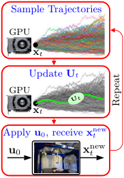
The real-time control cycle of MPPI is shown in Fig. 2. At each time-step , MPPI samples thousands of trajectories from the system dynamics (e.g., in our case, from Eq. (3), (5), or (10)), using a Graphics Processing Unit (GPU) so as to ensure a real-time implementation. Afterward, on the basis of the parallel nature of sampling, each of these trajectories is individually executed and then evaluated according to its expected cost. In sequential, the optimal control sequence , over a finite prediction time-horizon , is updated based on a weighted average cost over these generated trajectories, where , and refers to the number of timesteps. Finally, the first control is applied to the system, while the remaining control sequence of length is slid-down to be used for providing a warm-starting to the optimization at the next time-step.
Let be a zero-mean Gaussian noise vector with a variance of , i.e., , where represents the random noise associated with the commanded control input to the system; in other words, it represents the control input updates as the actual input is . Suppose that the number of the samples (namely, trajectories or rollouts) drawn from the discrete-time dynamics system, , is , where denotes the state of the system at time . Moreover, let be the cost-to-go of the trajectory from time onward. Then, based on the detailed derivation given in [45] and well-summarized in [46], the optimal control sequence can be readily updated using the following iterative update law:
| (12) |
where is so-called the inverse temperature which determines the level of the selectiveness of the weighted average. We defined the cost-to-go of each trajectory over the predefined prediction time-horizon as
| (13) |
in which refers to the terminal cost. Whilst denotes the instantaneous running cost, which composed of the sum of state-dependent running cost and quadratic control cost, and is defined as follows:
where is a positive definite control weight matrix, and is so-called the exploration noise which determines how aggressively MPPI explores the state-space; the impact of changing has been studied in [46].
III-B MPPI-VS Control Strategy
In order to apply the MPPI control strategy to the visual servoing systems, the non-linear discrete-time form of the continuous-time dynamical model given in (3), (5), or (10) is required, for simulating and propagating thousands of trajectories in parallel. This discrete-time model can be approximated using the Newton–Euler method as
| (14) |
whereby defines the state vector of the model (i.e., the MPPI states) at time instant , where (i) for MPPI-IBVS control scheme, the state vector refers to a set of 2D points, i.e. ; (ii) for MPPI-3DVS control scheme, it is composed of a set of 3D point features, i.e., ; while (iii) for MPPI-PBVS control scheme, the state vector is defined as , as described in Section II. Similarly, the approximate interaction matrix is given by either or for MPPI-IBVS, 3DVS, PBVS} control schemes, respectively. It is generally apparent that our MPPI-VS control strategy directly utilizes the estimation of the interaction matrix, without the need for estimating the interaction matrix inversion or performing the pseudo-inversion in real-time. Furthermore, it is noteworthy that for the MPPI-IBVS control scheme, particularly for CASE #0 and #3 of the approximate where the depth of each point-like feature needs to be estimated, we use the discrete-time model of the 3D point features given in (14) for predicting the future evolution of the object depths , assuming that, at each time-step , the initial depth of a set of point-like features is known.
III-B1 Handling Visibility and 3D Constraints
One of the most attractive features of MPPI, compared to the classical MPC, is its capability of coping easily with the hard and soft constraints, without adding additional complexity to the optimization problem. More precisely, a large-weighted indicator function can be employed as part of the state-dependent running cost function for handling the constraints. In our case, for MPPI-VS control scheme, the instantaneous state-dependent running cost function, , is defined as
| (15) |
where denotes the state-dependent cost which is a simple quadratic cost for enforcing the current state to reach its desired value .
On the other hand, refer to an indicator function utilized for handling:
- (i)
the visibility constraints to ensure that the visual features always remain within the image plane; they can be simply expressed as , where and refer to the lower and upper ranges, in pixels, of the image point coordinates, and
- (ii)
the three-dimensional (i.e., 3D) constraints such as workspace or joint limits; in the present work, we did not consider the joint limits as a part of the optimization problem, in order to better understand the behavior of MPPI whenever one of the joints reaches its given bounds. In practice, the joint limits are handled by the robot controller as illustrated in Fig. 1; thus, if the robot reaches the joint bounds, the velocity of each joint will be set to zero.
The definition of is mainly based on the MPPI-VS control scheme to be implemented. Therefore, in the MPPI-IBVS control scheme, is formulated as
| (16) |
where and are Boolean variables that are used to heavily penalize each trajectory that violates the visibility and 3D constraints, respectively. For instance, is turned on (i.e., ) if, at any time, exceeds its given bounds, i.e., . Since the joint limits have not been considered as a part of the MPPI optimization problem, we can add the second term, if needed, for constraining the future evolution of the 3D point features, namely, . Just to name a few, this term can be added for avoiding the camera retreat motion, which occurs when there is a large rotation between the initial and desired camera configuration (this phenomenon is known as the camera retreat problem), by simply penalizing the -axis translation motion of each 3D point feature relative to the camera frame. In the present case, will be active if at any time the depth of one point, at least, exceeds a threshold , where defines the maximum allowable camera retreat motion along its optical axis, i.e., .
In the MPPI-PBVS control scheme, the controller might produce control input that would ultimately leads to that some visual features may leave the camera’s FoV, just as in the classical PBVS control strategy expressed in (11). Sequentially, the pose of the object can not be estimated and, then, the robot will be stopped as the control loop is no longer closed. This is mainly due to the fact that the control law is explicitly expressed in Cartesian space and there is apparently no direct control to the visual features on the image plane. Therefore, we propose two methods so as to guarantee that the object always remains within the camera’s FoV. Concerning the first proposed method, the indicator function is defined as a large-weighted exponential penalty function, as follows:
| (17) |
so that the visibility constraints are constantly satisfied which can be written as , where denotes the normalized Cartesian coordinates of an image point, , are the minimum and maximum bounds, in meters, of the point feature projected on the normalized image plane, while and are positive scalar variables. In the second method, we proposed an alternative solution based on augmenting the 3D point features within the nominal state vector. In further words, we combine both MPPI-PBVS and MPPI-3DVS control schemes. Thus, in this case, we have , whilst . In the present scheme, the penalty (i.e., indicator) function is replaced by a large-weighted quadratic state-dependent cost function which modulates how fast the current state vector of the 3D point features converges to its desired one . Therefore, the running cost function , which is given in (15), is reformulated as
| (18) |
where , is the length of the state vector , whereas refer to the cost weighting of and , respectively. It should be noted that assigning very high weights, particularly for , is sufficient for enforcing the visual features to stay within the image plane, without imposing additional constraints on the optimization problem.
III-B2 Handling Control Constraints
Most robotic systems, including the 6-DoF Cartesian robot we consider here, have constraints on the actuators, such as range or velocity limitations, that must be taken into consideration in the control law design. These constraints are known as control constraints which considered to be hard constraints that should not be violated. In the case of MPPI control strategy, there exist two ways for handling the control constraints. First, they can be implemented as a natural part of the running cost by adding an appropriate term (e.g., indicator function), as we previously explained, to penalize all the trajectories that violate the constraints. However, the common issue associated with this way is that the control constraints acting as soft constraints, and, accordingly, it is notoriously difficult to ensure that the control input, obtained by the controller, remains always within its allowed bounds, even after rejecting each trajectory that violates the control input limits. Therefore, within this work, we utilize an alternative method based on pushing the control constraints into the dynamics system [47], meaning that , where is an element-wise clamping function that is used to restrict the control input to remain within a given range, for all samples drawn from the dynamics system. Thus, can be defined as , where and are the lower and upper bounds of the control input. The major advantage, here, is that the problem formulation of MPPI, which takes into account control constraints, is converted into an unconstrained one, without violating the constraints and affecting the convergence of the MPPI algorithm as has an impact only on the dynamics system.
IV Simulation-Based Evaluation
In the present section, we conduct extensive simulations on a simulated 6-DOF Cartesian robot with an eye-in-hand camera configuration so as to evaluate and demonstrate the potential advantages of our proposed control strategy for improving the quality of visual servoing tasks, along with a comparison to the classical schemes (namely, C-IBVS, C-3DVS, and C-PBVS schemes).
IV-A Simulation Settings and Performance Metrics
We validated the MPPI-VS control strategy as well as the classical schemes on a 6-DOF Cartesian robot (namely, Gantry robot) based on the utilization of four points (i.e., ) in the image plane as visual features.22 2 The reason behind choosing the Cartesian robot is that it has a quite large workspace that helps to verify the robustness of the MPPI-VS control scheme. For more information about the real robot simulator: https://visp.inria.fr/robot-interface/ & https://github.com/lagadic/visp_ros/blob/master/nodes/afma6.cpp During all the simulations, it is assumed that the MPPI algorithm runs with a time horizon of , a control frequency of (i.e., ), and generates samples each time-step with an exploration variance of . Moreover, the control weighting matrix is set to , assuming that the random noise associated with the control input has a variance of . On the other side, the remaining parameters, which needed to be adjusted on the basis of the MPPI-VS scheme to be implemented, are tabulated in Table I, as well as the camera intrinsic parameters. More concretely, in the case of MPPI-IBVS scheme, it can be noticeable that the inverse temperature is set to a higher value. Conversely, it is tuned to much lower values in both MPPI-3DVS and MPPI-PBVS control schemes. It is important to bear in mind that fine-tuning is mainly based on the state-dependent running cost function and in which plane (i.e., 2D image plane or Cartesian plane) it is expressed. The real-time MPPI-VS algorithm is executed on an NVIDIA GeForce GTX 1080 Ti desktop GPU. In addition, all the control schemes, including the classical ones, were developed in Python and C++ and were implemented using Visual Servoing Platform (ViSP) [53] integrated with the Robot Operating System (ROS) framework.
| Parameter | Value | Parameter | Value |
|---|---|---|---|
| Camera Intrinsic Parameters | |||
| Image Res. [] | [] | ||
| [] | [] | ||
| [] | [] | ||
| Parameters of MPPI-IBVS Control Scheme | |||
| Parameters of MPPI-3DVS Control Scheme | |||
| Parameters of MPPI-PBVS Control Scheme | |||
| (17) | , | (18) | , |
IV-A1 Initial Camera Configurations
To better assess and demonstrate the robustness level of our proposed control strategy, initial camera configurations were randomly extracted from a uniform distribution within the robot’s workspace, with a guarantee that (i) the robot kinematics has initially the capability of reaching these generated poses, and (ii) the visual features are initially located within the camera’s FoV. The four point-like features were located in the -plane at the positions , , and [] (see Fig. 3(b)).
IV-A2 Desired Camera Configurations
In this work, we considered two different desired poses of the camera, all expressed in the reference frame attached to the object with -axis pointing downward. The first desired camera pose was chosen along the -axis with a translation vector [], heading toward the features with an orientation vector []. Hence, the desired coordinates of the four points in the image plane are , where , , , and []; meaning that the object lies in the center of the image, as illustrated in Fig. 3. We have defined the second camera configuration in such a way that the features are much closer to the edge of the camera’s FoV (i.e., the object is located near one of the image borders), to demonstrate how robust the proposed control strategy is against violating the system constraints particularly visibility constraints. Herein, the camera pose relative to the object frame is set to in ([], []). As a result, the object lies in the top-right corner of the image.
IV-A3 Performance Metrics
For each initial camera configuration, we considered the following. First, for the conventional VS control schemes, the simulation is run for on a realistic simulator of the real robot. Whereas for our proposed MPPI-VS scheme, we adopted the simulation time to be as it is noticed that the convergence rate is empirically slow, especially in the case of MPPI-IBVS scheme, as will be discussed later. Second, the visual servoing task is considered to be successful if the following are satisfied:
- (i)
The camera does not reach a local minimum (which indicated as or False, during the simulations). Such configuration corresponding to a local minimum occurs when and . Mathematically, we utilized the mean-squared error (MSE) as a metric that measures the positioning error , which can be formulated as in which and . Thence, we considered that the local minimum is completely avoided (i.e., ) if and only if and , where (in []) and (in []) refer to the translational and rotational errors between and , respectively. During the simulations, we set the two thresholds as and .
- (ii)
The robot joint limits are avoided (i.e., ). If the robot reaches one of the joint limits, the velocity of each joint will be set to zero by the robot controller (for safety reasons) and, accordingly, will be turned to 1.
- (iii)
The visual features (in our case, the four points) always remain within the camera’s FoV (i.e., ). Furthermore, in the experimental validation, it has been assumed that the robot will immediately stop as soon as one of the features is no longer visible in the image.
Finally, the number of successful servoing tasks, with respect to the total initial camera configurations, is denoted as , while indicates the success rate.
IV-B Intensive Simulation Details and Results
In order to validate the theoretical findings and emphasize the efficiency of the MPPI-VS control strategy, intensive simulation studies have been performed under various operating conditions, with the aim of (i) highlighting the potential advantages of our proposed strategy for improving the performance of visual servoing in terms of visual features prediction and constraints handling, (ii) fine-tuning the parameters of the MPPI algorithm and, then, studying the impact of changing these parameters as they play a critical role in determining the robustness and ensuring the convergence of the algorithm, and (iii) studying the influence of both modeling errors (e.g., errors in camera calibration and depth estimation) and measurement noises on the visual servoing.
| Test No. | Control Scheme | |||||
|---|---|---|---|---|---|---|
| MPPI-IBVS and C-IBVS Control Schemes | ||||||
| Test #1 | MPPI- (CASE #0) | 0 | 0 | 1 | 119 | 99.16% |
| Test #2 | MPPI- (CASE #1) | 0 | 0 | 29 | 91 | 75.8% |
| Test #3 | MPPI- (CASE #2) | 0 | 0 | 54 | 66 | 55% |
| Test #4 | MPPI- (CASE #3) | 0 | 0 | 6 | 114 | 95% |
| Test #5 | MPPI- (CASE #0) | 0 | 0 | 0 | 120 | 100% |
| Test #6 | C- (CASE #0) | 0 | 0 | 37 | 83 | 69.17% |
| Test #7 | C- (CASE #0) | 0 | 0 | 36 | 84 | 70% |
| Test #8 | MPPI- (CASE #0) | 0 | 0 | 19 | 101 | 84.17% |
| Test #9 | MPPI- (CASE #0) | 0 | 0 | 35 | 85 | 70.8% |
| Test #10 | MPPI- (CASE #0) | 0 | 0 | 7 | 113 | 94.17% |
| Test #11 | MPPI- (CASE #0) | 0 | 0 | 15 | 105 | 87.5% |
| Test #12 | MPPI- (CASE #0) | 0 | 0 | 25 | 95 | 79.17% |
| Test #13 | C- (CASE #0) | 0 | 0 | 42 | 78 | 65% |
| Test #14 | MPPI- (CASE #0) | 0 | 0 | 0 | 120 | 100% |
| Test #15 | MPPI- (CASE #0) | 0 | 0 | 2 | 118 | 98.33% |
| Test #16 | MPPI- (CASE #0) | 0 | 0 | 5 | 115 | 95.83% |
| Test #17 | MPPI- (CASE #0) | 0 | 0 | 17 | 103 | 85.83% |
| Test #18 | MPPI- (CASE #0) | 0 | 0 | 4 | 116 | 96.67% |
| MPPI-3DVS and C-3DVS Control Schemes | ||||||
| Test #19 | MPPI- () | 0 | 0 | 0 | 120 | 100% |
| Test #20 | C- ( | 0 | 0 | 4 | 116 | 96.67% |
| Test #21 | MPPI- () | 0 | 0 | 5 | 115 | 95.83% |
| Test #22 | C- () | 0 | 1 | 6 | 113 | 94.17% |
| MPPI-PBVS and C-PBVS Control Schemes | ||||||
| Test #23 | MPPI- () | 0 | 45 | 0 | 75 | 62.50% |
| Test #24 | C- () | 0 | 26 | 0 | 94 | 78.33% |
| Test #25 | C- () | 0 | 22 | 0 | 98 | 81.17% |
| Test #26 | MPPI (, (17)) | 0 | 0 | 0 | 120 | 100% |
| Test #27 | MPPI (, (17)) | 0 | 0 | 0 | 120 | 100% |
| Test #28 | MPPI (, (18)) | 0 | 0 | 0 | 120 | 100% |
Table II summarizes the overall performance of each control scheme individually, given the initial camera configurations. In total, we conduct a set of different tests. The first tests, included in the intensive studies, focus on studying the quality and robustness of both MPPI-IBVS and C-IBVS control schemes, while the remaining tests assess the performance of MPPI-3DVS and MPPI-PBVS compared to C-3DVS and C-PBVS control schemes. Furthermore, the simulations are carried out considering as the desired camera configuration (unless mentioned otherwise, i.e., ).
IV-B1 Prediction Process Influence
In the first four tests (namely, from Test #1 to #4), we analyzed the impact of the image prediction process on the performance of the MPPI-IBVS control strategy taken into account the four cases of the approximate interaction matrix , that have been previously discussed in Section II-A, and the MPPI-IBVS parameters listed in Table I. It can be clearly seen that the prediction process exerts a high influence as MPPI provides better performance in CASE #0 and #3, in which the 2D visual features and their depth information are assumed to be estimated each iteration. While the worst performance is achieved when is assumed to be constant, as depicted in Test #3. More accurately, for Test #1, we conducted trials. For all the trials, our proposed control scheme succeeded in completing out of tasks/configurations (i.e., ), while there existed only one initial camera configuration led the robot to reach one of its joint limits (i.e., ). It is noteworthy that this one failure case can be readily tackled by increasing the prediction horizon as illustrated in Test #5 where we adopted and instead of and , showing the superiority of our proposed control strategy even without involving the robot joint limits in the prediction algorithm. Moreover, is decreased to half of its nominal value so as to ensure a real-time implementation of MPPI-IBVS, without compromising its robustness level and convergence rate.
IV-B2 C-IBVS Control Scheme
To better understand the potential advantages of MPPI-IBVS in improving the performance of visual servoing, intensive simulations of the classical IBVS control scheme are carried out in Test #6 and #7 in which we set to and , respectively.
As anticipated, the success rate of visual servoing tasks was reduced to , with - failure cases. In fact, these failure cases occurred due to the fact that their corresponding initial camera configurations have large rotations around the camera optical axis as well as their positions along the -axis are much closer to the minimum allowable limit of the third joint which is approximately relative to the object reference frame . Thus, thanks to the prediction process, it has been possible to provide better camera trajectories without violating the robot joint bounds. In Fig. 3, we illustrate the behavior of MPPI-IBVS compared to C-IBVS through an example from the successful servoing tasks (namely, task #113) in both Tests #1 and #6. We can observe that despite the trajectories of the four points in the image are less satisfactory than those obtained from C-IBVS, our proposed control scheme provides a smooth trajectory of the camera in the Cartesian space (see Figs. 3(a) and 3(b)), with very low fluctuations in the camera velocity components as depicted in Fig. 3(c). Furthermore, it is worthy to notice that MPPI-IBVS ensures convergence in both the image and 3D space as in C-IBVS; however, the convergence of the image points is no longer perfectly exponential (see Fig. 3(e)). Herein, the system converges within approximately (or, 991 iterations) compared to (or, 723 iterations) in the case of C-IBVS.
IV-B3 MPPI Parameters Influence
In Tests #1 and #5, we have clearly seen that fine-tuning the parameters of MPPI plays an important role in determining its behavior and improving the quality of positioning tasks. As a consequence, the boundary of the workspace and joint limits have been avoided during the servoing operation. Therefore, in the next three tests starting from Test #8, the influence of both control input updates , prediction horizon , and number of sampled trajectories is individually studied. In Test #8, we adopted , while in Test #9 is set to . Finally, we set to in Test #10. In general, the intensive simulations demonstrate that the impact of either having short-time horizons or changing the control input updates is appreciably higher than the influence of decreasing the number of samples , as the success rate in Tests #8 and #9 is significantly lower than that in Test #10. Concerning the quality of successful servoing tasks, it is interesting to notice that assigning very low values to and affects the convergence rate33 3 Notice that the simulation time of Test #9 is adopted to be as the convergence rate of MPPI, in this case, is extremely slow. and quality of the trajectories in both the image and 3D space. Just to name a few, for the positioning task #113 given in Fig. 3, the system converges to its desired pose within about with , instead of taking in case of .
IV-B4 Handling Control and 3D Constraints
In Test #11, we repeated the simulations of Test #1 under the assumption that the maximum control input of the camera velocity screw is limited to for the translational speed and for the rotational speed, while the minimum control input equals to . Broadly speaking, we can observe that restricting the control input affects the overall performance of MPPI-IBVS, particularly for those camera configurations that require large motions especially, in our simulations, those containing large rotations around -axis. Within the present test, the - failure cases can be easily avoided and tackled by involving the 3D constraints, especially joint limits constraints, as a part of the MPPI-IBVS optimization problem. On the other side, the obtained results of the successful tasks demonstrate that our proposed control scheme performs perfectly with a high capability of handling the control constraints.
Figure 4 shows the behavior of MPPI-IBVS for servoing task #45; in such a configuration, C-IBVS fails as the third joint reaches its allowable lower limit due to the large translational and rotational motions. As can be clearly seen in Fig. 4(a), the trajectories of the point-like features in the image in the constrained case are almost similar to that in the unconstrained case. The corresponding translational and rotational motions of the camera expressed in are given in Fig. 4(b). We can notice that the camera converges to the desired camera configuration with: (i) translational errors less than in both - and -directions and less than in the -direction, and (ii) rotational errors less than (i.e., ). It is also interesting to observe that the lower limit of the third joint is reached, as in C-IBVS, at . Accordingly, the robot controller set the joints’ velocities to zero (see the gray highlighted region in Fig. 4(b)). Nevertheless, our proposed control scheme has the capability of getting out of it at , due to the stochastic nature of the optimal control sequence obtained by the MPPI algorithm that mainly based on a stochastic sampling of system trajectories. Finally, Figs. 4(c) and 4(d) display the constrained and unconstrained optimal control input of the camera velocity screw . It is observed that the clamping function that is used to restrict the control input is only applied to the component (see Fig. 4(c)) since its value exceeds the given bound which is (see Fig. 4(d)), while the remaining components of the camera velocity behave almost the same with unnoticeable changes.
Apart from the intensive simulations, we considered another servoing task, in which the camera performs a pure rotation of about its optical axis44 4 Notice that the maximum allowable rotational motion of our Cartesian robot around -axis (i.e., camera optical axis) is approximately expressed in the object frame ., as an example to illustrate the 3D constraints handling and how the camera retreat motion can be avoided as previously discussed in Section III-B. In such a configuration, both C-IBVS and unconstrained MPPI-IBVS (with CASE #0) got stuck in the lower limit of the third joint due to the camera retreat motion. However, once we set the maximum allowable camera retreat motion to with respect to , the constrained MPPI-IBVS algorithm has the capability of converging easily to the desired camera configuration by penalizing the -axis translation motion of each 3D point as illustrated in Figs. 5(a)-5(c), without violating the control constraints (see Fig. 5(d)).
IV-B5 Handling Visibility Constraints
In all tests where MPPI-IBVS is utilized, the simulations are carried out taken into account the visibility constraints, which are defined by the following inequalities:
| (19) |
Additionally, in order to better evaluate its capability of handling the constraints, the simulations of Test #1 are repeated in Test #12, considering as the desired configuration instead of . The intensive simulations presented in Table II demonstrate the efficiency and capability of our proposed control strategy in coping easily with the visibility constraints, as the visual features always remain within the camera’s FoV (i.e., for all tests).
Two positioning tasks from Test #12 are displayed in Fig. 6, illustrating the superiority of MPPI-IBVS although one of the features is initially located (i) on the border of the image (see in Fig. 6(a)) or (ii) near the border with large rotation along the optical axis (see in Fig. 6(b)). The initial camera configurations of tasks #12 and #100 are and in ([], []), respectively. Moreover, in Test #13, we repeated the simulations of C-IBVS given in Test #6 with respect to , not . We can clearly observe that the failure cases increased owing to the complex translational and rotational motions associated with , compared to ; one of the failure cases is task #100, while C-IBVS converges to the desired pose in task #12, as shown in Fig. 6.
IV-B6 MPPI-IBVS Robustness
To test the robustness of our proposed control strategy with respect to camera modeling errors and measurement noise, a set of intensive simulations has been considered in the next five tests. More precisely, in Test #14, a white noise generated from a uniform distribution is added to the visual features and their 3D information (i.e., depth estimation) with a maximum error of for 2D features and for 3D points. The influence of having a and error in the camera’s focal length is individually investigated in Tests #15 and #16, respectively, whereas in Test #17 we considered the case that combines various errors in the camera intrinsic parameters : in , in , in , in , and in . Finally, the simulations carried out in Test #18 take into consideration both the added measurement noise and camera calibration error given in Tests #14 and #15.


As can be seen in Table II, our proposed control scheme behaves perfectly as there exists a maximum of - failure cases that occurred in Test #17, demonstrating its robustness in the presence of large errors in camera parameters and measurements, in addition to ensuring the convergence of the system.
Figure 7 demonstrates a comparison between the behavior of MPPI-IBVS and C-IBVS in terms of the measurement noise described in Test #14. We can observe that MPPI-IBVS follows almost exactly the same trajectories in the image, while it provides a bit long camera trajectory compared to the nominal case with very low fluctuations in the camera velocity components, as illustrated in Figs. 7(a), 7(b), and 7(c). On the other side, in the case of C-IBVS, in spite of both the points’ and 3D camera trajectories follow almost straight lines, the visual servoing is unstable due to high oscillations in the camera velocity components produced by the classical control law (see Fig. 7(d)). Figures 7(e) to 7(h) show the evolution of the error of both image features and 3D points for the two control schemes, as well as their corresponding error norm . It should noticed that the maximum steady-state features error norm, for both schemes, is less than which is significantly lower than the added noise, while the steady-state 3D points error norm is mainly centered around .
In Fig. 8, we present the behavior of both control schemes with respect to camera calibration errors. As can be seen in Figs. 8(a) and 8(b), the behavior of our proposed control scheme in Cartesian space is more satisfactory than that of C-IBVS, especially in the case where the combined errors are considered (namely, Test #17). Furthermore, the more interesting property is that those calibration errors have no remarkable effect on both: (i) the followed trajectories in the image (see Fig. 8(c)), (ii) the quality of optimal control input of the camera velocity screw as illustrated in Fig. 8(e), and (iii) the convergence rate (see Fig. 8(g)). In practice, this clearly means that MPPI-IBVS is largely compatible with a rough calibration (i.e., no need for an accurate calibration step), with sustaining a wide margin of the overall stability of the system. In addition, concerning C-IBVS, it can be seen in Figs. 8(b) and 8(d) that neither the 3D camera trajectory nor the image points trajectories follow straight lines owning to bad calibration, which might increase the possibility of the visual features leaving the camera’s FoV. Sequentially, the evolution of the error is no longer perfectly exponential (see Fig. 8(h)).
Figure 9 demonstrates the robustness of our proposed control scheme with respect to a bad estimation of the object depths , starting from having an offset of (i.e., half the true value) and ending with an offset of (i.e. three times the true value). Moreover, the obtained results clearly demonstrate the fact that MPPI-VS does not require an accurate mathematical model of the system dynamics; i.e., in our case, an approximate interaction matrix is sufficient to compute the optimal control sequence.
IV-B7 3DVS Control Schemes
In this work, 3DVS has been mainly utilized by the MPPI algorithm either for predicting the future evolution of the object depths at each iteration in case of MPPI-IBVS or for coping with the visibility constraints of MPPI-PBVS as previously described in (18). Nevertheless, four intensive simulations are carried out in Tests #19 to #22 for assessing the performance of both MPPI-3DVS and C-3DVS (with , considering the two desired camera configurations and the MPPI-3DVS parameters listed in Table I. The simulations show that both control strategies give very satisfactory results, where the maximum failure cases were ( for and only one for ) occurred in Test #22. Figure 10 gives an example illustrating the behavior of both control schemes. Despite the 2D features in case of MPPI-3DVS follow more complex trajectories compared to that in MPPI-IBVS (see Figs. 10(a) and 3(a)), the fluctuations of the camera velocity components and the evolution of the error are significantly lower (where lower is better) in the steady-state, as can be seen in Figs. 10(c) and 10(e). While C-3DVS provides almost straight-line trajectories in the image and 3D space as in C-IBVS.

IV-B8 Unconstrained MPPI-PBVS V.S. C-PBVS
In the last six tests, intensive simulations are conducted to verify the performance of our proposed PBVS control scheme. In the first three tests (namely, from Test #23 to #25), we studied the behavior of MPPI-PBVS without applying the visibility constraints, together with the performance of the classical scheme. The obtained results demonstrate that both control strategies produce control input ultimately leading to that some visual features leave the camera’s FoV (i.e., ). Moreover, it is interesting to notice that (i) C-PBVS provides more satisfactory results than MPPI-PBVS as our proposed scheme has in total - failure cases, in which at least one point leaves the FoV, compared to a total of - cases obtained by C-PBVS in Test #24, and (ii) the robot joint limits are totally avoided (i.e., there exist no- failure cases).
IV-B9 Constrained MPPI-PBVS
Now, it is the time to assess the performance of MPPI-PBVS taken into consideration the two methods proposed in (17) and (18) to cope with the visibility constraints. Tests from #26 to #28 demonstrate the validness and effectiveness of our proposed methods in handling visibility constraints, regardless of which desired camera configuration is considered (i.e., whether or ), as there exist neither nor failure cases.
Figure 11 illustrates the behavior of MPPI-PBVS based on (17) and (18) for the servoing task #15. In such a configuration, only C-IBVS successfully fulfills the servoing task as the four points always remain in the image as shown in Fig. 11(a), while it is observed that the unconstrained MPPI-PBVS that presented in Test #23 causes failure of servoing since three points leave the image (namely, , and ). However, the visibility constraints have been respected, once one of our proposed methods is involved in the MPPI algorithm as the visual features have been forced to stay in the image (see again Fig. 11(a)). It is also observed that despite MPPI-PBVS on the basis of (18) provides better motion in the image space, the 3D camera trajectory obtained by applying (17) is considerably shorter than that obtained by applying (18), as illustrated in Fig. 11(b). It is noteworthy that the quality of trajectories obtained by (18), particularly in the image plane, and satisfying the visibility constraints are mainly based on the assigned value to the cost weighting of particularly , as previously discussed in Section III-B. The impact of changing on the performance of MPPI-PBVS is studied in Table III. It can be clearly noticed that by assigning low values to , our control scheme is unable to constantly satisfying the visibility constraints. For instance, if is assigned to instead of (the value we have set during our intensive simulations), three points will leave the FoV (i.e., ). Thus, the higher this value, the better the performance. For this reason, it is highly recommended to utilize (17) in the prediction algorithm as the constraints have not been violated.
| 1 | 3 | 2 | 2 | 5 | 1 |
| 10 | 1 | 20 | None | 50 | None |
Figures 11(c) and 11(d) show the evolution of the six components of the camera velocity for the constrained MPPI-PBVS based on (17) and C-PBVS, while the evolution of the error of the camera pose relative to the desired camera frame is shown in Fig. 11(f). We can notice that our control scheme achieves a slightly faster convergence; the system converges to the desired configuration within compared to when C-PBVS is used. Furthermore, its behavior in the steady state is roughly similar to that of MPPI-3DVS and, once again, better than that of MPPI-IBVS. Finally, the evolution of the camera pose with respect to the object reference frame is shown in Fig. 11(e). It is quite interesting to observe that the positioning error precision obtained in this servoing task is less than for the translation and for the rotation.
IV-B10 Reaching Local Minimum
Concerning all tests where MPPI is deployed, it should be clearly observed from Table II that the controller performs perfectly without the camera reaching a local minimum (i.e., for all tests). We noticed during our intensive simulations that the most significant parameter for avoiding reaching a local minimum or crossing a singularity of the interaction matrix is the inverse temperature , as determines how tightly peaked the optimal distribution is. In other words, for instance, in the case of MPPI-IBVS, we observed that low values of result in many trajectories being rejected due to their costs are too high. In addition, low values lead to empirically slow convergence to the desired configuration, with a slightly fluctuating motion of the camera.
IV-B11 MPPI-VS Convergence Time
To quantitatively evaluate the performance of the convergence of our proposed control schemes, the index of the convergence time of the successful servoing tasks is first utilized; then, Gaussian distribution of those successful tasks was fitted with a histogram plot as shown in Fig. 12. The convergence is considered to be achieved if the error norm is less than for MPPI-IBVS and for both MPPI-3DVS and MPPI-PBVS.
Figures 12(a) and 12(b) show the histogram of the convergence time of MPPI-IBVS for three conducted trials of Test #1 and the four cases of that previously discussed in Section II-A. From the three trials, we can infer that the majority of those tasks converge to the desired camera configuration within approximately . Moreover, as anticipated, the average convergence time of MPPI-IBVS considering both CASE #0 and #3 is quite shorter than that of CASE #1 and #2, thanks to the estimation of the visual features and their depth information.
In Figs. 12(c) and 12(d), we present the histograms of the convergence time of our proposed control schemes compared to the classical schemes. We can clearly observe that the convergence time of MPPI-PBVS is remarkably shorter (with very low standard deviation) than that of MPPI-IBVS and classical schemes. This relates to the fact that the control law given in (12) and the state vector of the former control strategy are expressed in the same space (i.e., Cartesian space), while the state vector and, sequentially, the state-dependent running cost function of the latter strategy are expressed in the image plane which results in a slightly low convergence to the desired camera configuration. Furthermore, the standard deviation in the case of MPPI-IBVS is quite large since, in some particular configurations, the controller got stuck in the robot joints’ limits for few seconds before reaching the desired pose, as previously discussed in Fig 4.
V Conclusion and future work
In this work, a real-time sampling-based MPC strategy (so-called MPPI-VS) has been successfully developed for predicting the future behavior of the visual servoing systems such as IBVS, 3DVS, and PBVS control schemes, without solving the online optimization problem which usually exceeds the real system-sampling time and suffers from the computational burden. This control strategy leverages the approximate interaction matrix; i.e., there is no need for estimating the interaction matrix inversion or performing the pseudo-inversion. Our proposed control strategy, as well as the classical control strategies, has been successfully tested on realistic and intensive simulations via a 6-DoF Cartesian robot with an eye-in-hand camera configuration. Through those intensive studies, it is demonstrated that MPPI-VS has the following properties. First, it has the capability of coping easily with both hard and soft constraints including visibility, 3D, and control constraints, without adding additional complexity to the optimization problem. Second, contrary to classical IBVS, it is highly robust against not only the uncertainties associated with the robot and camera models but also against the measurement noise of the visual features. Finally, for PBVS, it ensures that the object always remains within the camera’s FoV and, also, ensures a faster convergence rate to the desired pose, compared to other proposed schemes. Our future work will be devoted to experiments on a real robot. Moreover, the possibility of running the MPPI algorithm on CPUs will be investigated, instead of using GPUs, with the aim of reducing the computational burden.
Declarations
Funding
This work was supported by the French ANR CLARA (ANR-18-CE33-0004), Université Côte d’Azur, INRIA Sophia Antipolis, France.
Acknowledgements
The author would like to thank Guillaume Allibert, Philippe Martinet, Fabien Spindler, Ezio Malis, and Lantao Liu for their assistance and valuable comments.
References
- [1] B. Hamner, S. Koterba, J. Shi, R. Simmons, and S. Singh, “An autonomous mobile manipulator for assembly tasks,” Autonomous Robots, vol. 28, no. 1, pp. 131–149, 2010.
- [2] S. Minaeian, J. Liu, and Y.-J. Son, “Vision-based target detection and localization via a team of cooperative UAV and UGVs,” IEEE Transactions on systems, man, and cybernetics: systems, vol. 46, no. 7, pp. 1005–1016, 2015.
- [3] Y. Qiu, B. Li, W. Shi, and X. Zhang, “Visual servo tracking of wheeled mobile robots with unknown extrinsic parameters,” IEEE Transactions on Industrial Electronics, vol. 66, no. 11, pp. 8600–8609, 2019.
- [4] T. P. do Nascimento, G. F. Basso, C. E. Dórea, and L. M. G. Gonçalves, “Perception-driven motion control based on stochastic nonlinear model predictive controllers,” IEEE/ASME Transactions on Mechatronics, vol. 24, no. 4, pp. 1751–1762, 2019.
- [5] M. Azizian, M. Khoshnam, N. Najmaei, and R. V. Patel, “Visual servoing in medical robotics: a survey. Part I: endoscopic and direct vision imaging–techniques and applications,” The international journal of medical robotics and computer assisted surgery, vol. 10, no. 3, pp. 263–274, 2014.
- [6] P. Serra, R. Cunha, T. Hamel, D. Cabecinhas, and C. Silvestre, “Landing of a quadrotor on a moving target using dynamic image-based visual servo control,” IEEE Transactions on Robotics, vol. 32, no. 6, pp. 1524–1535, 2016.
- [7] R. Mebarki, A. Krupa, and F. Chaumette, “2-D ultrasound probe complete guidance by visual servoing using image moments,” IEEE Transactions on Robotics, vol. 26, no. 2, pp. 296–306, 2010.
- [8] L. Zhou, T. Lin, and S.-B. Chen, “Autonomous acquisition of seam coordinates for arc welding robot based on visual servoing,” Journal of Intelligent and Robotic Systems, vol. 47, no. 3, pp. 239–255, 2006.
- [9] R. Chen, G. Wang, J. Zhao, J. Xu, and K. Chen, “Fringe pattern based plane-to-plane visual servoing for robotic spray path planning,” IEEE/ASME Transactions on Mechatronics, vol. 23, no. 3, pp. 1083–1091, 2017.
- [10] S. Hutchinson, G. D. Hager, and P. I. Corke, “A tutorial on visual servo control,” IEEE transactions on robotics and automation, vol. 12, no. 5, pp. 651–670, 1996.
- [11] E. Malis, F. Chaumette, and S. Boudet, “2 1/2 D visual servoing,” IEEE Transactions on Robotics and Automation, vol. 15, no. 2, pp. 238–250, 1999.
- [12] B. Espiau, “Effect of camera calibration errors on visual servoing in robotics,” in The 3rd International Symposium on Experimental Robotics III, Kyoto, Japan, Oct. 1993, pp. 182–192.
- [13] F. Chaumette, “Potential problems of stability and convergence in image-based and position-based visual servoing,” in The confluence of vision and control. Lecture Notes in Control and Information Sciences, D. J. Kriegma, G. D. Hager, and A. S. Morse, Eds. London: Springer, 1998, vol. 237, p. 66–78.
- [14] M. Iwatsuki and N. Okiyama, “A new formulation of visual servoing based on cylindrical coordinate system with shiftable origin,” in IEEE/RSJ International Conference on Intelligent Robots and Systems, vol. 1, Lausanne, Switzerland, Sept. 2002, pp. 354–359.
- [15] R. T. Fomena and F. Chaumette, “Improvements on visual servoing from spherical targets using a spherical projection model,” IEEE Transactions on Robotics, vol. 25, no. 4, pp. 874–886, 2009.
- [16] S. Liu and J. Dong, “Robust online model predictive control for image-based visual servoing in polar coordinates,” Transactions of the Institute of Measurement and Control, vol. 42, no. 4, pp. 890–903, 2020.
- [17] F. Chaumette, “Image moments: a general and useful set of features for visual servoing,” IEEE Transactions on Robotics, vol. 20, no. 4, pp. 713–723, 2004.
- [18] E. Marchand, F. Chaumette, and A. Rizzo, “Using the task function approach to avoid robot joint limits and kinematic singularities in visual servoing,” in IEEE/RSJ International Conference on Intelligent Robots and Systems, vol. 3, Osaka, Japan, Nov. 1996, pp. 1083–1090.
- [19] E. Malis, “Improving vision-based control using efficient second-order minimization techniques,” in IEEE International Conference on Robotics and Automation, vol. 2, New Orleans, LA, USA, Apr. 2004, pp. 1843–1848.
- [20] I. Siradjuddin, L. Behera, T. M. McGinnity, and S. Coleman, “Image-based visual servoing of a 7-DOF robot manipulator using an adaptive distributed fuzzy PD controller,” IEEE/ASME Transactions On Mechatronics, vol. 19, no. 2, pp. 512–523, 2013.
- [21] E. Cervera and P. Martinet, “Combining pixel and depth information in image-based visual servoing,” in 9th International Conference on Advanced Robotics, Tokyo, Japan, Oct. 1999, pp. 445–450.
- [22] B. Thuilot, P. Martinet, L. Cordesses, and J. Gallice, “Position based visual servoing: keeping the object in the field of vision,” in IEEE International Conference on Robotics and Automation, Washington, DC, USA, May 2002, pp. 1624–1629.
- [23] P. I. Corke and S. A. Hutchinson, “A new partitioned approach to image-based visual servo control,” IEEE Transactions on Robotics and Automation, vol. 17, no. 4, pp. 507–515, 2001.
- [24] O. Tahri, Y. Mezouar, F. Chaumette, and P. Corke, “Decoupled image-based visual servoing for cameras obeying the unified projection model,” IEEE Transactions on Robotics, vol. 26, no. 4, pp. 684–697, 2010.
- [25] D. Xu, J. Lu, P. Wang, Z. Zhang, and Z. Liang, “Partially decoupled image-based visual servoing using different sensitive features,” IEEE Transactions on Systems, Man, and Cybernetics: Systems, vol. 47, no. 8, pp. 2233–2243, 2017.
- [26] N. R. Gans and S. A. Hutchinson, “An asymptotically stable switched system visual controller for eye in hand robots,” in IEEE/RSJ International Conference on Intelligent Robots and Systems, vol. 1, Las Vegas, NV, USA, Oct. 2003, pp. 735–742.
- [27] G. Chesi, K. Hashimoto, D. Prattichizzo, and A. Vicino, “Keeping features in the field of view in eye-in-hand visual servoing: A switching approach,” IEEE Transactions on Robotics, vol. 20, no. 5, pp. 908–914, 2004.
- [28] N. R. Gans and S. A. Hutchinson, “Stable visual servoing through hybrid switched-system control,” IEEE Transactions on Robotics, vol. 23, no. 3, pp. 530–540, 2007.
- [29] G. Allibert and E. Courtial, “Switching controller for efficient IBVS,” in IEEE/RSJ International Conference on Intelligent Robots and Systems, Vilamoura, Portugal, Oct. 2012, pp. 1695–1701.
- [30] G. Ye, W. Li, H. Wan, and H. Lou, “Novel two-stage hybrid IBVS controller combining cartesian and polar based methods,” in IEEE International Conference on Mechatronics and Automation, Beijing, China, Aug. 2015, pp. 397–402.
- [31] M. Kazemi, K. Gupta, and M. Mehrandezh, “Path-planning for visual servoing: A review and issues,” in Visual Servoing via Advanced Numerical Methods. Lecture Notes in Control and Information Sciences, G. Chesi and K. Hashimoto, Eds. London: Springer, 2010, vol. 401, pp. 189–207.
- [32] D. Zheng, H. Wang, W. Chen, and Y. Wang, “Planning and tracking in image space for image-based visual servoing of a quadrotor,” IEEE Transactions on Industrial Electronics, vol. 65, no. 4, pp. 3376–3385, 2017.
- [33] I. S. Mohamed, G. Allibert, and P. Martinet, “Sampling-based mpc for constrained vision based control,” in 2021 IEEE/RSJ International Conference on Intelligent Robots and Systems (IROS). IEEE, pp. 3753–3758.
- [34] T. Murao, T. Yamada, and M. Fujita, “Predictive visual feedback control with eye-in-hand system via stabilizing receding horizon approach,” in Proceedings of the 45th IEEE Conference on Decision and Control, San Diego, CA, USA, Dec. 2006, pp. 1758–1763.
- [35] G. Allibert, E. Courtial, and F. Chaumette, “Predictive control for constrained image-based visual servoing,” IEEE Transactions on Robotics, vol. 26, no. 5, pp. 933–939, 2010.
- [36] S. Heshmati-Alamdari, G. K. Karavas, A. Eqtami, M. Drossakis, and K. J. Kyriakopoulos, “Robustness analysis of model predictive control for constrained image-based visual servoing,” in IEEE International Conference on Robotics and Automation, Hong Kong, China, May 2014, pp. 4469–4474.
- [37] T. Wang, W. Xie, G. Liu, and Y. Zhao, “Quasi-min-max model predictive control for image-based visual servoing with tensor product model transformation,” Asian Journal of Control, vol. 17, no. 2, pp. 402–416, 2015.
- [38] Z. Qiu, S. Hu, and X. Liang, “Model predictive control for constrained image-based visual servoing in uncalibrated environments,” Asian Journal of Control, vol. 21, no. 2, pp. 783–799, 2019.
- [39] P. Roque, E. Bin, P. Dos Santos Miraldo, and D. V. Dimarogonas, “Fast model predictive image-based visual servoing for quadrotors,” in IEEE/RSJ International Conference on Intelligent Robots and Systems, Las Vegas, NV, USA, Oct. 2020.
- [40] F. Ke, Z. Li, H. Xiao, and X. Zhang, “Visual servoing of constrained mobile robots based on model predictive control,” IEEE Transactions on Systems, Man, and Cybernetics: Systems, vol. 47, no. 7, pp. 1428–1438, 2017.
- [41] A. Hajiloo, M. Keshmiri, W.-F. Xie, and T.-T. Wang, “Robust online model predictive control for a constrained image-based visual servoing,” IEEE Transactions on Industrial Electronics, vol. 63, no. 4, pp. 2242–2250, 2015.
- [42] F. Fusco, O. Kermorgant, and P. Martinet, “Integrating features acceleration in visual predictive control,” IEEE Robotics and Automation Letters, vol. 5, no. 4, pp. 5197–5204, 2020.
- [43] H. J. Kappen, “Path integrals and symmetry breaking for optimal control theory,” Journal of statistical mechanics: theory and experiment, vol. 2005, no. 11, p. P11011, 2005.
- [44] B. Oksendal, Stochastic differential equations: an introduction with applications. Springer Science & Business Media, 2013.
- [45] G. Williams, A. Aldrich, and E. A. Theodorou, “Model predictive path integral control: From theory to parallel computation,” Journal of Guidance, Control, and Dynamics, vol. 40, no. 2, pp. 344–357, 2017.
- [46] I. S. Mohamed, G. Allibert, and P. Martinet, “Model predictive path integral control framework for partially observable navigation: A quadrotor case study,” in International Conference on Control, Automation, Robotics and Vision, Shenzhen, China, Dec. 2020, pp. 196–203.
- [47] G. Williams, N. Wagener, B. Goldfain, P. Drews, J. M. Rehg, B. Boots, and E. A. Theodorou, “Information theoretic MPC for model-based reinforcement learning,” in IEEE International Conference on Robotics and Automation, Singapore, May 2017, pp. 1714–1721.
- [48] D. Q. Mayne, J. B. Rawlings, C. V. Rao, and P. O. Scokaert, “Constrained model predictive control: Stability and optimality,” Automatica, vol. 36, no. 6, pp. 789–814, 2000.
- [49] J.-T. Lapresté, F. Jurie, M. Dhome, and F. Chaumette, “An efficient method to compute the inverse jacobian matrix in visual servoing,” in IEEE International Conference on Robotics and Automation, New Orleans, LA, USA, May 2004.
- [50] J. A. Piepmeier, G. V. McMurray, and H. Lipkin, “Uncalibrated dynamic visual servoing,” IEEE Transactions on Robotics and Automation, vol. 20, no. 1, pp. 143–147, 2004.
- [51] P. Corke, “Robotics, vision and control: fundamental algorithms in MATLAB,” in Springer Tracts in Advanced Robotics, 1st ed. Berlin Heidelberg: Springer-Verlag, 2011, vol. 73.
- [52] F. Chaumette and S. Hutchinson, “Visual servo control, part I: Basic approaches [tutorial],” IEEE Robotics & Automation Magazine, vol. 13, no. 4, pp. 82–90, 2006.
- [53] É. Marchand, F. Spindler, and F. Chaumette, “ViSP for visual servoing: a generic software platform with a wide class of robot control skills,” IEEE Robotics & Automation Magazine, vol. 12, no. 4, pp. 40–52, 2005.