Modelling uncertainty in financial tail risk: a forecast combination and weighted quantile approach
Abstract
A novel forecast combination and weighted quantile based tail-risk forecasting framework is proposed, aiming to reduce the impact of modelling uncertainty in tail-risk forecasting. The proposed approach is based on a two-step estimation procedure. The first step involves the combination of Value-at-Risk (VaR) forecasts at a grid of quantile levels. A range of parametric and semi-parametric models is selected as the model universe in the forecast combination procedure. The quantile forecast combination weights are estimated by optimizing the quantile loss. In the second step, the Expected Shortfall (ES) is computed as a weighted average of combined quantiles. The quantiles weighting structure for ES forecasting is determined by minimizing a strictly consistent joint VaR and ES loss function of the Fissler-Ziegel class. The proposed framework is applied to six stock market indices and its forecasting performance is compared to each individual model in the universe, a simple average approach and a weighted quantile approach. The forecasting results support the proposed framework.
Keywords: Value-at-Risk, Expected Shortfall, forecast combination, weighted quantile, quantile loss, joint loss.
JEL codes: C22, C58, G17.
1 Introduction
Since the introduction by J.P. Morgan in the RiskMetrics model in 1993, Value-at-Risk (VaR) has been widely employed by financial institutions and corporations around the world to assist their decision making in relation to capital allocation and risk management. VaR is a quantitative tool to measure and control financial risk and represents the market risk as one number. VaR has become a standard measurement for capital allocation and risk management. Let be the information available at time and
be the Cumulative Distribution Function (CDF) of return conditional on . We assume that is strictly increasing and continuous on the real line . Under this assumption, the level VaR (quantile) at time can be defined as:
However, VaR has been subject to criticism because it cannot measure the expected loss for violations and is not mathematically coherent, in that it can favor non-diversification. Expected Shortfall (ES), proposed by Artzner 1997 and Artzner et al. 1999, gives the expected loss, conditional on returns exceeding a VaR threshold, and is a coherent measure; thus, in recent years it has become more widely employed for tail risk measurement and is now favored by the Basel Committee on Banking Supervision. Within the same framework as above, the level ES can be shown to be equal to the tail conditional expectation of (see Acerbi and Tasche 2002, among others):
| (1) |
The Basel III Accord, which was implemented in 2019, places new emphasis on ES. Its recommendations for market risk management are illustrated in the 2019 document Minimum Capital Requirements for Market Risk that says: “ES must be computed on a daily basis for the bank-wide internal models to determine market risk capital requirements. ES must also be computed on a daily basis for each trading desk that uses the internal models approach (IMA).” (Basel Committee on Banking Supervision 2019, p. 89). According to the same document, when calculating ES banks must refer to the average loss in the tail below the 2.5% quantile level. Therefore, in the empirical application of our paper, we focus on one-step-ahead tail risk forecasting at the quantile level. In order to simplify notation, in the remainder, unless differently specified, the following notational conventions are adopted: and , where denotes the target 2.5% level for the estimation of VaR and ES.
Forecasts of VaR and ES can be generated through a variety of different models. Some of these, such as completely specified GARCH models, are fully parametric since they rely on the exact specification of the conditional distribution of returns and of the volatility dynamics. Differently, semi-parametric approaches require specific assumptions on the risk dynamics but without a return distribution assumption. Semi-parametric models can be applied to generate forecasts of VaR alone, that is the case of the conditional autoregressive VaR (CAViaR) models proposed by Engle and Manganelli 2004, or joint forecasts of the pair (VaR, ES). A joint semi-parametric model that directly estimates both VaR and ES, referred to here as the ES-CAViaR model, is proposed by Taylor 2019. Through incorporating an Asymmetric Laplace (AL) distribution with a time-varying scale, a quasi-likelihood can be built to enable the joint estimation of the conditional VaR and conditional ES in this framework.
Fissler and Ziegel 2016 develop a family of joint loss functions (or “scoring rules”) for the associated VaR and ES series that are strictly consistent for the pair (VaR, ES), that is, they are uniquely minimized by the true VaR and ES series. Applying specific choices of functions in the class of joint loss functions of Fissler and Ziegel 2016, it can be shown that such a loss function is exactly the same as the negative of the AL log-likelihood function presented in Taylor 2019. Patton et al. 2019 propose new dynamic models for VaR and ES, through adopting the generalized autoregressive score (GAS) framework (Creal et al. 2013 and Harvey 2013) and utilizing the loss functions in Fissler and Ziegel 2016.
Alternatively, a variety of semi-parametric approaches to the prediction of VaR and ES can be obtained by combining Quasi Maximum Likelihood (QML) estimation of the volatility coefficients with some non-parametric estimator of the error quantiles. Widely diffused and effective solutions rely on extreme value theory results, such as in the peaks-over-threshold approach (Gilli et al. 2006).
Storti and Wang 2021 have recently proposed a new ES estimation and forecasting framework, referred to as the Weighted Quantile (WQ) approach, where the ES is modelled as weighted average of tail quantiles. The quantiles are produced from the CAViaR model of Engle and Manganelli 2004 by grid search of a range of equally spaced quantile levels below the target VaR level, i.e., 2.5%. An advantage of this approach is that it sensibly reduces the impact of model uncertainty in the prediction of ES, that is modelled according to its natural definition as an average of tail quantiles. However, the specification of the optimal dynamic model for each quantile level is still subject to uncertainty. In order to limit the impact of the overall model uncertainty on the generation of joint (VaR, ES) forecasts, the WQ framework could actually be extended by replacing forecasts of tail quantiles from a single CAViaR model, as in Storti and Wang 2021, with forecast combinations from an ensemble of different models, of a possibly heterogeneous nature, that includes parametric as well as semi-parametric models. Then the ES forecasts could be generated as weighted averages of “combined” VaR predictors at different levels, employing the WQ framework.
The main motivation for this extension of the WQ framework relies on the consideration that, given the values of conditional tail quantiles, the ES is theoretically defined as the expectation of these quantiles. So, it can be immediately recognized that most of the modelling uncertainty is related to the modelling of tail quantiles, which will be addressed in this paper. The only residual uncertainty affecting ES estimation is potentially related to the identification of the grid of tail quantiles. However, as extensively discussed in Storti and Wang 2021, the ES estimates obtained through the WQ approach are not particularly sensitive to the selection of these hyper-parameters.
Aim of this paper is then to propose a novel approach to forecast VaR and ES based on Forecast Combination and Weighted Quantile (FC-WQ) techniques. The proposed framework can be treated as a generalization of the WQ framework proposed by Storti and Wang 2021 and its effectiveness is investigated through applications to stock market data, where direct comparisons between the FC-WQ and WQ approaches are conducted.
The paper is structured as follows. A review of strictly consistent scoring functions for joint estimation of VaR and ES is conducted in Section 2. Section 3 presents the the proposed approach and discusses its technical implementation details. The selected model universe for forecast combination is shown in Section 4. The results of an empirical application to real stock market data are presented and discussed in Section 5. Finally, Section 6 concludes.
2 Strictly consistent scoring functions for joint estimation of VaR and ES
From the main definition of ES provided in Equation (1), it follows that that is related to by the following integral
| (2) |
that, after a simple change of variable, can be rewritten as
| (3) |
In the literature, several alternative parameterizations of and have been proposed. The involved parameters can be consistently estimated from real data by minimizing appropriately chosen strictly consistent scoring functions. If the interest is solely in the estimation of VaR, the unknown coefficients in the dynamic specification of can be estimated by quantile regression mimizing the expected quantile loss function
with , where is the indicator function taking value 1 if event occurs and 0 otherwise, for .
Koenker and Machado 1999 show that the quantile regression estimator is equivalent to a maximum likelihood estimator when assuming that the data are conditionally distributed as an AL with a mode at the quantile of interest. If is the return on day and , then the parameters in the model for can be estimated by maximizing a quasi-likelihood based on:
for and where is a scale parameter.
Taylor 2019 extends this result to incorporate the associated ES quantity into the likelihood expression, noting a link between and a dynamic , resulting in the conditional density function:
| (4) |
This allows a likelihood function to be built and maximised, given model expressions for . In Equation (4), is the daily return, and denote the target level VaR and ES on day . Taylor 2019 notes that the negative logarithm of the resulting likelihood function is strictly consistent for considered jointly, i.e., it fits into the class of jointly consistent scoring functions for VaR and ES developed by Fissler and Ziegel 2016.
Members of this family are strictly consistent for , i.e., their expectations are uniquely minimized by the true VaR and ES series. The general form of this functional family is:
| (5) | |||||
where is increasing, is strictly increasing and strictly convex, and and is a real-valued integrable function.
As discussed in Taylor 2019, assuming to have zero mean, making the choices: , , and , which satisfy the required criteria, returns the scoring function:
| (6) |
Taylor 2019 refers to Equation (6) as the AL log score, which is a strictly consistent scoring function whose expectation is jointly minimized by the true VaR and ES series. The negative of Equation (6) equals to the log of Equation (4) and can be treated as the AL log-likelihood.
3 Proposed framework
3.1 The weighted quantile framework
In the Weighted Quantile (WQ) framework, level ES forecasts from a given model are generated in two steps. In step 1, given a grid of quantile levels of size , , with , an ensemble of VaR forecasts () is produced. In their empirical application Storti and Wang 2021 use CAViaR models for the modelling of tail quantiles. However, it is worth remarking that any model, parametric or semi-parametric, could be used to generate VaR forecasts for any . In principle, even different models, parametric and semi-parametric, could be used to fit quantiles at different levels. This feature makes the WQ framework highly flexible and adaptive.
In step 2, ES forecasts are then computed as an affine function of the tail quantile forecasts at levels as in Equation (7):
| (7) |
where the weights , , are generated by some flexible and parsimonious function, such as the Beta function. Namely, for , we have with
| (8) |
The main reasons for adopting the Beta specification to model the weights behaviour in Equation (7) are its parsimony, since it only depends on two parameters, and flexibility. However, as discussed in Storti and Wang 2021, other parameterizations are feasible and, in particular, for sufficiently low values of , the weights can be easily estimated individually as “free” parameters.
The intercept is estimated along with the other parameters and allows to correct biases potentially arising from the left truncation in the chosen grid of tail quantiles, thus further increasing the flexibility of the WQ approach.
Given first stage VaR forecasts, the unknown coefficients in Equation (7) are estimated by optimizing some strictly consistent scoring function such as the AL (Taylor 2019) or some other strictly consistent scoring function in the Fissler-Ziegel class.
3.2 A unified framework encompassing Forecast Combination and Weighted Quantile estimation
It is important to note that model uncertainty mainly affects step 1 of the WQ procedure, since the estimation formula used in step 2 naturally stems from the mathematical definition of ES as a function of the tail VaRs. In step 1 of the procedure, different models could result in being optimal for different quantile levels. On the other hand, in step 2, the ES is estimated applying its natural definition as expectation of the tail quantiles. The only residual source of modelling uncertainty is related to the selection of the grid of tail quantiles used for estimation in Equation (7) and, in particular, to the choice of the lower bound and of the value of . The impact of the choice of the lower bound is, by construction, controlled by the intercept and by the data driven weighting structure of the ES estimator, as also documented empirically by Storti and Wang 2021. Regarding the choice of , given the high computing power routinely available even on standard personal computers, implementing the WQ approach with a high value of , that virtually eliminates the discretization error, is not an issue and could be easily done while still keeping the computing time at reasonable levels. On the other hand, Storti and Wang 2021 show, by simulations and applications to real data, that the WQ gives remarkably good performances even for values of as low as 3 and that negligible improvements, in terms of forecasting accuracy, are expected from an increase in .
These considerations motivate a two-step approach based on a Forecast Combination and Weighted Quantile (FC-WQ) strategy, that is the main contribution of this paper. The technical details on the implementation of the two steps of the FC-WQ procedure are presented as below.
Step 1: Assume that different VaR forecasting methods are available and that each of them is fitted to generate series of VaR forecasts for a set of strictly increasing quantile orders . To be consistent with the standard regulatory prescription, we will focus on the case .
Letting be the length of the in-sample window and the length of the full-sample returns series, for each available model in our model universe ( models in total), VaR forecasts series will be generated from each model:
| (9) |
for , and where is the length of the out-of-sample period to be used for forecast evaluation. Overall, this will yield a total of series of VaR forecasts. For the -th model and -th quantile level, the generic -th one-step-ahead forecast () will be based on the model fitted to observations from to . Forecast combination is then used as a technique for reducing model uncertainty in VaR forecasting, yielding the combined quantile predictor that takes the general form
| (10) |
Therefore, in step 1, VaR forecasts from different models are combined to generate a set of “combined” VaR predictors at different quantile levels. In order to overcome the potential quantile crossing problem, the monotonization method proposed by Chernozhukov et al. 2010 is employed.
The framework in (10) can be in principle extended to consider non-linear combination schemes. This possibility is however not investigated in this paper. The proposed framework is highly flexible and can employ any model that could produce VaR estimates and forecasts, such as GARCH (Bollerslev 1986), CAViaR, etc. Details of the model universe will be presented in Section 4.
Step 2: In step 2, employing the WQ approach, the conditional ES at time is modelled as the weighted average of the combined quantiles from step 1:
| (11) |
where the weights , , are generated by a Beta weight function as in Equation (8)11 1 Following the implementation of WQ in (Storti and Wang 2021), we set the number of grid points equal to , so that the weight of the -quantile is not 0 by construction when using the Beta weight function to parameterize the weights pattern..
The combination of joint forecasts of VaR and ES has so far received scarce attention in the literature. The only contribution in this field is, to the extent of our knowledge, given by the paper of Taylor 2020 whose approach is however structurally different from the one that is taken in this paper. First, Taylor 2020 optimizes an AL loss function to combine joint (VaR,ES) models at a given target level , while our approach uses richer information on quantile levels falling in the tail of the distribution below . Second, our model universe is composed of VaR models rather than of joint (VaR, ES) models.
The next section focuses on the estimation strategy followed to estimate the , for , and the intercept term in step 1, and the (,,) coefficients in step 2.
3.3 Implementation of the FC-WQ predictor: estimation procedure
Next, we provide a detailed description of the estimation procedures implemented in the two steps of the proposed FC-WQ framework.
Estimation Step 1:
Under step 1, given the target quantile level , an equally spaced grid of quantile levels of size is selected,
where , with and , for . The value of the lower bound is selected as 0.005 and is selected as 3 and 5 in this paper, according to the findings in Storti and Wang 2021. For example, with and , fixing we have and the grid of quantile levels as .
Now, for each trial quantile level , individual models are employed to produce the () time series of conditional in-sample quantiles and the 1st one-step-ahead quantile forecasts , for and . The set of in-sample quantiles (produced from in-sample data from to or ) for models and at all trial quantile levels, from to , is collected in the array .
In our paper, a rolling window forecasting scheme is adopted, with as the length of the full-sample returns series. Therefore, for each step in the out-of-sample periods (still for each trial quantile level ), individual models are employed to produce the time series of one-step-ahead quantile forecasts , for and . This set of out-of-sample quantiles for models at all trial quantile levels is collected in the array , here .
Concatenating the two matrices (including in-sample quantile estimates) and (including one-step-ahead out-of-sample quantile forecasts) produces our quantile universe which is an array of size . The component of including in-sample VaR estimates and out-of-sample VaR forecasts at quantile level will be denoted as , that is a matrix.
The matrix and the series of returns are then given as input to the estimation procedure for VaR “combination” weights. Namely, as in Giacomini and Komunjer 2005, for a given VaR level and a forecast origin , the coefficients used for combining VaR forecasts at time , for (to include the intercept term ) can be estimated by minimizing the quantile loss function over a rolling window of fixed size
| (12) | ||||
where , (a vector of size , from row in matrix ), (a vector of size ), , for each quantile level , . Analytically, the estimated coefficients for combining one-step-ahead VaR forecasts with origin at time are given by
| (13) |
Combined one-step-ahead VaR forecasts are then finally computed through substituting the fitted coefficients in Equation (10)
| (14) |
Step 1 of the FC-WQ generates an output matrix of combined quantile predictors of size . Each column in this matrix is produced from combining conditional quantile estimates/forecasts from models. Namely, the values in column and rows from to in the matrix contain the 2.5% target level one-step-ahead quantile forecasts , noting .
Rows from 1 to are computed by estimating the combination weights on the in-sample quantile estimates from the candidate models and then using these weights to combine the time series of in-sample quantile estimates. The same weights, based on in-sample VaR estimates from time to , are used to generate row of the matrix. Row is then generated using weights estimated on the time series composed of in-sample quantile estimates from time to (for the first rows), and by the formerly generated vector of quantile forecasts at time (for the last row). This procedure is iterated, in a rolling window fashion, until the end of the available sample . A detailed step-by-step implementation description is shown in the Algorithm 1 presented after the illustration of the estimation step 2.
Estimation step 2:
In the second stage of our approach, we predict the conditional ES at time as an affine function of the elements of (row in matrix ). The only unknown parameters in Equation (11) for calculating the estimator are . Conditioning on first stage produced VaR series (a vector of size , row in matrix ) and letting , the values of the coefficients used for generating the ES forecast at time can be estimated by minimizing wrt the strictly consistent scoring function:
where
and
| (15) |
with (a vector of size ) and . is the quantile input at the target quantile level and produced from the estimation step 1 (row , column in matrix ).
Namely, the estimated coefficients for weighting the one-step-ahead combined VaR forecasts for time are obtained as
| (16) |
where . Minimization of the above AL log-score was implemented using the Quasi-Newton optimizer implemented in the Matlab fminunc function.
The estimated parameters and are plugged in the Beta lag function (8) to produce . Therefore, the fitted coefficients
| (17) |
are then employed in the weighted quantile framework as below to produce the -th one-step-ahead ES forecast at the target quantile level
| (18) |
For the sake of clarity, the detailed step by step description of the outlined forecasting algorithm is presented in Algorithm 1.
4 The model universe
Various types of models, such as parametric and semi-parametric VaR models, are selected as candidate models in the model universe. All these models, except for the CAViaR (Engle and Manganelli 2004), can be also used to generate ES forecasts. These ES forecasts will not be of interest for the implementation of the FC-WQ procedure but will be later used as benchmarks for ES forecasts comparison. In total, different models are selected with details shown below.
GJR-GARCH-t (parametric): the GJR-GARCH model, proposed by Glosten et al. 1993, extends the parametric GARCH model to capture the well-known leverage effect (negative returns at time have a larger impact on the volatility at time than positive returns). In addition, to capture the fat-tail property of financial returns, the Student-t distribution is employed.
EGARCH-t (parametric): as another commonly used parametric model, the EGARCH model (Nelson 1991) is also included as a candidate model. The EGARCH model does not require any positivity restriction on the parameters, since its volatility equation is on log-variance instead of variance itself. Thus the positivity of the variance is automatically satisfied, which is an important advantage of the framework. Again, the Student-t distribution is used to describe the potential leptokurtosis of the conditional return distribution.
POT-GJR-GARCH-t (semi-parametric): we also consider some semi-parametric models as part of the model universe. The peaks-over-threshold (POT)-GJR-GARCH-t combines the GJR-GARCH-t model with an extreme value theory (McNeil and Frey 2000) approach to the fitting of the tail properties of the error distribution. Namely, this is accomplished by applying the POT approach to the returns standardized by the GJR-GARCH-t estimated volatility; see Gilli et al. 2006 for details.
POT-EGARCH-t (semi-parametric): this approach is similar to the above described POT-GJR-GARCH-t with the difference that the POT method is applied to returns standardized by the EGARCH-t estimated volatility.
GJR-GARCH-t-HS (semi-parametric): a semi-parametric filtered historical simulation approach, which could potentially produce improved tail risk forecasting results, is also included. The series of in-sample conditional variance () is estimated based on the fitted GJR-GARCH-t model. The error quantiles and tail expectations are then estimated by computing the relevant sample quantiles and tail averages of standardized returns . Finally, level- VaR and ES forecasts are obtained by multiplying and , respectively, by the forecast from the fitted GJR-GARCH-t model.
EGARCH-t-HS (semi-parametric): this approach employs a similar procedure as the GJR-GARCH-t-HS, by replacing GJR-GARCH-t with EGARCH-t for volatility estimation and forecasting.
We would like to emphasise that, for the above models which rely on parametric volatility estimates and forecasts, we do not need to re-estimate the model for each trial quantile level ; , regarding the VaR and ES calculation. Differently, the remaining two models rely on direct modelling of VaR dynamics. Therefore, they need to be re-estimated for each trial quantile level .
CAViaR-AS (semi-parametric): the CAViaR models proposed by Engle and Manganelli 2004 are estimated using quantile regression. Although the CAViaR framework does not directly produce ES estimates and forecasts, it can be used without any issues in our FC-WQ approach which only requires the quantile estimates and forecasts from individual models.
Since the CAViaR model is used as the quantile estimation model in the WQ framework of Storti and Wang 2021, we have deliberately chosen the CAViaR model as part of the model universe, to facilitate the direct comparison of the proposed FC-WQ approach and the WQ approach in the empirical section.
The CAViaR with asymmetric slope (CAViaR-AS) framework which aims to capture the leverage effect is employed:
| (19) |
As documented by Engle and Manganelli 2004, solutions to the optimization of the quantile loss objective function can be heavily dependent on the chosen initial values. To account for this issue, we adopt a multi-start optimization procedure inspired by that suggested in Engle and Manganelli 2004.
CARE-AS (semi-parametric): a different approach to joint estimation of VaR and ES is based on the theory of expectiles. The concept of expectile is closely related to the concept of quantile. The level expectile , as defined by Aigner et al. 1976, can be estimated through minimizing the following Asymmetric Least Squares (ALS) criterion (Newey and Powell 1987):
| (20) |
no distributional assumption is required to estimate here.
Taylor 2008 proposes a class of semi-parametric models for VaR and ES forecasting, called Conditional Autoregressive Expectile (CARE) models, with a similar form to the CAViaR model. Under the CARE framework, the lagged returns drive the expectiles and model parameters are estimated via minimizing an ALS criterion.
To select the appropriate expectile levels for VaR and ES estimation, implementation of CARE type models requires a grid search process between 0 and the target quantile level , based on the optimization of the violation rate (VRate, the percentage of returns exceeding VaR estimates). The size of the expectile level grid search is selected as 100 in our paper.
The CARE with asymmetric slope (CARE-AS) specification as below is included in the model universe, where the expectile responds asymmetrically to positive and negative returns:
| (21) |
5 Empirical study
5.1 Data and empirical study design
The daily data, including open, high, low and closing prices, are downloaded from Thomson Reuters Tick History and cover the period from the beginning of 2000 to the end of 2015. The closing price is employed to calculate the daily return . Data are collected for six market indices: S&P500 (US), Hang Seng (Hong Kong), FTSE 100 (UK), DAX (Germany), SMI (Swiss) and ASX200 (Australia).
As described in Section 3.3, a rolling window with fixed in-sample size is employed for estimation and to produce each one-step-ahead forecast in the forecasting period. Table 1 reports the in-sample size for each series, which differs due to different non-trading days occurring in each market.
The forecasting study incorporates a 8 year out-of-sample period, with the start date of the out-of-sample chosen as January 2008 (to include the 2008 GFC as part of the out-of-sample period) and out-of-sample size as 2000. Therefore, the end of the forecasting period is around the end of 2015, with small differences among different markets due to calendar effects.
Employing the proposed FC-WQ framework, both daily one-step-ahead VaR and ES forecasts are produced for the returns on the six indices. VaR forecasts are produced for the whole range of selected trial quantile values defined in Section 3.3 while, for ES forecasting, is chosen as target level, as recommended by Basel Committee on Banking Supervision (2019).
For comparison, VaR and ES forecasts are also generated from each individual model included in the model universe, as presented in Section 4. Since the CAViaR-AS model cannot directly produce the ES forecasts, the ES-CAViaR models of Taylor 2019 are also included in the ES study, again employing the CAViaR-AS models as the specification of the quantile regression component. Two VaR to ES relationships, additive and multiplicative, are employed for the ES-CAViaR framework. We name the models as ES-CAViaR-Add-AS and ES-CAViaR-Mult-AS, respectively. Then, to assist the optimization in the estimation of ES-CAViaR models, the initial values of the parameters of the ES component are also selected by means of an additional random sampling procedure, following Taylor 2019.
The WQ approach of Storti and Wang 2021 using CAViaR-AS as the quantile estimation model is also included for comparison.
5.2 VaR forecasts evaluation
One-step-ahead forecasts of VaR and ES are generated for each day in the forecasting period for each data series. This section focuses on the evaluation of VaR forecasts. For brevity, we only report results for the quantile level. However, we would like to emphasize that the adopted quantile forecast combination approach allows to reduce the impact of model uncertainty, potentially improving the quantile estimation and forecasting accuracy, for each trial quantile level, i.e., . This is expected to positively affect the second step ES estimation and forecast (details to be shown in the following section).
First, the VaR violation rate (VRate) is employed to initially assess VaR forecasting accuracy. VRate is simply the proportion of returns that exceed the forecasted VaR in the forecasting period, as in Equation (22)
| (22) |
where is the in-sample size and is the out-of-sample size. Models with a VRate closest to the nominal quantile level are preferred, or equivalently closest to 1.
Table 1 summarizes the (the closer to 1 the better) at the 2.5% quantiles over the six indices for all competing models. The “MAD” column shows the Mean Absolute Deviation, employing 2.5% as the target VRate, across the six indices. Box indicates the best model, while dashed box indicates the 2nd best model.
Overall, the proposed FC-WQ frameworks produce favourable VRate results, compared with the other 8 competing individual models in the model universe. The “MAD” value from FC-WQ is 0.0028 which is the smallest, followed by CARE-AS.
Here, we would like to mention that only the first step (quantile forecast combination) in the proposed FC-WQ framework would affect the VaR forecasting performance. The second step (weighted combined quantile of each trial quantile level) will determine the ES forecasting performance which will be presented in the following section.
| Model | S&P500 | HangSeng | FTSE | DAX | SMI | ASX200 | MAD |
|---|---|---|---|---|---|---|---|
| GJR-GARCH-t | 1.68 | 1.26 | 1.50 | 1.68 | 1.36 | 1.58 | 0.0128 |
| EGARCH-t | 1.62 | 1.24 | 1.50 | 1.64 | 1.48 | 1.50 | 0.0124 |
| POT-GJR-GARCH-t | 1.30 | 1.08 | 1.06 | 1.26 | 1.12 | 1.14 | 0.0040 |
| POT-EGARCH-t | 1.26 | 1.10 | 1.08 | 1.18 | 1.18 | 1.10 | 0.0038 |
| GJR-GARCH-t-HS | 1.30 | 1.06 | 1.04 | 1.26 | 1.10 | 1.10 | 0.0036 |
| EGARCH-t-HS | 1.26 | 1.10 | 1.06 | 1.16 | 1.16 | 1.10 | 0.0035 |
| CAViaR-AS | 1.18 | 1.00 | 1.08 | 1.28 | 1.28 | 1.10 | 0.0038 |
| CARE-AS | 1.08 | 1.00 | 1.16 | 1.24 | 1.24 | 0.98 | 0.0031 |
| FC-WQ | 1.04 | 0.98 | 1.00 | 1.18 | 1.32 | 0.90 | 0.0028 |
| Out-of-sample | 2000 | 2000 | 2000 | 2000 | 2000 | 2000 | |
| In-sample | 1905 | 1890 | 1943 | 1936 | 1930 | 1871 |
Note: Box indicates the favoured model and dashed box indicates the 2nd ranked model based on the average MAD.
The average value of the quantile loss over the out-of-sample period is then used to compare the VaR forecast accuracy of competing models. This choice is motivated considering that the standard quantile loss function is strictly consistent, i.e., the expected loss is a minimum at the true quantile series. The quantile loss function is the one that is employed to optimize the quantile forecast combination weights, as described in Section 3.3. Thus, the most accurate VaR forecasting model is expected produce the minimized aggregated quantile loss function, given as in Equation (23):
| (23) |
where is the in-sample size and is the out-of-sample size. is a series of quantile forecasts at level for the observations .
The values of the out-of-sample quantile loss are presented in Table 2. The average loss is included in the “Avg Loss” column. Still, box indicates the favoured model and dashed box indicates the 2nd ranked model based on the average loss.
Based on the quantile loss results, we can see that the proposed FC-WQ framework is characterized by very competitive performances, with the smallest average quantile loss value 164.2. The GJR-GARCH-t and EGARCH-t are in general least preferred, with the average loss as 166.6 and 166.4 respectively. Although GJR-GARCH-t and EGARCH-t are included in the forecast combination process, the FC-WQ is still capable of producing competitive quantile forecasting results, which lends evidence on the combination weights estimation scheme, as described in Section 3.3.
| Model | S&P500 | HangSeng | FTSE | DAX | SMI | ASX200 | Avg Loss |
|---|---|---|---|---|---|---|---|
| GJR-GARCH-t | 162.9 | 196.4 | 156.4 | 182.9 | 159.4 | 141.7 | 166.6 |
| EGARCH-t | 166.9 | 194.9 | 155.2 | 181.6 | 159.3 | 140.3 | 166.4 |
| POT-GJR-GARCH-t | 161.1 | 195.0 | 154.5 | 180.7 | 159.3 | 139.8 | 165.1 |
| POT-EGARCH-t | 163.8 | 193.7 | 153.0 | 179.5 | 157.5 | 138.4 | 164.3 |
| GJR-GARCH-t-HS | 161.0 | 194.9 | 154.5 | 180.7 | 159.3 | 139.8 | 165.0 |
| EGARCH-t-HS | 163.7 | 193.6 | 153.0 | 179.5 | 157.5 | 138.4 | 164.3 |
| CAViaR-AS | 167.7 | 190.6 | 153.1 | 179.2 | 159.0 | 139.9 | 164.9 |
| CARE-AS | 168.3 | 189.7 | 154.7 | 180.8 | 163.6 | 142.4 | 166.6 |
| FC-WQ | 160.7 | 191.4 | 155.1 | 180.2 | 159.3 | 138.5 | 164.2 |
Note:Box indicates the favoured model and dashed box indicates the 2nd ranked model based on the average loss.
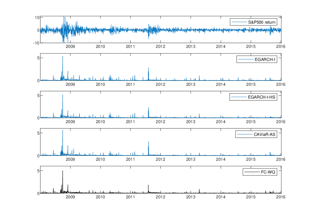
In addition, for S&P 500 the quantile loss values for each time step across the whole forecasting period are visualised in Figure 1. Namely, EGARCH-t, EGARCH-t-HS, CAViaR-AS (used in the WQ approach of Storti and Wang 2021) and FC-WQ are compared. The forecast combination is evidently characterized by more “stabilized” quantile loss values. For example, between 2009 and 2012, the quantile loss from the forecast combination approach is consistently smaller than that of the competing models, including the EGARCH-t-HS and CAViaR-AS which have good quantile loss performance as shown in Table 2. Therefore, the proposed forecast combination not only allows obtaining an improved predictor via combining different functional forms, i.e., parametric and semi-parametric models, but also produces more robust and stabilized quantile forecasts through the quantile combination process. Such time stability argument is consistent with the aim of forecast combinations that is to account for model uncertainty and to provide a forecasting performance that is optimal (or close to being optimal) and stable across time, which is supported by the results in Table 1, 2 and Figure 1.
Lastly, to further assess the validity of the quantile forecast combination, we have employed the VaR calibration tests defined in Patton et al. 2019, with the code developed by the authors. The test employs a MZ type regression of generalized VaR residuals on fitted VaR and lagged generalized residuals. Regression coefficients are fitted by Ordinary Least Squares (OLS) and standard errors are computed by a Newey-West estimator with 20 lags. The p-values of each data set and model produced from the test are presented in Table 3. In addition, on the 10% significance level, the column “Total” shows the total number of rejections (p-value less than 10%) for each model. Regarding the results, CAViaR-AS receives the least number of rejections and is closely followed by several models, including the proposed FC-WQ, which are rejected twice. The GJR-GARCH-t and EGARCH-t models are the most frequently rejected by the test.
| Model | S&P500 | HangSeng | FTSE | DAX | SMI | ASX200 | Total |
|---|---|---|---|---|---|---|---|
| GJR-GARCH-t | 0.003 | 0.494 | 0.010 | 0.001 | 0.025 | 0.002 | 5 |
| EGARCH-t | 0.056 | 0.576 | 0.018 | 0.006 | 0.002 | 0.024 | 5 |
| POT-GJR-GARCH-t | 0.255 | 0.948 | 0.750 | 0.037 | 0.000 | 0.000 | 3 |
| POT-EGARCH-t | 0.740 | 0.936 | 0.757 | 0.639 | 0.059 | 0.000 | 2 |
| GJR-GARCH-t-HS | 0.255 | 0.953 | 0.807 | 0.037 | 0.000 | 0.000 | 3 |
| EGARCH-t-HS | 0.740 | 0.936 | 0.838 | 0.706 | 0.074 | 0.000 | 2 |
| CAViaR-AS | 0.816 | 0.849 | 0.796 | 0.501 | 0.106 | 0.000 | 1 |
| CARE-AS | 0.910 | 0.610 | 0.734 | 0.605 | 0.097 | 0.000 | 2 |
| FC-WQ | 0.932 | 0.682 | 0.873 | 0.738 | 0.069 | 0.000 | 2 |
Note: Box indicates the favoured model and dashed box indicates the 2nd ranked model based on the total number of rejections on the 10% significance level. p-values are presented for each index and each model.
5.3 ES forecasts evaluation
We remind that a key feature of the proposed framework is that, for each trial quantile level, the combined VaR predictor can potentially have a different structure in terms of included models and assigned weights. This flexibility can only expected to be beneficial for the ES forecasting performance. Also, no specific assumptions are formulated on relationship linking VaR and ES but, consistently with its theoretical definition, ES is computed as a weighted average of combined VaR forecasts. This design naturally yields a combined ES predictor that has been purged of the impact of model uncertainty. Due to these features, it is expected that, compared to single forecasting models, the FC-WQ framework could be characterized by an improved and more stable ES forecasting performance. Aim of this section is to provide empirical evidence supporting this hypothesis.
In the FC-WQ framework, we consider and quantile trial levels for the weighted quantile process, with the corresponding framework named as FC-WQ-, . Storti and Wang 2021 show that the weighted quantile framework is not sensitive to the choice of , meaning a small value of , i.e., 3 or 5, can be chosen in real data applications to reduce the computation requirement.
The WQ approach employing CAViaR-AS for quantile estimation is also included for comparison. We name this model as CAViaR-AS-WQ. Again, and quantile trial levels are considered for the CAViaR-AS-WQ model (CAViaR-AS-WQ-3, CAViaR-AS-WQ-5).
In addition, we also test the ES forecasting performance via incorporating the Simple Average of the combined quantile forecasts (FC-SA), as in below Equation (24). The value of is also selected as 3 and 5 respectively.
| (24) |
Lastly, the Simple Average of the CAViaR-AS estimated quantiles (CAViaR-AS-SA) is included, with the value of chosen as 3 and 5 respectively as well.
To evaluate the FC-WQ framework comprehensively, we assess the ability of the different models under comparison to forecast VaR and ES jointly, employing the joint loss values in Equation (6). We use this to jointly compare the VaR and ES forecasts from all models, because the AL log-score in Equation (6) is a strictly consistent scoring function that is jointly minimized by the true VaR and ES series.
First, Figure 2 shows the S&P500 ES forecasts from EGARCH-t, EGARCH-t-HS, ES-CAViaR-Mult-AS, CAViaR-AS-WQ-3 and FC-WQ-3. To make a more in-depth comparison of these models, Figure 3 presents the S&P 500 AL joint loss (log-score) values for each time step across the out-of-sample period. In general, we have a consistent story as in the quantile loss plot in Figure 1. The ES forecasts produced from FC-WQ framework are again characterized by more stabilized and smaller joint loss values (i.e., the 2009 to 2012 period) than the ones from the competing individual and CAViaR-AS-WQ models, such as EGARCH-t, EGARCH-t-HS, ES-CAViaR-Mult-AS and CAViaR-AS-WQ-3.


Table 4 reports, for each model and data series, the value of the loss function in Equation (6) aggregated over the out-of-sample period: , with . In general, the proposed FC-WQ models produce on average the smallest joint loss, i.e, 4257.6 for FC-WQ-3 and 4257.8 for FC-WQ-5. The results of FC-WQ-3 and FC-WQ-5 are quite close to each other, which is consistent with the observations in Storti and Wang 2021 and means the choice of can already produce ES forecast with good accuracy.
Comparing the FC-WQ and CAViaR-AS-WQ results, the FC-WQ produces smaller joint loss values, which lends evidence on the improved quantile and ES forecasts via the proposed quantile forecast combination and weighed quantile approach. The effectiveness of quantile forecast combination is also supported by the findings that the FC-SA models produce smaller joint loss values than the CAViaR-AS-SA models.
The FC-SA framework produces joint loss values which are consistently larger than that from the corresponding FC-WQ, i.e., comparing FC-SA-M to FC-WQ-M (). Similar findings are observed when comparing CAViaR-AS-SA and CAViaR-AS-WQ. This lends evidence on the effectiveness of employing the Beta weighting scheme on the combined quantile forecasts. Lastly, GJR-GARCH-t and EGARCH-t, which are included in the model universe of the FC-WQ framework, are least preferred, with average loss as 4314.8 and 4315.1 respectively.
| Model | S&P500 | HangSeng | FTSE | DAX | SMI | ASX200 | Avg Loss |
|---|---|---|---|---|---|---|---|
| GJR-GARCH-t | 4239.2 | 4601.7 | 4183.8 | 4601.4 | 4253.6 | 4009.1 | 4314.8 |
| EGARCH-t | 4290.6 | 4586.9 | 4192.1 | 4585.2 | 4245.2 | 3990.4 | 4315.1 |
| POT-GJR-GARCH-t | 4175.3 | 4587.6 | 4131.4 | 4557.7 | 4215.5 | 3963.5 | 4271.8 |
| POT-EGARCH-t | 4226.2 | 4575.6 | 4146.7 | 4543.2 | 4185.6 | 3954.6 | 4272.0 |
| GJR-GARCH-t-HS | 4174.1 | 4587.7 | 4131.3 | 4556.6 | 4216.0 | 3962.5 | 4271.3 |
| EGARCH-t-HS | 4225.1 | 4575.0 | 4146.9 | 4542.8 | 4185.5 | 3953.9 | 4271.5 |
| CARE-AS | 4276.8 | 4550.7 | 4160.6 | 4514.8 | 4252.5 | 4024.9 | 4296.7 |
| ES-CAViaR-Add-AS | 4242.3 | 4551.9 | 4131.8 | 4506.8 | 4192.1 | 3992.9 | 4269.6 |
| ES-CAViaR-Mult-AS | 4242.3 | 4564.2 | 4117.8 | 4509.1 | 4188.3 | 3977.4 | 4266.5 |
| CAViaR-AS-SA-3 | 4265.5 | 4550.9 | 4145.5 | 4519.2 | 4214.4 | 3988.1 | 4280.6 |
| CAViaR-AS-SA-5 | 4275.3 | 4553.0 | 4147.5 | 4525.4 | 4218.2 | 3984.9 | 4284.0 |
| CAViaR-AS-WQ-3 | 4252.6 | 4549.4 | 4130.4 | 4507.7 | 4195.2 | 3982.4 | 4269.6 |
| CAViaR-AS-WQ-5 | 4255.0 | 4550.9 | 4135.6 | 4513.3 | 4195.2 | 3979.4 | 4271.6 |
| FC-SA-3 | 4157.7 | 4572.8 | 4138.7 | 4551.7 | 4211.5 | 3966.8 | 4266.5 |
| FC-SA-5 | 4149.7 | 4568.1 | 4182.3 | 4534.7 | 4213.1 | 3946.6 | 4265.8 |
| FC-WQ-3 | 4152.9 | 4568.1 | 4136.5 | 4537.1 | 4193.7 | 3957.5 | 4257.6 |
| FC-WQ-5 | 4141.9 | 4565.6 | 4174.6 | 4520.8 | 4198.6 | 3945.6 | 4257.8 |
Note:Box indicates the favoured model and dashed box indicates the 2nd ranked model based on the average loss.
Lastly, similar to the VaR calibration test, following Patton et al. 2019 an ES regression-based calibration test is also conducted with results shown in Table 5. Overall, the observations are similar to that of the VaR calibration test. On the 10% significance level, the proposed FC-WQ framework together with FC-SA and CARE-AS are least likely to be rejected by the test, compared with other competing models. The CAViaR-AS-WQ and CAViaR-AS-SA models are rejected on 3 markets via the calibration test. The GJR-GARCH-t and EGARCH-t are rejected for all six data sets. However, the proposed FC-WQ framework which includes the GJR-GARCH-t and EGARCH-t in its model universe can still produce competitive ES forecasts via the quantile forecast combination and weighting scheme, which again lends support on its effectiveness.
| Model | S&P500 | HangSeng | FTSE | DAX | SMI | ASX200 | Total |
|---|---|---|---|---|---|---|---|
| GJR-GARCH-t | 0.000 | 0.037 | 0.000 | 0.000 | 0.000 | 0.000 | 6 |
| EGARCH-t | 0.003 | 0.066 | 0.000 | 0.000 | 0.000 | 0.001 | 6 |
| POT-GJR-GARCH-t | 0.067 | 0.368 | 0.135 | 0.003 | 0.000 | 0.000 | 4 |
| POT-EGARCH-t | 0.201 | 0.338 | 0.161 | 0.079 | 0.008 | 0.000 | 3 |
| GJR-GARCH-t-HS | 0.069 | 0.420 | 0.175 | 0.003 | 0.000 | 0.000 | 4 |
| EGARCH-t-HS | 0.205 | 0.345 | 0.207 | 0.091 | 0.011 | 0.000 | 3 |
| CARE-AS | 0.508 | 0.473 | 0.122 | 0.180 | 0.009 | 0.000 | 2 |
| ES-CAViaR-Add-AS | 0.241 | 0.725 | 0.123 | 0.059 | 0.014 | 0.000 | 3 |
| ES-CAViaR-Mult-AS | 0.298 | 0.696 | 0.086 | 0.055 | 0.018 | 0.000 | 4 |
| CAViaR-AS-SA-3 | 0.285 | 0.695 | 0.169 | 0.059 | 0.013 | 0.000 | 3 |
| CAViaR-AS-SA-5 | 0.292 | 0.670 | 0.173 | 0.058 | 0.013 | 0.000 | 3 |
| CAViaR-AS-WQ-3 | 0.291 | 0.612 | 0.137 | 0.061 | 0.012 | 0.000 | 3 |
| CAViaR-AS-WQ-5 | 0.296 | 0.579 | 0.139 | 0.060 | 0.012 | 0.000 | 3 |
| FC-SA-3 | 0.458 | 0.541 | 0.311 | 0.131 | 0.007 | 0.000 | 2 |
| FC-SA-5 | 0.729 | 0.506 | 0.343 | 0.170 | 0.004 | 0.000 | 2 |
| FC-WQ-3 | 0.459 | 0.553 | 0.306 | 0.119 | 0.009 | 0.000 | 2 |
| FC-WQ-5 | 0.712 | 0.450 | 0.344 | 0.166 | 0.006 | 0.000 | 2 |
Note: Box indicates the favoured model and dashed box indicates the 2nd ranked model based on the total number of rejections on the 10% significance level. p-values are presented for each index and each model.
6 Conclusion
In this paper, in order to reduce the impact of model uncertainty in tail risk forecasting, we propose an innovative framework based on a forecast combination and weighted quantile (FC-WQ) approach that extends the WQ approach in Storti and Wang 2021. The first step forecast combination procedure combines quantile forecasts from all VaR models included in the model universe, on a grid of quantile levels. Then, the combined quantiles forecasts are employed as input to a quantile weighting scheme which is used to produce ES forecasts. The coefficients involved in the two steps of the procedure are estimated via optimizing the quantile loss and a strictly consistent joint VaR and ES loss, respectively. The selected model universe consists of parametric and semi-parametric models.
Compared to the VaR & ES forecast combination approach in Taylor 2020, which combines “pairs” of VaR & ES forecasting from various models, our approach breaks the tie between the VaR and ES model, and only requires VaR forecasts from individual VaR models. Therefore, we implicitly consider a greater variety of functional forms without making the number of parameters explode.
In a comprehensive empirical study, improvements in the out-of-sample forecasting of tail risks, especially ES, are observed, compared to each individual model in the model universe, the simple average approach and the WQ approach of Storti and Wang 2021. A further advantage of the proposed forecast combination and weighted quantile framework is its attitude to return “stabilized” quantile and joint loss values.
The proposed framework can be extended in a number of directions. First, other quantile forecast combination schemes, i.e., considering a multivariate quantile framework in the spirit of White et al. 2010, could be considered as alternatives. Second, the first step quantile forecast combination approach could be replaced by a cross validation approach which selects one model for each quantile level in the chosen grid. Third, a greater range of models, such as the ones incorporating high frequency based realized measures, could be included in the model universe. All these extensions are currently left for future investigation.
References
- Acerbi and Tasche (2002) Acerbi, C. and D. Tasche (2002). Expected shortfall: A natural coherent alternative to value at risk. Economic Notes 31(2), 379–388.
- Aigner et al. (1976) Aigner, D. J., T. Amemiya, and D. J. Poirier (1976). On the estimation of production frontiers: Maximum likelihood estimation of the parameters of a discontinuous density function. International Economic Review 17(2), 377–396.
- Artzner (1997) Artzner, P. (1997). Thinking coherently. Risk, 68–71.
- Artzner et al. (1999) Artzner, P., F. Delbaen, J. Eber, and D. Heath (1999). Coherent measures of risk. Mathematical Finance 9(3), 203–228.
- Basel Committee on Banking Supervision (2019) Basel Committee on Banking Supervision (2019). Minimum capital requirements for market risk. Bank for International Settlements.
- Bollerslev (1986) Bollerslev, T. (1986). Generalized autoregressive conditional heteroskedasticity. Journal of econometrics 31(3), 307–327.
- Chernozhukov et al. (2010) Chernozhukov, V., I. Fernández-Val, and A. Galichon (2010). Quantile and probability curves without crossing. Econometrica 78(3), 1093–1125.
- Creal et al. (2013) Creal, D., S. J. Koopman, and A. Lucas (2013). Generalized autoregressive score models with applications. Journal of Applied Econometrics 28(5), 777–795.
- Engle and Manganelli (2004) Engle, R. F. and S. Manganelli (2004). Caviar: Conditional autoregressive value at risk by regression quantiles. Journal of Business & Economic Statistics 22(4), 367–381.
- Fissler and Ziegel (2016) Fissler, T. and J. F. Ziegel (2016). Higher order elicitability and Osband’s principle. The Annals of Statistics 44(4), 1680–1707.
- Giacomini and Komunjer (2005) Giacomini, R. and I. Komunjer (2005). Evaluation and combination of conditional quantile forecasts. Journal of Business & Economic Statistics 23(4), 416–431.
- Gilli et al. (2006) Gilli, M. et al. (2006). An application of extreme value theory for measuring financial risk. Computational Economics 27(2), 207–228.
- Glosten et al. (1993) Glosten, L. R., R. Jagannathan, and D. E. Runkle (1993). On the relation between the expected value and the volatility of the nominal excess return on stocks. The journal of finance 48(5), 1779–1801.
- Harvey (2013) Harvey, A. (2013). Dynamic Models for Volatility and Heavy Tails. Econometric Society Monographs.
- Koenker and Machado (1999) Koenker, R. and J. A. F. Machado (1999). Goodness of fit and related inference processes for quantile regression. Journal of the American Statistical Association 94(448), 1296–1310.
- McNeil and Frey (2000) McNeil, A. J. and R. Frey (2000). Estimation of tail-related risk measures for heteroscedastic financial time series: an extreme value approach. Journal of empirical finance 7(3-4), 271–300.
- Nelson (1991) Nelson, D. B. (1991). Conditional heteroskedasticity in asset returns: A new approach. Econometrica: Journal of the Econometric Society, 347–370.
- Newey and Powell (1987) Newey, W. K. and J. L. Powell (1987). Asymmetric least squares estimation and testing. Econometrica 55(4), 819–847.
- Patton et al. (2019) Patton, A. J., J. F. Ziegel, and R. Chen (2019). Dynamic semiparametric models for expected shortfall (and value-at-risk). Journal of Econometrics 211(2), 388 – 413.
- Storti and Wang (2021) Storti, G. and C. Wang (2021). Nonparametric expected shortfall forecasting incorporating weighted quantiles. International Journal of Forecasting. In press.
- Taylor (2008) Taylor, J. W. (2008). Estimating value at risk and expected shortfall using expectiles. Journal of Financial Econometrics 6(2), 231–252.
- Taylor (2019) Taylor, J. W. (2019). Forecasting value at risk and expected shortfall using a semiparametric approach based on the asymmetric laplace distribution. Journal of Business & Economic Statistics 37(1), 121–133.
- Taylor (2020) Taylor, J. W. (2020). Forecast combinations for value at risk and expected shortfall. International Journal of Forecasting 36(2), 428–441.
- White et al. (2010) White, H., T.-H. Kim, and S. Manganelli (2010). Modeling Autoregressive Conditional Skewness and Kurtosis with Multi-Quantile CAViaR. United Kingdom: Oxford University Press.