Optimal design versus maximal Monge-Kantorovich metrics

Karol Bołbotowski and Guy Bouchitté

Date: August 11, 2026

Abstract.

A remarkable connection between optimal design and Monge transport was initiated in the years 1997 in the context of the minimal elastic compliance problem and where the euclidean metric cost was naturally involved. In this paper we present different variants in optimal design of mechanical structures, in particular focusing on the optimal pre-stressed elastic membrane problem. We show that the underlying metric cost is associated with an unknown maximal monotone map which maximizes the Monge-Kantorovich distance between two measures. In parallel with the classical duality theory leading to existence and (in a smooth case) to PDE optimality conditions, we present a general geometrical approach arising from a two-point scheme in which geodesics with respect to the optimal metric play a central role. These two aspects are enlightened by several explicit examples and also by numerical solutions in which optimal structures very often turn out to be truss-like i.e supported by piecewise affine geodesics. In case of a discrete load, we are able to relate the existence of such truss-like solutions to an extension property of maximal monotone maps which is of independent interest and that we propose here as a conjecture.

Keywords: Minimal compliance, pres-stressed membrane, monotone maps, peusdo-metric, Monge-Kantorovich distance, geodesics, duality and saddle point

2010 Mathematics Subject Classification: 49J45, 49K20, 49J20, 90B06, 28A50, 74P05

1. introduction

The analysis of the behaviour of elastic structures has always been a central problem in Mathematics and in Engineering. In the last decades, the optimal design of such structures took benefit of the dramatic improvement of the powerful tools of calculus of variations and geometric measure theory which have been developed meanwhile. Among them homogenization and $\Gamma$ -convergence techniques allowed decisive breakdowns as for instance the emergence of topological optimization methods [2] which are now very popular in civil and mechanical engineering.

For the first time, in the year 1997, a remarkable connection between optimal design and Monge transport problem was discovered. It concerned specifically the classical optimal compliance problem in the scalar case [12] that may be related to designing a heat conductor and then it was developped further in the framework of elasticity [8]. This new approach turned out to be very fruitful as it was possible to consider concentrated loads $f$ and low dimensional structures as competitors, in particular trusses of bars as they appear in Michell problem [15] in case of a vanishing volume fraction limit of available elastic material. From the Monge-Kantorovich optimal transport point of view, the main limitation of this approach is that the underlying cost is always related to the Euclidean metric on the ambient space $\mathbb{R}^{d}$ ( $d=2$ or $d=3$ in practice).

In this work we will bring to the fore a new family of optimal design problems for which the Monge-Kantorovich approach mentioned above can be used but needs to be adapted with a major modification: the transport cost is now an unknown that will be determined by solving a maximization problem in a suitable class of admissible metric costs on $\mathbb{R}^{d}$ (including the Euclidean one). This family includes the two-dimensional problem of designing a membrane subject to an out-of-plane load $f$ . Two approaches can be distinguished:

(A) The optimal elastic membrane problem which relies on a non-linear model inspired by the von Kármán’s plate theory (see e.g. [21], Section 6 in [28], Section II.4 in [31]); the design variable is a mass distribution $\mu$ for which the in-plane stress field $\sigma$ is an effect of elastic response to the loads;

(B) The simplified optimal pre-stressed membrane problem which relies on the classical linear model (see e.g. Section IV.10.3 in [23]) where the design variable is the (non-negative) in-plane stress field $\sigma$ which is subject to the equilibrium constraint.

Note that in both cases the transverse stiffness of the membrane does not depend directly on the constitutive law of the underlying elastic material but of the in-plane stress field $\sigma$ which point-wisely is a positive semi-definite symmetric tensor. It turns out that the two problems above are in some sense equivalent to each other and surprisingly also to another 3D design problem that fits into a class of long standing engineering problems of form finding:

(C) The optimal vault problem where over a horizontal 2D reference domain one is to find a surface $z=z(x_{1},x_{2})$ and elastic material’s distribution on this surface. The shell/vault thus constructed ought to carry the vertical load $f$ by means of compression only; vertical position of the load is a design variable, i.e. $f$ tracks the shape $z$ of the vault.

The equivalence between (C) and (B) is established in a recent work of the first author [5] where (C) appears as a generalization of the Rozvany-Prager optimal arch-grid problem [33], [24] (the latter one being recovered when the vault must compose of two mutually orthogonal families of arches).

A detailed presentation of the different optimal design problems sketched above will be skipped for the sake of conciseness but we ask to keep in mind that they all lead precisely to the same mathematical framework, up to changing the mechanical interpretation of the paramaters coming into play. In the present paper we will focus on model (B) namely the optimal pre-stressed membrane problem. The motivation for choosing this variant is that it can be obtained through a simple modification of the classical optimal compliance model in the spirit of [8, 12] and then we may describe step by step how we pass from the Monge OT approach involving the Euclidean cost to a model requiring the identification of an optimal metric cost.

In a first step let us briefly describe the scalar mass optimization and its variant we call free material design problem (see [6] for the vectorial variant). Given a bounded domain $\Omega\subset\mathbb{R}^{d}$ (design region), $\Sigma_{0}$ being a compact subset of ${\overline{\Omega}}$ and a bounded signed Radon measure $f\in{\mathcal{M}}({\overline{\Omega}};\mathbb{R})$ , we consider an unknown mass distribution $\mu\in{\mathcal{M}}_{+}({\overline{\Omega}})$ of material and define the compliance to be

\mathcal{E}_{\Omega,f,\Sigma_{0}}(\mu)=\mathcal{E}(\mu)=\sup\left\{\int u\,df-\frac{1}{2}\int{\left\lvert\nabla u\right\rvert}^{2}d\mu\ :\ u\in\mathcal{D}(\mathbb{R}^{d})\ ,\ u=0\ \text{on $\Sigma_{0}$}\right\}.

The mass optimization problem (MOP) with respect to a given amount of mass $m$ reads as follows

MOP)\beta(m):=\inf\left\{{\mathcal{C}}(\mu):\mu\in{\mathcal{M}}_{+}({\overline{\Omega}}),\,\int d\mu\leq m\right\}

(()

If $\Sigma_{0}$ is void (pure Neumann problem) we need to assume that $f$ is balanced, i.e. $\int f^{+}=\int f^{-}$ . Then if $\Omega$ is convex it is shown in [8] that $\displaystyle\beta(m)=\frac{(W_{1}(f^{+},f^{-}))^{2}}{2m}\ ,$ where

W_{1}(f^{+},f^{-})=\inf\left\{\int_{{\overline{\Omega}}\times{\overline{\Omega}}}|x-y|\,\gamma(dxdy)\,:\,\gamma\in\Gamma(f^{+},f^{-})\right\}

(1.1)

denotes the Monge-Kantorovich distance and $\gamma\in\Gamma(f^{+},f^{-})$ means that $\gamma$ as a measure on ${\mathcal{M}}_{+}\bigl({\overline{\Omega}}^{2}\bigr)$ (transport plan) admits $f^{+},f^{-}$ as marginals. Notice that, if $\Omega$ is non-convex, we simply need to substitute $|x-y|$ with the geodesic distance in $\Omega$ between $x$ and $y$ . In case $\Sigma_{0}$ is a non-empty compact subset of $\partial\Omega$ and $f$ is a non-negative measure (that is $f^{-}=0$ ), the latter formula for the infimum of $\mathrm{(MOP)}$ can be recast from the Monge distance of $f$ to $\Sigma_{0}$ namely (see [12])

\beta(m):=\inf(\mathrm{MOP})=\frac{\bigl(W_{1}(f,\Sigma_{0})\bigr)^{2}}{2m},

(1.2)

where

W_{1}(f,\Sigma_{0}):=\min\Big\{W_{1}(f,\nu)\,:\,\nu\in{\mathcal{M}}_{+}(\Sigma_{0})\Big\}=\int\mathrm{dist}(x,\Sigma_{0})\,f(dx).

(1.3)

Then a geometric characterization of optimal $\mu$ can be deduced from the geodesics transport rays connecting points in the support of $f$ to $\Sigma_{0}$ . Let us mention that the case where $\Sigma_{0}=\partial\Omega$ is classical in sandpile models (see for instance [18]).

Next, an anisotropic generalization of the $\mathrm{(MOP)}$ problem can be considered in which, instead of looking at optimal mass distributions, we search for optimal conductivity tensor field $\sigma\in{\mathcal{M}}({\overline{\Omega}};{\mathcal{S}^{d\times d}_{+}})$ where ${\mathcal{S}^{d\times d}_{+}}$ is the set of positive semi-definite symmetric tensors:

FMD)\inf\biggl\{{\mathcal{C}}(\sigma)\,:\,\sigma\in{\mathcal{M}}({\overline{\Omega}};{\mathcal{S}^{d\times d}_{+}}),\ \frac{1}{d}\int{\mathrm{Tr}}\,\sigma\leq m\biggr\}

(()

where, for a prescribed Dirichlet region $\Sigma_{0}$ , the compliance reads

{\mathcal{C}}(\sigma)=\sup\left\{\int u\,df-\frac{1}{2}\int{\left\langle\sigma,\nabla u\otimes\nabla u\right\rangle}\ :\ u\in\mathcal{D}(\mathbb{R}^{d}),\ u=0\ \text{on $\Sigma_{0}$}\right\}.

(1.4)

With the notations above, we see that for $\sigma={\mathrm{Id}}\,\mu$ it holds ${\mathcal{C}}(\sigma)=\mathcal{E}(\mu)$ and the choice of the constraint to be the integral of the trace of $\sigma$ , although debatable, intends to be the natural counterpart of the mass constraint in (MOP). Note that in the vector case of linear elasticity, the design variable $\sigma$ is rather a fourth order tensor (inducing Hooke’s law) and the related version of (FMD) is more involved (see the recent work [6]). Nevertheless, as will be seen later, the (FMD) variant is very close fo the initial (MOP) problem and optimal solutions $\sigma$ can be recovered in the same way by selecting geodesics with respect to the Euclidean metric.

We may now readily pass to the optimal pre-stressed membrane model. As in the (FMD) problem, the unknown design variable is an element of ${\mathcal{M}}({\overline{\Omega}};{\mathcal{S}^{d\times d}_{+}})$ whereas now the tensor measure $\sigma$ represents the in-plane stress in the membrane occupying a plane horizontal domain $\Omega$ . The positivity condition imposed on $\sigma$ rules out compressive stress, which is reasonable when the membrane is very thin and thus perfectly immune to buckling. We assume that the membrane is subject to vertical pressure $f\in{\mathcal{M}}({\overline{\Omega}};\mathbb{R})$ and to an in-plane load exerted on the boundary only. The latter forces depend on the designer and play the role of a pre-load that generates the pre-stress $\sigma$ in the whole domain which in turn provides stiffness against $f$ . Since in the interior of the design region only the out-of-plane component of load is non-zero the in-plane equilibrium requires that ${\mathrm{Div}}\,{\sigma}=0$ in the distributional sense in $\Omega$ . Virtually, it is the divergence free condition on $\sigma$ that converts the (FMD) problem for heat conductor to the optimal design model for a pre-stressed membrane:

OM)\inf\biggl\{{\mathcal{C}}(\sigma)\,:\,\sigma\in{\mathcal{M}}({\overline{\Omega}};{\mathcal{S}^{d\times d}_{+}}),\,{\mathrm{Div}}\sigma=0\ \text{in $\Omega$},\ \frac{1}{d}\int{\mathrm{Tr}}\,\sigma\leq m\biggr\},

(()

where the load $f$ enters through ${\mathcal{C}}(\sigma)$ (defined in (1.4)) together with $\Sigma_{0}$ being the part of the boundary where the membrane is pinned in the vertical direction; the function $u$ represents deflection (the out-of-plane displacement) of the membrane.

A first observation is that the problems (FMD) and (OM) do not share the same infimum in general. This is due to the divergence constraint which rules out many possible competitors. In particular:

•

An isotropic tensor field of the kind $\sigma=a(x)\,{\mathrm{Id}}\ \mathcal{L}^{2}\mathbin{\vrule height=6.88889pt,depth=0.0pt,width=0.55974pt\vrule height=0.55974pt,depth=0.0pt,width=5.59721pt}\Omega$ is not admissible unless $a$ is constant.
•

Let $\sigma=p(x)\,\tau(x)\otimes\tau(x)\,\mathcal{H}^{1}\mathbin{\vrule height=6.88889pt,depth=0.0pt,width=0.55974pt\vrule height=0.55974pt,depth=0.0pt,width=5.59721pt}C$ with $C$ being a simple curve, $p(x)$ a positive weight and $\tau(x)$ a unit vector vector. Then $\sigma$ is admissible iff $C$ is a straight line connecting two points of $\partial\Omega$ while $\tau$ is a constant vector parallel to $C$ and $p$ is constant.

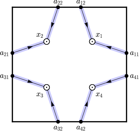
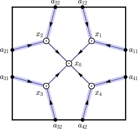
In fact as will be seen later, pre-stress tensor fields supported by networks of bars or, as they should be called within the membrane model, strings are favoured in the (OM) problem. To give a flavour of the geometry of solutions, we illustrate in Figure 1 below the optimal configurations for (FMD) and (OM) in the case where $f$ is a single Dirac pressure exerted at a point of a square membrane which is pinned along all its boundary, i.e. $\Sigma_{0}=\partial\Omega$ . For (OM) problem the support of optimal measure $\sigma$ is described by a finite union of strings of different thickness that are tied at the loaded point. Such lower dimensional solutions shall be referred to as trusses or truss structures. In Figure 1 the arrows indicate the direction of the gradient flow of the deflection function $u$ .

An unexpected discovery we wish to promote in this paper is that the (OM) problem has a very deep relation with another interesting issue in geometry and optimal transport theory: the search of optimal metrics in a suitable class which maximize the associated Monge distance between two measures. More precisely, if we consider the membrane problem for $\Sigma_{0}=\partial\Omega$ and $f\in{\mathcal{M}}_{+}(\Omega)$ , then it holds that $\min(\mathrm{OM})=\frac{Z_{0}^{2}}{2m_{0}}$ where $Z_{0}=Z_{0}(f,\Omega)$ is given by

Z_{0}=\sup\Big\{W_{c_{v}}(f,\partial\Omega)\ :\ v\in C^{\infty}(\mathbb{R}^{2};\mathbb{R}^{2}),\ e(v)\geq 0,\ v={\mathrm{id}}\ \text{in $\mathbb{R}^{2}\setminus{\overline{\Omega}}$}\Big\},

(1.5)

where $e(v)$ is the symmetrized gradient of $v$ , $c_{v}$ is the geodesic distance associated with the metric tensor $e(v)$ and $W_{c_{v}}$ stands for the Monge distance related to the cost $c_{v}$ . Our results include the existence of an optimal maximal monotone map $v$ for a relaxed version of the right hand member of (1.5). Note that the problem of maximizing a geodesic distance among particular classes of scalar metrics has been considered in a different context by several authors [29], [36].

The paper is organized as follows:

In Section 2, we revisit the link between the (FMD) problem and Monge-Kantorovich theory in the spirit of [8]. In particular we establish an equivalence between (MOP) and (FMD) and we give a full description of the optimal measure $\sigma$ in terms of the transport rays connecting the support of $f$ to the boundary of $\partial\Omega$ . In addition we show that the strict inequality $\inf\mathrm{(FMD)}<\inf\mathrm{(OM)}$ holds unless the load $f$ is supported on a geometrically identifiable compact subset of $\Omega$ .

In Section 3, we show the existence of an optimal $\sigma\in{\mathcal{M}}({\overline{\Omega}};{\mathcal{S}^{d\times d}_{+}})$ for (OM) and we develop a primal-dual framework based on the introduction of an additional unknown horizontal vector field $w:\Omega\to\mathbb{R}^{2}$ vanishing on $\partial\Omega$ whose symmetrized distributional gradient will play the role of a Lagrange multiplier for the divergence free constraint. Accordingly we are led to a dual problem

Z_{0}:=\sup\left\{{\left\langle f,u\right\rangle}\ :\ e(w)+\frac{1}{2}\,\nabla u\otimes\nabla u\leq{\mathrm{Id}}\right\}

(1.6)

where pairs $(u,w)$ are in duality with measures $(\lambda,\sigma)\in{\mathcal{M}}({\overline{\Omega}};\mathbb{R}^{d})\times{\mathcal{M}}({\overline{\Omega}};{\mathcal{S}^{d\times d}})$ ( $\lambda$ coresponds to the transverse internal force in the membrane caused by its deflection). Then, upon rewriting the constraint in (1.6) in terms of an equivalent two points conditions, namely:

\frac{1}{2}\,|u(y)-u(x)|^{2}+{\left\langle w(y)-w(x),y-x\right\rangle}\leq|x-y|^{2}\hskip 20.00003pt\forall(x,y)\in({\overline{\Omega}})^{2},

(1.7)

we put forward an alternative duality scheme which fits perfectly to characterize truss-like optimal pairs $(\lambda,\sigma)$ in the sense that they are decomposable in the form $(\lambda_{\pi},\sigma_{\Pi})$ given in (1.10), (1.11). Here, as far as they exist, $\pi$ and $\Pi$ are measures on ${\overline{\Omega}}\times{\overline{\Omega}}$ which play the role of Lagrange multipliers of the two-point constraint (1.7).

In Section 4, we give necessary and sufficient conditions of optimality for two pairs $(\lambda,\sigma)$ and $(u,w)$ assuming that $(u,w)$ is Lipschitz regular. These conditions are particularized in the case of a truss configuration $(\lambda,\sigma)=(\lambda_{\pi},\sigma_{\Pi})$ . Then, examples of explicit optimal configurations are established in the radial case or for the load $f$ being a single Dirac mass (confirming in particular the optimality of the structure depicted in Figure 1(b)).

In Section 5, we exploit the two-point condition (1.7) to establish a connection between the optimal membrane problem $\mathrm{(OM)}$ and the search of a monotone map $v={\mathrm{id}}-w$ maximizing a Monge-Kantorovich distance as stated in (1.5). To that aim we begin with a preliminary subsection which could be considered of independent interest where we define the intrinsic pseudo-distance $c_{v}$ associated with a maximal monotone map $v:\mathbb{R}^{d}\to\mathbb{R}^{d}$ which agrees with the identity outside ${\overline{\Omega}}$ . Then we prove the existence of a maximal monotone $v$ associated with the worst Monge-Kantorovich metric (1.5) and derive a saddle point characterization of an optimal pair $(v,\gamma)$ where $\gamma$ is selected among the optimal transports plans solving $W_{c_{v}}(f,\partial\Omega)=\inf\bigl\{\int_{{\overline{\Omega}}\times{\overline{\Omega}}}c_{v}(x,y)\,\gamma(dxdy)\,:\,\gamma\in\Gamma(f,\nu),\ \nu\in{\mathcal{M}}_{+}(\partial\Omega)\bigr\}.$ Next we give a general criterium of optimality for a truss solution and establish the existence of such a solution in case of a finitely supported load $f$ assuming an extension property for monotone maps that we conjecture to be true.

In Section 6, we present several numerical simulations for the (OM) problem taking for design subset $\Omega$ a squared domain in $\mathbb{R}^{2}$ . It turns out that in most cases optimal stress measures $\sigma$ exhibit a truss structure. The numerical method is based on a duality scheme which involves the two-point condition (1.7) restricted to a discrete subset of ${\overline{\Omega}}\times{\overline{\Omega}}$ . It is worked out through a conic programming algorithm introduced recently in [5].

Eventually we provide in the appendix several classical tools of convex analysis, a short survey about tangential calculus with respect to a measure and some useful approximation properties of convex functions of measures.

To conclude this introduction, let us point out that the existence issue for the coupling measures $(\pi,\Pi)$ allowing the truss representation of a solution $(\lambda,\sigma)$ (see (1.10), (1.11)) is not ensured in general for the infinite dimensional setting. However we expect it to be true in the case of a finitely supported measure $f$ once the extension property for monotone metrics conjectured in Section 5 can be proved.

Acknowledgements

The first author is grateful to the Laboratoire IMATH, Université de Toulon for hosting his two-month visit there in the fall of 2019 where this research was initiated. He would also like to thank the National Science Centre (Poland) for the financial support and acknowledge the Research Grant no 2019/33/B/ST8/00325 entitled ”Merging the optimum design problems of structural topology and of the optimal choice of material characteristics. The theoretical foundations and numerical methods”.

Notations

Throughout the paper we will use the following notations:

-

$\Omega$ denotes a bounded domain of $\mathbb{R}^{d}$ that in general we assume to be convex; although our mechanical context requires $d=2$ , the mathematical arguments will often be valid for any natural $d$ ;
-

$\Sigma_{0}$ will be a compact subset of ${\partial\Omega}$ on which a Dirichlet condition is prescribed;
-

the Euclidean norm of $z\in\mathbb{R}^{d}$ is denoted by $|z|$ ; $S^{d-1}$ denores the unit sphere $\{|z|=1\}$ ;
-

by $\Delta$ we denote the diagonal of $\mathbb{R}^{d}$ , namely $\Delta=\bigl\{(x,x):x\in\mathbb{R}^{d}\bigr\}$ ;
-

by ${\mathcal{S}^{d\times d}}$ we shall see the space of $d\times d$ symmetric matrices, while ${\mathcal{S}^{d\times d}_{+}}$ will be its subset whose elements are positive semi-definite. Given $A,B\in{\mathcal{S}^{d\times d}}$ , we will write $A\leq B$ if $B-A\in{\mathcal{S}^{d\times d}_{+}}$ ; ${\mathrm{Tr}}A$ denotes the trace of $A$ , $\rk A$ the rank of $A$ ; ${\mathrm{Id}}$ denotes the identity matrix while ${\mathrm{id}}$ denotes the identity map on $\mathbb{R}^{d}$ ;
-

by $\mathbf{\chi}_{B}$ we will denote the indicator function of the set $B$ taking value $0$ in $B$ and $+\infty$ outside. Instead we denote by ${{\bf 1}\kern-2.79999pt\rm l}_{B}$ the characteristic function of $B$ taking value $1$ in $B$ and $0$ outside;
-

if $A\subset\mathbb{R}^{d}$ is an open subset, $\mathcal{D}(A)$ denotes be space of $C^{\infty}$ functions compactly supported in $A$ ; $\mathcal{D}({\overline{\Omega}}\setminus\Sigma_{0})$ denotes the set of restrictions to ${\overline{\Omega}}$ of elements in $\mathcal{D}(\mathbb{R}^{d}\setminus\Sigma_{0})$ ;
-

$C^{0}({\overline{\Omega}})$ denotes the Banach space of continuous functions on ${\overline{\Omega}}$ while $C_{\Sigma_{0}}({\overline{\Omega}})$ (resp. $C_{0}(\Omega)$ ) denotes the subset of $C^{0}({\overline{\Omega}})$ consisting of functions vanishing in $\Sigma_{0}$ (resp. in ${\partial\Omega}$ );
-

${\mathrm{Lip}}(\Omega)$ (or ${\mathrm{Lip}}({\overline{\Omega}})$ ) stands for the space of Lipschitz continuous functions on $\Omega$ (resp ${\overline{\Omega}}$ ) while ${\mathrm{Lip}}_{0}(\Omega)$ (resp. ${\mathrm{Lip}}_{\Sigma_{0}}(\Omega)$ ) denotes the subspace of elements vanishing on ${\partial\Omega}$ (resp. $\Sigma_{0}$ );
-

for $k>0$ , ${\mathrm{Lip}}_{k}(\Omega)$ is the subset of ${\mathrm{Lip}}(\Omega)$ of functions $u$ such that $|u(x)-u(y)|\leq k\;|x-y|$ for all $(x,y)$ (if $\Omega$ is convex, it coincides with $\{u\in W^{1,\infty}(\Omega):|\nabla u|\leq k\ \text{a.e.}\}$ );
-

${\mathcal{M}}_{+}(\mathbb{R}^{d})$ denotes the space of Borel measures on $\mathbb{R}^{d}$ with values in $[0,+\infty]$ . Unless explicitely specified, we will additionaly assume that elements of ${\mathcal{M}}_{+}(\mathbb{R}^{d})$ are finite on compact subsets; the topological support of $\mu\in{\mathcal{M}}_{+}(\mathbb{R}^{d})$ is denoted $\spt(\mu)$ while $\mu\mathop{\hbox{\vrule height=7.0pt,width=0.5pt,depth=0.0pt\vrule height=0.5pt,width=6.0pt,depth=0.0pt}}\nolimits A$ ; represents its trace on a Borel subset $A\subset\mathbb{R}^{d}$ ; ${\mathcal{M}}_{+}(A)$ will the subset of elements $\mu\in{\mathcal{M}}_{+}(\mathbb{R}^{d})$ such that $\mu=\mu\mathop{\hbox{\vrule height=7.0pt,width=0.5pt,depth=0.0pt\vrule height=0.5pt,width=6.0pt,depth=0.0pt}}\nolimits A$ (or such that $\spt(\mu)\subset A$ if $A$ is closed);
-

${\mathcal{M}}({\overline{\Omega}})$ (resp. ${\mathcal{M}}({\overline{\Omega}};\mathbb{R}^{d})$ or ${\mathcal{M}}({\overline{\Omega}};{\mathcal{S}^{d\times d}_{+}})$ ) is the space of signed finite Radon measures on $\mathbb{R}^{d}$ which are compactly supported in ${\overline{\Omega}}$ (resp. Borel regular measures from ${\overline{\Omega}}$ to $\mathbb{R}^{d}$ or ${\mathcal{S}^{d\times d}_{+}}$ ); given $\nu\in{\mathcal{M}}({\overline{\Omega}};\mathbb{R}^{d})$ and $\mu\in{\mathcal{M}}_{+}({\overline{\Omega}})$ , then $\nu\ll\mu$ means that $\nu=\zeta\mu$ for a suitable $\zeta\in L^{1}_{\mu}({\overline{\Omega}};\mathbb{R}^{d})$ whereas $\nu\perp\mu$ means that $\mu$ and $\nu$ are mutually singular;
-

for every Borel set $A$ , $\mathcal{P}(A):=\{\mu\in{\mathcal{M}}_{+}(A)\ :\ \mu(A)=1\}$ denotes the set of probalities on $A$ ;
-

given an open subset $A$ , $\mathcal{D}^{\prime}(A)$ denotes the set of distributions on $A$ (the dual of $\mathcal{D}(A)$ ); $\mathcal{D}^{\prime}({\overline{\Omega}})$ stands for the subset of $\mathcal{D}^{\prime}(\mathbb{R}^{d})$ consisting of distributions supported in ${\overline{\Omega}}$ ; to a distribution in $\mathcal{D}^{\prime}(\mathbb{R}^{d})$ we may associate its trace on any open subset $A$ defining a unique element of $\mathcal{D}^{\prime}(A)$ .
-

the distributional divergence of a matrix field $\sigma\in{\mathcal{M}}({\overline{\Omega}};{\mathcal{S}^{d\times d}_{+}})$ is an element in $\mathcal{D}^{\prime}(\mathbb{R}^{d};{\mathcal{S}^{d\times d}_{+}})$ that we will be denoted ${\mathrm{Div}}(\sigma)$ while ${\mathrm{div}}\lambda\in\mathcal{D}^{\prime}(\mathbb{R}^{d};\mathbb{R}^{d})$ will stand for the standard distributional divergence acting on a vector measure $\lambda\in{\mathcal{M}}({\overline{\Omega}};\mathbb{R}^{d})$ ; for $A$ being an open subset of $\mathbb{R}^{d}$ , the equality $-{\mathrm{div}}\lambda=f$ on $A$ means that the two distributions have the same trace on $A$ ;
-

the topological support of a function $f$ (resp.of a measure $\mu$ ) will be denoted $\spt(f)$ (resp. $\spt(\mu)$ );
-

the bracket ${\left\langle{\,\cdot\,},{\,\cdot\,}\right\rangle}$ shall be used to denote a canonical scalar product in the finite dimensional space of vectors or matrices, whilst in the case of infinite dimensional spaces we shall use the same bracket while sometimes specifying the functional spaces involved in the lower index;
-

$C^{0,\frac{1}{2}}({\overline{\Omega}})$ denotes the space of $\frac{1}{2}$ -Hölder continuous functions on $\Omega$ , while $C^{1}({\overline{\Omega}})$ denotes its subclass consisting of continuously differentiable functions;
-

given $\Sigma_{0}\subset{\partial\Omega}$ , for every $x\in{\overline{\Omega}}$ we denote by $d(\cdot,\Sigma_{0})$ the euclidean distance to $\Sigma_{0}$ and by $p_{\Sigma_{0}}(x)$ the subset of $\Sigma_{0}$ defined by

$p_{\Sigma_{0}}(x)=\Big\{z\in\Sigma_{0}\ :\ d(x,\Sigma_{0})=|x-z|\Big\};$ (1.8)

the graph of $p_{\Sigma_{0}}$ as a map from ${\overline{\Omega}}$ to subsets of $\Sigma_{0}$ will be denoted $G_{\Sigma_{0}}$ ;

for every $(x,y)\in{\overline{\Omega}}\times{\overline{\Omega}}$ such that $x\not=y$ , we denote by $\lambda^{x,y}$ and $\sigma^{x,y}$ the elements of ${\mathcal{M}}({\overline{\Omega}};\mathbb{R}^{d})$ and ${\mathcal{M}}({\overline{\Omega}};{\mathcal{S}^{d\times d}_{+}})$ , respectively, defined by:

\lambda^{x,y}=\tau^{x,y}\,\mathcal{H}^{1}\mathbin{\vrule height=6.88889pt,depth=0.0pt,width=0.55974pt\vrule height=0.55974pt,depth=0.0pt,width=5.59721pt}[x,y],\hskip 20.00003pt\sigma^{x,y}=\tau^{x,y}\otimes\tau^{x,y}\,\mathcal{H}^{1}\mathbin{\vrule height=6.88889pt,depth=0.0pt,width=0.55974pt\vrule height=0.55974pt,depth=0.0pt,width=5.59721pt}[x,y],\hskip 20.00003pt\tau^{x,y}=\frac{y-x}{|y-x|}

(1.9)

(by convention, we set $\lambda^{x,y}=0$ and $\sigma^{x,y}=0$ if $x=y$ ). Note that $\lambda^{y,x}=-\lambda^{x,y}$ while $\sigma^{y,x}=\sigma^{x,y}$ ;

for any $\pi\in{\mathcal{M}}({\overline{\Omega}}\times{\overline{\Omega}})$ , we denote by $\int\lambda^{x,y}\,\pi(dxdy)$ the measure $\lambda_{\pi}\in{\mathcal{M}}({\overline{\Omega}};\mathbb{R}^{d})$ such that

{\left\langle\lambda_{\pi},\psi\right\rangle}\ :=\ \int{\left\langle\lambda^{x,y},\psi\right\rangle}\,\pi(dxdy)\hskip 20.00003pt\forall\,\psi\in C^{0}({\overline{\Omega}},\mathbb{R}^{d});

(1.10)

for any $\Pi\in{\mathcal{M}}_{+}({\overline{\Omega}}\times{\overline{\Omega}})$ , we denote by $\int\sigma^{x,y}\,\Pi(dxdy)$ the measure $\sigma_{\Pi}\in{\mathcal{M}}({\overline{\Omega}};{\mathcal{S}^{d\times d}_{+}})$ such that

{\left\langle\sigma_{\Pi},\Psi\right\rangle}\ :=\ \int{\left\langle\sigma^{x,y},\Psi\right\rangle}\,\Pi(dxdy)\hskip 20.00003pt\forall\,\Psi\in C^{0}({\overline{\Omega}},{\mathcal{S}^{d\times d}_{+}}).

(1.11)

2. Monge-Kantorovich approach for the free material design problem

Throughout the whole section we will assume that the load $f$ is a non-negative measure that we normalize to satisfy $\int f=1$ . As the Dirichlet condition $u=0$ is prescribed on $\Sigma_{0}$ , it is not restrictive to assume that $f(\Sigma_{0})=0$ . To simplify the presentation, we also assume that the design $\Omega$ is a convex domain. Note that this convexity assumption can be removed if we assume that $\Sigma_{0}=\partial\Omega$ . Keeping the notations from the introduction, we consider the optimal design of heat conductor (FMD) for a given mass $m$ :

\alpha(m):=\inf\biggl\{{\mathcal{C}}(\sigma)\ :\ \sigma\in{\mathcal{M}}({\overline{\Omega}};{\mathcal{S}^{d\times d}_{+}}),\ \frac{1}{d}\int{\mathrm{Tr}}\,\sigma\leq m\biggr\},

(2.1)

with the compliance ${\mathcal{C}}(\sigma)$ being defined in (1.4). Here the mass constraint is intended as the overall integral of the arithmetic mean of the eigenvalues of the conductivity tensor. This normalization, although it may look arbitrary, is convenient in order to compare with the (MOP) problem where the infimum is restricted to the subclass of isotropic conductivity tensor fields $\sigma={\mathrm{Id}}\,\mu$ . Therefore $\beta(m)$ defined in (1.2) satisfies the inequality $\alpha(m)\leq\beta(m).$ A more precise relation will be derived in Proposition 2.2. Let us first show how we can handle the mass parameter $m$ by introducing the reduced problem associated with (FMD), namely

Z\ :=\ \inf\biggl\{{\mathcal{C}}(\sigma)+\int{\mathrm{Tr}}\,\sigma\ :\ \sigma\in{\mathcal{M}}({\overline{\Omega}};{\mathcal{S}^{d\times d}_{+}})\biggr\}.

(2.2)

By exploiting the $2$ -homogeneity with respect to $u$ in the definition (1.4) of ${\mathcal{C}}(\sigma)$ , we easily infer the scaling properties:

{\mathcal{C}}(t\,\sigma)=\frac{1}{t}\,{\mathcal{C}}(\sigma)\hskip 10.00002pt\forall t>0\hskip 10.00002pt,\hskip 20.00003pt\alpha(m)=\frac{\alpha(1)}{m}\hskip 10.00002pt\forall m>0.

(2.3)

Lemma 2.1.

The infimum problem (2.2) admits at least one solution. All such solutions satisfy the equi-repartition principle ${\mathcal{C}}(\sigma)=\int{\mathrm{Tr}}\sigma=\frac{Z}{2}$ . Moreover, for given $m>0$ , $\widetilde{\sigma}$ is optimal for $\alpha(m)$ if and only if $\sigma=\frac{Z}{2md}\,\widetilde{\sigma}$ is optimal for (2.2). Accordingly, the value function in (2.1) is given by $\alpha(m)=\frac{Z^{2}}{4md}$ and any minimizer $\sigma$ for (2.2) is optimal for $\alpha(m_{0})$ for $m_{0}:=\frac{Z}{2d}$ and vice-versa.

Proof.

The existence of an optimal $\sigma$ for (2.2) is a consequence of the direct method of Calculus of Variations that we apply on the space ${\mathcal{M}}({\overline{\Omega}};{\mathcal{S}^{d\times d}_{+}})$ equipped with the weak* topology. Indeed the functional $\sigma\in{\mathcal{M}}({\overline{\Omega}};{\mathcal{S}^{d\times d}_{+}})\mapsto{\mathcal{C}}(\sigma)\in[0,+\infty]$ is convex lower semicontinuous as a supremum over $u\in\mathcal{D}(\mathbb{R}^{d})$ of the affine weakly* continuous functions : $L_{u}(\sigma)=\int u\,df-\frac{1}{2}\int{\left\langle\sigma,\nabla u\otimes\nabla u\right\rangle}$ . On the other hand, the functional $\sigma\in{\mathcal{M}}({\overline{\Omega}};{\mathcal{S}^{d\times d}_{+}})\mapsto\int{\mathrm{Tr}}\,\sigma$ is convex l.s.c. with weakly* compact sublevel sets (notice that the trace coincides with the restriction to ${\mathcal{S}^{d\times d}_{+}}$ of a norm on symmetric matrices). Let $\sigma$ be any solution for (2.2). Then the function $t\in\mathbb{R}_{+}\mapsto{\mathcal{C}}(t\sigma)+\int{\mathrm{Tr}}(t\sigma)=\frac{1}{t}{\mathcal{C}}(\sigma)+t\int{\mathrm{Tr}}\,\sigma\$ is minimal at $t=1$ , thus ${\mathcal{C}}(\sigma)=\int{\mathrm{Tr}}\,\sigma=\frac{Z}{2}$ as claimed and $\frac{Z}{2}=\alpha(\frac{Z}{2d})$ . In addition, by using (2.3), we get $\alpha(m)=\,\frac{Z}{2md}\,\alpha\left(\frac{Z}{2d}\right)\,=\ \frac{Z^{2}}{4md}.$ Eventually we notice that $\widetilde{\sigma}:=\frac{2md}{Z}\,\sigma$ is admissible for $\alpha(m)$ while, from (2.3), we infer that ${\mathcal{C}}(\widetilde{\sigma})=\frac{Z}{2md}\,{\mathcal{C}}(\sigma)=\frac{Z^{2}}{4md}.$ Thus $\widetilde{\sigma}$ is optimal for $\alpha(m)$ . The converse implication can be derived in a similar way. The last statement is obvious since, for any solution $\sigma$ of (2.2), it holds that ${\mathcal{C}}(\sigma)=\frac{Z}{2}=\alpha(m_{0})$ while $\int{\mathrm{Tr}}\,\sigma=\frac{Z}{2}=\alpha(m_{0})$ .

∎

Proposition 2.2.

For $Z$ defined by (2.2) let

I(f,\Sigma_{0}):=\sup\Big\{{\left\langle f,u\right\rangle}\ :\ u\in\mathrm{Lip}_{1}(\Omega)\ ,u=0\ \text{on $\Sigma_{0}$}\Big\}.

(2.4)

The following statements hold true:

(i)

Let $W_{1}(\cdot,\cdot)$ denote the Monge distance defined in (1.1), then

I(f,\Sigma_{0})=W_{1}(f,\Sigma_{0}):=\min\Big\{W_{1}(f,g):g\in\mathcal{P}(\Sigma_{0})\Big\}=\int d(x,\Sigma_{0})\,f(dx);

(2.5)

(ii)

The following equality holds: $Z=\sqrt{2}\ I(f,\Sigma_{0})$ ;
(iii)

Let $\sigma$ be a solution to (2.2). Then $\mu={\mathrm{Tr}}\,\sigma$ solves the mass optimization problem $\mathrm{(MOP)}$ with $\int\mu=\frac{Z}{2}$ . As a consequence $\mu(\Sigma_{0})=0$ and the value functions for $\mathrm{(MOP)}$ and $\mathrm{(FMD)}$ are linked by the relation $\beta(m)=d\,\alpha(m).$ Furthermore $\sigma$ is the rank-one tensor measure given by

$\sigma\ =\ (\nabla_{\mu}\bar{u}\otimes\nabla_{\mu}\bar{u})\ \mu\hskip 20.00003pt\text{where}\hskip 20.00003pt\bar{u}:=d(x,\Sigma_{0}).$ (2.6)

( $\nabla_{\mu}\bar{u}$ denotes the $\mu$ -tangential gradient of the Lipschitz function $\bar{u}$ as defined in Proposition B.1).

Proof.

For the assertion (i), we refer to [8]. The convexity assumption on $\Omega$ ensures that the geodesic distance in ${\overline{\Omega}}$ coincides with the Euclidean one. Let us establish (ii). In order to use a compactness argument, we go back to the constrained problem (2.1) noticing that, by Lemma 2.1, we recover the desired equality by showing that $\alpha(d^{-1})=\frac{1}{2}\,\bigl(I(f,\Sigma_{0})\bigr)^{2}.$ The latter equality is a consequence of the following chain of equalities:

	$\displaystyle\alpha(d^{-1})=\inf_{\begin{subarray}{c}\sigma\in{\mathcal{M}}({\overline{\Omega}};{\mathcal{S}^{d\times d}_{+}})\\ \int{\mathrm{Tr}}\sigma\leq 1\end{subarray}}\ \sup_{u\in\mathcal{D}({\overline{\Omega}}\setminus\Sigma_{0})}\left\{{\left\langle f,u\right\rangle}-\frac{1}{2}\!\int{\left\langle\sigma,\nabla u\otimes\nabla u\right\rangle}\right\}$	$\displaystyle=\sup_{u\in\mathcal{D}({\overline{\Omega}}\setminus\Sigma_{0})}\ \inf_{\begin{subarray}{c}\sigma\in{\mathcal{M}}({\overline{\Omega}};{\mathcal{S}^{d\times d}_{+}})\\ \int{\mathrm{Tr}}\sigma\leq 1\end{subarray}}\left\{{\left\langle f,u\right\rangle}-\frac{1}{2}\int\!{\left\langle\sigma,\nabla u\otimes\nabla u\right\rangle}\right\}$
		$\displaystyle=\sup_{u\in\mathcal{D}({\overline{\Omega}}\setminus\Sigma_{0})}\left\{{\left\langle f,u\right\rangle}-\frac{1}{2}\\|\nabla u\\|_{\infty}^{2}\right\}\ =\ \frac{1}{2}\,\bigl(I(f,\Sigma_{0})\bigr)^{2}$

where in the first line, we switch infimum and supremum by applying Ky Fan’s Theorem (see Theorem A.2 in Appendix) to the convex-concave Lagrangian $\mathcal{L}(\sigma,u)={\left\langle f,u\right\rangle}-\frac{1}{2}\int{\left\langle\sigma,\nabla u\otimes\nabla u\right\rangle}$ taken on $X\times\mathcal{D}({\overline{\Omega}}\setminus\Sigma_{0})$ where $X:=\bigl\{\sigma\in{\mathcal{M}}({\overline{\Omega}};{\mathcal{S}^{d\times d}_{+}}):\int{\mathrm{Tr}}\sigma\leq 1\bigr\}$ is convex and compact for the weak* topology and where to pass from the first to the second line, we optimize with respect to $\sigma\in X$ by taking tensors of the form $\sigma=\tau\otimes\tau\,\delta_{x}$ where $\delta_{x}$ is the Dirac mass at $x$ and $\tau$ is a unit vector in $\mathbb{R}^{d}$ . The last equality can be readily obtained by writing competitors $u$ in the form $u=tv$ where $v\in\mathrm{Lip}_{1}(\Omega)$ and $t\in\mathbb{R}$ and by maximizing in $t$ first and then with respect to $v$ .

Let us now prove the assertion (iii). Let $m_{0}=\frac{Z}{2d}$ as given in Lemma 2.1 and let $\sigma$ solve (2.2). Then $\mu:={\mathrm{Tr}}\,\sigma$ satisfies $\int\mu=\frac{Z}{2}$ and, in view of the assertions (i) and (ii) and taking (1.2) into account, we infer that:

{\mathcal{C}}({\mathrm{Id}}\,\mu)\ \geq\ \frac{\bigl(I(f,\Sigma_{0})\bigr)^{2}}{2\int\mu}\ =\ \frac{Z}{2}.

Since $0\leq\sigma\leq{\mathrm{Id}}\,\mu$ , it follows from definition (1.4) that ${\mathcal{C}}(\sigma)\geq{\mathcal{C}}({\mathrm{Id}}\,\mu)$ , hence $Z=\int{\mathrm{Tr}}\sigma+{\mathcal{C}}(\sigma)\geq\frac{Z}{2}+{\mathcal{C}}({\mathrm{Id}}\,\mu)\geq Z.$ As a consequence, we are led to the equalities:

{\mathcal{C}}(\sigma)={\mathcal{C}}({\mathrm{Id}}\,\mu)=\frac{Z}{2}.

(2.7)

It follows that $\mu$ is optimal for $(\mathrm{MOP})$ subject to the mass constraint $\int\mu=\frac{Z}{2}$ . In particular $\mu(\Sigma_{0})=0$ as a consequence of [8, Prop 3.7] and we have ${\mathcal{C}}({\mathrm{Id}}\,\mu)=\beta(d\,m_{0})=\frac{1}{d}\beta(m_{0})$ . On the other hand, it holds that ${\mathcal{C}}(\sigma)=\alpha(m_{0})$ since $\sigma$ is optimal for $(\mathrm{FMD})$ with the upper bound on the mass being $m_{0}$ . Therefore we obatin the equality $\beta(m_{0})=d\,\alpha(m_{0})$ that we extend to all $m>0$ by the scaling property.

To conclude the proof of Proposition 2.2 it remains to show that any optimal $\sigma$ is uniquely determined in terms of its trace $\mu:={\mathrm{Tr}}\,\sigma$ by the relation (2.6). To that aim, we exploit (2.7) and the fact that the function $\bar{u}(x):=d(x,\Sigma_{0})$ is optimal in (2.4). It turns out that optimality of $\mu$ for $(\mathrm{MOP})$ implies that $|\nabla_{\mu}\bar{u}|=1\$ $\mu$ -a.e (see [8]). Next, we rewrite the supremum problem involved in the definition of the compliance ${\mathcal{C}}({\mathrm{Id}}\,\mu)$ (resp. ${\mathcal{C}}(\sigma)$ ) by extending to Lipschitz competitors as follows:

	$\displaystyle{\mathcal{C}}({\mathrm{Id}}\,\mu)$	$\displaystyle=\sup\left\{{\left\langle f,v\right\rangle}-\frac{1}{2}\int{\left\lvert\nabla_{\mu}v\right\rvert}^{2}d\mu\ :\ v\in\mathrm{Lip}(\Omega),\ v=0\ \text{on $\Sigma_{0}$}\right\}$		(2.8)
	$\displaystyle{\mathcal{C}}(\sigma)$	$\displaystyle=\sup\left\{{\left\langle f,v\right\rangle}-\frac{1}{2}\int{\left\langle S,\nabla_{\mu}v\otimes\nabla_{\mu}v\right\rangle}\,d\mu\ :\ v\in\mathrm{Lip}(\Omega),\ v=0\ \text{on $\Sigma_{0}$}\right\}$		(2.9)

where $S\in L^{\infty}_{\mu}({\overline{\Omega}};{\mathcal{S}^{d\times d}_{+}})$ satisfies $\sigma=S\mu$ and ${\mathrm{Tr}}S=1$ . To justify the equalities (2.8), (2.9), it is enough to approximate any element $v\in\mathrm{Lip}(\Omega)$ vanishing on $\Sigma_{0}$ by an equi-Lipschitz sequence $v_{n}$ in $\mathcal{D}(\mathbb{R}^{d}\setminus\Sigma_{0})$ and apply the assertion (ii) of Proposition B.1. Taking into account (2.7) and that $|\nabla_{\mu}\bar{u}|=1$ , one checks easily that $\bar{v}:=\sqrt{2}\,\bar{u}$ is optimal in (2.8). Indeed by (2.5), we have

{\mathcal{C}}({\mathrm{Id}}\,\mu)\ \leq\ {\left\langle f,\bar{v}\right\rangle}-\frac{1}{2}\int{\left\lvert\nabla_{\mu}\bar{v}\right\rvert}^{2}d\mu\ =\ \sqrt{2}\,I(f,\Sigma_{0})-\int\mu\ =\ \frac{Z}{2}={\mathcal{C}}({\mathrm{Id}}\,\mu).

On the other hand by (2.9), we have ${\mathcal{C}}(\sigma)\geq{\left\langle f,\bar{v}\right\rangle}-\frac{1}{2}\int{\left\langle S,\nabla_{\mu}\bar{v}\otimes\nabla_{\mu}\bar{v}\right\rangle}\,d\mu.$ Hence, considering (2.7) and assertion (ii), we deduce that

\int{\left\langle S,\nabla_{\mu}\bar{v}\otimes\nabla_{\mu}\bar{v}\right\rangle}\,d\mu\ \geq\ \int|\nabla_{\mu}\bar{v}|^{2}\,d\mu.

Obviously the same inequality holds after substituting $\bar{v}$ with $\bar{u}$ . Then, since ${\mathrm{Tr}}\,S=1$ $\mu$ -a.e., we may localize to obtain:

{\left\langle S,\nabla_{\mu}\bar{u}\otimes\nabla_{\mu}\bar{u}\right\rangle}=|\nabla_{\mu}\bar{u}|^{2}\hskip 10.00002pt\mu\text{-a.e.}

and then conclude that $S=\nabla_{\mu}\bar{u}\otimes\nabla_{\mu}\bar{u}\$ as claimed in (2.6). ∎

The rest of the section is devoted to the representation of optimal $\sigma$ through transport rays connecting the support of $f$ to $\Sigma_{0}$ .

Theorem 2.3.

Let $\bar{\gamma}\in{\mathcal{M}}_{+}(G_{\Sigma_{0}})$ be a pairing measure with first marginal being equal to $f$ . Then, the tensor measure $\bar{\sigma}:=\frac{1}{\sqrt{2}}\int\sigma^{x,y}\,\bar{\gamma}(dxdy)$ is optimal for (2.2). Conversely, any optimal measure $\sigma$ for (2.2) can be represented in this form for a suitable $\gamma\in{\mathcal{M}}_{+}(G_{\Sigma_{0}})$ .

Proof.

Let $\mu={\mathrm{Tr}}\,\bar{\sigma}$ . Then, since $\int{\mathrm{Tr}}\,\sigma^{x,y}=|x-y|$ , we have

\int\mu=\frac{1}{\sqrt{2}}\int_{{\overline{\Omega}}\times{\overline{\Omega}}}|x-y|\,\gamma(dxdy)=\frac{1}{\sqrt{2}}\int d(x,\Sigma_{0})\,f(dx)=\frac{1}{\sqrt{2}}\,I(f,\Sigma_{0})=\frac{Z}{2}.

This implies that $\sigma$ meets the mass constraint for $m_{0}=\frac{Z}{2d}$ given in Lemma 2.1. On the other hand, by [8, Thm 4.6], the measure $\mu$ is optimal for $\mathrm{(MOP)}$ for that prescribed mass $m_{0}$ . It follows that

{\mathcal{C}}(\bar{\sigma})\leq{\mathcal{C}}({\mathrm{Id}}\,\mu)=\frac{I(f,\Sigma_{0})^{2}}{2m_{0}}=\frac{Z}{2},

hence the optimality of $\bar{\sigma}$ in (2.2) since ${\mathcal{C}}(\bar{\sigma})+\int{\mathrm{Tr}}\bar{\sigma}\leq Z$ .

Conversely let $\sigma$ be optimal for (2.2) and let $\mu={\mathrm{Tr}}\,\sigma$ . By assertion (iii) of Proposition 2.2 we know that $\mu$ is optimal for $\mathrm{(MOP)}$ and that $\sigma$ is rank-one according to (2.6). As a result, it is enough to show the existence of a transport plan $\gamma\in{\mathcal{M}}_{+}(G_{\Sigma_{0}})$ such that $\mu$ is represented by the slicing formula:

{\left\langle\mu,\varphi\right\rangle}\ =\ \frac{1}{\sqrt{2}}\int_{{\overline{\Omega}}\times{\overline{\Omega}}}\left(\int_{[x,y]}\varphi\,d\mathcal{H}^{1}\right)\!\gamma(dxdy)\hskip 20.00003pt\forall\,\varphi\in C^{0}(\mathbb{R}^{d}).

This is a consequence of Lemma 2.4 given hereafter that we apply to $\mu$ whose mass is $m_{0}=\frac{Z}{2}=\frac{I(f,\Sigma_{0})}{\sqrt{2}}$ . ∎

Lemma 2.4.

Let $f\in\mathcal{P}({\overline{\Omega}})$ be a probability measure on ${\overline{\Omega}}$ , $I(f,\Sigma_{0})$ defined by (2.4) and $\bar{u}=d(x,\Sigma_{0})$ . Then:

(i)

Let $\mu\in{\mathcal{M}}_{+}({\overline{\Omega}})$ such that ${\mathcal{C}}({\mathrm{Id}}\,\mu)<+\infty$ . Then there exists $g\in\mathcal{P}(\Sigma_{0})$ such that

{\mathcal{C}}({\mathrm{Id}}\,\mu)=\sup_{v\in C^{1}({\overline{\Omega}})}\left\{{\left\langle f-g,v\right\rangle}-\frac{1}{2}\int|\nabla v|^{2}\,d\mu\right\}=\min_{q\in L^{2}_{\mu}({\overline{\Omega}};\mathbb{R}^{d})}\left\{\frac{1}{2}\int|q|^{2}\,d\mu\,:\,-{\mathrm{div}}(q\,\mu)\!=f-g\ \text{ in $\mathcal{D}^{\prime}(\mathbb{R}^{d})$}\right\}.

(2.10)

(ii)

Assume further that $\mu$ is optimal for $\mathrm{(MOP)}$ with mass $m=\frac{Z}{2}$ . Then the minimum on the right hand side of (2.10) is reached for a vector field $\bar{q}$ such that we have $|\bar{q}|=\frac{I(f,\Sigma_{0})}{m}$ and $\bar{q}=\frac{I(f,\Sigma_{0})}{m}\nabla_{\mu}\bar{u}\$ holding $\mu$ -a.e. Moreover, there exists a suitable $\bar{\gamma}\in{\mathcal{M}}_{+}(G_{\Sigma_{0}})$ with $\bar{\gamma}\in\Gamma(f,g)$ such that the vector measure $\bar{\lambda}=q\,\mu$ can be decomposed as follows:

{\left\langle\bar{\lambda},\psi\right\rangle}\ =\ -\int_{{\overline{\Omega}}\times{\overline{\Omega}}}\left(\int_{[x,y]}{\left\langle\psi,\frac{y-x}{|y-x|}\right\rangle}\,d\mathcal{H}^{1}\right)\bar{\gamma}(dxdy)\hskip 20.00003pt\forall\psi\in C^{0}(\mathbb{R}^{d};\mathbb{R}^{d}).

Note that the assertion (i) above (whose validity requires that $f\geq 0$ ) provides an equivalence principle between a Dirichlet condition on $\Sigma_{0}$ and a Neumann condition associated with a suitable source term $g$ supported on $\Sigma_{0}$ .

Proof of the assertion (i).

We show that as a measure $g$ satisfying the assertion (i) we may take any minimizer for the problem:

\min\Big\{G(\nu)\ :\ \nu\in\mathcal{P}(\Sigma_{0})\Big\},\hskip 20.00003ptG(\nu):=\sup_{v\in C^{1}({\overline{\Omega}})}\left\{{\left\langle f-\nu,v\right\rangle}-\frac{1}{2}\int|\nabla v|^{2}\,d\mu\right\}.

(2.11)

Next by applying again the commutation argument for convex concave Lagrangians (see Theorem A.2), we get

	$\displaystyle\min\Big\{G(\nu)\ :\ \nu\in\mathcal{P}(\Sigma_{0})\Big\}\$	$\displaystyle=\ \inf_{\nu\in\mathcal{P}(\Sigma_{0})}\sup_{v\in C^{1}({\overline{\Omega}})}\left\{{\left\langle f-\nu,v\right\rangle}-\frac{1}{2}\int\|\nabla v\|^{2}\,d\mu\right\}$
		$\displaystyle=\sup_{v\in C^{1}(\mathbb{R}^{d})}\inf_{\nu\in\mathcal{P}(\Sigma_{0})}\left\{{\left\langle f-\nu,v\right\rangle}-\frac{1}{2}\int\|\nabla v\|^{2}\,d\mu\right\}$
		$\displaystyle=\sup_{v\in C^{1}(\mathbb{R}^{d})}\left\{\Big\langle f,v-\sup_{\Sigma_{0}}v\Big\rangle-\frac{1}{2}\int\|\nabla v\|^{2}\,d\mu\right\}$
		$\displaystyle=\sup_{u\in\mathrm{Lip}_{+}(\mathbb{R}^{d})}\left\{{\left\langle f,u\right\rangle}-\frac{1}{2}\int\|\nabla_{\mu}u\|^{2}\,d\mu\ :u=0\ \text{on $\Sigma_{0}$}\right\}=\,{\mathcal{C}}({\mathrm{Id}}\,\mu),$

where:

-

in the third line we used the fact that for every $v\in C^{1}(\mathbb{R}^{d})$ the non-negative Lipschitz function $u=(v-\sup_{\Sigma_{0}}v)^{+}$ vanishes on $\Sigma_{0}$ while its energy ${\left\langle f,u\right\rangle}$ is larger than ${\left\langle f,v\right\rangle}$ since $f\geq 0$ ;
-

in the last line, we used the fact that, for a positive load $f$ , the supremum in the definition of the compliance functional is unchanged if we restrict to non-negative Lipschitz functions $u$ .

By taking $g$ to be a minimizer in (2.11), we are led to the first equality in (2.10). The second equality is a byproduct of classical duality in the Hilbert space $L^{2}_{\mu}$ after noticing that the divergence condition holding in $\mathcal{D}^{\prime}(\mathbb{R}^{d})$ is equivalent to the equality ${\left\langle f-g,v\right\rangle}=\int{\left\langle q,\nabla v\right\rangle}\,d\mu$ holding for every $v\in C^{1}(\mathbb{R}^{d})$ .

Proof of the assertion (ii) If $\mu$ is optimal for $\mathrm{(MOP)}$ with mass $m_{0}$ , we know from [8, Thm 2.3 and Thm 3.9] that any $\bar{q}$ solving (2.10) has a constant norm $|\bar{q}|=\frac{I(f,\Sigma_{0})}{m_{0}}$ while the vector measure $\bar{\lambda}=\bar{q}\,\mu$ is optimal for the PDE formulation of the Monge distance between $f$ and $g$ :

W_{1}(f,g)=\min_{\lambda\in{\mathcal{M}}({\overline{\Omega}};\mathbb{R}^{d})}\left\{\int|\lambda|\ :\ -{\mathrm{div}}\lambda=f-g\ \text{ in $\mathcal{D}^{\prime}(\mathbb{R}^{d})$}\right\}.

Next, by applying a deep argument in geometric measure theory due to S.K. Smirnov (see [37] and Proposition 2.3 in [26]), we may decompose the optimal vector measure $\bar{\lambda}$ into the form $\bar{\lambda}=\int_{{\overline{\Omega}}\times{\overline{\Omega}}}\lambda^{x,y}\,\bar{\gamma}(dxdy)$ (for definition of $\lambda^{x,y}$ see (1.9)) with $\bar{\gamma}\in\Gamma(f,g)$ being a suitable pairing measure such that

\int|\bar{\lambda}|=\int_{{\overline{\Omega}}\times{\overline{\Omega}}}|\lambda^{x,y}|\,\bar{\gamma}(dxdy)=\int_{{\overline{\Omega}}\times{\overline{\Omega}}}|x-y|\,\bar{\gamma}(dxdy).

Then, recalling that by (2.5) one has $W_{1}(f,g)=\int d(x,\Sigma_{0})\,f(dx)$ , we infer that $\int_{{\overline{\Omega}}\times{\overline{\Omega}}}|x-y|\,\bar{\gamma}(dxdy)=\int d(x,\Sigma_{0})\,f(dx).$ It follows that $\bar{\gamma}$ is supported in $G_{\Sigma_{0}}$ as claimed.

∎

Thanks to Theorem 2.3 we are able to characterize the special geometric configurations for which the inequality $\inf\mathrm{(FMD)}\leq\inf\mathrm{(OM)}$ mentioned in the introduction becomes an equality. Recalling the definition (1.8) of $p_{\Sigma_{0}}$ , let us introduce:

M(\Omega,\Sigma_{0}):=\Big\{x\in{\overline{\Omega}}\setminus\Sigma_{0}\ :\ x\in\co\bigl(p_{\Sigma_{0}}(x)\bigr)\Big\}.

(2.12)

Notice that $M(\Omega,\Sigma_{0})$ is empty if $\Sigma_{0}=\co(\Sigma_{0})$ . Otherwise it is a non-empty compact subset of $\co(\Sigma_{0})$ as shown in Lemma 2.7 below.

Corollary 2.5.

Let $f\in\mathcal{P}({\overline{\Omega}})$ . Then the reduced $\mathrm{(FMD)}$ problem (2.2) admits a divergence free solution if and only if $\spt(f)\cap\Omega\subset M(\Omega,\Sigma_{0})$ . If this condition is violated, then we have the strict inequality $\inf\mathrm{(FMD)}<\inf\mathrm{(OM)}$ .

Proof.

Assume that $\spt(f)\subset M(\Omega,\Sigma_{0})$ . By Choquet’s theorem, for $f$ -a.e. $x$ , there exists a probability $p^{x}$ supported in $p_{\Sigma_{0}}(x)$ whose barycenter $[p^{x}]$ satisfies $[p^{x}]=x$ . As the map $(x,p)\in{\overline{\Omega}}\times\mathcal{P}(\Sigma_{0})\mapsto[p]-x$ is Borel regular, we can select $p^{x}$ so that $x\to p^{x}$ is $f$ -measurable (see for instance [20]). Then a plan $\bar{\gamma}\in{\mathcal{M}}_{+}(G_{\Sigma_{0}})$ with first marginal $f$ is obtained by setting for every $\varphi\in C^{0}({\overline{\Omega}}\times{\overline{\Omega}})$ :

{\left\langle\bar{\gamma},\varphi\right\rangle}:=\int_{{\overline{\Omega}}}\bigl\langle p^{x},\varphi(x,\cdot)\bigl\rangle\,f(dx).

(2.13)

Then, by invoking Theorem 2.3, the tensor measure $\bar{\sigma}:=\frac{1}{\sqrt{2}}\int\sigma^{x,y}\,\bar{\gamma}(dxdy)$ is optimal for (2.2). Furthermore, in view of definition (1.9), we may evaluate the divergence of $\sigma$ against a test function $\psi\in\mathcal{D}(\Omega;\mathbb{R}^{d})$ :

	$\displaystyle\sqrt{2}\,{\left\langle{\mathrm{Div}}\,\bar{\sigma},\psi\right\rangle}$	$\displaystyle=-\int_{{\overline{\Omega}}\times{\overline{\Omega}}}{\left\langle\sigma^{x,y},\nabla\psi\right\rangle}\,\bar{\gamma}(dxdy)=-\int_{{\overline{\Omega}}\times{\overline{\Omega}}}{\left\langle\psi(y)-\psi(x),\frac{y-x}{\|y-x\|}\right\rangle}\,\bar{\gamma}(dxdy)$
		$\displaystyle=\int_{\Omega}\left(\int{\left\langle\psi(x),\frac{y-x}{\|y-x\|}\right\rangle}\,p^{x}(dy)\right)f(dx)$
		$\displaystyle=\int_{\Omega}\frac{{\left\langle\psi(x),[p^{x}]-x\right\rangle}}{d(x,\Sigma_{0})}\,f(dx)=0\ ,$

where in the second line we used (2.13) and the fact that $\psi$ vanishes on $\partial\Omega$ hence $p^{x}$ -a.e., while in the last line we exploit the fact that $|y-x|=d(x,\Sigma_{0})$ for all $y\in p_{\Sigma_{0}}(x)$ , thus $p^{x}$ -a.e.

In order to prove the converse implication, we assume that (2.2) admits $\sigma$ as a divergence free solution. Invoking again Theorem 2.3, we may write $\sigma=\frac{1}{\sqrt{2}}\int\sigma^{x,y}\,\gamma(dxdy)$ for a suitable $\gamma\in{\mathcal{M}}_{+}(G_{\Sigma_{0}})$ with the first marginal being equal to $f$ . This pairing measure $\gamma$ admits a disintegration of the form (2.13) for a measurable family of probabilities $\{p^{x}\}$ such that $\spt(p^{x})\subset p_{\Sigma_{0}}(x)$ for $f$ -a.e $x\in{\overline{\Omega}}$ . Then, after the same computations as before, we are led to the equality

\sqrt{2}\,{\left\langle{\mathrm{Div}}\,{\sigma},\psi\right\rangle}=\int_{{\overline{\Omega}}\setminus\Sigma_{0}}\frac{{\left\langle\psi(x),[p^{x}]-x\right\rangle}}{d(x,\Sigma_{0})}\,f(dx)=0,

holding for every test function $\psi\in\mathcal{D}(\Omega;\mathbb{R}^{d})$ . It follows that $[p^{x}]=x$ for $f$ -a.e. $x\in\Omega$ , thus $\spt(f)\cap\Omega\subset M(\Omega,\Sigma_{0})$ since $M(\Omega,\Sigma_{0})$ is closed by Lemma 2.7. We conclude the proof of Corollary 2.5 by noticing that the existence of a divergence free solution to (2.2) induces the equality $\min\mathrm{(FMD)}=\min\mathrm{(OM)}$ and vice-versa. ∎

Remark 2.6.

The requirement for $f$ given in Corollary 2.5 implies that $\spt(f)\cap\Omega$ is contained in $\cobar(\Sigma_{0})$ as well as in the closure of the set where $d(\cdot,\Sigma_{0})$ is not differentiable. In general these sets are strictly larger than $M(\Omega,\Sigma_{0})$ . For instance, if $\Omega=\{|x_{1}|\!<\!a,|x_{2}|\!<\!b\}$ with $a\leq b$ and $\Sigma_{0}=\partial\Omega$ , we infer that $\inf\mathrm{(FMD)}<\inf\mathrm{(OM)}$ unless $\spt(f)\subset M(\Omega)=\{x_{1}=0,\ |x_{2}|\leq b\!-\!a\}.$ The fact that $p_{\Sigma_{0}}$ can be multi-valued (namely at points of non-differentiability of $d(\cdot,\Sigma_{0})$ ) implies the existence of multiple solutions to the $\mathrm{(FMD)}$ problem. In the example above, if $f$ is a Dirac mass located at a point $x_{0}=(0,t_{0})$ with $|t_{0}|<b-a$ , then all solutions to $\mathrm{(FMD)}$ arise from the family of pairings $\{\gamma_{\theta}:\ 0\leq\theta\leq 1\}$ where $\gamma_{\theta}=(1\!-\!\theta)\ \delta_{(0,t_{0})}\otimes\delta_{(-a,t_{0})}\,+\,\theta\ \delta_{(0,t_{0})}\otimes\delta_{(a,t_{0})}.$ Among them the only one which meets the divergence free constraint is obtained for $\theta=\frac{1}{2}$ and the optimal stress is $\bar{\sigma}=e_{1}\otimes e_{1}\,\mathcal{H}^{1}\mathbin{\vrule height=6.88889pt,depth=0.0pt,width=0.55974pt\vrule height=0.55974pt,depth=0.0pt,width=5.59721pt}[(-a,t_{0}),(a,t_{0})]$ .

Lemma 2.7.

Assume that $\Sigma_{0}$ is a strict subset of $\co(\Sigma_{0})$ . Then $M(\Omega,\Sigma_{0})$ is a non-empty compact subset of $\co(\Sigma_{0})\setminus\Sigma_{0}$ . If $\Sigma_{0}=\partial\Omega$ , it coincides with the high ridge of $\Omega$ defined by:

M(\Omega):=\Big\{x\in\Omega\ :\ d(x,\partial\Omega)\geq d(z,\partial\Omega)\ \ \forall z\in\Omega\Big\}.

(2.14)

Proof.

Let $u=d(\cdot,\Sigma_{0})$ and define, for every $x\notin\Sigma_{0}$ , the convex compact set of $S^{d-1}$ :

C_{0}(x):=\co\left(\left\{\frac{x-y}{|x-y|}\,:\,y\in p_{\Sigma_{0}}(x)\right\}\right)

It turns out that $C_{0}(x)$ coincides with the Clarke’s gradient of $u$ on $\mathbb{R}^{d}\setminus\Sigma_{0}$ . Moreover, by [19, Prop 4.4.1, Thm 3.2.6], $u$ is locally semi concave in $\mathbb{R}^{d}\setminus\Sigma_{0}$ and its lower directional derivative

u^{0}_{-}(x,\theta):=\ \liminf_{h\to 0^{+},\,y\to x}\frac{u(y+h\theta)-u(y)}{h}\

is lower semicontinuous and satisfies $|u^{0}_{-}(x,\theta)|\leq|\theta|$ , while for every $(x,\theta)\in(\mathbb{R}^{d}\setminus\Sigma_{0})\times\mathbb{R}^{d}$ :

u^{0}_{-}(x,\theta):=\lim_{h\to 0^{+}}\frac{u(y+h\theta)-u(y)}{h}=\min\Big\{{\left\langle p,\theta\right\rangle}\,:\,p\in C_{0}(x)\Big\}.

In view of definition (2.12) and noticing that $u^{0}(x,\theta)>0$ if $x\in\Sigma_{0}$ and $\theta$ has a direction pointing inward to the convex set $\Omega$ , we deduce the following equivalences:

x\in M(\Omega,\Sigma_{0})\hskip 10.00002pt\Longleftrightarrow\hskip 10.00002ptx\notin\Sigma_{0}\ \text{and}\ C_{0}(x)\supset\{0\}\hskip 10.00002pt\Longleftrightarrow\hskip 10.00002ptu^{0}_{-}(x,\theta)\leq 0\hskip 10.00002pt\forall\,\theta\in\mathbb{R}^{d}.

(2.15)

It follows from the lower semicontinuity of $u^{0}_{-}$ that $M(\Omega,\Sigma_{0})$ is a closed subset of $\co(\Sigma_{0})\setminus\Sigma_{0}$ .

If $\Sigma_{0}=\partial\Omega$ , then the function $u$ is concave on ${\overline{\Omega}}$ (see for instance [25]) and $C_{0}(x)$ coincides with the superdifferential $\partial^{+}u(x)$ in the sense of convex analysis. Therefore the condition $0\in C_{0}(x)$ in (2.15) is equivalent to saying that the maximum of $u$ on ${\overline{\Omega}}$ is reached at $x$ . Thus in this case, we obtain the equality $M(\Omega,\Sigma_{0})=M(\Omega)$ with $M(\Omega)$ defined in (2.14), which in turn is a non-empty convex compact subset.

Eventually we have to show that $M(\Omega,\Sigma_{0})$ is non-empty in the general case. Since we assumed that $K_{0}:=\co(\Sigma_{0})\nsupseteq\Sigma_{0}$ , there exists $\bar{x}\in K_{0}$ such that $u(\bar{x})=\max_{K_{0}}u>0$ . We argue that $\bar{x}\in M(\Omega,\Sigma_{0})$ . If $\bar{x}$ belongs to the interior of $K_{0}$ then $u^{0}_{-}(\bar{x},\theta)\leq 0$ for every $\theta\in\mathbb{R}^{d}$ and our claim follows from (2.15). In fact we may always reduce ourselves to this case by considering a finite subset $\Sigma_{\bar{x}}\subset\Sigma_{0}$ whose convex hull $K_{\bar{x}}$ contains $\bar{x}$ while having minimal cardinality (at most $d+1$ ). Noticing that $u(\bar{x})=\max_{K_{\bar{x}}}u$ , we apply the same arguments to the restriction of $u$ to the affine subspace $\bar{x}+V$ spanned by $K_{\bar{x}}$ . As $\bar{x}\notin\Sigma_{\bar{x}}$ , by construction $\bar{x}$ belongs to the relative interior of $K_{\bar{x}}$ while $p_{\Sigma_{0}}(\bar{x})=p_{\Sigma_{\bar{x}}}(\bar{x})$ . Therefore $u^{0}(\bar{x},\theta)\leq 0$ for $\theta\in V$ and, by applying the counterpart of (2.15) in $V$ , we deduce that

0\in\co\left(\left\{\frac{\bar{x}-y}{|\bar{x}-y|}\,:\,y\in p_{\Sigma_{\bar{x}}}(\bar{x})\right\}\right),

thus arriving at the same conclusion as the right handside above is a subset of $C_{0}(x)$ .

∎

Remark 2.8.

The validity of Corollary 2.5 requires that $f$ is a non-negative measure. In case of a signed load $f$ , Example 6.7 (see in particular the configuration depicted in Fig. 9(c)) furnishes a counter-example in which $\Sigma_{0}={\partial\Omega}$ and, despite $f$ not being supported in $M(\Omega)$ , a solution $\sigma$ to $\mathrm{(FMD)}$ exists such that ${\mathrm{Div}}\,\sigma=0$ in $\Omega$ .

3. The optimal pre-stressed membrane problem

In this section $\Omega$ denotes a bounded convex domain of $\mathbb{R}^{d}$ and $\Sigma_{0}$ a closed subset of ${\partial\Omega}$ . we investigate the optimal design problem described in the introduction:

OM)\alpha_{0}(m)\ :=\ \inf\biggl\{{\mathcal{C}}(\sigma)\,:\,\sigma\in{\mathcal{M}}({\overline{\Omega}};{\mathcal{S}^{d\times d}_{+}}),\ {\mathrm{Div}}\sigma=0\ \text{in $\Omega$},\ \frac{1}{d}\int{\mathrm{Tr}}\,\sigma\leq m\biggr\}

(()

where ${\mathcal{C}}(\sigma)={\mathcal{C}}_{\Omega,f,\Sigma_{0}}(\sigma)$ is defined in (1.4). In practice $d=2$ and $f\in{\mathcal{M}}({\overline{\Omega}})$ represents the vertical pressure exerted on the membrane, $u$ the deflection function and $\Sigma_{0}$ the part of the boundary where the membrane is pinned in the vertical direction. We may assume that $f(\Sigma_{0})=0$ . Recall that in Section 2 (see Corollary 2.5) we showed that the infimum in $\mathrm{(OM)}$ is stricly larger than the infimum of $\mathrm{(FMD)}$ (that is $\alpha(m)\leq\alpha_{0}(m)$ ), except if $f$ is supported in the set $M(\Omega,\Sigma_{0})$ defined in (2.12). Although the two problems exhibit in general very different solutions, they have some common features, in particular the $2$ -homogeneity argument used in Lemma 2.1. Then it is easy to derive that

\alpha_{0}(m)\ =\ \frac{Z_{0}^{2}}{4\,m\,d}\hskip 20.00003pt\text{(null indices recall the divergence free constraint)}

where $Z_{0}$ denotes the infimum of the following reduced membrane problem

Z_{0}\ :=\ \inf\ \biggl\{{\mathcal{C}}(\sigma)+\int{\mathrm{Tr}}\,\sigma\ :\ \sigma\in{\mathcal{M}}({\overline{\Omega}};{\mathcal{S}^{d\times d}_{+}}),\ \ {\mathrm{Div}}\sigma=0\ \text{in $\Omega$}\biggr\}.

(3.1)

As will be seen later optimal tensor measures $\sigma$ for (3.1) exist and every optimal $\overline{\sigma}$ satisfies the equi-repartition of energy principle

\int{\mathrm{Tr}}\,\overline{\sigma}\ =\ {\mathcal{C}}(\overline{\sigma})\ =\ \frac{Z_{0}}{2}.

(3.2)

Nonetheless, the duality argument leading to Proposition 2.2 has to be modified in a significant way. In order to account for the divergence free constraint in $\Omega$ it is necessary to introduce, as a Lagrange multiplier, the symmetrized gradient

e(w):=\frac{1}{2}\,\Big(\nabla w+(\nabla w)^{\mathrm{T}}\Big),

of a smooth function $w\in\mathrm{Lip}({\overline{\Omega}};\mathbb{R}^{d})$ vanishing on $\partial\Omega$ . Accordingly, the counterpart of the supremum problem (2.4) will read as follows

I_{0}(f,\Sigma_{0})\ :=\ \sup\left\{\int u\,df\ :\ (u,w)\in\mathcal{K}\right\},

(3.3)

where $\mathcal{K}$ denotes the convex subset consisting of all Lipschitz pairs $(u,w)\in\mathrm{Lip}({\overline{\Omega}})^{1+d}$ such that:

		$\displaystyle u=0\hskip 10.00002pt\text{on $\Sigma_{0}$},\hskip 20.00003ptw=0\hskip 10.00002pt\text{on ${\partial\Omega}$},$			(3.4a)
		$\displaystyle\frac{1}{2}\,\nabla u\otimes\nabla u+e(w)\leq{\mathrm{Id}}\hskip 20.00003pt\text{a.e in }\Omega.$			(3.4b)

The natural duality involved will be now between continuous pairs $(u,w)$ (that is the deflection and in-plane deformation of the membrane) and measures $(\lambda,\sigma)\in{\mathcal{M}}({\overline{\Omega}};\mathbb{R}^{d})\times{\mathcal{M}}({\overline{\Omega}};{\mathcal{S}^{d\times d}})$ (transverse force and in-plane stress). As a primal problem we will consider the $\mathrm{(OM)}$ problem (3.1) rewritten in the form:

\inf\Big\{J(\lambda,\sigma)\ :\ (\lambda,\sigma)\in\mathcal{A}\Big\}

(

\mathcal{P}

)

where $J$ is a suitable functional on measures (see (3.14)) and the admissible set $\mathcal{A}$ is defined by

\mathcal{A}:=\Big\{(\lambda,\sigma)\in{\mathcal{M}}({\overline{\Omega}};\mathbb{R}^{d}\times{\mathcal{S}^{d\times d}_{+}})\ :-{\mathrm{div}}\,\lambda=f\hskip 10.00002pt\text{in $\mathbb{R}^{d}\setminus\Sigma_{0}$},\hskip 10.00002pt{\mathrm{Div}}\,\sigma=0\hskip 10.00002pt\text{in $\Omega$}\Big\}.

(3.5)

In parallel we put forward an alternative duality scheme based on a two-point equivalent of the condition (3.4b) (see forthcoming Lemma 3.5), namely:

\frac{1}{2}\,{\left\lvert u(y)-u(x)\right\rvert}^{2}+{\left\langle w(y)-w(x),y-x\right\rangle}\leq{\left\lvert x-y\right\rvert}^{2}\hskip 20.00003pt\forall(x,y)\in{\overline{\Omega}}\times{\overline{\Omega}}.

(3.6)

This complementary approach is useful in order to characterize solutions of $(\mathcal{P})$ which are decomposable in the spirit of Theorem 2.3, i.e. which are of the form $\lambda_{\pi}$ and $\sigma_{\Pi}$ (see definitions (1.10) and (1.11)) for suitable scalar measures $(\pi,\Pi)$ on ${\overline{\Omega}}\times{\overline{\Omega}}$ . These measures act as Lagrange multipliers of the two-point constraint and they will encode an optimal truss-like solution $(\lambda_{\pi},\sigma_{\Pi})$ to $(\mathcal{P})$ if they are minimal in the following problem:

\inf\Big\{{\mathcal{J}}(\pi,\Pi)\,:\,(\pi,\Pi)\in{\mathscr{A}}\Big\}

(

\mathscr{P}

)

where ${\mathcal{J}}$ is a suitable a suitable convex local functional on measures (see (3.20)) and ${\mathscr{A}}$ denotes the class of pairs $(\pi,\Pi)\in{\mathcal{M}}({\overline{\Omega}}\times{\overline{\Omega}};\mathbb{R}^{2})$ such that $(\lambda_{\pi},\sigma_{\Pi})\in\mathcal{A}$ . One can check easily that

(\pi,\Pi)\in{\mathscr{A}}\hskip 10.00002pt\iff\hskip 10.00002pt\begin{cases}(i)&\int\big(u(y)-u(x)\bigr)\,\pi(dxdy)={\left\langle f,u\right\rangle}\qquad\ \forall\,u\in C_{\Sigma_{0}}({\overline{\Omega}}),\\ (ii)&\int\langle w(y)-w(x),\tau^{x,y}\rangle\,\Pi(dxdy)=0\qquad\forall\,w\in C_{0}(\Omega;\mathbb{R}^{d}),\\ (iii)&\Pi\geq 0\quad\text{on ${{\overline{\Omega}}\times{\overline{\Omega}}\backslash\Delta}$}\end{cases}

(3.7)

Note that, by a density argument, conditions (i) and (ii) above hold once they are checked for smooth pairs $(\varphi,\phi)\in\mathcal{D}({\overline{\Omega}}\setminus\Sigma_{0})\times\mathcal{D}(\Omega;\mathbb{R}^{d})$ .

The main point of this section consists in showing the following equalities

I_{0}(f,\Sigma_{0})=Z_{0}=\min(\mathcal{P})=\inf(\mathscr{P})

(3.8)

that render the zero duality gap and moreover allow to choose truss structures $(\lambda_{\pi},\sigma_{\Pi})$ as minimizing sequences for the $\mathrm{(OM)}$ problem. This result is established in Section 3.2 after a preliminary Section 3.1 devoted to some properties of the convex set $\mathcal{K}$ and to the duality properties of the functionals $J$ and ${\mathcal{J}}$ which appear in problems $(\mathcal{P})$ and $(\mathscr{P})$ , respectively. Before proceeding several remarks are in order:

Remark 3.1.

If we restrict the supremum in the right hand member of (3.3) to pairs $(u,w)\in\mathcal{K}$ such that $w\equiv 0$ , we recover $I(f,\Sigma_{0})$ defined in (2.4) up to factor $\sqrt{2}$ . This discrepancy is due to the $\frac{1}{2}$ factor in front of $\nabla u\otimes\nabla u$ that we set in order to better fit to the mechanical viewpoint and in particular with applications of our theory to several issues in civil engineering mentioned in the introduction.

Remark 3.2.

In contrast with the $\mathrm{(FMD)}$ problem where the dual attainment in (2.4) is straightforward, here a major difficulty is that we cannot ensure the existence of Lipschitz maximizers for (3.3). Indeed, as will seen later, the convex subset $\mathcal{K}$ is merely bounded in $C^{0,\frac{1}{2}}(\Omega)\times W^{1,1}(\Omega;\mathbb{R}^{d})$ and relaxed solutions solutions $(u,w)$ may appear as a limit of maximizing sequences and this limit could be even discontinuous. A complete characterization of the closure of $\mathcal{K}$ in $C_{0}(\Omega)\times L^{1}(\Omega;\mathbb{R}^{d})$ that employs a suitable extension of the two-point condition (3.6) will appear in Section 5 within the framework of maximal monotone maps.

Remark 3.3.

A major drawback of the two-point duality strategy is the lack of solutions to problem $(\mathscr{P})$ in the general case, which will be confirmed by a simple counter-example (see Remark 4.6). This failure of existence is mainly due to the fact that minimizing sequence $(\pi_{n},\Pi_{n})=(\alpha_{n}\,\Pi_{n},\Pi_{n})$ , despite the natural estimate $\sup_{n}{\mathcal{J}}(\pi_{n},\Pi_{n})=\sup_{n}\int(1+\frac{\alpha_{n}^{2}}{2})\,|x-y|\,\Pi_{n}(dxdy)<+\infty$ , can exhibit very large mass concentrations of $\Pi_{n}$ on the diagonal $\Delta$ . The same kind of difficulty arises in the mathematical approach towards Michell’s truss problem developed in [15]. Nevertheless, we expect that for finitely supported loads $f$ a solution $(\pi,\Pi)$ always exists thanks to an extension argument for monotone maps that we present in Section 5 as a conjecture. Should it be true, the optimal discrete measure $\Pi$ induces an optimal design $\sigma_{\Pi}$ composed of bars (or strings) as it is confirmed analytically through the examples in Section 4 and numerically through the simulations in Section 6.

Remark 3.4.

The admissible set ${\mathscr{A}}$ for $(\mathscr{P})$ a priori involves signed measures $\pi$ while $\sigma_{\Pi}\geq 0$ requires that $\Pi\geq 0$ . In fact the infimum of $(\mathscr{P})$ is unchanged if one restrict to measures $\pi$ of the kind $\pi=\alpha\Pi$ with $\alpha\geq 0$ or, as will appear more natural in the context of Monge-Kantorovich problem (see Section 5.3), with $\alpha\leq 0$ . Indeed, if $(\alpha\,\Pi,\Pi)$ is an element of the admissible set ${\mathscr{A}}$ , then so is $(|\alpha|\,\tilde{\Pi},\tilde{\Pi})$ where $\tilde{\Pi}$ is defined by $\langle\tilde{\Pi},\varphi\rangle:=\int_{\alpha\geq 0}\varphi(x,y)\,d\Pi+\int_{\alpha<0}\varphi(y,x)\,d\Pi$ for every $\varphi\in C^{0}({\overline{\Omega}}^{2})$ . Clearly this new admissible pair shares the same energy i.e. ${\mathcal{J}}(|\alpha|\,\tilde{\Pi},\tilde{\Pi})={\mathcal{J}}(\alpha\,\Pi,\Pi).$ This will be also the case for the admissible pair $(-|\alpha|\,\widehat{\Pi},\widehat{\Pi})$ where $\widehat{\Pi}$ is the image of $\tilde{\Pi}$ under the map $(x,y)\mapsto(y,x)$ .

3.1. Preliminary results

Lemma 3.5.

Let there be given $(u,w)\in\mathrm{Lip}({\overline{\Omega}})^{1+d}$ ; then the pointwise constraint (3.4b) is equivalent to the two-point condition (3.6). In particular they imply that the function $v:={\mathrm{id}}-w$ is monotone on ${\overline{\Omega}}$ . In addition the equality is reached in (3.6) for $(x,y)$ if and only if $u$ and ${\left\langle v(\cdot),y-x\right\rangle}$ are affine functions on $[x,y]$ .

Proof.

First let us assume that condition (3.4b) is satisfied. Let $(x,y)\in{\overline{\Omega}}^{2}$ be any pair of distinct points and set $\tau=\frac{y-x}{{\left\lvert y-x\right\rvert}}$ . Since the trace of $(u,w)$ on the segment $[x,y]$ is Lipschitz continuous, we have

	$\displaystyle{\left\langle w(y)-w(x),y-x\right\rangle}$	$\displaystyle={\left\lvert y-x\right\rvert}\int_{[x,y]}{\left\langle\nabla w,\tau\right\rangle}\,d\mathcal{H}^{1}={\left\lvert y-x\right\rvert}\int_{[x,y]}{\left\langle e(w),\tau\otimes\tau\right\rangle}\,d\mathcal{H}^{1}$
	$\displaystyle{\left\lvert u(y)-u(x)\right\rvert}^{2}$	$\displaystyle={\left\lvert\int_{[x,y]}{\left\langle\nabla u,\tau\right\rangle}\,d\mathcal{H}^{1}\right\rvert}^{2}\leq{\left\lvert y-x\right\rvert}\int_{[x,y]}{\left\langle\nabla u\otimes\nabla u,\tau\otimes\tau\right\rangle}\,d\mathcal{H}^{1},$

where in the second line we used Schwarz’s inequality. From the above and taking (3.4b) into account, we deduce that

\frac{1}{2}\,{\left\lvert u(y)-u(x)\right\rvert}^{2}+{\left\langle w(y)-w(x),y-x\right\rangle}\leq{\left\lvert y-x\right\rvert}\int_{[x,y]}{\left\langle\frac{1}{2}\,\nabla u\otimes\nabla u+e(w),\tau\otimes\tau\right\rangle}\,d\mathcal{H}^{1}\ \leq{\left\lvert y-x\right\rvert}^{2}.

Conversely assume that (3.6) holds and let us chose a point of differentiability $x\in\Omega$ for $(u,w)$ . Then, by taking any $\tau\in S^{d-1}$ and $y=x+h\,\tau$ for small $h>0$ , we infer directly from the two-point condition (3.6) that

{\left\langle\frac{1}{2}\,\nabla u(x)\otimes\nabla u(x)+e(w),\tau\otimes\tau\right\rangle}=\lim_{h\to 0}\left\{\frac{1}{2}\,\left(\frac{u(x+h\,\tau)-u(x)}{h}\right)^{2}\!+{\left\langle\frac{w(x+h\,\tau)-w(x)}{h},\tau\right\rangle}\right\}\leq 1.

Due to arbitrariness of $\tau$ we are led to the desired inequality (3.4b) since the differentiability of the Lipschitz map $(u,w)$ holds a.e. $x\in\Omega$ . The asserted equivalence is established. Moreover, by (3.6), the function $v={\mathrm{id}}-w$ satisfies $\frac{1}{2}\,{\left\lvert u(y)-u(x)\right\rvert}^{2}\leq{\left\langle v(y)-v(x),y-x\right\rangle}$ , hence the monotonicity property. In order to check the last statement let us consider a pair $(x,y)$ where (3.6) holds with an equality. Then, the Schwarz’s inequality mentioned above becomes an equality and therefore ${\left\langle\nabla u,\tau\right\rangle}$ is a constant $\alpha$ on $[x,y]$ . Then the scalar Lipschitz function $\varphi(t)={\left\langle v(x+t\tau),\tau\right\rangle}$ satisfies $\varphi^{\prime}\geq\frac{\alpha^{2}}{2}$ a.e. while $\varphi(1)-\varphi(0)=\frac{1}{2}\frac{(u(y)-u(x))^{2}}{|y-x|^{2}}=\frac{\alpha^{2}}{2}$ . Thus $\varphi$ has a constant slope $\frac{\alpha^{2}}{2}$ . ∎

Remark 3.6.

If $\Omega$ is a general domain the equivalence stated in Lemma 3.5 is still valid if we restrict the condition (3.6) to those pairs $(x,y)$ satisfying $[x,y]\subset{\overline{\Omega}}$ .

Construction and properties of the functional $J$

As directly related to the constraint (3.4b), we consider the following subset

{\mathrm{C}}:=\left\{(z,M)\in\mathbb{R}^{d}\times{\mathcal{S}^{d\times d}}\,:\,\frac{1}{2}\,z\otimes z+M\leq{\mathrm{Id}}\right\}

(3.9)

which can be seen as the level set $\{g\leq 1\}$ of the function $g:\mathbb{R}^{d}\times{\mathcal{S}^{d\times d}}\to\mathbb{R}_{+}$ defined by

g(z,M)\ :=\ \rho^{+}\!\left(\frac{1}{2}\,z\otimes z+M\right)\!,

(3.10)

$\rho^{+}$ being the semi-norm on ${\mathcal{S}^{d\times d}}$ given by

\rho_{+}(A)\ :=\ \sup\Big\{{\left\langle S,A\right\rangle}\,:\,S\geq 0,\ \ {\mathrm{Tr}}\,S\leq 1\Big\}.

(3.11)

Lemma 3.7.

For $A\in{\mathcal{S}^{d\times d}}$ let $\sigma_{A}$ be the set of eigenvalues of $A$ . Then:

(i)

$\displaystyle\rho_{+}(A)=\min\{s\geq 0:A\leq s\,{\mathrm{Id}}\}=\max\big\{\lambda_{+}:\lambda\in\sigma_{A}\big\}$ .
(ii)

Assume moreover that $\rho_{+}(A)=1$ and by ${\rm i}_{A}$ denote the multiplicity of eigenvalue $1$ . Then any $S$ optimal in (3.11) satisfies: $\rk(S)\ \leq\ {\rm i}_{A}\ \leq\ \rk(A).$ In particular, we have $\rk(S)\leq d-1$ if $A\not={\mathrm{Id}}$ .

Remark 3.8.

The rank-one property of optimal $\sigma=S\mu$ in the $\mathrm{(FMD)}$ problem obtained in Proposition 2.2 can be seen as a consequence of Lemma 3.7 applied to the rank-one tensor function $A=\nabla_{\mu}u\otimes\nabla_{\mu}u$ . For $d=2$ note also that $\rk(S)=1$ is true unless $A=\rho_{+}(A)\,{\mathrm{Id}}$ .

Proof.

The assertion (i) is straightforward by evaluating the supremum in (3.11) with $S=a\otimes a$ where $|a|=1$ . Let now $A$ and $S\geq 0$ be such that $1=\rho_{+}(A)={\left\langle S,A\right\rangle}$ and ${\mathrm{Tr}}S=1$ . We can chose an orthonormal base $\{a_{i},\,1\!\leq\!i\!\leq\!d\}$ so that $A=\sum_{i}\lambda_{i}\,a_{i}\otimes a_{i}$ and $S=\sum_{i}\mu_{i}\,a_{i}\otimes a_{i}$ where the real eigenvalues $\lambda_{i},\mu_{i}$ satisfy:

1=\lambda_{1}=\max_{i}\lambda_{i},\hskip 20.00003pt\mu_{i}\in[0,1],\hskip 10.00002pt\sum_{i}\mu_{i}=1.

Then the equality $1={\left\langle S,A\right\rangle}$ is equivalent to $\sum_{i}\mu_{i}(1-\lambda_{i})=0$ . Since $\lambda_{i}\leq 1$ , this implies that $\mu_{i}=0$ for every index $i$ such that $\lambda_{i}<1$ . Thus $\rk(S)=\sharp\bigl(\{i:\mu_{i}>0\}\bigr)\leq\sharp\bigl(\{i:\lambda_{i}=1\}\bigr)=i_{A}$ . ∎

Lemma 3.9.

The function $g$ defined in (3.10) is convex continuous. Therefore ${\mathrm{C}}$ is a closed (unbounded) convex subset of $\mathbb{R}^{d}\times{\mathcal{S}^{d\times d}}$ . Its support function is given by

\mathbf{\chi}_{\mathrm{C}}^{*}(\theta,S)=\begin{cases}{\mathrm{Tr}}\,S+\frac{1}{2}{\left\langle S,q\otimes q\right\rangle}&\text{if $S\in{\mathcal{S}^{d\times d}_{+}},\ q\in\mathbb{R}^{d}$ \ and \ $\theta=Sq$, }\\ +\infty&\text{if $S\notin{\mathcal{S}^{d\times d}_{+}}$ \ or if \ $\theta\notin\mathrm{Im}(S)$ }\end{cases}

(3.12)

and we have the following lower bound:

\mathbf{\chi}_{\mathrm{C}}^{*}(\theta,S)\ \geq\ \frac{1}{2}\,{\mathrm{Tr}}\,S+|\theta|.

(3.13)

We notice that the expression given in (3.12) for $\theta\in\mathrm{Im}(S)$ is independent of the choice of $q$ such that $\theta=S\,q$ . With a small abuse of notation, we will sometimes write $\mathbf{\chi}_{\mathrm{C}}^{*}(\theta,S)={\mathrm{Tr}}S+\frac{1}{2}{\left\langle S^{-1}\theta,\theta\right\rangle}.$

Proof.

It is is easy to check that $g$ is locally bounded and that $g=\sup_{|a|=1}g_{a}$ where, for every $a\in\mathbb{R}^{d}$ , $g_{a}$ is the convex continuous function given by

g_{a}(z,M):=\frac{1}{2}|{\left\langle z,a\right\rangle}|^{2}+{\left\langle Ma,a\right\rangle}.

It follows that $g$ is convex continuous hence ${\mathrm{C}}$ is a closed convex subset of $\mathbb{R}^{d}\times{\mathcal{S}^{d\times d}}$ .

Let us now prove (3.12). First, by considering pairs $(0,-s\,{\mathrm{Id}})$ which belong to ${\mathrm{C}}$ for $s>0$ being arbitrarily large, we infer that $\mathbf{\chi}_{\mathrm{C}}^{*}(\theta,S)=+\infty$ unless $S\geq 0$ . Next, assuming that $S\geq 0$ , we compute

	$\displaystyle\mathbf{\chi}_{\mathrm{C}}^{*}(\theta,S)$	$\displaystyle=\sup_{z\in\mathbb{R}^{d}}\sup_{M\in{\mathcal{S}^{d\times d}}}\left\{{\left\langle\theta,z\right\rangle}+{\left\langle M,S\right\rangle}\ :\ \frac{1}{2}\,z\otimes z+M\leq{\mathrm{Id}}\right\}$
		$\displaystyle=\sup_{z\in\mathbb{R}^{d}}\left\{{\left\langle\theta,z\right\rangle}+\sup_{M\in{\mathcal{S}^{d\times d}}}\Big\{{\left\langle M,S\right\rangle}\ :\ M\leq{\mathrm{Id}}-\frac{1}{2}\,z\otimes z\Big\}\right\}$
		$\displaystyle={\mathrm{Tr}}\,S+\sup_{z\in\mathbb{R}^{d}}\left\{{\left\langle\theta,z\right\rangle}-\frac{1}{2}\,{\left\langle Sz,z\right\rangle}\right\}.$

Clearly the supremum with respect to $z$ is infinite if $\theta$ is not orthogonal to the kernel of $S$ . If it is not the case, then $\theta\in\mathrm{Im}(S)$ and the concave function $z\mapsto{\left\langle\theta,z\right\rangle}-\frac{1}{2}{\left\langle Sz,z\right\rangle}$ achieves its maximum at $z=q$ for $q$ being any solution of $Sq=\theta$ , thus rendering the maximum equal to $\frac{1}{2}{\left\langle Sq,q\right\rangle}$ .

Eventually, we deduce (3.13) by noticing that the right hand side of the inequality coincides with the support function of $\bigl\{(z,A):|z|\leq 1\ ,\ 2A\leq{\mathrm{Id}}\bigr\}$ which clearly is a subset of ${\mathrm{C}}$ . ∎

Following [30], to the one-homogeneous integrand $\mathbf{\chi}_{\mathrm{C}}^{*}:\mathbb{R}^{d}\times{\mathcal{S}^{d\times d}}\to[0,+\infty]$ and any pair $(\lambda,\sigma)\in{\mathcal{M}}({\overline{\Omega}};\mathbb{R}^{d}\times{\mathcal{S}^{d\times d}})$ we can associate a scalar measure defined for all Borel subsets $B\subset{\overline{\Omega}}$ by:

\int_{B}\mathbf{\chi}_{\mathrm{C}}^{*}(\lambda,\sigma):=\int_{B}\mathbf{\chi}_{\mathrm{C}}^{*}\Big(\frac{d\lambda}{dm},\frac{d\sigma}{dm}\Big)\,dm

for $m$ being any measure in ${\mathcal{M}}_{+}({\overline{\Omega}})$ such that $(\lambda,\sigma)\ll m$ (the choice of $m$ is immaterial due to the homogeneity of $\mathbf{\chi}_{\mathrm{C}}^{*}$ ). By fixing $B={\overline{\Omega}}$ we obtain a functional depending on $(\lambda,\sigma)$ :

J(\lambda,\sigma):=\int_{{\overline{\Omega}}}\mathbf{\chi}_{\mathrm{C}}^{*}(\lambda,\sigma)\hskip 20.00003pt\hskip 10.00002pt\forall\,(\lambda,\sigma)\in{\mathcal{M}}({\overline{\Omega}};\mathbb{R}^{d}\times{\mathcal{S}^{d\times d}}).

(3.14)

Convex one-homogeneous functionals on measures of this type have been studied in [10]. In particular, $J$ can be characterized in terms of the duality between ${\mathcal{M}}({\overline{\Omega}};\mathbb{R}^{d}\times{\mathcal{S}^{d\times d}})$ and $C^{0}({\overline{\Omega}};\mathbb{R}^{d}\times{\mathcal{S}^{d\times d}})$ :

Lemma 3.10.

The following statements hold true:

(i)

The functional $J$ is convex, weakly* lower semicontinuous and $1$ -homogeneous on ${\mathcal{M}}({\overline{\Omega}};\mathbb{R}^{d}\times{\mathcal{S}^{d\times d}})$ . Moreover, in order that $J(\lambda,\sigma)<+\infty$ , it is necessary that $\sigma\in{\mathcal{M}}({\overline{\Omega}};{\mathcal{S}^{d\times d}_{+}})$ and $\lambda\ll\mu:={\mathrm{Tr}}\,\sigma$ . In this case

J(\lambda,\sigma)=\begin{cases}\int{\mathrm{Tr}}\,\sigma+\frac{1}{2}\int{\left\langle Sq,q\right\rangle}\,d\mu&\text{where $\sigma=S\mu$ and $\lambda=Sq\,\mu$},\\ +\infty&\text{if}\ \mu\Big(\big\{\frac{d\lambda}{d\mu}\notin\mathrm{Im}(S)\big\}\Big)>0.\end{cases}

(ii)

$J$ is the support function of the set ${\mathcal{U}}_{\mathrm{C}}$ of continuous selections of ${\mathrm{C}}$ defined by:

{\mathcal{U}}_{\mathrm{C}}:=\Big\{(\psi,\Psi)\in C^{0}({\overline{\Omega}};\mathbb{R}^{d}\times{\mathcal{S}^{d\times d}})\,:\,(\psi(x),\Psi(x))\in{\mathrm{C}}\ \ \forall\,x\in{\overline{\Omega}}\,\Big\}.

In particular, for every $\mu\in{\mathcal{M}}_{+}({\overline{\Omega}})$ and $(q,S)\in L^{1}_{\mu}({\overline{\Omega}};\mathbb{R}^{d}\times{\mathcal{S}^{d\times d}_{+}})$ , we have

J(q\mu,S\mu)\ =\ \sup\left\{\int\Big({\left\langle q,\psi\right\rangle}+{\left\langle S,\Psi\right\rangle}\Big)\,d\mu\,:\,(\psi,\Psi)\in\mathcal{U}_{\mathrm{C}}\right\};

(iii)

Let ${\mathcal{C}}(\sigma)$ be the compliance functional defined in (1.4). Then we have:

{\mathcal{C}}(\sigma)+\int{\mathrm{Tr}}\,\sigma\ =\ \min\Big\{J(\lambda,\sigma)\,:\,\lambda\in{\mathcal{M}}({\overline{\Omega}};\mathbb{R}^{d}),\ -{\mathrm{div}}\lambda=f\text{ in $\mathcal{D}^{\prime}(\mathbb{R}^{d}\setminus\Sigma_{0})$}\Big\}.

(3.15)

Proof.

For (i), we notice that $\mathbf{\chi}_{\mathrm{C}}^{*}(z,0)<+\infty$ implies that $z=0$ . Therefore if $\sigma=S\mu$ and $\lambda={\theta\,\mu+\theta_{s}\,m_{s}}$ is the Lebesgue decomposition of $\lambda$ with respect to $\mu$ (with $m_{s}\perp\mu$ ), then $J(\lambda,\sigma)=\int{\mathbf{\chi}_{\mathrm{C}}^{*}(\theta,S)}\,d\mu+\int{\mathbf{\chi}_{\mathrm{C}}^{*}(\theta_{s},0)}\,dm_{s}<+\infty$ implies that $\theta_{s}=0$ , thus $(\lambda,\sigma)=(\theta,S)\,\mu$ . The integral representation of $J(\lambda,\sigma)$ follows from the definition (3.14) and Lemma 3.9.

For the assertion (ii), we refer to [10, Thm 5] and [16, Thm 11]. Let us now establish assertion (iii). Let $\sigma=S\mu$ with $S\in L^{\infty}_{\mu}({\overline{\Omega}};{\mathcal{S}^{d\times d}_{+}})$ and ${\mathrm{Tr}}\,S=1$ . In view of the expression for $J$ obtained in (i) we have to show that:

\inf\left\{\frac{1}{2}\int{\left\langle Sq,q\right\rangle}\,d\mu\ :\ -{\mathrm{div}}(Sq\mu)=f\ \text{ in $\mathcal{D}^{\prime}(\mathbb{R}^{d}\setminus\Sigma_{0})$}\right\}=\sup_{\begin{subarray}{c}u\in C^{1}(\mathbb{R}^{d})\\ u=0\,\text{on $\Sigma_{0}$}\end{subarray}}\left\{{\left\langle f,u\right\rangle}-\frac{1}{2}\int{\left\langle S\,\nabla u,\nabla u\right\rangle}\,d\mu\right\}.

This equality follows from standard duality arguments in $L^{2}_{\mu}$ where in addition we exploit the density result of Lemma 3.14 to show that the divergence condition $-{\mathrm{div}}(Sq\mu)=f$ in $\mathcal{D}^{\prime}(\mathbb{R}^{d}\setminus\Sigma_{0})$ is equivalent to the equality ${\left\langle f,v\right\rangle}=\int{\left\langle Sq,v\right\rangle}d\mu$ holding for every $v\in C^{1}(\mathbb{R}^{d})$ that vanishes on $\Sigma_{0}$ . ∎

Construction of the functional ${\mathcal{J}}$

We introduce the closed (unbounded) convex subset of $\mathbb{R}^{2}$ :

{\mathscr{C}}:=\left\{(s_{1},s_{2})\in\mathbb{R}^{2}\,:\,\frac{1}{2}\,(s_{1})^{2}+s_{2}\,\leq 1\right\}

(3.16)

which is directly related with the two-point condition (3.6). Indeed, if for distinct pairs $(x,y)\in{\overline{\Omega}}\times{\overline{\Omega}}$ we set

\zeta_{1}(x,y)=u(y)-u(x),\hskip 20.00003pt\zeta_{2}(x,y):={\left\langle w(y)-w(x),\frac{y-x}{{\left\lvert y-x\right\rvert}}\right\rangle},

(3.17)

then we can rewrite (3.6) as $(\zeta_{1},\zeta_{2})\in{\left\lvert x-y\right\rvert}\,{\mathscr{C}}$ for all $(x,y)\in{\overline{\Omega}}\times{\overline{\Omega}}$ (where $\zeta_{2}(x,y)=0$ for $x=y$ by convention).

In what follows, a pair of scalar measures $(\pi,\Pi)$ on ${\overline{\Omega}}\times{\overline{\Omega}}$ will play the role of Lagrange multipliers for the two-point constraint. The convex functional ${\mathcal{J}}(\pi,\Pi)$ involved in the truss problem $(\mathscr{P})$ will be associated with the support function $\mathbf{\chi}_{{\mathscr{C}}}^{*}$ of the convex set ${\mathscr{C}}$ . Recalling definition (3.9) and formula (3.12), it turns out that this convex one homogeneous integrand $\mathbf{\chi}_{{\mathscr{C}}}^{*}$ is closely related to $\mathbf{\chi}_{\mathrm{C}}^{*}$ :

Lemma 3.11.

The support function of ${\mathscr{C}}$ is a one-homogeneous convex l.s.c. non-negative function given by

\mathbf{\chi}_{{\mathscr{C}}}^{*}(t_{1},t_{2})=\begin{cases}\left(1+\frac{1}{2}\,a^{2}\right)t_{2}&\text{if \ $t_{2}\geq 0$ \ and \ $t_{1}=a\,t_{2}$, }\\ +\infty&\text{if \ $t_{2}<0$ \ or if \ $t_{2}=0,t_{1}\neq 0$ . }\end{cases}

(3.18)

It satisfies the relation

\mathbf{\chi}_{{\mathscr{C}}}^{*}(t_{1},t_{2})=\mathbf{\chi}_{\mathrm{C}}^{*}(t_{1}\,\tau,\,t_{2}\,\tau\otimes\tau)\hskip 20.00003pt\forall\,\tau\in S^{d-1}.

(3.19)

Proof.

The formula (3.18) follows directly from (3.12) once we have shown (3.19). For every $(z,M)\in{\mathrm{C}}$ and any $\tau\in S^{d-1}$ we have $\frac{1}{2}\bigl({\left\langle z,\tau\right\rangle}\bigr)^{2}\!+{\left\langle M,\tau\otimes\tau\right\rangle}={\left\langle\frac{1}{2}\,z\otimes z+M,\tau\otimes\tau\right\rangle}\leq 1$ , thus $(s_{1},s_{2})=\bigl({\left\langle z,\tau\right\rangle},{\left\langle M,\tau\otimes\tau\right\rangle}\bigr)$ belongs to ${\mathscr{C}}$ and therefore

\mathbf{\chi}_{{\mathscr{C}}}^{*}(t_{1},t_{2})\ \geq\ \sup\Big\{t_{1}\,{\left\langle z,\tau\right\rangle}+t_{2}\,{\left\langle M,\tau\otimes\tau\right\rangle}\ :\ (z,M)\in{\mathrm{C}}\Big\}=\mathbf{\chi}_{\mathrm{C}}^{*}(t_{1}\,\tau,\,t_{2}\,\tau\otimes\tau).

To obtain the opposite inequality, we associate to any element $(s_{1},s_{2})\in{\mathscr{C}}$ the pair $(z,M)\in{\mathrm{C}}$ defined by $z=s_{1}\,\tau$ and $s_{2}\,\tau\otimes\tau$ . We are led to

\mathbf{\chi}_{\mathrm{C}}^{*}(t_{1}\,\tau,t_{2}\,\tau\otimes\tau)\ \geq\ \sup\Big\{s_{1}\,t_{1}+s_{2}\,t_{2}:(s_{1},s_{2})\in{\mathscr{C}}\Big\}=\mathbf{\chi}_{{\mathscr{C}}}^{*}(t_{1},t_{2}).

∎

Following the Goffman-Serrin construction, we may associate to any $(\pi,\Pi)\in{\mathcal{M}}({\overline{\Omega}}\times{\overline{\Omega}};\mathbb{R}^{2})$ the non-negative Borel measure $\mathbf{\chi}_{{\mathscr{C}}}^{*}(\pi,\Pi)$ ranging in $[0,+\infty]$ . The functional ${\mathcal{J}}$ is defined as follows:

{\mathcal{J}}(\pi,\Pi):=\int_{{\overline{\Omega}}\times{\overline{\Omega}}}{\left\lvert x-y\right\rvert}\ \mathbf{\chi}_{{\mathscr{C}}}^{*}\bigl(\pi,\Pi\bigr)(dxdy)\hskip 20.00003pt\forall\,(\pi,\Pi)\in{\mathcal{M}}({\overline{\Omega}}\times{\overline{\Omega}};\mathbb{R}^{2}).

(3.20)

Lemma 3.12.

The functional ${\mathcal{J}}$ is convex, weakly* lower semicontinuous and $1$ -homogeneous on ${\mathcal{M}}({\overline{\Omega}}\times{\overline{\Omega}};\mathbb{R}^{2})$ . In order that ${\mathcal{J}}(\pi,\Pi)<+\infty$ , it is necessary that $\Pi\geq 0$ and $\pi\ll\Pi$ on ${{\overline{\Omega}}\times{\overline{\Omega}}\backslash\Delta}$ . In this case, it holds that

{\mathcal{J}}(\pi,\Pi)=\int_{{\overline{\Omega}}\times{\overline{\Omega}}}|x-y|\,\left(1+\frac{1}{2}\left(\frac{d\pi}{d\Pi}\right)^{2}\right)\Pi(dxdy).

(3.21)

Furthermore, for every $(\pi,\Pi)\in{\mathcal{M}}({\overline{\Omega}};\mathbb{R}^{2})$ we have the inequality

J(\lambda_{\pi},\sigma_{\Pi})\ \leq\ {\mathcal{J}}(\pi,\Pi).

(3.22)

Remark 3.13.

Although one has $J(\alpha\lambda^{x,y},\sigma^{x,y})={\mathcal{J}}(\alpha\delta_{(x,y)},\delta_{(x,y)})$ for every pair $(x,y)$ and $\alpha\in\mathbb{R}$ , the inequality (3.22) is strict in general. This happens for instance when $\Pi$ charges two pairs $(x,y)$ and $(x^{\prime},y^{\prime})$ such that $\mathcal{H}^{1}([x,y]\cap[x^{\prime},y^{\prime}])>0$ . We expect however that it is possible to avoid this discrepancy by substituting $(\pi,\Pi)$ with a suitable equivalent pair $(\tilde{\pi},\tilde{\Pi})$ such that $(\lambda_{\tilde{\pi}},\sigma_{\tilde{\Pi}})=(\lambda_{\pi},\sigma_{\Pi})$ and no overlapping between segments $[x,y]$ occurs as $(x,y)$ runs over $\spt(\tilde{\Pi})$ .

Proof.

Since the integrand $\mathbf{\chi}_{{\mathscr{C}}}^{*}$ is convex, 1-homogeneous and lower semicontinuous from $\mathbb{R}^{2}$ to $[0,+\infty]$ , we know that, for every open subset $B\subset{\overline{\Omega}}\times{\overline{\Omega}}$ , the map

(\pi,\Pi)\in{\mathcal{M}}({\overline{\Omega}}\times{\overline{\Omega}};\mathbb{R}^{2})\mapsto\mathbf{\chi}_{{\mathscr{C}}}^{*}(\pi,\Pi)(B)\

is weakly* lower semicontinous. In particular applying this to each level set $B_{t}=\{|x-y|>t\}$ , it follows fom Fatou’s lemma that

\liminf_{n}{\mathcal{J}}(\pi_{n},\Pi_{n})=\liminf_{n}\int_{0}^{+\infty}\mathbf{\chi}_{{\mathscr{C}}}^{*}(\pi_{n},\Pi_{n})(B_{t})\,dt\geq\int_{0}^{+\infty}\mathbf{\chi}_{{\mathscr{C}}}^{*}(\pi,\Pi)(B_{t})\,dt={\mathcal{J}}(\pi,\Pi)

whenever $(\pi_{n},\Pi_{n})\stackrel{{\scriptstyle*}}{{\rightharpoonup}}(\pi,\Pi)$ , hence the desired lower semicontinuity property of ${\mathcal{J}}$ . Further, if $\pi=\alpha\,\Pi+\pi_{s}$ with $\pi_{s}\perp\Pi$ denotes the Lebesgue-Nikodym decomposition of $\pi$ with respect to $\Pi$ , we have $\mathbf{\chi}_{{\mathscr{C}}}^{*}(\pi,\Pi)=\mathbf{\chi}_{{\mathscr{C}}}^{*}(\alpha\,\Pi,\Pi)+\mathbf{\chi}_{{\mathscr{C}}}^{*}(\pi_{s},0)$ , hence by Lemma 3.11 for every $t>0$ :

\displaystyle\mathbf{\chi}_{{\mathscr{C}}}^{*}(\pi,\Pi)(B_{t})=\begin{cases}\int(1+\frac{\alpha^{2}}{2})\,d\Pi\ \ &\text{if \ $\Pi\mathbin{\vrule height=6.88889pt,depth=0.0pt,width=0.55974pt\vrule height=0.55974pt,depth=0.0pt,width=5.59721pt}B_{t}\geq 0$ \ and \ $|\pi_{s}|(B_{t})=0$,}\\ +\infty&\text{otherwise}.\end{cases}

Since $\cup_{t>0}B_{t}={{\overline{\Omega}}\times{\overline{\Omega}}\backslash\Delta}$ , by integrating with respect to $t$ between $0$ and $+\infty$ , we recover the conditions required for the finiteness of ${\mathcal{J}}(\pi,\Pi)$ and the equality (3.21).

Let us now prove (3.22). It is not restrictive to assume that ${\mathcal{J}}(\pi,\Pi)<+\infty$ so that $\Pi\geq 0$ and $\pi=\alpha\Pi$ on ${{\overline{\Omega}}\times{\overline{\Omega}}\backslash\Delta}$ for a suitable Borel function $\alpha$ . Then, for any continuous selection $(\psi,\Psi)$ of the convex set ${\mathrm{C}}$ (see (3.9)), we have

	$\displaystyle{\left\langle\lambda_{\pi},\psi\right\rangle}+{\left\langle\sigma_{\Pi},\Psi\right\rangle}$	$\displaystyle=\int_{{{\overline{\Omega}}\times{\overline{\Omega}}\backslash\Delta}}\Big(\alpha(x,y){\left\langle\lambda^{x,y},\psi\right\rangle}+{\left\langle\sigma^{x,y},\Psi\right\rangle}\Big)\,\Pi(dxdy)$
		$\displaystyle=\int_{{{\overline{\Omega}}\times{\overline{\Omega}}\backslash\Delta}}\left(\int_{[x,y]}\Big(\alpha(x,y)\,{\left\langle\tau^{x,y},\psi\right\rangle}+{\left\langle\tau^{x,y}\otimes\tau^{x,y},\Psi\right\rangle}\Big)d\mathcal{H}^{1}\right)\Pi(dxdy)$
		$\displaystyle\leq\int_{{{\overline{\Omega}}\times{\overline{\Omega}}\backslash\Delta}}\left(\int_{[x,y]}\mathbf{\chi}_{{\mathscr{C}}}^{*}\bigl(\alpha(x,y),1\bigr)d\mathcal{H}^{1}\right)\Pi(dxdy)$
		$\displaystyle=\int_{{{\overline{\Omega}}\times{\overline{\Omega}}\backslash\Delta}}\|x-y\|\ \mathbf{\chi}_{{\mathscr{C}}}^{*}\!\left(\pi,\Pi\right)\!(dxdy)\leq{\mathcal{J}}(\pi,\Pi)$

where, to pass from second to the third line, we used that $\bigl(\psi(z),\Psi(z)\bigr)$ belongs to the convex set ${\mathrm{C}}$ for all $z\in[x,y]$ so that, in virtue of (3.19), we have $\bigl({\left\langle\tau^{x,y},\psi(z)\right\rangle},{\left\langle\tau^{x,y}\otimes\tau^{x,y},\Psi(z)\right\rangle}\bigr)\in{\mathscr{C}}$ . We conclude with the desired inequality upon recalling the assertion (ii) of Lemma 3.10 and by taking the supremum of the left hand side with repect to all pairs $(\psi,\Psi)\in{\mathcal{U}}_{\mathrm{C}}$ . ∎

A density result and generalized integration by parts

We first need the following approximation result:

Lemma 3.14.

Let us assume $(u,w)\in(\mathrm{Lip}({\overline{\Omega}}))^{1+d}$ such that $u=0$ on $\Sigma_{0}$ and $w=0$ on ${\partial\Omega}$ ; then there exists a sequence $(u_{n},w_{n})$ and and a constant $M>0$ such that:

(i)

$(u_{n},w_{n})\in\mathcal{D}(\mathbb{R}^{d}\setminus\Sigma_{0})\times\mathcal{D}(\Omega)$ and $(u_{n},w_{n})\to(u,w)$ uniformly in ${\overline{\Omega}}$ ;
(ii)

$\mathrm{Lip}(u_{n})+\mathrm{Lip}(w_{n})\leq M$ ;
(iii)

$\displaystyle\limsup_{n\to\infty}\ \|g\bigl(\nabla u_{n},e(w_{n})\bigr)\|_{L^{\infty}(\Omega)}\leq\|g\bigl(\nabla u,e(w)\bigr)\|_{L^{\infty}(\Omega)}$ , where $g$ is defined in (3.10).

Proof.

Let $(u,w)$ be as given in the statement. It is not restrictive to assume that $0$ belongs to the interior of the convex set $\Omega$ and by $p_{\Omega}$ we denote the element of $\mathrm{Lip}_{1}(\mathbb{R}^{d};{\overline{\Omega}})$ defined by

p_{\Omega}(x)=x\hskip 10.00002pt\text{if \ $x\in{\overline{\Omega}}$},\hskip 20.00003ptp_{\Omega}(x)=\frac{x}{j_{\Omega}(x)}\hskip 10.00002pt\text{if \ $\mathbb{R}^{d}\setminus{\overline{\Omega}}$}

where $j_{\Omega}(x)=\min\bigl\{t\geq 0:x\in t\,{\overline{\Omega}}\bigr\}$ is the gauge of $\Omega$ . We proceed in three steps:

Step1 We construct a Lipschitz extension $(\tilde{u},\tilde{w})$ of $(u,w)$ to whole $\mathbb{R}^{d}$ by setting

\tilde{w}=0\hskip 10.00002pt\text{in \ $\mathbb{R}^{d}\setminus{\overline{\Omega}}$},\hskip 20.00003pt\tilde{u}=u\circ p_{\Omega}.

This extension is bounded and satisfies

\|g\bigl(\nabla\tilde{u},e(\tilde{w})\bigr)\|_{L^{\infty}(\mathbb{R}^{d})}\ =\ \|g\bigl(\nabla u,e(w)\bigr)\|_{L^{\infty}(\Omega)}.

Indeed, if $k$ denotes the right hand side, then $g\bigl(\nabla(\frac{u}{\sqrt{k}}),e(\frac{w}{k})\bigr)\leq 1$ a.e. and by Lemma 3.5 we have the two-point condition

	$\displaystyle\frac{1}{2}\,{\left\lvert\tilde{u}(y)-\tilde{u}(x)\right\rvert}^{2}+{\left\langle\tilde{w}(y)-\tilde{w}(x),y-x\right\rangle}$	$\displaystyle\ =\ \frac{1}{2}\,{\left\lvert u\bigl(p_{\Omega}(y)\bigr)-u\bigl(p_{\Omega}(x)\bigr)\right\rvert}^{2}+{\left\langle w\bigl(p_{\Omega}(y)\bigr)-w\bigl(p_{\Omega}(x)\bigr),p_{\Omega}(y)-p_{\Omega}(x)\right\rangle}$
		$\displaystyle\ \leq\ k\,{\left\lvert p_{\Omega}(y)-p_{\Omega}(x)\right\rvert}^{2}\ \leq\ k\,{\left\lvert y-x\right\rvert}^{2}$

holding for all $(x,y)\in(\mathbb{R}^{d})^{2}$ .

Step2 In this step we construct a sequence $(u_{n},w_{n})\in\mathrm{Lip}(\mathbb{R}^{d};\mathbb{R}^{1+d})$ which fulfils conditions (ii), (iii) of the lemma, but instead of (i), we merely require that $\spt(u_{n})\cap\Sigma_{0}=\varnothing$ and $\spt(w_{n})\Subset\Omega$ . To that aim, we consider a small parameter $\delta>0$ and we contract the pair $(\tilde{u},\tilde{w})$ defined in Step 1 as follows:

u_{\delta}(x)=\frac{1}{1+\delta}\ \tilde{u}\bigl((1+\delta)\,x\bigr),\hskip 20.00003ptw_{\delta}(x)=\frac{1}{1+\delta}\ \tilde{w}\bigl((1+\delta)\,x\bigr).

Clearly we have $g\bigl(\nabla u_{\delta},e(w_{\delta})\bigr)(x)=g\bigl(\nabla\tilde{u},e(\tilde{w})\bigr)\big((1+\delta)\,x\big)\leq\|g\big(\nabla u,e(w)\big)\|_{L^{\infty}(\Omega)}$ while $\spt(w_{\delta})\subset\frac{{\overline{\Omega}}}{1+\delta}\Subset\Omega$ . By construction we also have $u_{\delta}=0$ on $\Sigma_{0}$ but unfortunately $\spt(u_{\delta})$ may touch a part of $\Sigma_{0}$ . To remedy this we slightly modify $u_{\delta}$ to arrive at $v_{\delta}$ vanishing on $\{|u_{\delta}|\leq\delta\}$ ; we consider:

v_{\delta}:=u_{\delta}-\delta\hskip 10.00002pt\text{on $\{u_{\delta}\leq-\delta\}$},\hskip 20.00003ptv_{\delta}:=0\hskip 10.00002pt\text{on $\{|u_{\delta}|\leq\delta\}$},\hskip 20.00003ptv_{\delta}:=u_{\delta}+\delta\hskip 10.00002pt\text{on $\{u_{\delta}\geq\delta\}$}.

Then, clearly, $v_{\delta}$ is a Lipschitz function such that $\spt(v_{\delta})\cap\Sigma_{0}=\varnothing$ . Besides one easily checks that $\nabla v_{\delta}\otimes\nabla v_{\delta}\leq\nabla u_{\delta}\otimes\nabla u_{\delta}$ a.e. hence $g\big(\nabla v_{\delta},e(w_{\delta})\big)\leq g\big(\nabla u_{\delta},e(w_{\delta})\big)$ . Eventually, since $|u_{\delta}-v_{\delta}|\leq\delta$ and $(\tilde{u},\tilde{w})$ is bounded and Lipschitz, we have that $(v_{\delta},w_{\delta})\to(u,w)$ uniformly in ${\overline{\Omega}}$ while keeping the same Lipschitz constant. Hence the Step 2 is completed by taking $(u_{n},w_{n})=(v_{\delta_{n}},w_{\delta_{n}})$ as approximating sequence with $\delta_{n}\to 0$ .

Step3 To each pair $(u_{n},w_{n})$ constructed in Step 2 we apply a smooth convolution kernel $\theta_{\varepsilon}(x)=\varepsilon^{-d}\theta(\frac{x}{d})$ where $\theta$ is a radial symmetric element of $\mathcal{D}^{+}(\mathbb{R}^{d})$ such that $\int\theta=1$ . Since $\spt(w_{n})\Subset\Omega$ and $\spt(u_{n})\Subset\mathbb{R}^{d}\setminus\Sigma_{0}$ , the pair $(u_{n}^{\varepsilon},w_{n}^{\varepsilon}):=(u_{n}*\theta_{\varepsilon},w_{n}*\theta_{\varepsilon})$ belongs to $\mathcal{D}(\mathbb{R}^{d}\setminus\Sigma_{0})\times\mathcal{D}(\Omega)$ for $\varepsilon$ small enough and still satisfies condition (ii). On the other hand, since the integrand $g$ is convex lower semicontinuous, it follows from Lemma applied to $\xi=\big(\nabla u_{n},e(w_{n})\big)$ that

g\big(\nabla u_{n}^{\varepsilon},e(w_{n}^{\varepsilon})\big)\ \leq\ g\big(\nabla u_{n},e(w_{n})\big)\ \leq\ \|g\big(\nabla u,e(w)\big)\|_{L^{\infty}(\Omega)}.

Then, by using a classical diagonalization argument we may choose a sequence $\varepsilon_{n}\to 0$ so that $(u_{n},w_{n}):=(u_{n}^{\varepsilon_{n}},w_{n}^{\varepsilon_{n}})$ satisfies the required conditions (i), (ii), (iii). The proof of Lemma 3.14 is complete. ∎

As a consequence of Lemma 3.14 elements $(u,w)\in\mathcal{K}$ (see (3.4b)) which are characterized by condition $\|g(\nabla u,e(w))\|_{L^{\infty}(\Omega)}\leq 1$ can be approximated uniformly by smooth elements of $\mathcal{K}$ that satisfy (i), (ii), (iii). Moreover, by using tangential differential calculus (see Appendix B) with respect to a measure, we can deduce an integration by parts formula (see (3.23) below):

Corollary 3.15.

Let $(u,w)\in\mathcal{K}$ and $\mu\in{\mathcal{M}}_{+}({\overline{\Omega}})$ . Then:

(i)

$\nabla_{\mu}u=0$ $\mu$ -a.e. in $\Sigma_{0}$ and $e_{\mu}(w)=0$ $\mu$ -a.e. in ${\partial\Omega}$ ;

(ii)

for all $(\theta,S)\in L^{1}_{\mu}({\overline{\Omega}};\mathbb{R}^{d}\!\times\!{\mathcal{S}^{d\times d}_{+}})$ with $-{\mathrm{div}}(\theta\mu)=f$ in $\mathcal{D}^{\prime}(\Sigma_{0}^{c})$ and ${\mathrm{Div}}(S\mu)=0$ in $\mathcal{D}^{\prime}(\Omega)$ it holds that:

		$\displaystyle{\left\langle f,u\right\rangle}=\int{\left\langle\theta,\nabla_{\mu}u\right\rangle}\,d\mu+\int{\left\langle S,e_{\mu}(w)\right\rangle}\,d\mu,$		(3.23)
		$\displaystyle{\left\langle\theta,\nabla_{\mu}u\right\rangle}+{\left\langle S,e_{\mu}(w)\right\rangle}\leq\chi_{\mathrm{C}}^{*}(\theta,S)\hskip 10.00002pt\text{$\mu$-a.e.}$		(3.24)

Proof.

By Lemma 3.14 there exits an equi-Lipschitz approximating sequence $(u_{n},w_{n})\in\mathcal{K}$ converging uniformly to $(u,w)$ and such that $u_{n},w_{n}$ are smooth and compactly supported in $\Sigma_{0}^{c}$ and $\Omega$ respectively. It follows that

\big(\nabla_{\mu}u_{n},e_{\mu}(w_{n})\big)\,{\overset{\ast}{\rightharpoonup}}\,\big(\nabla_{\mu}u,e_{\mu}(w)\big)\hskip 10.00002pt\text{in $L^{\infty}_{\mu}({\overline{\Omega}};\mathbb{R}^{d}\times{\mathcal{S}^{d\times d}})$}.

(3.25)

The assertion (i) is then a consequence of the fact that, for each $n$ , $\nabla_{\mu}u_{n}=P_{\mu}\nabla u_{n}$ vanishes on $\Sigma_{0}$ while $e_{\mu}(w_{n})=P_{\mu}\bigl(e(w_{n})\bigr)P_{\mu}$ vanishes on ${\partial\Omega}$ .

Let now $(\theta,S)\in L^{1}_{\mu}({\overline{\Omega}};\mathbb{R}^{d}\!\times\!{\mathcal{S}^{d\times d}_{+}})$ as given in the lemma. The condition $-{\mathrm{div}}(\theta\mu)=f$ in $\mathcal{D}^{\prime}(\Sigma_{0}^{c})$ implies (see Proposition B.4) that $\theta(x)\in T_{\mu}(x)$ for $\mu$ -almost all $x$ in the open subset $\Sigma_{0}^{c}$ . In the same way the condition ${\mathrm{Div}}(S\mu)=0$ in $\mathcal{D}^{\prime}(\Omega)$ implies that $P_{\mu}SP_{\mu}=S$ holds $\mu$ -a.e. in $\Omega$ . Therefore, recalling that $u_{n}$ vanishes in a neighbourhood of $\Sigma_{0}$ , we have

\displaystyle{\left\langle f,u_{n}\right\rangle}=\int_{{\overline{\Omega}}\setminus\Sigma_{0}}{\left\langle\theta,\nabla u_{n}\right\rangle}\,d\mu+\int_{\Omega}{\left\langle S,e(w_{n})\right\rangle}\,d\mu=\int_{{\overline{\Omega}}\setminus\Sigma_{0}}{\left\langle\theta,\nabla_{\mu}u_{n}\right\rangle}\,d\mu+\int_{\Omega}{\left\langle S,e_{\mu}(w_{n})\right\rangle}\,d\mu.

Passing to the limit $n\to\infty$ with the help of (3.25) and of the assertion (i) we obtain (3.23). In order to derive (3.24), we start with the inequality:

\int_{B\setminus\Sigma_{0}}{\left\langle\theta,\nabla u_{n}\right\rangle}\,d\mu+\int_{B\cap\Omega}{\left\langle S,e(w_{n})\right\rangle}\,d\mu\leq\int_{B}\chi_{\mathrm{C}}^{*}(\theta,S)\,d\mu

which holds for any Borel set $B\subset{\overline{\Omega}}$ since $(\nabla u_{n},e(w_{n}))\in{\mathrm{C}}$ everywhere in ${\overline{\Omega}}$ . Passing to the limit with the same arguments as before we get

\int_{B}{\left\langle\theta,\nabla_{\mu}u\right\rangle}\,d\mu+\int_{B}{\left\langle S,e_{\mu}(w)\right\rangle}\,d\mu\leq\int_{B}\chi_{\mathrm{C}}^{*}(\theta,S)\,d\mu

thus (3.24) follows by localizing. ∎

3.2. Primal and dual formulations

We recall our primal problem

\inf_{(\lambda,\sigma)\in{\mathcal{M}}({\overline{\Omega}};\mathbb{R}^{d}\times{\mathcal{S}^{d\times d}_{+}})}\Big\{J(\lambda,\sigma)\,:\,-{\mathrm{div}}\,\lambda=f\hskip 10.00002pt\text{in $\mathbb{R}^{d}\setminus\Sigma_{0}$},\ \ {\mathrm{Div}}\,\sigma=0\hskip 10.00002pt\text{in $\Omega$}\Big\}

(

\mathcal{P}

)

where $J$ is the functional on measures defined in (3.14). By minimizing with respect to $\lambda$ first, with the help of (3.15) we immediately recover that $\inf(\mathcal{P})=Z_{0}$ where $Z_{0}$ is the infimum of the reduced $\mathrm{(OM)}$ problem (3.1). We also recall the truss variant of ( $\mathcal{P}$ ) given by

\inf\Big\{{\mathcal{J}}(\pi,\Pi):(\pi,\Pi)\in{\mathscr{A}}\Big\}

(

\mathscr{P}

)

where ${\mathcal{J}}$ and ${\mathscr{A}}$ are defined by (3.20) and (3.7) respectively. In virtue of Lemma 3.12 and of the definition of the admissible set ${\mathscr{A}}$ , we clearly have the inequality $\inf(\mathcal{P})\leq\inf(\mathscr{P})$ .

The dual problem is a relaxed version of the supremum problem (3.3) that we shall write as

\sup\left\{\int u\,df\ :(u,w)\in\overline{\mathcal{K}}\right\}

(

\mathcal{P}^{*}

)

where $\overline{\mathcal{K}}$ denotes the closure of the convex constraint $\mathcal{K}$ , defined in (3.4b), as a subset of the Banach space $C^{0}({\overline{\Omega}})\times L^{1}(\Omega)$ . The choice of this topology is induced by the following estimate result:

Lemma 3.16.

Let $R$ denote the diameter of $\Omega$ . Then, for every $(u,w)\in\mathcal{K}$ it holds that:

(i)

$\|w\|_{L^{\infty}(\Omega)}\leq R$ ;
(ii)

$|u(x)-u(y)|\leq\sqrt{2R}\,|x-y|^{\frac{1}{2}}$ for every $(x,y)\in{\overline{\Omega}}\times{\overline{\Omega}}$ ;
(iii)

$\int_{\Omega}|Dw|+\int_{\Omega}|\nabla u|^{2}\,dx\leq d\,|\Omega|+c_{d}\,R^{d}$ (with $c_{d}$ depending on $d$ only).

As a consequence, if $\Sigma_{0}$ is non-empty, $\mathcal{K}$ is a bounded convex subset of $(C^{0,\frac{1}{2}}({\overline{\Omega}})\cap W^{1,2}(\Omega))\times(W^{1,1}\cap L^{\infty})(\Omega;\mathbb{R}^{d})$ , hence it is relatively compact in $C^{0}({\overline{\Omega}})\times L^{1}(\Omega;\mathbb{R}^{d})$ .

The complete characterization of the compact $\overline{\mathcal{K}}$ (as a subset of $C^{0}({\overline{\Omega}})\times BV({\overline{\Omega}};\mathbb{R}^{d})$ ) will be given in Section 5.

Proof.

Let us take an element $(u,w)\in\mathcal{K}$ . By Lemma 3.5 the two point condition (3.6) holds for all $(x,y)\in{\overline{\Omega}}\times{\overline{\Omega}}$ . In particular, we have ${\left\langle w(y)-w(x),y-x\right\rangle}\leq|x-y|^{2}$ while $w(y)=0$ for all $y\in{\partial\Omega}$ . Fix an arbitrary $x\in\Omega$ . Then, for every every $\tau\in S^{d-1}$ , there exists a unique real $t\in(0,R)$ such that $x^{\prime}=x+t\tau\in{\partial\Omega}$ . Thus we get $-{\left\langle w(x),\tau\right\rangle}\leq t\leq R$ and $|w|(x)\leq R$ as $\tau$ is arbitrary. This proves (i). Furthermore, if $x,y\in\Omega$ are distinct and $\tau^{x,y}=\frac{y-x}{|y-x|}$ , there exists $s,t>0$ such that $x^{\prime}=x-s\tau^{x,y},\ y^{\prime}=y+t\tau^{x,y}$ belong to ${\partial\Omega}$ and $s+t+|x-y|=|y^{\prime}-x^{\prime}|\leq R$ . We deduce from the above that $-{\left\langle w(y)-w(x),\tau^{x,y}\right\rangle}\leq s+t\leq R$ , thus $-{\left\langle w(y)-w(x),y-x\right\rangle}\leq R|x-y|.$ Eventually the assertion (ii) follows by exploiting again (3.6):

\frac{1}{2}\,|u(y)-u(x)|^{2}\ \leq\ |x-y|^{2}-{\left\langle w(y)-w(x),y-x\right\rangle}\ \leq\ 2R\,|x-y|.

The assertion (iii) is a consequence of applying [1, Prop 5.1] to the Lipschitz monotone map $v:\mathbb{R}^{d}\to\mathbb{R}^{d}$ where $v(x):=x-w(x)$ in ${\overline{\Omega}}$ and $v(x)=x$ in $\mathbb{R}^{d}\setminus{\overline{\Omega}}$ . Then, owing to Remark 5.2 in [1], it holds that

\int_{\Omega}|Dv|\leq C_{d}R^{d-1}\,\mathrm{osc}(v,\Omega)\hskip 20.00003pt\Big(\mathrm{osc}(v,\Omega):=\sup\bigl\{|v(x)-v(y)|,\ (x,y)\in\Omega^{2}\bigr\}\Big)

for a suitable universal constant $C_{d}$ . Since by (i) the oscillation of $v$ in $\Omega$ is not larger than $2\,R$ , we get $\int_{\Omega}|Dv|\leq 2C_{d}\,R^{d}$ . On the other hand, (3.4b) implies that $\frac{1}{2}\,\nabla u\otimes\nabla u\leq e(v)$ , hence $\frac{1}{2}\,|\nabla u|^{2}\leq{\mathrm{Div}}\,v$ by taking the traces. All in all, we deduce the estimate (iii) with $c_{d}=6C_{d}$ . ∎

As a consequence of the compactness of $\overline{\mathcal{K}}$ , the linear continuous form $(u,w)\in C^{0}({\overline{\Omega}})\cap\times L^{1}(\Omega;\mathbb{R}^{d})\mapsto{\left\langle f,u\right\rangle}$ achieves its maximum and $(\mathcal{P}^{*})$ admits (possibly non-Lipschitz) solutions. In addition, by applying the Hölder estimate (ii) and the Dirichlet condition $u=0$ on $\Sigma_{0}$ , we get:

\max\,(\mathcal{P}^{*})=I_{0}(f,\Sigma_{0})\ \leq\ \sqrt{2}\ {\rm diam}(\Omega)\int|f|<+\infty.

(3.26)

An important tool for proving the equalities announced in (3.8) is the following perturbation of the dual problem: given $K$ being a closed subset of ${\overline{\Omega}}\times{\overline{\Omega}}$ we define $h_{K}:(p,q)\in C^{0}({\overline{\Omega}}\times{\overline{\Omega}};\mathbb{R}^{2})\to[-\infty,0]$ to be the functional defined by

h_{K}(p,q):=\inf_{u,w}\ \left\{-{\left\langle f,u\right\rangle}\,\left|\,\begin{array}[]{ll}(u,w)\in\bigl({\rm Lip}({\overline{\Omega}})\bigr)^{d+1},\quad u=0\ \text{in $\Sigma_{0}$},\quad w=0\ \text{in ${\partial\Omega}$,}\\ \bigl(\zeta_{1}(u)+p,\,\zeta_{2}(w)+q\bigr)\in\,|x-y|\,{\mathscr{C}}\quad\text{for all $(x,y)\in K$}\end{array}\right.\right\}

(3.27)

where

\zeta_{1}(u)(x,y):=u(y)-u(x),\hskip 20.00003pt\zeta_{2}(w)(x,y):={\left\langle w(y)-w(x),\tau^{x,y}\right\rangle}.

(3.28)

Proposition 3.17.

Let $K$ be a compact subset of ${\overline{\Omega}}^{2}$ and define the (possibly empty) convex subset ${\mathscr{A}}_{K}:=\bigl\{(\pi,\Pi)\in{\mathscr{A}}\,:\,\spt\big((\pi,\Pi)\big)\subset K\bigr\}$ . Then:

(i)

The conjugate of $h_{K}$ in the duality between $C^{0}({\overline{\Omega}}\times{\overline{\Omega}};\mathbb{R}^{2})$ and ${\mathcal{M}}({\overline{\Omega}}\times{\overline{\Omega}};\mathbb{R}^{2})$ is given by

h_{K}^{*}(\pi,\Pi)=\begin{cases}{\mathcal{J}}(\pi,\Pi)&\text{if $\ (\pi,\Pi)\in{\mathscr{A}}_{K},$}\\ +\infty&\text{otherwise};\end{cases}

(ii)

$h_{K}$ is convex; it is finite at $(0,0)$ if and only if ${\mathscr{A}}_{K}\cap\mathrm{dom}({\mathcal{J}})$ is non-empty. If this is the case and if moreover $K$ does not intersect the diagonal $\Delta$ , then $h_{K}$ is continuous at $(0,0)$ and there exists a minimizer for the problem

$\inf\Big\{{\mathcal{J}}(\pi,\Pi)\ :\ (\pi,\Pi)\in\mathcal{A}_{K}\Big\}$ ( $\mathscr{P}_{K}$ )
(iii)

The function $h:=h_{{\overline{\Omega}}\times{\overline{\Omega}}}$ is finite and lower semicontinuous at $(0,0)$ .

Proof.

Let us compute the conjugate of $h_{K}$ at $(\pi,\Pi)$ . We have

	$\displaystyle h_{K}^{*}(\pi,\Pi)=$	$\displaystyle\sup_{p,q,u,w}\ \left\{{\left\langle\pi,p\right\rangle}+{\left\langle\Pi,q\right\rangle}+{\left\langle f,u\right\rangle}\ \left\|\,\begin{array}[]{ll}(u,w)\in\bigl({\rm Lip}({\overline{\Omega}})\bigr)^{d+1},\quad u=0\ \text{in $\Sigma_{0}$},\quad w=0\ \text{in ${\partial\Omega}$,}\\ \bigl(\zeta_{1}(u)+p,\,\zeta_{2}(w)+q\bigr)\in\,\|x-y\|\,{\mathscr{C}}\quad\text{for all $(x,y)\in K$}\end{array}\right.\right\}$
	$\displaystyle=$	$\displaystyle\ \sup_{\tilde{p},\tilde{q}}\ \Big\{{\left\langle\pi,\tilde{p}\right\rangle}+{\left\langle\Pi,\tilde{q}\right\rangle}\ :\ \left(\tilde{p},\tilde{q}\right)\in\,\|x-y\|\,{\mathscr{C}}\hskip 10.00002pt\text{for all $(x,y)\in K$}\Big\}$
		$\displaystyle+\sup_{u,w}\ \Big\{{\left\langle f,u\right\rangle}-{\left\langle\pi,\zeta_{1}(u)\right\rangle}-{\left\langle\Pi,\zeta_{2}(w)\right\rangle}\ :\ (u,w)\in({\rm Lip}\big({\overline{\Omega}})\big)^{d+1},\ u=0\ \text{in $\Sigma_{0}$},\ w=0\ \text{in ${\partial\Omega}$}\Big\},$

where, to pass from the first to the second line, we have set $(\tilde{p},\tilde{q})=(\zeta_{1}(u)+p,\zeta_{2}(w)+q)$ which in fact run over all $C_{0}({\overline{\Omega}}\times{\overline{\Omega}};\mathbb{R}^{2})$ selections of the multifunction $|x-y|\,{\mathscr{C}}$ whatever is $(u,w)$ . This allows to split the supremum into the sum $a(\pi,\Pi)+b(\pi,\Pi)$ where $a$ is the supremum with respect to $(\tilde{p},\tilde{q})$ in the second line and $b$ is the supremum with respect to $(u,w)$ in the third line. By linearity, we see that $b(\pi,\Pi)$ coincides with the indicator of the set of measures $(\pi,\Pi)$ satisfying the conditions (i) and (ii) in (3.7) for Lipschitz test functions thus, by using a density argument, we get $b=\mathbf{\chi}_{\mathscr{A}}$ . Next we rewrite $a(\pi,\Pi)$ in the form

a(\pi,\Pi)=\,\sup\left\{\int\zeta_{1}\,d\pi+\int\zeta_{2}\,d\Pi\ :\ \zeta_{1},\zeta_{2}\in C^{0}({\overline{\Omega}}\times{\overline{\Omega}})\ ,\ (\zeta_{1},\zeta_{2})\in\Gamma(x,y)\ \text{on\ }{\overline{\Omega}}\times{\overline{\Omega}}\right\}

where $\Gamma(x,y)=|x-y|\,{\mathscr{C}}$ if $(x,y)\in K$ and $\Gamma(x,y)=\mathbb{R}^{2}$ if $(x,y)\in{\overline{\Omega}}^{2}\setminus K$ . It is easy to check that $\Gamma$ is lower semicontinuous as a multifunction ranging in the family of closed convex subsets of $\mathbb{R}^{2}$ . The support function of $\Gamma(x,y)$ determines a one-homogeneous lower semicontinuous integrand $\varphi:{\overline{\Omega}}^{2}\times\mathbb{R}^{2}\to[0,+\infty]$ given by $\varphi\big((x,y),z\big)=|x-y|\,\mathbf{\chi}_{{\mathscr{C}}}^{*}(z)$ if $(x,y)\in K$ and by $\varphi\big((x,y),z\big)={\mathbf{\chi}_{\{0\}}(z)}$ otherwise. Then, by applying [16, Theorem 5] and by using once more the Goffmann-Serrin convention, we deduce that

a(\pi,\Pi)=\int_{{\overline{\Omega}}^{2}}\varphi\big((x,y),(\pi,\Pi)\big)=\begin{cases}{\mathcal{J}}(\pi,\Pi)&\text{if $\spt(\pi,\Pi)\subset K$,}\\ +\infty&\text{otherwise.}\end{cases}

Therefore, recalling that $h_{K}^{*}(\pi,\Pi)=a(\pi,\Pi)+b(\pi,\Pi)$ , we recover the expression given by the assertion (i).

Lets us now prove the assertion (ii). The convexity of $h_{K}$ is straightforward due to convexity of the set of elements $\{(u,w),(p,q)\}$ which satisfy the constraint in (3.27). Notice that $h_{K}\leq 0$ (by taking $(u,w)=(0,0)$ ). On the other hand, in view of assertion (i), ${\mathscr{A}}_{K}\cap\textrm{dom}({\mathcal{J}})$ is non-empty if and only if $\inf h_{K}^{*}<+\infty$ . In this case we have $h_{K}(0,0)\geq h_{K}^{**}(0,0)=-\inf h_{K}^{*}>-\infty$ and the function $h_{K}$ is convex, proper and finite at $(0,0)$ .

Assume now that the compact subset $K$ is such that $K\cap\Delta$ is empty. Then there exists $\delta>0$ such that $|x-y|\geq\delta$ for all $(x,y)\in K$ . By evaluating the infimum in (3.27) with $(u,w)=(0,0)$ and in view of (3.16), we obtain that

h_{K}(p,q)\leq 0\hskip 10.00002pt\text{whenever}\hskip 10.00002pt\max_{K}\left\{\frac{p^{2}}{2}+q\right\}\leq\delta,

from which follows that the convex function $h_{K}$ is continuous at $(p,q)=(0,0)$ . An important consequence is that $h_{K}^{*}$ attains its minimum on ${\mathcal{M}}({\overline{\Omega}}\times{\overline{\Omega}};\mathbb{R}^{2})$ and that $-h_{K}(0,0)=-h_{K}^{**}(0,0)=\min h_{K}^{*}$ (see Lemma A.1), hence the assertion (ii).

The proof of the assertion (iii) is delicate and requires technical tools about maximal monotone maps developed in Section 5. Let $(p_{n},q_{n})$ be a sequence such that $(p_{n},q_{n})\to 0$ in $C^{0}({\overline{\Omega}}^{2})$ . It is not restrictive to assume that ${\left\lvert p_{n}(x,y)\right\rvert}\leq 1$ and ${\left\lvert q_{n}(x,y)\right\rvert}\leq 1$ for any $n$ and $(x,y)\in{\overline{\Omega}}\times{\overline{\Omega}}$ and that $\sup_{n}h(p_{n},q_{n})<+\infty$ . By definition (3.27), we may choose $(u_{n},w_{n})\in C_{\Sigma_{0}}({\overline{\Omega}})\times(C_{0}(\Omega))^{d}$ so that

-{\left\langle f,u_{n}\right\rangle}\leq h(p_{n},q_{n})+\frac{1}{n},\hskip 20.00003pt\frac{1}{2}|\zeta_{1}(u_{n})+p_{n}|^{2}+\,|x-y|\,\bigl(\zeta_{2}(w_{n})+q_{n}\bigr)\leq|x-y|^{2}\hskip 10.00002pt\forall(x,y)\in({\overline{\Omega}})^{2}\ .

(3.29)

In particular, recalling definition (3.28), we deduce that

{\left\langle w_{n}(y)-w_{n}(x),y-x\right\rangle}\leq{\left\lvert x-y\right\rvert}^{2}-q_{n}(x,y){\left\lvert x-y\right\rvert}\leq{\left\lvert x-y\right\rvert}({\left\lvert x-y\right\rvert}+1).

From this we deduce that $w_{n}$ is uniformly bounded by slightly modifying the proof of claim (i) in Lemma 3.16. Indeed, by choosing for any $x\in\Omega$ , any vector $\tau\in S^{d-1}$ and a real $t$ such that $|t|\leq\mathrm{diam}(\Omega)$ and $y=x+t\tau\in{\partial\Omega}$ , we obtain that $-{\left\langle w(x),\tau\right\rangle}\leq t+1\leq R+1$ where $R=\mathrm{diam}(\Omega)$ . As $\tau$ is arbitrary, we arrive at the uniform bound $\sup{\left\lvert w_{n}\right\rvert}\leq 1+R$ yielding in particular that $\zeta_{2}(w_{n})+q_{n}\geq-2(R+1)-1$ . Going back to the inequalities in (3.29), we obtain the following estimate on $(u_{n})$

{\left\lvert u_{n}(y)-u_{n}(x)+p_{n}(x,y)\right\rvert}\leq C\sqrt{x-y}\hskip 20.00003pt\forall(x,y)\in{\overline{\Omega}}\times{\overline{\Omega}},

(3.30)

where we can take $C=\bigl(6R+6\bigr)^{1/2}$ . Since $p_{n}$ tends to zero uniformly in ${\overline{\Omega}}$ we infer equi-continuity of $\{u_{n}\}$ and, since $u_{n}=0$ on $\Sigma_{0}$ , in virtue of Arzelà-Ascoli theorem, we may extract a subsequence $u_{n_{k}}$ that converges uniformly to a function $u\in C_{\Sigma_{0}}({\overline{\Omega}})$

Next, upon extending $w_{n_{k}}$ by zero to whole $\mathbb{R}^{d}$ , we may choose a subsequence (without further relabelling) $w_{n_{k}}$ that K-converges to a multifunction $\tilde{{\mathbf{w}}}:\mathbb{R}^{d}\to 2^{\mathbb{R}^{d}}$ of a closed graph. This multifunction $\tilde{{\mathbf{w}}}$ is of full domain since for each $x\in\mathbb{R}^{d}$ the set $\{w_{n_{k}}(x)\}_{k}$ is bounded and hence the sequence $\bigl(x,w_{n_{k}}(x)\bigr)$ admits a cluster point. Moreover, obviously we have $\tilde{{\mathbf{w}}}=\{0\}$ on ${\overline{\Omega}}^{\,c}$ . For arbitrary pair $(x,y)\in{\overline{\Omega}}\times{\overline{\Omega}}$ we choose any $\hat{x}\in\tilde{{\mathbf{w}}}(x)$ and $\hat{y}\in\tilde{{\mathbf{w}}}(y)$ . Then there exists a sequence $(x_{k},y_{k})\in{\overline{\Omega}}\times{\overline{\Omega}}$ such that $(x_{k},y_{k})\rightarrow(x,y)$ and $\bigl(w_{n_{k}}(x_{n_{k}}),w_{n_{k}}(y_{n_{k}})\bigr)\rightarrow(\hat{x},\hat{y})$ . Directly from (3.29) we have

\displaystyle\frac{1}{2}\bigl(u_{n_{k}}(y_{k})-u_{n_{k}}(x_{k})+p_{n_{k}}(x_{k},y_{k})\bigr)^{2}+{\left\langle w_{n_{k}}(y_{k})-w_{n_{k}}(x_{k}),y_{k}-x_{k}\right\rangle}+q_{n_{k}}(x_{k},y_{k})\,{\left\lvert x_{k}-y_{k}\right\rvert}\leq{\left\lvert x_{k}-y_{k}\right\rvert}^{2}.

Since $u_{n}$ , $p_{n}$ and $q_{n}$ converge uniformly on ${\overline{\Omega}}$ we find that in the limit

\frac{1}{2}\,{\left\lvert u(y)-u(x)\right\rvert}^{2}+{\left\langle\hat{y}-\hat{x},y-x\right\rangle}\leq{\left\lvert x-y\right\rvert}^{2}\hskip 20.00003pt\forall\,\hat{x}\in\tilde{{\mathbf{w}}}(x),\ \hat{y}\in\tilde{{\mathbf{w}}}(y),\hskip 10.00002pt\forall(x,y)\in{\overline{\Omega}}\times{\overline{\Omega}}

(3.31)

rendering $\tilde{{\mathbf{v}}}:={\mathrm{id}}-\tilde{{\mathbf{w}}}$ a monotone multifunction of closed graph and of full domain. In case $\tilde{{\mathbf{v}}}$ is not maximal we define ${\mathbf{v}}(x)=\mathrm{co}\bigl(\tilde{{\mathbf{v}}}(x)\bigr)$ arriving at a maximal monotone map ${\mathbf{v}}\supset\tilde{{\mathbf{v}}}$ according to [1, Corollary 1.4] ( ${\mathbf{v}}$ has a closed graph due to the finite dimension of the domain). Still we have ${\mathbf{v}}(x)=\{x\}$ for $x\in\mathbb{R}^{d}\setminus{\overline{\Omega}}$ while (3.31) implies that

\frac{1}{2}\,{\left\lvert u(y)-u(x)\right\rvert}^{2}\leq{\left\langle\hat{y}-\hat{x},y-x\right\rangle}\hskip 20.00003pt\forall\,\hat{x}\in{\mathbf{v}}(x),\ \hat{y}\in{\mathbf{v}}(y),\hskip 10.00002pt\forall(x,y)\in{\overline{\Omega}}\times{\overline{\Omega}}.

Eventually, by taking the infimum with respect to admissible pairs $(\hat{x},\hat{y})$ and with the notations introduced in Section 5, we arrive at the condition $u(x)-u(y)\leq\ell_{{\mathbf{v}}}(x,y)$ holding for all $(x,y)\in{\overline{\Omega}}\times{\overline{\Omega}}$ , which implies the metric inequality (see assertion (ii) of Proposition 5.11)

u(x)-u(y)\leq c_{{\mathbf{v}}}(x,y)\hskip 10.00002pt\forall(x,y)\ \in{\overline{\Omega}}\times{\overline{\Omega}}.

Then, keeping in mind that $u\in C_{\Sigma_{0}}({\overline{\Omega}})$ while ${\mathbf{v}}$ is an element of ${\mathbf{M}}_{\Omega}$ , $(u,{\mathbf{v}})$ is a competitor for the geometric version ( P geo ∗ ) of the dual problem. Therefore ${\left\langle f,u\right\rangle}\leq I_{0}(f,\Sigma_{0})$ and the desired lower semicontinuity inequality follows since, by the first inequality in (3.29), we have

\liminf_{n}h(p_{n},q_{n})\,\geq\,\liminf_{n}\big\{-{\left\langle f,u_{n}\right\rangle}\big\}=-\,{\left\langle f,u\right\rangle}\,\geq\,-I_{0}(f,\Sigma_{0})\,=\,h(0,0).

∎

We are now in position to state the main result of Section 3:

Theorem 3.18.

The following (no-gap) equalities hold:

\max(\mathcal{P}^{*})\ =\ \inf(\mathcal{P})\ =\ \inf(\mathscr{P})

Moreover the problem $(\mathcal{P})$ admits solutions and any minimizer $(\lambda,\sigma)$ vanishes on $\Sigma_{0}$ .

Proof.

We begin by proving inequality $\inf(\mathcal{P})\geq\sup(\mathcal{P}^{*})$ . It is a consequence of the following claim:

(u,w)\in\mathcal{K}\ \text{and}\ (\lambda,\sigma)\in\mathcal{A}\hskip 10.00002pt\Rightarrow\hskip 10.00002pt{\left\langle f,u\right\rangle}\ \leq\ J(\lambda,\sigma).

(3.32)

To show (3.32), we may assume that $J(\lambda,\sigma)<+\infty$ so that $\lambda\ll\mu:={\mathrm{Tr}}\,\sigma$ and we can write $(\lambda,\sigma)=(\theta,S)\,\mu$ for a suitable $(\theta,S)$ in $L^{1}_{\mu}({\overline{\Omega}},\mathbb{R}^{d}\times{\mathcal{S}^{d\times d}_{+}})$ so that $J(\lambda,\sigma)=\int\chi_{\mathrm{C}}^{*}(\theta,S)\,d\mu$ . Then we may apply the integration by parts formula (3.23) in Corollary 3.15 and conclude by integrating the inequality (3.24).

On the other hand, by the definition of ${\mathscr{A}}$ (see (3.7)) and in virtue of inequality $J(\lambda_{\pi},\sigma_{\Pi})\ \leq\ {\mathcal{J}}(\pi,\Pi)$ (see Lemma 3.12), we infer that $\inf(\mathscr{P})\geq\inf(\mathcal{P})$ . Thus, in order to establish the pursued equalities, it is enough showing that $\inf(\mathscr{P})\,=\,\sup(\mathcal{P}^{*}).$ Thanks to the last assertion of Lemma 3.17, the perturbation function $h$ obtained in (3.27) for $K={\overline{\Omega}}\times{\overline{\Omega}}$ is convex, finite and l.s.c. at the origin and, by construction, such that $h(0,0)=-I_{0}(f,\Sigma_{0})$ . Therefore, by Lemma A.1, it holds that $I_{0}(f,\Sigma_{0})=-h(0,0)=-h^{**}(0,0)=\inf h^{*}$ . Then, by applying assertion (i) of Lemma 3.17 and (3.26), we deduce the claimed equality

\max(\mathcal{P}^{*})=\inf\big\{{\mathcal{J}}(\pi,\Pi):(\pi,\Pi)\in{\mathscr{A}}\big\}=\inf(\mathscr{P}).

Eventually it remains to show the existence of solutions to $(\mathcal{P})$ . Let $(\lambda_{n},\sigma_{n})\in{\mathcal{M}}({\overline{\Omega}},\mathbb{R}^{d}\times{\mathcal{S}^{d\times d}})$ be a minimizing sequence, namely

J(\lambda_{n},\sigma_{n})\to Z_{0},\hskip 20.00003pt(\lambda_{n},\sigma_{n})\in\mathcal{A}.

Since $Z_{0}=I_{0}(f,\Sigma_{0})<+\infty$ (thanks to (3.26)) and by the coercivity condition (3.13), we infer that $(\lambda_{n},\sigma_{n})$ is uniformly bounded hence weakly* precompact in ${\mathcal{M}}({\overline{\Omega}},\mathbb{R}^{d}\times{\mathcal{S}^{d\times d}})$ . It follows then from lower semicontinuity of $J$ and from closedness of the set $\mathcal{A}$ that any cluster point $(\lambda,\sigma)$ is a minimizer for $(\mathcal{P})$ . Eventually we observe that, for such a minimizer, the pair $(\lambda,\sigma)\mathbin{\vrule height=6.88889pt,depth=0.0pt,width=0.55974pt\vrule height=0.55974pt,depth=0.0pt,width=5.59721pt}({\overline{\Omega}}\setminus\Sigma_{0})$ still belongs to $\mathcal{A}$ . Therefore $Z_{0}=\int_{\overline{\Omega}}\mathbf{\chi}_{\mathrm{C}}^{*}(\lambda,\sigma)\geq\int_{{\overline{\Omega}}\setminus\Sigma_{0}}\mathbf{\chi}_{\mathrm{C}}^{*}(\lambda,\sigma)$ from which follows that $\int_{\Sigma_{0}}\mathbf{\chi}_{\mathrm{C}}^{*}(\lambda,\sigma)=0$ . Therefore, by (3.13), we have $(\lambda,\sigma)\mathop{\hbox{\vrule height=7.0pt,width=0.5pt,depth=0.0pt\vrule height=0.5pt,width=6.0pt,depth=0.0pt}}\nolimits\Sigma_{0}=0$ as claimed. ∎

4. Optimality conditions and examples

4.1. Optimality conditions for $(\mathcal{P})$

In virtue of Theorem 3.18, an admissible pair $(\lambda,\sigma)$ for $(\mathcal{P})$ and a pair $(u,w)\in\overline{\mathcal{K}}$ are solutions to $(\mathcal{P})$ and $(\mathcal{P}^{*})$ , respectively, if and only if the following extremality condition holds:

{\left\langle f,u\right\rangle}\ =\ J(\lambda,\sigma).

(4.1)

The next step is to find how this equality can be localized in order to obtain a pointwise relation (associated law) between the optimal $(\lambda,\sigma)$ and $(u,w)$ . As we are particularly interested with situations where optimal design are concentrated on lower dimensional sets, the validity of an integration by parts formula applying to possibly singular measures $(\lambda,\sigma)$ turns out to be crucial. To that aim we use some tools of tangential differential calculus which we can apply successfully only in the case of a Lipschitz solution to $(\mathcal{P}^{*})$ (that is for $(u,w)\in\mathcal{K}$ ).

Recall that a solution $(\lambda,\sigma)$ to $(\mathcal{P})$ must satisfy $J(\lambda,\sigma)<+\infty$ . Therefore, by applying assertion (i) of Lemma 3.10 and setting $\mu={\mathrm{Tr}}\,\sigma$ , such a solution can be represented in terms of a triple $(\mu,q,S)$ as follows

\sigma=S\mu,\hskip 20.00003pt{\mathrm{Tr}}S=1\hskip 10.00002pt\mu\text{-a.e.},\hskip 20.00003pt\lambda=Sq\,\mu,

(4.2)

where $(q,S)$ is a suitable element of $L^{2}_{\mu}({\overline{\Omega}};\mathbb{R}^{d})\times L^{\infty}_{\mu}({\overline{\Omega}};{\mathcal{S}^{d\times d}_{+}})$ . We recall that $\Omega$ is a convex domain, $\Sigma_{0}$ is a non-empty compact subset of ${\partial\Omega}$ and $f$ is an element of ${\mathcal{M}}({\overline{\Omega}})$ . It is not restrictive to assume that $f(\Sigma_{0})=0$ .

Theorem 4.1.

Let $(\lambda,\sigma)$ be an element of ${\mathcal{M}}({\overline{\Omega}};\mathbb{R}^{d}\times{\mathcal{S}^{d\times d}_{+}})$ given in the form $(\lambda,\sigma)=(Sq\,\mu,S\mu)$ according to (4.2) and let $(u,w)\in\mathrm{Lip}({\overline{\Omega}};\mathbb{R}^{1+d})$ . Then the pairs $(\lambda,\sigma)$ and $(u,w)$ are optimal for $(\mathcal{P})$ and $(\mathcal{P}^{*})$ , respectively, if and only if all the following conditions are satisfied:

\displaystyle\begin{cases}(i)&u=0\ \text{ on $\Sigma_{0}$},\ \ w=0\ \text{ on ${\partial\Omega}$},\\ (ii)&-{\mathrm{div}}(Sq\,\mu)=f\ \ \text{in $\mathcal{D}^{\prime}({\overline{\Omega}}\!\setminus\!\Sigma_{0})$},\quad{\mathrm{Div}}(S\,\mu)=0\ \ \text{in $\mathcal{D}^{\prime}(\Omega)$, }\\ (iii)&\frac{1}{2}\,\nabla u\otimes\nabla u+e(w)\leq\,{\mathrm{Id}}\quad\text{$\mathcal{L}^{d}$-a.e. in $\Omega$,}\\ (iv)&Sq=S\,\nabla_{\mu}u\quad\text{ $\mu$-a.e.},\\ (v)&{\left\langle\frac{1}{2}\,\nabla_{\mu}u\otimes\nabla_{\mu}u+e_{\mu}(w),S\right\rangle}={\mathrm{Tr}}S\quad\text{ $\mu$- a.e.},\\ (vi)&\mu(\Sigma_{0})=0.\\ \end{cases}

(4.3)

Remark 4.2.

The choice of $q$ satisfying $(iv)$ does not affect the solution $\lambda$ and we may drop $(iv)$ taking directly $q=\,\nabla_{\mu}u$ in $(ii)$ . On the other hand, it is not mandatory to represent $\sigma$ in the form $\sigma=S\mu$ with the normalization $\mu={\mathrm{Tr}}\sigma$ (so that ${\mathrm{Tr}}\,S=1$ in $(v)$ ). We may alternatively choose any $\tilde{\mu}$ such that $\mu\ll\tilde{\mu}$ .

Proof.

Let $(\lambda,\sigma)$ and $(u,w)$ be admissible pairs (that satisfy (i), (ii), (iii)). Then $(u,w)\in\mathcal{K}$ and, by Corollary 3.15, we have the pointwise inequality

{\left\langle Sq,\nabla_{\mu}u\right\rangle}+{\left\langle S,e_{\mu}(w)\right\rangle}\ \leq\ \chi_{\mathrm{C}}^{*}(Sq,S)\hskip 20.00003pt\text{$\mu$-a.e.}

(4.4)

Then, by applying the integration by parts formula (3.23) and integrating (4.4) with respect to measure $\mu$ , we recover the inequality

{\left\langle f,u\right\rangle}=\ \int_{{\overline{\Omega}}}{\left\langle Sq,\nabla_{\mu}u\right\rangle}\,d\mu+\int_{\overline{\Omega}}{\left\langle S,e_{\mu}(w))\right\rangle}\,d\mu\leq J(\lambda,\sigma).

Moreover, as ${\mathrm{Tr}}S=1$ and recalling (3.12), the inequality above becomes an equality if and only if

{\left\langle Sq,\nabla_{\mu}u\right\rangle}+{\left\langle S,e_{\mu}(w)\right\rangle}=1+\frac{1}{2}{\left\langle Sq,q\right\rangle}\hskip 20.00003pt\text{$\mu$-a.e.}

(4.5)

Therefore, under the admissibility conditions (i), (ii), (iii), checking the optimality of $(\lambda,\sigma)$ and $(u,w)$ (that is the extremality condition (4.1)) amounts to verifying whether (4.5) holds true.

First we observe that if (iv), (v) are satisfied then by symmetry of $S$ we have ${\left\langle Sq,\nabla_{\mu}u\right\rangle}={\left\langle Sq,q\right\rangle}={\left\langle S,\nabla_{\mu}u\otimes\nabla_{\mu}u\right\rangle}$ holding $\mu$ -a.e. and it is clear that (4.5) follows. Conversely, assume that (4.5) holds true. Then, by integrating this equality on $\Sigma_{0}$ and taking into account assertion (i) of Corollary 3.15, we get

0=\int_{\Sigma_{0}}({\left\langle Sq,\nabla_{\mu}u\right\rangle}+{\left\langle S,e_{\mu}(w)\right\rangle})\,d\mu=\mu(\Sigma_{0})+\frac{1}{2}\int_{\Sigma_{0}}{\left\langle Sq,q\right\rangle}\,d\mu\geq\mu(\Sigma_{0}),

from which, we infer the condition $(vi)$ . On the other hand, after easy computations, we may rewrite (4.5) as follows:

\Big\langle S,e_{\mu}(w)+\frac{1}{2}\,\nabla_{\mu}u\otimes\nabla_{\mu}u\Big\rangle=1+\bigl\langle S(q-\nabla_{\mu}u),q-\nabla_{\mu}u\bigr\rangle\hskip 20.00003pt\text{$\mu$-a.e.}

Since $S\in{\mathcal{S}^{d\times d}_{+}}$ the right hand side is not smaller than $1$ while, by (3.24) the first term is not greater than 1. This implies that ${\left\langle S(q-\nabla_{\mu}u),q-\nabla_{\mu}u\right\rangle}\bigr\rangle$ vanishes $\mu$ -a.e. therefore $(iv)$ must hold true and, in turn, so does $(v)$ .

∎

4.2. Optimality conditions for $(\mathscr{P})$

In order to characterize truss-like solutions we give here optimality conditions for $(\mathscr{P})$ . Note that they do not require the Lipschitz regularity of the pair $(u,w)$ solving the dual problem $(\mathcal{P}^{*})$ but merely its continuity. In fact a non-smooth generalization of Proposition 4.3 below will appear in Section 5 where the continuity assumption on $w$ is skipped. We recall the admissibility conditions given in (3.7) for the competitors of problem $(\mathscr{P})$ .

Proposition 4.3.

Let $(\pi,\Pi)$ be an element of ${\mathcal{M}}({\overline{\Omega}}\times{\overline{\Omega}};\mathbb{R}\times\mathbb{R}_{+})$ given in the form $(\pi,\Pi)=(\alpha\Pi,\Pi)$ with $\alpha\in L^{1}_{\Pi}({\overline{\Omega}}\times{\overline{\Omega}})$ and let $(u,w)\in C^{0}({\overline{\Omega}};\mathbb{R}^{d+1})$ . Then the pairs $(\pi,\Pi)$ and $(u,w)$ are optimal for, respectively, $(\mathscr{P})$ and $(\mathcal{P}^{*})$ if and only the following conditions are satisfied:

\displaystyle\begin{cases}(i)&u=0\ \text{ on $\Sigma_{0}$},\quad w=0\ \text{ on ${\partial\Omega}$},\\ (ii)&(\alpha\Pi,\Pi)\in{\mathscr{A}},\\ (iii)&\frac{1}{2}\,{\left\lvert u(y)-u(x)\right\rvert}^{2}+{\left\langle w(y)-w(x),y-x\right\rangle}\leq{\left\lvert x-y\right\rvert}^{2}\qquad\forall\,(x,y)\in{\overline{\Omega}}\times{\overline{\Omega}},\\ (iv)&\alpha(x,y)=\frac{u(y)-u(x)}{|y-x|}\qquad\text{for }\Pi\text{-a.e. }(x,y),\\ (v)&\frac{1}{2}\,{\left\lvert u(y)-u(x)\right\rvert}^{2}+{\left\langle w(y)-w(x),y-x\right\rangle}={\left\lvert x-y\right\rvert}^{2}\qquad\text{for }\Pi\text{-a.e. }(x,y).\\ \end{cases}

(4.6)

Proof.

The admissibility of $(\pi,\Pi)=(\alpha\Pi,\Pi)$ in $(\mathscr{P})$ and of $(u,w)$ in $(\mathcal{P}^{*})$ are equivalent to conditions (i), (ii), (iii). Based on (i), (ii) and by exploiting (3.7) we may write

	$\displaystyle{\left\langle f,u\right\rangle}$	$\displaystyle=\int_{{\overline{\Omega}}\times{\overline{\Omega}}}\left(\alpha(x,y)\bigl(u(y)-u(x)\bigr)+\Big\langle w(y)-w(x),\frac{y-x}{\|y-x\|}\Big\rangle\right)\Pi(dxdy)$
		$\displaystyle\leq\int_{{\overline{\Omega}}\times{\overline{\Omega}}}\|x-y\|\left(1+\frac{1}{2}\bigl(\alpha(x,y)\bigr)^{2}\right)\Pi(dxdy)={\mathcal{J}}(\alpha\Pi,\Pi),$

where to pass to the second line we use the pointwise inequality $\alpha\,\zeta_{1}(u)+\zeta_{2}(w)\leq{\left\lvert x-y\right\rvert}\,\mathbf{\chi}_{\mathscr{C}}^{*}(\alpha,1)$ (see (3.18)) taking into account that, by condition (iii), the pair $\bigl(\zeta_{1}(u),\zeta_{2}(w)\bigr)$ defined in (3.17) belongs to ${\left\lvert x-y\right\rvert}\,{\mathscr{C}}$ for every $(x,y)\in{\overline{\Omega}}\times{\overline{\Omega}}$ . Therefore, in virtue of the equality $\inf\mathscr{P}=\sup\mathcal{P}^{*}$ obtained in Theorem 3.18, the optimality of $(\pi,\Pi)$ and $(u,w)$ is equivalent to the localized equality:

\alpha(x,y)\bigl(u(y)-u(x)\bigr)+\Big\langle w(y)-w(x),\frac{y-x}{|y-x|}\Big\rangle=|x-y|\left(1+\frac{1}{2}\bigl(\alpha(x,y)\bigr)^{2}\right)\hskip 20.00003pt\text{for }\Pi\text{-a.e. }(x,y)\,

that, after multipying by $|x-y|$ , we can rewrite as

\frac{1}{2}\,{\left\lvert u(y)-u(x)\right\rvert}^{2}+{\left\langle w(y)-w(x),y-x\right\rangle}-{\left\lvert x-y\right\rvert}^{2}=\frac{1}{2}\Big(u(y)-u(x)-|y-x|\,\alpha(x,y)\Big)^{2}.

From (iii), we see that the latter equality holds if and only if (iv) and (v) are both satisfied. ∎

Remark 4.4.

The equality in (v) implies that $u$ and ${\left\langle{\mathrm{id}}-w,y-x\right\rangle}$ is affine on every segment $]x,y[$ whenever $(x,y)\in\spt\Pi$ . In particular, for any such a pair $(x,y)$ , we have $\mathcal{H}^{1}([x,y]\cap\Sigma_{0})=0$ . Indeed, if $\mathcal{H}^{1}([x,y]\cap\Sigma_{0})>0$ , then $x,y\in{\partial\Omega}$ and, as $u$ is affine on $[x,y]$ , we get $u(x)=u(y)={\left\langle w(y)-w(x),y-x\right\rangle}=0$ , which is in contradiction with (v). We thus recover condition (vi) of Theorem 4.1.

4.3. Optimal configurations in the radial case

For $R>0$ we consider a circular domain $\Omega=\bigl\{x\in\mathbb{R}^{2}\,:\,{\left\lvert x\right\rvert}<R\bigr\}$ and a Dirichlet condition on the whole boundary (that is $\Sigma_{0}={\partial\Omega}$ ). We also assume that the load $f$ is radial (note that $f$ can be a signed measure). It is then completely described by the bounded repartition function

F(t)\ :=\ \int_{\{|x|\leq t\}}\ f(dx),\hskip 20.00003ptt\in[0,R].

(4.7)

Then, working in polar coordinates $(r,\theta)$ , it is easy to find a solution $(\bar{u},\bar{w}),(\bar{\lambda},\bar{\sigma})$ to (4.3) in the form of radial functions:

\bar{u}(x)=u(r),\hskip 10.00002pt\bar{w}(x)=w(r)\,e_{r},\hskip 10.00002pt\lambda=\alpha(r)\,z(r)\,e_{r}\,\mu,\hskip 10.00002pt\sigma=\alpha(r)\,e_{r}\otimes e_{r}\,\mu,\hskip 10.00002pt\mu=\mathcal{L}^{2}\mathbin{\vrule height=6.88889pt,depth=0.0pt,width=0.55974pt\vrule height=0.55974pt,depth=0.0pt,width=5.59721pt}\Omega

(4.8)

for suitable $u,w\in{\mathrm{Lip}\bigl((0,R)\bigr)}$ and $z,\alpha$ in $L^{1}_{\rm loc}\bigl((0,R)\bigr)$ . In fact, as noticed in Remark 4.2, we may assume that $z=u^{\prime}$ on the subset $\{\alpha\not=0\}$ . Thus (4.3) has a solution of the form (4.8) if and only if:

\displaystyle\begin{cases}(i^{\prime})&u(R)=0,\quad w(0)=w(R)=0,\quad\alpha\geq 0\ \text{a.e. in $(0,R)$,}\\ (ii^{\prime})&-{\mathrm{div}}\bigl(\alpha(r)\,u^{\prime}(r)\,e_{r}\bigr)=f,\quad{\mathrm{Div}}\bigl(\alpha(r)\,e_{r}\otimes e_{r}\bigr)=0\qquad\text{in $\mathcal{D}^{\prime}(\Omega)$},\\ (iii^{\prime})&\frac{1}{2}\,|u^{\prime}|^{2}+w^{\prime}\leq 1,\quad\frac{w}{r}\leq 1\qquad\text{a.e. in $(0,R)$},\\ (iv^{\prime})&\frac{1}{2}\,|u^{\prime}|^{2}+w^{\prime}=1\qquad\text{a.e. in $\{\alpha>0\}$},\end{cases}

(4.9)

where in $(i^{\prime})$ we use $(i)$ and express that $\bar{w}=w(|x|)\,e_{r}$ is continuous at $x=0$ and in addition that $\sigma\geq 0$ . The conditions $(iii^{\prime}),\,(iv^{\prime})$ are equivalent to $(iii),\,(iv)$ since

\frac{1}{2}\nabla\bar{u}\otimes\nabla\bar{u}+e(\bar{w})=\Big(\frac{1}{2}{\left\lvert u^{\prime}\right\rvert}^{2}+w^{\prime}\Big)e_{r}\otimes e_{r}+\frac{w}{r}\,e_{\theta}\otimes e_{\theta},\hskip 20.00003pt{\mathrm{Tr}}S=\alpha(r).

It turns out that (4.9) admits a unique solution. Indeed, solving the equations $(ii^{\prime})$ leads to

\alpha(r)=\frac{D}{r}\hskip 10.00002pt,\hskip 10.00002ptu^{\prime}(r)=z(r)=-\frac{F(r)}{2\pi D}\ .

for a suitable positive constant $D$ . This can be checked by noticing that $\alpha$ needs to satisfy $\alpha^{\prime}+\alpha/r=0$ in $(0,R)$ and that conversely the distributional divergence of $\frac{1}{r}\,e_{r}\otimes e_{r}$ vanishes on the whole ball $\Omega$ (including the origin). On the other hand, the expression for $u^{\prime}(r)$ is deduced by integrating the first equation of $(ii^{\prime})$ on the subset $\{|x|<r\}$ and by using Green’s formula and (4.7). Accordingly, in order to match with $(i^{\prime})$ and with the equality constraint in $(iv^{\prime})$ , we deduce that:

u(r)=\frac{1}{2\pi D}\ \int_{r}^{R}F(t)\,dt,\hskip 20.00003ptw(r)=r-\frac{1}{8\pi^{2}D^{2}}\int_{0}^{r}F^{2}(t)\,dt

(4.10)

where the constant $D$ is determined by the condition $w(R)=0$ , i.e.

D=\frac{1}{2\pi}\left(\frac{1}{2R}\int_{0}^{R}F^{2}(t)\,dt\right)^{\frac{1}{2}}.

(4.11)

Note that $u$ and $w$ are both Lipschitz (since $|F(t)|\leq\int|f|$ ) and that the first inequality in $(iii^{\prime})$ is an equality while the second one (i.e. $w\leq r$ ) follows directly from (4.10). Therefore all the required conditions in (4.9) are satisfied.

Remark 4.5.

We observe that $w$ can never be identically zero except in the case where $F(t)$ is constant, that is when $f$ is a Dirac mass at the origin. In this special case, we have $\inf\mathrm{(FMD)}=\inf\mathrm{(OM)}$ which, upon recalling Corollary 2.5, relates to the fact that the high ridge of $\Omega$ given by (2.14) satisfies $M(\Omega)=\{0\}$ .

Remark 4.6.

If we confine ourselves to loads $f$ furnishing a strictly increasing function $F$ (a basic example of such load is a uniform density), then the solution to $(\mathcal{P}^{*})$ given by (4.10) provides a strictly concave $u$ . In particular, for any pair $(x,y)\in{{\overline{\Omega}}\times{\overline{\Omega}}\backslash\Delta}$ the function $\bar{u}$ is not affine on $[x,y]$ . Thus, owing to Lemma 3.5, the equality condition (v) in (4.6) required for solving $\mathscr{P}$ cannot be satisfied whatever we take $(\pi,\Pi)$ as an admissible pair in ${\mathscr{A}}$ . That way we get a counter-example to the existence of a truss solution for the optimal membrane problem.

Remark 4.7.

In general the solution to the primal problem $({\mathcal{P}})$ is not unique. For instance let us consider a radial load $f$ which does not charge the open subset $\{|x|<r_{0}\}$ for some $r_{0}\in(0,R)$ . Then, besides the optimal stress solution $\bar{\sigma}=\frac{D}{R}\,e_{r}\otimes e_{r}$ with $D$ given in (4.11), we may also take another solution mixing a distributed stress tensor and a concentrated one, as for instance

\sigma=D\,\left(\frac{e_{r}\otimes e_{r}}{r}\ \mathcal{L}^{2}\mathbin{\vrule height=6.88889pt,depth=0.0pt,width=0.55974pt\vrule height=0.55974pt,depth=0.0pt,width=5.59721pt}\{r>r_{0}\}+e_{\theta}\otimes e_{\theta}\ \mathcal{H}^{1}\mathbin{\vrule height=6.88889pt,depth=0.0pt,width=0.55974pt\vrule height=0.55974pt,depth=0.0pt,width=5.59721pt}\{|x|=r_{0}\}\right),

which clearly satisfies ${\mathrm{Div}}\,\sigma=0$ in $\mathcal{D}^{\prime}(\Omega)$ . One checks easily the optimality conditions (4.3) for $u,w$ defined by (4.10) while taking $\mu=\mu_{a}+\mu_{s}$ where $\mu_{a}=\mathcal{L}^{2}\mathbin{\vrule height=6.88889pt,depth=0.0pt,width=0.55974pt\vrule height=0.55974pt,depth=0.0pt,width=5.59721pt}\{r>r_{0}\}$ and $\mu_{s}=\mathcal{H}^{1}\mathbin{\vrule height=6.88889pt,depth=0.0pt,width=0.55974pt\vrule height=0.55974pt,depth=0.0pt,width=5.59721pt}\{|x|=r_{0}\}$ . The $\mu$ tangential projector $P_{\mu}$ is then the identity $\mu_{a}$ -a.e. while $P_{\mu}=e_{\theta}\otimes e_{\theta}$ holds $\mu_{s}$ -a.e. Noticing that $F$ defined in (4.7) vanishes on $[0,r_{0})$ , we have $u(r)=u(r_{0})$ and $w(r)=r$ for all $r\in[0,r_{0}]$ . Then, writing $\sigma=S\mu$ , we get

S=\begin{cases}\frac{D}{r}\,e_{r}\otimes e_{r}&\mu_{a}\text{-a.e.,}\\ D\,e_{\theta}\otimes e_{\theta}&\mu_{s}\text{-a.e.,}\end{cases}\hskip 20.00003pt\big(\nabla_{\mu}\bar{u},e_{\mu}(\bar{w})\bigr)=\begin{cases}\big(u^{\prime}(r)\,e_{r},\,w^{\prime}(r)\,e_{r}\otimes e_{r}+\frac{w(r)}{r}\,e_{\theta}\otimes e_{\theta}\big)&\text{$\mu_{a}$-a.e.,}\\ \big(0,\,\frac{1}{r_{0}}\,e_{\theta}\otimes e_{\theta}\big)&\text{$\mu_{s}$-a.e.}\end{cases}

By taking $q=\nabla_{\mu}\bar{u}$ we see that all the conditions (4.3) are satisfied.

4.4. Optimal configurations for a one-force load

Case of a disk

Let $\Omega\subset\mathbb{R}^{2}$ be a disk of radius $R_{0}$ centered at the origin. We consider a load $f=\delta_{x_{0}}$ with $x_{0}\in\Omega$ and any Dirichlet zone $\Sigma_{0}\subset{\partial\Omega}$ such that $x_{0}\in\mathrm{co}(\Sigma_{0})$ . It is convenient to introduce the geometric parameter $d_{0}:=\sqrt{R_{0}^{2}-|x_{0}|^{2}}$ . Let $p\in\mathcal{P}(\Sigma_{0})$ be any probability measure satisfying the barycenter condition

x_{0}=\int_{\Sigma_{0}}x\,p(dx).

(4.12)

Then we consider the pair $(\pi,\Pi)=(\alpha\Pi,\Pi)\in\big({\mathcal{M}}_{+}({\overline{\Omega}}\times{\overline{\Omega}})\big)^{2}$ defined by

\pi=p(dx)\otimes\delta_{x_{0}}(dy),\hskip 20.00003pt\Pi=\frac{|x_{0}-x|}{\sqrt{2}\,d_{0}}\,p(dx)\otimes\delta_{x_{0}}(dy),\hskip 20.00003pt\alpha(x,x_{0})=\frac{\sqrt{2}\,d_{0}}{|x-x_{0}|}\hskip 10.00002pt\text{for $x\in\Sigma_{0}$}.

(4.13)

We claim that such a pair solves the problem $(\mathscr{P})$ , thus providing a truss solution $(\lambda_{\pi},\sigma_{\Pi})$ to $(\mathcal{P})$ in virtue of Theorem 3.18. Clearly $(\pi,\Pi)$ is an admissible competitor. Indeed $\Pi\geq 0$ and condition (i) of in (4.6) is fulfilled since $p(\Sigma_{0})=1$ while condition (ii) follows from (4.12). In view of Proposition 4.3, it remains to find an admissible pair $(\bar{u},\bar{w})\in C_{0}(\Omega;\mathbb{R}^{d+1})$ satisfying the conditions $(iii)$ , $(iv)$ , $(v)$ in (4.6). To that aim, we proceed in polar coordinates $(r,\theta)$ with respect to $x_{0}$ so that the domain $\Omega$ is parametrized as

\Omega:=\Big\{x_{0}+r\,e_{r}(\theta)\ :\ \theta\in[0,2\pi),\ \ 0\leq r<\rho(\theta)\Big\}\ ,

where $e_{r}(\theta):=(\cos\theta,\sin\theta)$ and $\rho(\theta):[0,2\pi)\to[d_{0},2R_{0}-d_{0}]$ a Lipschitz function. Then we propose the following $\bar{u},\bar{w}$ constructed from the function $h$ whose graph coincides with the conical surface in $\mathbb{R}^{3}$ with $(x_{0},1)$ as its vertex and containing ${\partial\Omega}\times\{0\}$ , namely:

(\bar{u},\bar{w})=\left(\sqrt{2}\,d_{0},2\,x_{0}\right)h\hskip 20.00003pt\text{where}\hskip 10.00002pth(x_{0}+r\,e_{r}):=1-\frac{r}{\rho(\theta)}.

(4.14)

Since $(\bar{u},\bar{w})$ vanishes on the whole boundary ${\partial\Omega}$ and $(\bar{u},\bar{w})(x_{0})=(\sqrt{2}\,d_{0},2\,x_{0})$ , the equalities in $(iv)$ and $(v)$ in (4.6) become, respectively

\alpha(x,x_{0})=\frac{\bar{u}(x_{0})}{|x-x_{0}|}=\frac{\sqrt{2}\,d_{0}}{|x-x_{0}|},\hskip 20.00003ptd_{0}^{2}+{\left\langle 2x_{0},x_{0}-x\right\rangle}=|x_{0}-x|^{2}.

The first equality then follows from the explicit form of $\alpha(x,x_{0})$ in (4.13) while the second equality equivalent to $d_{0}^{2}+|x_{0}|^{2}=|x|^{2}$ holds at every $x\in{\partial\Omega}$ where ${\left\lvert x\right\rvert}=R_{0}$ , hence $p$ -a.e. Eventually it remains to check the two-point condition $(iii)$ which is the tricky part. As $(\bar{u},\bar{w})$ is Lipschitz, we may check the equivalent condition (3.4b) (see Lemma 3.5), namely that at every point of differentiability $x\in\Omega$ the eigenvalues of the symmetric tensor $A(x):=\frac{1}{2}\,\nabla\bar{u}(x)\otimes\nabla\bar{u}(x)+e(\bar{w})(x)$ do not exceed 1. We compute using the frame $(e_{r},e_{\theta})$ (where $e_{\theta}(\theta)=(-\sin\theta,\cos\theta)$ ). In view of (4.14) we have for $x=x_{0}+r\,e_{r}$ :

\nabla\bar{u}=\sqrt{2}\,d_{0}\,\nabla h\ =\ \sqrt{2}\,d_{0}\,(a\,e_{r}+a^{\prime}e_{\theta}),\hskip 20.00003pte(\bar{w})=x_{0}\otimes\nabla h+\nabla h\otimes x_{0}\hskip 20.00003pt\text{where}\hskip 10.00002pta(\theta):=-\frac{1}{\rho(\theta)}.

We obtain the decomposition $A(x)=A_{1,1}\,e_{r}\otimes e_{r}+A_{1,2}\,(e_{r}\otimes e_{\theta}+e_{\theta}\otimes e_{r})+A_{2,2}\,e_{\theta}\otimes e_{\theta}$ in which

\displaystyle A_{1,1}=d_{0}^{2}\,a^{2}+2{\left\langle x_{0},e_{r}\right\rangle}\,a,\ \ \ A_{1,2}=d_{0}^{2}\,aa^{\prime}+{\left\langle x_{0},e_{r}\right\rangle}\,a^{\prime}+{\left\langle x_{0},e_{\theta}\right\rangle}\,a,\ \ \ A_{2,2}=d_{0}^{2}\,(a^{\prime})^{2}+2{\left\langle x_{0},e_{\theta}\right\rangle}\,a^{\prime}.

(4.15)

Fortunately the later expressions simplify. Indeed, since $|x_{0}+\rho\,e_{r}|^{2}=R_{0}^{2}$ , we have $\rho^{2}+2\rho{\left\langle x_{0},e_{r}\right\rangle}=R_{0}^{2}-|x_{0}|^{2}=d_{0}^{2}$ and therefore:

d_{0}^{2}\,a^{2}=1-2{\left\langle x_{0},e_{r}\right\rangle}\,a,\hskip 20.00003ptd_{0}^{2}\,aa^{\prime}=-{\left\langle x_{0},e_{r}\right\rangle}\,a^{\prime}-{\left\langle x_{0},e_{\theta}\right\rangle}\,a,

where the second equality is obtained by differentiating the first one with respect to $\theta$ . Thus $A_{1,1}=1$ and $A_{1,2}=0$ . Next we prove that $A_{2,2}\leq 0$ . To that aim we exploit the fact that $\bar{u}=0$ on ${\partial\Omega}$ so that $\nabla\bar{u}$ is parallel to $x_{0}+\rho\,e_{r}$ . This implies more relations:

({\left\langle x_{0},e_{r}\right\rangle}+\rho)\,a^{\prime}={\left\langle x_{0},e_{\theta}\right\rangle}\,a,\hskip 20.00003ptd_{0}^{2}\,(a^{\prime})^{2}=\frac{{\left\langle x_{0},e_{\theta}\right\rangle}^{2}}{({\left\langle x_{0},e_{r}\right\rangle}+\rho)^{2}}\big(1-2{\left\langle x_{0},e_{r}\right\rangle}\,a\big).

Substituting in the expression of $A_{2,2}$ in (4.15), we get:

A_{2,2}=\frac{{\left\langle x_{0},e_{\theta}\right\rangle}^{2}}{({\left\langle x_{0},e_{r}\right\rangle}+\rho)^{2}}\Big(1-2{\left\langle x_{0},e_{r}\right\rangle}\,a+2({\left\langle x_{0},e_{r}\right\rangle}+\rho)\,a\Big)=-\frac{{\left\langle x_{0},e_{\theta}\right\rangle}^{2}}{({\left\langle x_{0},e_{r}\right\rangle}+\rho)^{2}}.

Summarizing we have proved that $A(x)$ is a diagonal tensor with eigenvalues not larger that $1$ . This implies the admissibility condition $(iii)$ and the optimality of $(\bar{u},\bar{w})$ for the dual problem while $(\pi,\Pi)$ given by (4.13) is optimal for $(\mathscr{P})$ . Moreover the minimal energy is given by $\min(\mathscr{P})=\min(\mathcal{P})=\max(\mathcal{P}^{*})=\sqrt{2}\,d_{0}$ .

Case of a general convex domain

The construction used above for the disk paves a way for finding a solution for other shapes of design domains. More precisely let $\Omega\subset\mathbb{R}^{2}$ be a general bounded convex domain, $x_{0}\in\Omega$ and $\Sigma_{0}\subset{\partial\Omega}$ a closed Dirichlet region. We reinforce the condition $x_{0}\in\mathrm{co}(\Sigma_{0})$ as follows:

\exists y_{0}\in\Omega\ :\ x_{0}\in\mathrm{co}\big(\Sigma_{0}(y_{0})\big)\hskip 10.00002pt\text{where}\hskip 10.00002pt\Sigma_{0}(y_{0}):=\Sigma_{0}\cap p_{{\partial\Omega}}(y_{0})

(4.16)

where $p_{{\partial\Omega}}(y_{0})$ is the minimal set of $d(y_{0},\cdot)$ on ${\partial\Omega}$ , see (1.8). Then we define

d_{0}(y_{0}):=\sqrt{\bigl(d(y_{0},\Sigma_{0})\bigr)^{2}-{\left\lvert x_{0}-y_{0}\right\rvert}^{2}}.

Proposition 4.8.

Assume that (4.16) is satisfied for a suitable $y_{0}\in\Omega$ and let $\rho$ be any probability supported on $\Sigma_{0}(y_{0})$ such that $x_{0}=\int x\,\rho(dx).$ Then the pair $(\pi,\Pi)$ given by

\pi=\rho\otimes\delta_{x_{0}},\hskip 20.00003pt\Pi=\frac{|x_{0}-x|}{\sqrt{2}\ d_{0}(y_{0})}\,\rho(dx)\otimes\delta_{x_{0}}(dy)

(4.17)

solves the problem $(\mathscr{P})$ for $f=\delta_{x_{0}}$ and we have $\min(\mathcal{P})=\min(\mathscr{P})=\sqrt{2}\,d_{0}(y_{0})$ .

Proof.

In the same way as for the disk, the equalities $\rho(\Sigma_{0})=1$ and $x_{0}=\int x\,\rho(dx)$ imply that $(\pi,\Pi)$ given in (4.17) is an admissible pair for $(\mathscr{P})$ . Next we observe that (4.16) implies that $x_{0}\in B(y_{0},R_{0})$ where $R_{0}=d(y_{0},{\partial\Omega})$ . Without loss of generality we may assume that $y_{0}$ is the origin so that $d_{0}(y_{0})=\sqrt{R_{0}^{2}-|x_{0}|^{2}}$ . Therefore $(\pi,\Pi)$ given in (4.17) coincides with the optimal pair we found for the disk $B(0,R_{0})$ (see (4.13)). Let us consider the zero extension to $\Omega$ of the pair $(\bar{u},\bar{w})$ given by (4.14) in the disk $B(0,R_{0})$ . Clearly it is Lipschitz continuous, vanishes on all ${\partial\Omega}$ and satisfies the pointwise gradient constraint (3.4b) on all $\Omega$ . Therefore the condition $(iii)$ of Proposition 4.3 is fulfilled on ${\overline{\Omega}}\times{\overline{\Omega}}$ . On the other hand, the conditions $(iv)$ and $(v)$ are obviously satisfied in the same way as for the disk. That way we recover the optimality of $(\pi,\Pi)$ for the problem $(\mathscr{P})$ set on the domain $\Omega$ . The corresponding minimal energy is given by $\min(\mathscr{P})=\sqrt{2}\,\sqrt{R_{0}^{2}-|x_{0}|^{2}}=\sqrt{2}\,d_{0}(y_{0})$ .

∎

Remark 4.9.

Assume for simplicity that $\Sigma_{0}={\partial\Omega}$ . Due to the condition (4.16) which is crucial in our previous construction, we can only handle single loads $f=\delta_{x_{0}}$ when $x_{0}$ belongs to the compact subset $K_{0}:=\bigcup\left\{\mathrm{co}\big(p_{{\partial\Omega}}(y_{0})\big):y_{0}\in{\overline{\Omega}}\right\}$ which is determined by those points $y_{0}$ for which $p_{{\partial\Omega}}(y_{0})$ has more than one element (i.e. $y_{0}$ belongs to the skeleton of $\Omega$ ). In contrast with the square for which $K_{0}={\overline{\Omega}}$ , it happens that $K_{0}$ is a strict subset of ${\overline{\Omega}}$ for an ellipse of large excentricity.

As an illustration of Proposition 4.8 we can solve the one-force problem for a rectangular design domain $\Omega$ of sides $2R$ and $2R+L$ where $L>0$ as presented in Fig. 2 where also locations of strategic points $a_{1},\ldots,a_{6}$ are specified. We choose $\Sigma_{0}={\partial\Omega}$ and $f=\delta_{x_{0}}$ for $x_{0}\in\Omega$ .

The dashed lines in Fig 2 partition the domain into seven regions. For the position $x_{0}$ lying inside each of those regions, the solution $(\lambda,\sigma)$ given by (4.17) differs. By symmetry it is not restrictive to assume that $x_{0}$ belongs to the south-east part of $\Omega$ so that we are reduced to three cases. For each of them we precise the selected $y_{0}$ and the probability $\rho$ . The corresponding optimal $\bar{\sigma}$ is depicted in Fig 2.

Case (a): $x_{0}$ belongs to the interior of $\co\{a_{2},a_{3},a_{5},a_{6}\}$ . By $b_{1}$ and $b_{2}$ we denote the orthogonal projections of $x_{0}$ onto the longer sides of the domain, see Fig. 2(a). The unique $y_{0}$ satisfying (4.16) is given by $y_{0}=(b_{1}+b_{2})/2$ (thus $\Sigma_{0}(y_{0})=\{b_{1},b_{2}\}$ ). The unique element $\rho$ of $\mathcal{P}(\Sigma_{0}(y_{0}))$ such that $x_{0}=\int x\,\rho(dx)$ is given by $\rho=\frac{{\left\lvert x_{0}-b_{2}\right\rvert}}{{\left\lvert b_{1}-b_{2}\right\rvert}}\delta_{b_{1}}+\frac{{\left\lvert x_{0}-b_{1}\right\rvert}}{{\left\lvert b_{1}-b_{2}\right\rvert}}\delta_{b_{2}}$ . After some simplifications, we arrive at a minimal energy given by $\min(\mathcal{P})=\sqrt{2\,{\left\lvert x_{0}-b_{1}\right\rvert}{\left\lvert x_{0}-b_{2}\right\rvert}}$ . The optimal pair $(\lambda,\sigma)$ represented in Fig. 2(a) corresponds to a one-dimensional string $[b_{1},b_{2}]$ .

Case (b): $x_{0}$ belongs to the closure of $\co\{a_{1},a_{2},a_{3}\}$ . The unique $y_{0}$ satisfying (4.16) is given by $y_{0}=(a_{2}+a_{3})/2$ . Then $\Sigma_{0}(y_{0})=\{a_{1},a_{2},a_{3}\}$ and $\rho$ is the unique probability $\rho=\sum_{i=1}^{3}\alpha_{i}\,\delta_{a_{i}}$ with $\alpha_{i}\geq 0$ such that $x_{0}=\int x\,\rho(dx)=\sum_{i=1}^{3}\alpha_{i}\,a_{i}$ . The optimal membrane $\sigma$ consists of three strings tied at $x_{0}$ as depicted in Fig. 2(b).

Case (c): $x_{0}$ lies in $\co\{a_{1},a_{2},a_{7}\}$ . The unique possible $y_{0}$ is determined by its projections $b_{1},b_{2}$ on the boundary where $b_{1}\in[a_{1},a_{7}]$ and $b_{2}\in[a_{2},a_{7}]$ are chosen so that the segment $[b_{1},b_{2}]$ contains $x_{0}$ and is parallel to $[a_{1},a_{2}]$ (see Fig. 2(c)). Then $\Sigma_{0}(y_{0})=\{b_{1},b_{2}\}$ and $\rho=\frac{{\left\lvert x_{0}-b_{2}\right\rvert}}{{\left\lvert b_{1}-b_{2}\right\rvert}}\delta_{b_{1}}+\frac{{\left\lvert x_{0}-b_{1}\right\rvert}}{{\left\lvert b_{1}-b_{2}\right\rvert}}\delta_{b_{2}}$ . Similarly to the Case (a), the optimal membrane is a one dimensional string $[b_{1},b_{2}]$ .

In addition we can handle the case of a square where $L=0$ , $a_{3}=a_{5}$ and $a_{2}=a_{6}$ . For $x_{0}$ lying in the triangle $a_{1}a_{2}a_{7}$ , the construction of $y_{0}$ and $\rho$ are the same as in the Case (c) above rendering the one dimensional string $[b_{1},b_{2}]$ the unique solution. In contrast, if $x_{0}$ lies in the interior of the rotated square $\co\{a_{1},a_{2},a_{3},a_{4}\}$ , the unique possible $y_{0}$ is the center of the square while $\Sigma_{0}(y_{0})=\{a_{1},a_{2},a_{3},a_{4}\}.$ Then there are infinitely many probability measures $\rho=\sum_{i=1}^{4}\alpha_{i}\,\delta_{a_{i}}$ that give $x_{0}=\sum_{i=1}^{4}\alpha_{i}\,a_{i}$ . Among the corresponding solutions, we recover in particular the four-string structure that was advertised in the introduction, see Fig. 1(b).

5. Kantorovich-Rubinstein duality for optimal metrics.

In this section our aim is to attack the dual problem $(\mathcal{P}^{*})$ from a different viewpoint which relies on the observation that, for every Lipschitz admissible pair $(u,w)\in\mathcal{K}$ , the function $v:=\mathrm{id}-w$ satisfies $e(v)\geq 0$ and therefore is a monotone map from $\Omega$ to $\mathbb{R}^{d}$ . Then the two-point condition (3.6) rewritten as

u(x)-u(y)\leq\ell_{v}(x,y),\hskip 10.00002pt\text{where}\hskip 10.00002pt\ell_{v}(x,y):=\sqrt{2{\left\langle v(y)-v(x),y-x\right\rangle}},

can be extended to a suitable class of functions which allows to characterize $\overline{\mathcal{K}}$ . Moreover, by considering a regularization of the function $\ell_{v}$ (see Subsection 5.1), we attach to every $v$ a sub-additive transport cost $c_{v}$ so that $(\mathcal{P}^{*})$ can be rewritten in the form:

\sup_{v}\left\{\sup_{u}\Big\{{\left\langle f,u\right\rangle}\ :\ u(x)-u(y)\leq c_{v}(x,y)\ \ \forall\,(x,y)\in{\overline{\Omega}}\times{\overline{\Omega}}\Big\}\right\},

where the second supremum falls into the classical Kantorovich-Rubinstein duality framework (see for instance [39] for more details).

5.1. Pseudo-metrics associated with monotone maps

Given a multifunction ${\mathbf{v}}:\mathbb{R}^{d}\rightarrow\mathbb{R}^{d}$ (being a map from $\mathbb{R}^{d}$ to subsets of $\mathbb{R}^{d}$ ) we denote by $G_{\mathbf{v}}$ its graph that is $G_{\mathbf{v}}=\big\{(x,v)\in\mathbb{R}^{d}\times\mathbb{R}^{d}:v\in{\mathbf{v}}(x)\big\}$ . Recall that ${\mathbf{v}}$ is called monotone whenever

{{\left\langle x^{\prime}_{1}-x^{\prime}_{2},x_{1}-x_{2}\right\rangle}\geq 0\hskip 20.00003pt\forall\,(x_{1},x^{\prime}_{1}),(x_{2},x^{\prime}_{2})\in G_{\mathbf{v}}.}

Moreover we say that ${\mathbf{v}}$ is maximal monotone if for any monotone $\tilde{{\mathbf{v}}}$ such that $G_{\mathbf{v}}\subset G_{\tilde{{\mathbf{v}}}}$ there holds $\tilde{{\mathbf{v}}}={\mathbf{v}}$ . This implies in particular that $G_{\mathbf{v}}$ is a closed subset of $\mathbb{R}^{d}\times\mathbb{R}^{d}$ (or equivalently that ${\mathbf{v}}$ is upper semicontinuous as a multifunction).

Given a bounded convex domain $\Omega\subset\mathbb{R}^{d}$ , we will consider the class of maps

{\mathbf{M}}_{\Omega}\ :=\Big\{{\mathbf{v}}:\mathbb{R}^{d}\to\mathbb{R}^{d}\ :\ {\mathbf{v}}\ \text{maximal monotone},\ {\mathbf{v}}=\mathrm{id}\hskip 10.00002pt\text{in $\mathbb{R}^{d}\setminus{\overline{\Omega}}$}\ \Big\},

and in parallel the following subset of $BV_{\rm loc}(\mathbb{R}^{d})\cap L^{\infty}(\mathbb{R}^{d})$ :

\mathcal{B}_{\Omega}\ :=\ \Big\{v\in BV_{\rm loc}(\mathbb{R}^{d};\mathbb{R}^{d})\ :\ e(v)\geq 0,\ \ v=\mathrm{id}\ \ \text{a.e. in $\mathbb{R}^{d}\setminus{\overline{\Omega}}$}\Big\}.

It is important to notice that ${\mathbf{M}}_{\Omega}$ and $\mathcal{B}_{\Omega}$ are convex sets. For every ${\mathbf{v}}\in{\mathbf{M}}_{\Omega}$ and $a,b\in\mathbb{R}^{d}$ , we define:

\ell_{{\mathbf{v}}}(a,b):=\min\left\{\sqrt{2{\left\langle b^{\prime}-a^{\prime},b-a\right\rangle}}\ :\ a^{\prime}\in{\mathbf{v}}(a),\ \ b^{\prime}\in{\mathbf{v}}(b)\right\}

(5.1)

and the scalar monotone function:

{\mathbf{v}}_{a,b}(t):={\left\langle{\mathbf{v}}\big((1-t)\,a+t\,b\big),b-a\right\rangle},\hskip 10.00002ptt\in\mathbb{R}.

(5.2)

Note that $\ell_{{\mathbf{v}}}(a,b)=\sqrt{2}|b-a|$ if $a,b\in\mathbb{R}^{d}\setminus{\overline{\Omega}}$ . It turns out that the function $\ell_{{\mathbf{v}}}$ is lower semicontinous but the continuity may fail out of the diagonal.

Lemma 5.1.

Let $R$ denote the diameter of $\Omega$ and let ${\mathbf{v}}$ be an element of ${\mathbf{M}}_{\Omega}$ . Then:

(i)

For every $x\in\mathbb{R}^{d}$ , ${\mathbf{v}}(x)$ is a non-empty compact convex subset of $\overline{B_{R}(x)}$ and there holds ${\mathbf{v}}(x)\supset\{x\}$ for every $x\in{\partial\Omega}$ . Moreover, the subset $\{x\in\mathbb{R}^{d}:{\mathbf{v}}(x)\ \text{is not a singleton}\}$ is contained in a $d-1$ rectifiable subset of ${\overline{\Omega}}$ .
(ii)

The function $\ell_{{\mathbf{v}}}$ is lower semicontinuous on $\mathbb{R}^{d}\times\mathbb{R}^{d}$ and the minimum in (5.1) is attained.

(iii)

Let $a,b\in\mathbb{R}^{d}$ and ${\mathbf{v}}_{a,b}$ as defined in (5.2). Then ${\mathbf{v}}_{a,b}$ is a maximal monotone map from $\mathbb{R}$ to $\mathbb{R}$ and

\ell_{{\mathbf{v}}}(a,b)\ =\ \sqrt{2}\,\left({\mathbf{v}}_{a,b}(1_{-})-{\mathbf{v}}_{a,b}(0_{+})\right)^{\frac{1}{2}}.

Moreover we have the following upper bounds

\ell_{{\mathbf{v}}}(a,b)\leq\sqrt{2}\,|b-a|^{1/2}(R+|b-a|)^{1/2},\hskip 10.00002pt\ell_{{\mathbf{v}}}(a,b)\leq\sqrt{2R}\,|b-a|^{1/2}\ \ \text{if $(a,b)\in{\overline{\Omega}}^{2}$}.

(5.3)

Proof.

The first property in assertion (i) follows from [1, Prop.1.2] and from assertion (i) of Lemma 3.16. Since ${\mathbf{v}}(x)=\{x\}$ holds for every $x\in\mathbb{R}^{d}\setminus{\overline{\Omega}}$ , the closed graph of ${\mathbf{v}}$ contains $\{(x,x):x\in{\partial\Omega}\}$ hence ${\mathbf{v}}(x)\supset\{x\}$ for all $x\in{\partial\Omega}$ . The second property in assertion (i) is a direct consequence of [1, Thm 2.2 ]. The lower semicontinuity property stated in (ii) is straightforward once we know that for any sequence $(a_{n},b_{n})\to(a,b)$ the elements $a^{\prime}_{n}\in{\mathbf{v}}(a_{n}),b^{\prime}_{n}\in{\mathbf{v}}(a_{n})$ which realize the minimum in (5.1) remain in a compact subset of $\mathbb{R}^{d}$ , thus (possibly after extraction of a subsequence) converge respectively to $a^{\prime}\in{\mathbf{v}}(a)$ and $b^{\prime}\in{\mathbf{v}}(b)$ . It is in fact the case since, by the assertion (i), one has $|a^{\prime}_{n}-a_{n}|+|b^{\prime}_{n}-b_{n}|\leq 2R$ and also due to closedness of the graph ${\mathbf{v}}$ . The equality in assertion (iii) is trivial since $\ell_{{\mathbf{v}}}(a,b)=\ell_{{\mathbf{v}}_{a,b}}(0,1)$ while one has ${\mathbf{v}}_{a,b}(t)=[{\mathbf{v}}_{a,b}(t_{-}),{\mathbf{v}}_{a,b}(t_{+})]$ for every $t\in\mathbb{R}$ . On the other hand, if $a,b\in\Omega\times\Omega$ the intersection of the line $\big\{(1-t)a+tb:t\in\mathbb{R}\big\}$ with ${\partial\Omega}$ gives two values $t_{a},t_{b}$ such that $t_{a}<0<1<t_{b}$ and $(t_{b}-t_{a})|b-a|\leq R$ . Therefore, since ${\mathbf{v}}$ agrees with the identity in $\mathbb{R}^{d}\setminus{\overline{\Omega}}$ , we get

{\mathbf{v}}_{a,b}(1_{-})-{\mathbf{v}}_{a,b}(0_{+})\ \leq\ {\mathbf{v}}_{a,b}(t_{b}-0)-{\mathbf{v}}_{a,b}(t_{a}+0)\ \leq\ R\,|b-a|

(5.4)

hence we obtain the inequality $\ell_{{\mathbf{v}}}(a,b)\leq\sqrt{2R}|b-a|^{1/2}$ for all $(a,b)\in\Omega\times\Omega$ which can be extended to ${\overline{\Omega}}\times{\overline{\Omega}}$ by using the lower semicontinuity of $\ell_{{\mathbf{v}}}$ obtained in assertion (ii). Thus the second inequality in (5.3) is proved. The first one follows if $(a,b)\in{\overline{\Omega}}\times{\overline{\Omega}}$ whereas it obviously holds true also for $(a,b)\in(\mathbb{R}^{d}\setminus\Omega)^{2}$ . Eventually it is enough to check the case where $a\in\Omega$ while $b\notin{\overline{\Omega}}$ . This is done by considering the unique $b^{\prime}\in{\partial\Omega}\cap[a,b]$ which is associated with a value $t_{b^{\prime}}<1$ . Then

{\mathbf{v}}_{a,b}(1_{-})-{\mathbf{v}}_{a,b}(0_{+})\leq\big({\mathbf{v}}_{a,b}(t_{b^{\prime}}-0)-{\mathbf{v}}_{a,b}(t_{a}+0)\big)+\big({\mathbf{v}}_{a,b}(1_{-})-{\mathbf{v}}_{a,b}(t_{b^{\prime}}+0)\big)\leq R|b-a|+|b-a|^{2}.

The proof of Lemma 5.1 is complete ∎

The main properties of ${\mathbf{M}}_{\Omega}$ and its relation with $\mathcal{B}_{\Omega}$ are summarized in the next two lemmas.

Lemma 5.2.

For every ${\mathbf{v}}\in{\mathbf{M}}_{\Omega}$ there exists a unique $v\in\mathcal{B}_{\Omega}$ such that ${\mathbf{v}}(x)=\{v(x)\}$ for a.e. $x\in\Omega$ . Moreover, for $R$ being the diameter of $\Omega$ , one has:

\int_{\overline{\Omega}}|Dv|\leq 2C_{d}R^{d}\hskip 20.00003pt\text{and}\hskip 20.00003pt{\left\langle v(y)-v(x),y-x\right\rangle}\leq R\,|x-y|\hskip 10.00002pt\text{a.e. in $\Omega\times\Omega$}.

(5.5)

Conversely, for every $v\in\mathcal{B}_{\Omega}$ there exists a unique ${\mathbf{v}}\in{\mathbf{M}}_{\Omega}$ such that ${\mathbf{v}}(x)=\{v(x)\}$ for a.e. $x\in\Omega$ . Moreover ${\mathbf{v}}(x)$ is a one dimensional segment $[v^{-}(x),v^{+}(x)]$ for $\mathcal{H}^{d-1}$ a.e. $x$ in the jump set of $v$ .

Proof.

The second inequality in (5.5) can be deduced from (5.4). The other statements are consequences of [1, Thm 5.3 and Corollary 1.5].

∎

By the assertion (i) of Lemma 5.1 the Hausdorff distance $D_{H}$ in $\mathbb{R}^{d}\times\mathbb{R}^{d}$ between the graphs of two elements ${{\mathbf{v}}_{1}},{{\mathbf{v}}_{2}}\in{\mathbf{M}}_{\Omega}$ is finite and induces a metric ${\mathbf{h}}({{\mathbf{v}}_{1}},{{\mathbf{v}}_{2}}):=D_{H}(G_{{{\mathbf{v}}_{1}}},G_{{{\mathbf{v}}_{2}}}).$ Similarly, we may embed $\mathcal{B}_{\Omega}$ with the $L^{1}$ -distance $d(v_{1},v_{2}):=\int_{\Omega}|v_{1}-v_{2}|dx$ (recall that $v_{1}=v_{2}=\mathrm{id}$ a.e in $\mathbb{R}^{d}\setminus\Omega$ ). In view of Lemma 5.2, we may consider the one to one map between metric spaces

{\mathbf{i}}:{\mathbf{v}}\in({\mathbf{M}}_{\Omega},{\mathbf{h}})\mapsto v\in(\mathcal{B}_{\Omega},d).

Lemma 5.3.

The set ${\mathbf{M}}_{\Omega}$ is a compact metric space and $\mathbf{i}$ is a homeomorphism between ${\mathbf{M}}_{\Omega}$ and $\mathcal{B}_{\Omega}$ . Furthermore, let $({\mathbf{v}}_{n})$ be a sequence ${\mathbf{M}}_{\Omega}$ such that ${\mathbf{v}}_{n}\to{\mathbf{v}}$ . Then $\ell_{{\mathbf{v}}_{n}}\to\ell_{{\mathbf{v}}}$ in the sense of $\Gamma$ -convergence that is

		$\displaystyle\liminf_{n}\ell_{{\mathbf{v}}_{n}}(a_{n},b_{n})\geq\ell_{{\mathbf{v}}}(a,b)\ \text{ whenever }\ (a_{n},b_{n})\to(a,b)\ \text{in}\ \mathbb{R}^{d}\times\mathbb{R}^{d},$			(5.6a)
		$\displaystyle\forall(a,b)\hskip 10.00002pt\exists\ (a_{n},b_{n})\to(a,b)\ :\ \limsup_{n}\ell_{{\mathbf{v}}_{n}}(a_{n},b_{n})\leq\ell_{{\mathbf{v}}}(a,b).$			(5.6b)

Proof.

We observe that, thanks to the assertion (i) of Lemma 5.1, we have the estimate ${\mathbf{h}}({\mathbf{v}},{\mathbf{{\rm id}}})\leq R$ for every ${\mathbf{v}}\in{\mathbf{M}}_{\Omega}$ (this prevents the graph of ${\mathbf{v}}$ to converge to an empty set). The compactness of $({\mathbf{M}}_{\Omega},{\mathbf{h}})$ is then a consequence of [1, Proposition 1.7]. Let us prove that the one-to-one map ${\mathbf{i}}$ is continuous. Assume that ${\mathbf{v}}_{n}\to{\mathbf{v}}$ in ${\mathbf{M}}_{\Omega}$ and consider a Lebesgue negligible Borel subset $N$ such that ${\mathbf{v}}_{n}(x)=\{v_{n}(x)\}$ and ${\mathbf{v}}(x)=\{v(x)\}$ for all $x\notin N$ and for every $n\in\mathbb{N}$ . Then, for such an $x$ , the Hausdorff convergence of the graphs $G_{{\mathbf{v}}_{n}}$ implies that $v(x)$ is the unique possible cluster of the sequence $\big(v_{n}(x)\big)$ . Since this sequence is bounded we infer that $v_{n}\to v$ a.e. on $\Omega$ and, by the dominated convergence theorem, the convergence $d(v_{n},v)=\int_{\Omega}|v_{n}-v|\,dx\,\to 0$ follows.

It remains to show the $\Gamma$ -convergence property (5.6b). For proving (5.6a) we write $\ell_{{\mathbf{v}}_{n}}(a_{n},b_{n})=\sqrt{2{\left\langle b^{\prime}_{n}-a^{\prime}_{n},b_{n}-a_{n}\right\rangle}}$ for suitable $a^{\prime}_{n}\in{\mathbf{v}}(a_{n})\ ,\ b^{\prime}_{n}\in{\mathbf{v}}(b_{n})$ (which is plausible owing to assertion (ii) of Lemma 5.1). As $a^{\prime}_{n},\,b_{n}^{\prime}$ remain bounded (by assertion (i) of Lemma 5.1) we may assume that, up to extraction of a subsequence, it holds that $a^{\prime}_{n}\to a^{\prime},\ b^{\prime}_{n}\to b^{\prime}$ . Then the graph convergence of ${\mathbf{v}}_{n}$ implies that $a^{\prime}\in{\mathbf{v}}(a),\ b^{\prime}\in{\mathbf{v}}(b)$ , hence $\liminf_{n}\ell_{{\mathbf{v}}_{n}}(a_{n},b_{n})=\sqrt{2{\left\langle b^{\prime}-a^{\prime},b-a\right\rangle}}\geq\ell_{{\mathbf{v}}}(a,b)$ . On the other hand, for given $a,b$ we can choose $a^{\prime}\in{\mathbf{v}}(a)\ ,\ b^{\prime}\in{\mathbf{v}}(b)$ so that $\ell_{{\mathbf{v}}}(a,b)=\sqrt{2{\left\langle b^{\prime}-a^{\prime},b-a\right\rangle}}$ . Then there exists $(a_{n},a^{\prime}_{n})\to(a,a^{\prime})$ and $(b_{n},b^{\prime}_{n})\to(b,b^{\prime})$ such that $a^{\prime}_{n}\in{\mathbf{v}}(a_{n}),\ b^{\prime}_{n}\in{\mathbf{v}}(b_{n})$ . Then the property (5.6b) follows since

\limsup_{n}\ell_{{\mathbf{v}}_{n}}(a_{n},b_{n})\leq\limsup_{n}\sqrt{2{\left\langle b^{\prime}_{n}-a^{\prime}_{n},b_{n}-a_{n}\right\rangle}}=\sqrt{2{\left\langle b^{\prime}-a^{\prime},b-a\right\rangle}}=\ell_{{\mathbf{v}}}(a,b).

∎

Next we associate to every ${\mathbf{v}}\in{\mathbf{M}}_{\Omega}$ a cost function $c_{{\mathbf{v}}}:\mathbb{R}^{d}\times\mathbb{R}^{d}\to\mathbb{R}_{+}$ defined as follows:

c_{{\mathbf{v}}}(a,b):=\inf\left\{\sum_{i=1}^{N-1}\ell_{{\mathbf{v}}}(x_{i},x_{i+1})\ :\ x_{1}=a,\ \ x_{N}=b,\ \ N\geq 2\right\}

(5.7)

where $\ell_{{\mathbf{v}}}$ is defined by (5.1). Note that the infimum in (5.7) is not reached in general since the number $N$ of intermediate points is not upper bounded. Let us also remark that, by using the homeomorphism ${\mathbf{i}}$ , we may associate the same cost to any $v\in\mathcal{B}_{\Omega}$ so that the notation $c_{v}$ could be used as well.

Theorem 5.4.

Let ${\mathbf{v}}$ be an element of ${\mathbf{M}}_{\Omega}$ . Then:

(i)

$c_{{\mathbf{v}}}$ is continuous sub-additive and satisfies

\sqrt{2}\ |d(a,\Omega)-d(b,\Omega)|\ \leq\ c_{\mathbf{v}}(a,b)\ \leq\ \ell_{\mathbf{v}}(a,b)\leq\sqrt{2}\,|b-a|^{1/2}(R+|b-a|)^{1/2}\hskip 20.00003pt\forall(a,b)\in\mathbb{R}^{d}\times\mathbb{R}^{d};

(5.8)

(ii)

the following dual representation of the pseudo-metric $c_{\mathbf{v}}$ holds true

c_{\mathbf{v}}(a,b)=\max\Big\{u(b)-u(a)\ :\ u\in C^{0}(\mathbb{R}^{d}),\ \ u(x)-u(y)\ \leq\ \ell_{{\mathbf{v}}}(x,y)\hskip 10.00002pt\forall(x,y)\Big\};

(5.9)

(iii)

for every $(a,b)\in\mathbb{R}^{d}\times\mathbb{R}^{d}$ the evaluation function ${\mathbf{v}}\in({\mathbf{M}}_{\Omega},{\mathbf{h}})\mapsto\ c_{\mathbf{v}}(a,b)$ is concave and upper semicontinuous.

Remark 5.5.

The evaluation map in assertion (iii) above is not continuous in general. Indeed, consider for instance the case where $\Omega=(0,1)$ and ${\mathbf{v}}_{n}$ is the monotone map associated with the step function $v_{n}$ on $[0,1]$ such that $v_{n}(0)=0,\ v_{n}(1)=1$ and $v_{n}^{\prime}=\frac{1}{n-1}\sum_{i=1}^{n-1}\delta_{\frac{i}{n}}$ . Then, by taking intermediate points in (5.7) very close to each $i/n$ from the left and from the right, it is easy to check that $c_{{\mathbf{v}}_{n}}(0,1)=0$ . Clearly ${\mathbf{v}}_{n}\to{\mathbf{v}}$ for ${\mathbf{v}}$ being the identity. Hence $0=\lim_{n}c_{{\mathbf{v}}_{n}}(0,1)<c_{\mathbf{v}}(0,1)=1$ .

Proof.

The sub-additivity of $c_{{\mathbf{v}}}$ is straightforward from the definition (5.7); the second inequality in (5.8) is obtained by taking $N=2$ and $(x_{1},x_{2})=(a,b)$ while the third one (already in (5.3)) implies that is $c_{\mathbf{v}}$ is continuous on the diagonal hence everywhere by exploiting the sub-additivity property. The first inequality in (5.8) will be obtained by applying (5.9) to the function $u(x)=\sqrt{2}\,d(x,\Omega)$ once we can check that $u(x)-u(y)\ \leq\ \ell_{{\mathbf{v}}}(x,y)$ for all $(x,y)$ . This is trivially the case if $(x,y)\in{\overline{\Omega}}^{2}\cup(\mathbb{R}^{d}\setminus{\overline{\Omega}})^{2}$ whereas for $x\in{\overline{\Omega}}$ and $y\notin{\overline{\Omega}}$ it follows from inequalities $\ell_{\mathbf{v}}(x,y)\geq\ell_{\mathbf{v}}(z,y)=\sqrt{2}({\mathbf{v}}_{z,y}(1_{+})-{\mathbf{v}}_{z,y}(0_{-}))^{\frac{1}{2}}=\sqrt{2}\,|y-z|\geq u(y)$ (note that $u(x)=0$ ) where $z=[x,y]\cap{\partial\Omega}$ .

Let us prove (ii). By the very definition (5.7), for every $u\in C^{0}(\mathbb{R}^{d})$ , we have the equivalence

u(x)-u(y)\ \leq\ \ell_{{\mathbf{v}}}(x,y)\hskip 10.00002pt\forall(x,y)\hskip 10.00002pt\Longleftrightarrow\hskip 10.00002ptu(x)-u(y)\ \leq\ c_{{\mathbf{v}}}(x,y)\hskip 10.00002pt\forall(x,y).

This clearly implies that $c_{\mathbf{v}}(a,b)$ is not larger than the right hand side of (5.9). The converse inequality is obtained by considering the function $u(x)=c_{\mathbf{v}}(a,x)$ which satisfies $u(x)-u(y)\leq c_{{\mathbf{v}}}(x,y)$ by sub-additivity and symmetry of $c_{\mathbf{v}}$ . In addition, this function $u$ is Hölder continuous by the assertion (i) and (5.3). This proves the equality in (5.9). Moreover, since the Hölder coefficient is uniformly bounded for all admissible $u$ , the supremum is actually a maximum.

It remains to prove assertion (iii). Let us check first that that the map ${\mathbf{v}}\mapsto c_{\mathbf{v}}(a,b)$ is upper semicontinuous. Let ${{\mathbf{v}}_{n}}\to{\mathbf{v}}$ in ${\mathbf{M}}_{\Omega}$ and let us show that $\limsup_{n}c_{{\mathbf{v}}_{n}}(a,b)\leq c_{{\mathbf{v}}}(a,b)$ for fixed $(a,b)\in(\mathbb{R}^{d})^{2}$ . Given a finite set $\{x_{i},\ 1\leq i\leq N\}$ such that $x_{1}=a\,,\,x_{N}=b$ , we can choose, for each $i$ , an approximating sequence $x_{i,n}\to x_{i}$ such that $\ell_{{\mathbf{v}}_{n}}(x_{i,n},x_{i+1,n})\to\ell_{\mathbf{v}}(x,y)$ . This is indeed a consequence of the $\Gamma$ -convergence of $\ell_{{\mathbf{v}}_{n}}$ to $\ell_{\mathbf{v}}$ proved in Lemma 5.3. In accordance with (5.7), for each $n$ we may estimate $c_{{\mathbf{v}}_{n}}(a,b)$ from above by using the finite sequence of $N+2$ points $\{a,x_{1,n},\ldots,x_{N,n},b\}$ and we are led to

\limsup_{n}c_{{\mathbf{v}}_{n}}(a,b)\leq\limsup_{n}\left\{\ell_{{{\mathbf{v}}_{n}}}(a,x_{1,n})+\sum_{i=1}^{N-1}\ell_{{{\mathbf{v}}_{n}}}(x_{i,n},x_{i+1,n})+\ell_{{{\mathbf{v}}_{n}}}(x_{N,n},b)\right\}=\sum_{i=1}^{N-1}\ell_{{\mathbf{v}}}(x_{i},x_{i+1}),

where to obtain the latter equality we additionally notice that $\lim_{n}\ell_{{{\mathbf{v}}_{n}}}(a,x_{1,n})=\lim_{n}\ell_{{{\mathbf{v}}_{n}}}(x_{N,n},b)=0$ as a consequence of the estimates (5.3). By minimizing the right hand sum with respect to $x_{i}$ ’s we obtain the claimed upper semicontinuity inequality.

Let us prove now the concavity property. It is enough to check the middle point property that is, for given ${{\mathbf{v}}_{1}},{{\mathbf{v}}_{2}}\in{\mathbf{M}}_{\Omega}$ and setting ${\mathbf{v}}=\frac{1}{2}({{\mathbf{v}}_{1}}+{{\mathbf{v}}_{2}})$ :

c_{{\mathbf{v}}}(a,b)\geq\frac{1}{2}\big(c_{{\mathbf{v}}_{1}}(a,b)+c_{{\mathbf{v}}_{2}}(a,b)\big).

(5.10)

In view of assertion (ii), there exist two elements $u_{1},u_{2}\in C^{0}(\mathbb{R}^{d})$ such that for $i\in\{1,2\}$

c_{\mathbf{v_{i}}}(a,b)=u_{i}(b)-u_{i}(a)\hskip 20.00003pt\text{and}\hskip 20.00003ptu_{i}(x)-u_{i}(y)\ \leq\ \ell_{{\mathbf{v}}_{i}}(x,y)\hskip 10.00002pt\forall\,(x,y).

Then (5.10) follows once we can show that $u=\frac{1}{2}(u_{1}+u_{2})$ satisfies the constraint $u(x)-u(y)\ \leq\ {\ell_{{\mathbf{v}}}(x,y)}$ for every $(x,y)\in(\mathbb{R}^{d})^{2}$ as well. This is a consequence of the following concavity property of the map ${\mathbf{v}}\mapsto\ell_{{\mathbf{v}}}^{2}(x,y)$ :

\ell_{\frac{{\mathbf{v_{1}}}+{\mathbf{v_{2}}}}{2}}^{2}(x,y)\ \geq\ \frac{1}{2}\left(\ell_{{\mathbf{v_{1}}}}^{2}(x,y)+\ell_{{\mathbf{v_{2}}}}^{2}(x,y)\right).

(5.11)

Indeed, since $|u_{i}(x)-u_{i}(y)|\leq\ell_{{\mathbf{v_{i}}}}(x,y)$ , by straightforward computations we will get

|u(x)-u(y)|^{2}\leq\frac{1}{4}\big(\ell_{{\mathbf{v_{1}}}}(x,y)+\ell_{{\mathbf{v_{2}}}}(x,y)\big)^{2}\leq\frac{1}{2}\big(\ell_{{\mathbf{v_{1}}}}(x,y)^{2}+\ell_{{\mathbf{v_{2}}}}(x,y)^{2}\big)\leq\ell_{\frac{{\mathbf{v_{1}}}+{\mathbf{v_{2}}}}{2}}^{2}(x,y)=\ell_{{\mathbf{v}}}(x,y)^{2}.

Let us proof the claim (5.11). Let $\hat{x}\in\frac{1}{2}({{\mathbf{v}}_{1}}+{{\mathbf{v}}_{2}})(x)$ and $\hat{y}\in\frac{1}{2}({{\mathbf{v}}_{1}}+{{\mathbf{v}}_{2}})(y)$ . Then we have $\hat{x}=\frac{1}{2}(\hat{x}_{1}+\hat{x}_{2}),\ \hat{y}=\frac{1}{2}(\hat{y}_{1}+\hat{y}_{2})$ for suitable $\hat{x}_{i},\hat{y}_{i}$ in $\mathbb{R}^{d}$ . Therefore, by the definition of $\ell_{{\mathbf{v_{i}}}}(x,y)$ , we infer that

2\,{\left\langle\hat{y}-\hat{x},y-x\right\rangle}={\left\langle\hat{y_{1}}-\hat{x_{1}},y-x\right\rangle}+{\left\langle\hat{y_{2}}-\hat{x_{2}},y-x\right\rangle}\geq\frac{1}{2}\big(\ell_{{\mathbf{v_{1}}}}^{2}(x,y)+\ell_{{\mathbf{v_{2}}}}^{2}(x,y)\big),

hence the claim by choosing $(\hat{x},\hat{y})$ optimal for $\ell_{\frac{{\mathbf{v_{1}}}+{\mathbf{v_{2}}}}{2}}(x,y)$ . The proof of Theorem 5.4 is now complete. ∎

The construction of $c_{{\mathbf{v}}}$ described above in fact provides the largest sub-additive function below $\ell_{{\mathbf{v}}}$ . It induces a pseudo-distance in $\mathbb{R}^{d}$ , i.e. the value $c_{{\mathbf{v}}}(a,b)$ for two distinct points can be zero. In particular this happens if ${\mathbf{v}}$ is tangentially flat on $[a,b]$ . In order to obtain a metric we need to consider the quotient space $X_{{\mathbf{v}}}$ of $\mathbb{R}^{d}$ with respect to the relation $x\sim y$ iff $c_{\mathbf{v}}(x,y)=0$ and to extend the definition of $c_{\mathbf{v}}$ accordingly. Note that, owing to assertion (i) of Theorem 5.4, the class $\dot{x}$ of an element $x$ is a closed subset of $\mathbb{R}^{d}$ and that $\dot{x}=\{x\}$ for $x\in\mathbb{R}^{d}\setminus{\overline{\Omega}}$ . A natural local pseudo-metric associated with ${\mathbf{v}}$ will be given by the Finsler-type function

\varphi_{\mathbf{v}}(x,z)=\limsup_{h\to 0+}\frac{1}{h}\,c_{\mathbf{v}}\big(x,x+hz\big)

(5.12)

It is a Borel integrand from $\mathbb{R}^{d}\times\mathbb{R}^{d}$ to $[0,+\infty]$ which is convex l.s.c. and positively one homogeneous in $z$ .

We shall consider continuous parametrized curves in the metric space $X_{{\mathbf{v}}}$ . Such a curve can be represented by a continuous function $\gamma:[0,1]\to\mathbb{R}^{d}$ where $\mathbb{R}^{d}$ is equipped with the pseudo-distance $c_{\mathbf{v}}$ . We will abbreviate by saying that $\gamma$ is $c_{\mathbf{v}}$ -continuous (note that $\gamma$ may jump from $x$ to $y$ if $c_{\mathbf{v}}(x,y)=0$ !). To such a curve we associate its length defined by

L_{{\mathbf{v}}}(\gamma)=\sup\left\{\sum_{i=0}^{n-1}c_{\mathbf{v}}(\gamma(t_{i+1}),\gamma(t_{i}))\ :\ 0\leq t_{0}<t_{1}<\dots<t_{n}\leq 1\right\}.

(5.13)

A curve $\gamma$ of finite length is called rectifiable.

The geodesic (or inner) distance $c^{g}_{\mathbf{v}}(a,b)$ between two points $a,b$ is given by

c^{g}_{\mathbf{v}}(a,b)\ :=\ \inf\Big\{L_{{\mathbf{v}}}(\gamma)\,:\,\gamma\ \text{$c_{\mathbf{v}}$-continuous}\ ,\gamma(0)=a,\ \gamma(1)=b\Big\}.

If a minimizer $\gamma$ exists, the image of $\gamma$ will be called a geodesic curve for $c_{{\mathbf{v}}}$ joining $a$ to $b$ . In general one has $c_{\mathbf{v}}\leq c^{g}_{\mathbf{v}}$ possibly with a strict inequality. Fortunately, in our case, the equality holds true.

Proposition 5.6.

Let ${\mathbf{v}}$ be an element of ${\mathbf{M}}_{\Omega}$ and $a,b\in\mathbb{R}^{d}$ . Then:

(i)

Let $\gamma(t)=(1-t)\,a+t\,b$ for $t\in[0,1]$ . Then it holds that $c^{g}_{\mathbf{v}}(a,b)\leq L_{{\mathbf{v}}}(\gamma)\leq\ell_{\mathbf{v}}(a,b).$ As a result we have $c^{g}_{\mathbf{v}}(a,b)=c_{\mathbf{v}}(a,b)$ . Moreover, the equality $c_{\mathbf{v}}(a,b)=\ell_{\mathbf{v}}(a,b)$ is true if and only if the scalar monotone function ${\mathbf{v}}_{a,b}$ has a constant slope.
(ii)

Assume that the infimum in (5.7) is attained for suitable points $x_{1},x_{2},\dots,x_{N}\in\mathbb{R}^{d}$ . Then the polygonal curve $C=\cup_{i=1}^{N-1}[x_{i},x_{i+1}]$ is a geodesic joining $a$ to $b$ while for each $i$ the scalar function ${\mathbf{v}}_{x_{i},x_{i+1}}$ is affine on $(0,1)$ .

(iii)

Assume that ${\mathbf{v}}(x)=\{v(x)\}$ where $v$ is a Lipschitz map and let $\varphi_{\mathbf{v}}$ be given by (5.12). Then it holds that

L_{{\mathbf{v}}}(\gamma)=\int_{0}^{1}\varphi_{\mathbf{v}}\big(\gamma(t),\gamma^{\prime}(t)\big)\ dt\hskip 20.00003pt\text{for every $\gamma\in{\rm Lip}([0,1];\mathbb{R}^{d})$.}

(5.14)

Remark 5.7.

The extension of the integral representation (5.14) to general ${\mathbf{v}}\in{\mathbf{M}}_{\Omega}$ is a delicate issue. It turns out that, for a Lipschitz ${\mathbf{v}}$ , the Finsler pseudo-metric $\varphi_{\mathbf{v}}$ satisfies

\varphi_{\mathbf{v}}(x,z)=\limsup_{h\to 0+}\frac{1}{h}\,\ell_{\mathbf{v}}\big(x,x+hz\big)=\sqrt{2}\,\big({\left\langle e(v)(x),z\otimes z\right\rangle}\big)^{1/2},

at every point $x$ where $v$ is differentiable. A natural guess would be that the formula (5.14) is still valid for a general ${\mathbf{v}}$ if we take $\varphi_{\mathbf{v}}(x,z)=\limsup_{h\to 0+}\frac{1}{h}\ell_{\mathbf{v}}(x,x+hz)$ allowing infinite values.

The main point of the proof of the assertion (i) relies on the following one dimensional lemma:

Lemma 5.8.

Let $f:[0,1]\to\mathbb{R}$ be a bounded non-decreasing function and denote by $f^{\prime}(x)$ the a.e. defined derivative of $f$ . Then the function

m_{f}(s,t)\,:=\inf_{\{s=t_{0}<t_{1}<\dots<t_{N}=t\}}\sum_{i=0}^{N-1}\sqrt{\big(t_{i+1}-t_{i}\big)\big(f(t_{i+1}-0)-f(t_{i}+0)\big)}

is such that for every $0\leq s<t\leq 1$ :

m_{f}(s,t)\leq\ \int_{s}^{t}\sqrt{f^{\prime}(x)}\,dx\ \leq\ \sqrt{f(1_{-})-f(0_{+})}.

(5.15)

Moreover, if $(s,t)=(0,1)$ , the inequalities above are equalities if and only if $f$ is affine in $(0,1)$ .

Proof.

Without loss of generality we may assume that $f$ is left continuous, in particular that $f(1_{-})=f(1)$ . Let $df=f^{\prime}(x)\,dx+f^{\prime}_{s}$ denote the decomposition of the Lebesgue-Stieltjes measure $df$ (where $f^{\prime}_{s}$ is the singular part of $df$ ). Let $\{t_{i},\,0\leq i\leq N\}$ be a subdivision of $[s,t]$ and $\theta:[0,1]\to\mathbb{R}_{+}$ a continuous function. Let $\theta_{i}=\theta\big(\frac{t_{i}+t_{i+1}}{2}\big)$ . Then, from inequality $2\sqrt{(t_{i+1}-t_{i})(f(t_{i+1})-f(t_{i}+0))}\leq\theta_{i}\cdot\big(f(t_{i+1})-f(t_{i}+0)\big)+\frac{1}{\theta_{i}}(t_{i+1}-t_{i})$ we infer that

m_{f}(s,t)\ \leq\ \sum_{i=0}^{N}\frac{1}{2}\,\theta_{i}\cdot\big(f(t_{i+1})-f(t_{i}+0)\big)+\frac{1}{2\theta_{i}}(t_{i+1}-t_{i}),

where in the right hand side we recognize a Darboux sum related to the integral $\int_{]s,t]}\frac{\theta}{2}\,df+\int_{]s,t]}\frac{1}{2\theta}\,dx.$ Thus taking the limit as the size of subdivisions tends to zero and by density of continuous functions in $L^{1}_{\mu}\big([0,1]\big)$ , for $\mu=\mathcal{L}^{1}\mathbin{\vrule height=6.88889pt,depth=0.0pt,width=0.55974pt\vrule height=0.55974pt,depth=0.0pt,width=5.59721pt}[0,1]+f^{\prime}_{s}$ , we derive that

m_{f}(s,t)\ \leq\int_{s}^{t}\frac{1}{2}\left(\theta(x)f^{\prime}(x)+\frac{1}{\theta(x)}\right)dx+\int_{[s,t]}\frac{\theta(x)}{2}\,f^{\prime}_{s}(dx)

for every positive Borel function $\theta$ . Let $\varepsilon>0$ and let $B$ be a Borel subset of full Lebesgue measure in $[0,1]$ such that $f^{\prime}_{s}(B)=0$ . Then, by taking $\theta_{\varepsilon}(x)=(f^{\prime}(x)\vee\varepsilon)^{-1/2}$ if $x\in B$ while $\theta_{\varepsilon}(x)=0$ otherwise and by applying the dominated convergence theorem, we infer that:

m_{f}(s,t)\leq\limsup_{\varepsilon\to 0}\int_{s}^{t}\frac{1}{2}\left(\theta_{\varepsilon}(x)f^{\prime}(x)+\frac{1}{\theta_{\varepsilon}(x)}\right)dx=\int_{s}^{t}\sqrt{f^{\prime}(x)}\,dx.

Furthermore we notice that $f(1)-f(0_{+})=\int_{0}^{1}f^{\prime}(x)\,dx+\int_{(0,1]}f_{s}^{\prime}$ . Thus, as a consequence of Schwarz’s inequality, we have

\int_{0}^{1}\sqrt{f^{\prime}(x)}\,dx\leq\Big(\int_{0}^{1}f^{\prime}(x)\,dx\Big)^{1/2}\leq\sqrt{f(1)-f(0_{+})},

with equalities if and only if $f_{s}^{\prime}=0$ on $(0,1]$ and $f^{\prime}=f(1)-f(0_{+})$ a.e. ∎

Proof of Proposition 5.6.

Let $\gamma(t)=(1-t)\,a+t\,b$ for $t\in[0,1]$ and $f(t)=2\,{\mathbf{v}}_{a,b}(t)$ . We claim that for every $0\leq s<t\leq 1$ it holds that $c_{\mathbf{v}}\big(\gamma(s),\gamma(t)\big)\leq\int_{s}^{t}\sqrt{f^{\prime}(x)}\,dx$ . Indeed by definition (5.7), we have

c_{\mathbf{v}}(\gamma(s),\gamma(t))\leq\inf_{\{s=t_{0}<t_{1}<\dots<t_{N}=t\}}\sum_{i=0}^{N-1}\ell_{\mathbf{v}}\big(\gamma(t_{i}),\gamma(t_{i+1})\big)=m_{f}(s,t).

where in the last equality we used the fact that $\ell_{\mathbf{v}}\big(\gamma(t_{i}),\gamma(t_{i+1})\big)=\sqrt{(t_{i+1}-t_{i})(f(t_{i+1}-0)-f(t_{i}+0))}$ and the definition of $m_{f}(s,t)$ introduced in Lemma 5.8. The claim then follows directly from (5.15). Next we can easily deduce an upper bound for the length $L_{\mathbf{v}}(\gamma)$ :

L_{\mathbf{v}}(\gamma):=\sup\left\{\sum_{i=0}^{N}c_{\mathbf{v}}\big(\gamma(t_{i+1}),\gamma(t_{i})\big)\ :\ t_{0}=0<t_{1}<\dots<t_{N}=1\right\}\leq\int_{0}^{1}\sqrt{f^{\prime}(x)}\,dx.

Since $\int_{0}^{1}\sqrt{f^{\prime}(x)}\,dx\leq\sqrt{f(1_{-})-f(0_{+})}=\ell_{\mathbf{v}}(a,b)$ , we infer that $c^{g}_{\mathbf{v}}(a,b)\leq L_{\mathbf{v}}(\gamma)\leq\ell_{\mathbf{v}}(a,b)$ . As it is true for any $(a,b)\in(\mathbb{R}^{d})^{2}$ , the geodesic pseudo-distance $c^{g}_{\mathbf{v}}$ is a sub-additive minorant of $\ell_{\mathbf{v}}$ . Therefore it cannot be larger that $c_{\mathbf{v}}$ and the equality $c^{g}_{\mathbf{v}}=c_{\mathbf{v}}$ follows.

Eventually, we observe that the equality $c_{\mathbf{v}}(a,b)=\ell_{\mathbf{v}}(a,b)$ is equivalent to equalities $L_{\mathbf{v}}(\gamma)=m_{f}(0,1)=(f(1_{-})-f(0_{+}))^{1/2}$ which by Lemma 5.8 amounts to saying that $f$ is affine. The assertion (i) is proved. The assertion (ii) is a straightforward consequence of the former equivalence. Indeed, assume that there exits $x_{1},x_{2},\dots,x_{N}\in\mathbb{R}^{d}$ such that $c_{\mathbf{v}}(a,b)=\sum_{i=1}^{N-1}\ell_{\mathbf{v}}(x_{i},x_{i+1}).$ Then, by the sub-additivity of $c_{\mathbf{v}}$ , we infer that $\sum_{i=1}^{N-1}\big(\ell_{\mathbf{v}}(x_{i},x_{i+1})-c_{\mathbf{v}}(x_{i},x_{i+1})\big)=0$ , from which follows equalities $\ell_{\mathbf{v}}(x_{i},x_{i+1})=c_{\mathbf{v}}(x_{i},x_{i+1})=L_{\mathbf{v}}\big([x_{i},x_{i+1}]\big)$ for every $i$ . Accordingly, the scalar functions ${\mathbf{v}}_{x_{i},x_{i+1}}$ are affine on $(0,1)$ and the length of the polygonal curve $C$ consisting of the union of the segments $[x_{i},x_{i+1}]$ satisfies $L_{\mathbf{v}}(C)=\sum_{i=1}^{N-1}L_{\mathbf{v}}([x_{i},x_{i+1}])=\sum_{i=1}^{N-1}\ell_{\mathbf{v}}(x_{i},x_{i+1})=c_{\mathbf{v}}(a,b)$ . The assertion (iii) is a consequence of [38, Thm 1.2]) where it is proved that the integral length representation (5.14) holds with $\varphi_{\mathbf{v}}$ defined by (5.12) as well as with its lower version where the upper limit as $h\to 0+$ in (5.12) is replaced by the lower limit. ∎

Corollary 5.9.

Let ${\mathbf{v}}$ be an element of ${\mathbf{M}}_{\Omega}$ . Then the quotient space $(X_{{\mathbf{v}}},c_{\mathbf{v}})$ is a geodesic locally compact metric space. For every $a,b\in\mathbb{R}^{d}$ , one has $c_{\mathbf{v}}(a,b)=\min\big\{L_{{\mathbf{v}}}(\gamma):\gamma(0)=a\ ,\ \gamma(1)=b\big\},$ where the minimum is reached over parametrized curves $\gamma:[0,1]\to\mathbb{R}^{d}$ such that $c_{\mathbf{v}}\big(\gamma(s),\gamma(t)\big)\,=\,c_{\mathbf{v}}(a,b)\,|s-t|$ for all $s,t\in[0,1].$

Remark.

The existence of a geodesic curve $\gamma:[0,1]\to\mathbb{R}^{d}$ with a finite Euclidean length is not known unless ${\mathbf{v}}$ is assumed to be strongly monotone.

Proof.

$X_{{\mathbf{v}}}$ is a metric space when it is equipped with the distance $d_{\mathbf{v}}(\dot{x},\dot{y}):=c_{\mathbf{v}}(x,y)$ (definition independent of the choice of the representative in each class). To show that it is locally compact, it is enough to check that any bounded sequence $(\dot{x}_{n})$ admits at least one cluster point. It turns out that $(x_{n})$ is bounded in $\mathbb{R}^{d}$ (for the Euclidean norm) as a consequence of the following equality:

\forall a\in\mathbb{R}^{d}\hskip 20.00003pt\lim_{|x|\to\infty}\frac{c_{{\mathbf{v}}}(a,x)}{|x|}\ =\ \sqrt{2}.

(5.16)

Therefore $|x_{n_{k}}-x|\to 0$ for a suitable subsequence $(x_{n_{k}})$ and $x\in\mathbb{R}^{d}$ . Since by (5.4) and assertion (i) of Theorem 5.4 we have $c_{{\mathbf{v}}}(x_{n_{k}},x)\leq\ell_{{\mathbf{v}}}(x_{n_{k}},x)\leq\sqrt{2}\,|x_{n_{k}}-x|^{1/2}(R+|x_{n_{k}}-x|)^{1/2}\ ,$ we conclude that $d_{{\mathbf{v}}}(\dot{x}_{n_{k}},\dot{x})=c_{{\mathbf{v}}}(x_{n_{k}},x)\to 0$ . Summarizing, we have shown that $X_{{\mathbf{v}}}$ is a locally compact metric space. Moreover the length of a curve $u:[0,1]\to X_{{\mathbf{v}}}$ can be recast from the length $L_{{\mathbf{v}}}(\gamma)$ defined in (5.13) by taking any $\gamma$ such that $\gamma(t)\in u(t)$ (note that $\gamma$ can be discontinuous if we consider $\mathbb{R}^{d}$ with the Euclidean norm). Then, by assertion (i) of Proposition 5.6, we have the equality

d_{{\mathbf{v}}}(\dot{a},\dot{b})=\inf\Big\{L_{\mathbf{v}}(u)\ :\ u\in C^{0}\big([0,1];X_{{\mathbf{v}}}\big),\ \ \gamma(0)=\dot{a},\ \gamma(1)=\dot{b}\,\Big\},

from wich follows that $(X_{{\mathbf{v}}},d_{{\mathbf{v}}})$ is a length space. The existence of an optimal curve $u$ is then a consequence of Hopf-Rinow theorem for which we refer to the book [32] (Theorem 2.4.6 in particular). Moreover, $u$ can be constructed so that it is injective with a constant speed i.e. $d_{\mathbf{v}}\big(u(s),u(t)\big)\,=\,d_{\mathbf{v}}(a,b)\,|s-t|$ for all $s,t\in[0,1]$ . This is precisely the statement of our corollary.

Eventually, it remains to show the claim (5.16). The inequality $\limsup_{|x|\to\infty}\frac{c_{{\mathbf{v}}}(a,x)}{|x|}\leq\sqrt{2}$ follows directly from (5.3). To obtain the converse inequality, we consider a positive real $L$ large enough that ${\overline{\Omega}}\subset\{|x|<L\}$ . Since ${\mathbf{v}}={\rm id}$ on the complement of ${\overline{\Omega}}$ , the tangential component of ${\mathbf{v}}$ is affine on the segment $[z,x]$ where $z=L\frac{x}{|x|}$ when $x\in\mathbb{R}^{d}\setminus{\overline{\Omega}}$ . Therefore, by Proposition 5.6, we have $c_{{\mathbf{v}}}(x,z)=\sqrt{2}\,|x-z|=\sqrt{2}\,(|x|-L)$ . By exploiting the sub-additivity of $c_{{\mathbf{v}}}$ , we end up with $c_{{\mathbf{v}}}(a,x)\geq\sqrt{2}(|x|-L)-M_{L}(a)$ where $M_{L}(a)=\sup\{c_{{\mathbf{v}}}(a,z):|z|\leq L\}<+\infty$ . It follows that $\liminf_{|x|\to\infty}\frac{c_{{\mathbf{v}}}(a,x)}{|x|}\geq\sqrt{2}$ . ∎

5.2. Dual achievement through maximal monotones maps

We are now in position to revisit the dual problem $(\mathcal{P}^{*})$ introduced in Subsection 3.2 that we are going to recast in the following geometric form:

I_{0}(f,\Sigma_{0})=\sup_{(u,{\mathbf{v}})\in C_{\Sigma_{0}}({\overline{\Omega}})\times{\mathbf{M}}_{\Omega}}\Big\{{\left\langle f,u\right\rangle}\ :\ u(x_{1})-u(x_{2})\leq c_{{\mathbf{v}}}(x_{1},x_{2})\hskip 10.00002pt\forall\,(x_{1},x_{2})\in{\overline{\Omega}}\times{\overline{\Omega}}\Big\}

(

\mathcal{P}_{\rm geo}^{*}

)

Theorem 5.10.

Assume that $\Sigma_{0}$ is non empty. Then the supremum in ( P geo ∗ ) is a maximum and we have the equality $\max(\mathcal{P}^{*})=\max(\mathcal{P}_{\rm geo}^{*})$ . Moreover, a pair $(u,{\mathbf{v}})\in C_{\Sigma_{0}}({\overline{\Omega}})\times{\mathbf{M}}_{\Omega}$ solves ( P geo ∗ ) if and only if $(u,w)$ is optimal for $(\mathcal{P}^{*})$ , where $w={\rm id}-{\mathbf{i}}({\mathbf{v}})$ .

Proof.

The existence of an optimal pair $(u,{\mathbf{v}})$ for ( P geo ∗ ) is straightforward. Indeed if $(u_{n},{\mathbf{v}}_{n})$ is a maximizing sequence, then $\{u_{n}\}$ is equicontinuous as a consequence of the uniform upper bound estimate in (5.8) hence relatively compact in $C_{\Sigma_{0}}({\overline{\Omega}})$ (by Ascoli’s theorem) while we recall that ${\mathbf{M}}_{\Omega}$ is a compact metric space (see Lemma 5.3). By exploiting the upper semicontinuity property of the map ${\mathbf{v}}\in{\mathbf{M}}_{\Omega}\mapsto c_{\mathbf{v}}(x_{1},x_{2})$ holding for all $x_{1},x_{2}$ (see assertion (iii) in Theorem 5.4), we see that any cluster point $(u,{\mathbf{v}})$ satisfies the inequality constraint $u(x_{1})-u(x_{2})\leq c_{{\mathbf{v}}}(x_{1},x_{2})$ and therefore is a solution of ( P geo ∗ ). The equivalence between the formulations $(\mathcal{P}^{*})$ and $(\mathcal{P}_{\rm geo}^{*})$ of the dual problem is a straightforward consequence of the forthcoming Proposition 5.11.

∎

Recall that the set of competitors for $(\mathcal{P}^{*})$ is the closure in $C^{0}(\mathbb{R}^{d})\times L^{1}(\mathbb{R}^{d};\mathbb{R}^{d})$ of the subset $\mathcal{K}$ defined in (3.4b). By Lemma 3.16, we already know that $\overline{\mathcal{K}}$ is a bounded convex subset of $\big(C^{0,\frac{1}{2}}\cap W^{1,2}(\Omega)\big)\times\big((BV\cap L^{\infty})(\Omega;\mathbb{R}^{d})\big)$ . The complete characterization of $\overline{\mathcal{K}}$ given below is crucial:

Proposition 5.11.

Let us be given $u\in C^{0}({\overline{\Omega}})$ , such that $u=0$ on $\Sigma_{0}$ , and $w\in L^{1}(\Omega;\mathbb{R}^{d})$ . Then, the following conditions are equivalent:

(i)

$(u,w)\in\overline{\mathcal{K}}$ ;

(ii)

there exists an element ${\mathbf{v}}\in{\mathbf{M}}_{\Omega}$ such that ${\mathbf{v}}(x)=\{x-w(x)\}$ for a.e. $x\in\Omega$ and

u(x_{1})-u(x_{2})\ \leq\ c_{{\mathbf{v}}}(x_{1},x_{2})\hskip 10.00002pt\hskip 10.00002pt\forall\,(x_{1},x_{2})\in{\overline{\Omega}}\times{\overline{\Omega}}

(5.17)

(or equivalently $u(x_{1})-u(x_{2})\leq\ell_{{\mathbf{v}}}(x_{1},x_{2})\hskip 10.00002pt\forall\,(x_{1},x_{2})\in{\overline{\Omega}}\times{\overline{\Omega}}$ );

(iii)

$u\in W^{1,2}(\Omega)$ and there exists $v\in\mathcal{B}_{\Omega}$ such that $v={\rm id}-w$ a.e. in $\Omega$ and

\frac{1}{2}\,\nabla u\otimes\nabla u\ \mathcal{L}^{d}\mathbin{\vrule height=6.88889pt,depth=0.0pt,width=0.55974pt\vrule height=0.55974pt,depth=0.0pt,width=5.59721pt}\Omega\ \leq\ e(v)\ \hskip 10.00002pt\text{in ${\mathcal{M}}(\mathbb{R}^{d};{\mathcal{S}^{d\times d}})$ }

(5.18)

where $e(v)$ is the symmetric part of the distributional derivative $Dv\in{\mathcal{M}}(\mathbb{R}^{d};\mathbb{R}^{d})$ .

Remark 5.12.

In view of Theorem 5.4, the condition (5.17) in (ii) is in fact equivalent to the weaker condition $u(x_{1})-u(x_{2})\leq\ell_{{\mathbf{v}}}(x_{1},x_{2})$ for all $(x_{1},x_{2})\in{\overline{\Omega}}\times{\overline{\Omega}}$ . In addition, if such a function $u$ realizes the equality $u(a)-u(b)=\ell_{{\mathbf{v}}}(a,b)$ at some $(a,b)\in{\overline{\Omega}}^{2}$ , then $u$ has be affine on $[a,b]$ . Indeed, the equality above implies that $\ell_{{\mathbf{v}}}(a,b)=c_{{\mathbf{v}}}(a,b)$ and, by applying assertion (ii) of Proposition 5.6, we know that ${\mathbf{v}}\cdot\tau^{a,b}$ is affine on $]a,b[$ . Then the condition (5.17) holding as an equality for any $(x_{1},x_{2})\in[a,b]^{2}$ enforces $u$ to be affine as well. This observation can be useful when dealing with polygonal geodesic curves corresponding to some optimal ${\mathbf{v}}$ .

Remark 5.13.

If $w$ is Lipschitz as it was assumed in Section 3 it holds that ${\mathbf{v}}(x)=\{x-w(x)\}$ for all $x\in\mathbb{R}^{d}$ and we recover the two-point condition (3.6) from (5.17) whilst condition (iii) is equivalent to (3.4b).

Proof.

First we show that $(i)\Rightarrow(ii)$ : let $(u_{n},w_{n})\in\mathcal{K}$ be a sequence such that $u_{n}\to u$ in $C^{0}({\overline{\Omega}})$ and $w_{n}\to w$ in $L^{1}(\Omega;\mathbb{R}^{d})$ . Then $u=0$ on $\Sigma_{0}$ and $(u_{n},w_{n})$ satisfies the two-point conditions (3.6). Setting ${\mathbf{v}}_{n}={\mathrm{id}}-w_{n}$ we easily infer that $(u_{n},{\mathbf{v}}_{n})$ satisfies (5.17) while ${\mathbf{v}}_{n}\in{\mathbf{M}}_{\Omega}$ . Due to the homeomorphism between ${\mathbf{M}}_{\Omega}$ and $\mathcal{B}_{\Omega}$ (see Lemma 5.3) we deduce the convergence ${\mathbf{v}}_{n}\to{\mathbf{v}}$ and $(u,{\mathbf{v}})$ satisfies (5.17) thanks to the upper semicontinuity of the map ${\mathbf{v}}\mapsto c_{\mathbf{v}}(x_{1},x_{2})$ (see the assertion (iii) in Theorem 5.4).

Let us now prove the implication $(ii)\Rightarrow(iii)$ . We know that $v:={\mathbf{i}}({\mathbf{v}})$ belongs to $BV\cap L^{\infty}(\Omega;\mathbb{R}^{d})$ . Let $\omega\Subset\Omega$ and fix $h\in\mathbb{R}^{d}$ such that $|h|<\delta:={\rm dist}(\omega,{\partial\Omega})$ . As the set $\big\{x\in\omega:{\mathbf{v}}(x)=\{v(x)\},\ {\mathbf{v}}(x+h)=\{v(x+h)\}\big\}$ is of full Lebesgue measure in $\omega$ , the condition (5.17) implies that:

\frac{1}{2}\big(u(x+h)-u(x)\big)^{2}\ \leq\ {\left\langle v(x+h)-v(x),h\right\rangle}\ \hskip 20.00003pt\text{for a.e. $x\in\omega$}.

(5.19)

By integrating over $\omega$ and with the help of Schwarz inequality, we deduce that

\frac{1}{2}\int_{\omega}\big(u(x+h)-u(x)\big)^{2}\,dx\ \leq\ |h|^{2}\,\int_{\omega}\left|\frac{v(x+h)-v(x)}{{\left\lvert h\right\rvert}}\right|\,dx\ \leq\ C\,|h|^{2}\ ,

where the constant $C$ is finite and depends only of $\int_{\Omega}|Dv|$ (the variation of $v$ as an element of $BV(\Omega;\mathbb{R}^{d})$ ). Since $\omega$ and $h$ with $|h|<\delta$ can be chosen arbitrarily, the latter uniform upper bound entails that $u\in W^{1,2}(\Omega)$ (see for instance [17, Proposition 9.3] and subsequent Remark 6). Now we may also multiply (5.19) by a test function $\varphi\in\mathcal{D}(\Omega;\mathbb{R}_{+})$ and integrate over $\Omega$ so that, setting $h=\varepsilon\,z$ with $z\in S^{d-1}$ and dividing by $\varepsilon^{2}$ , we obtain:

\frac{1}{2}\int_{\Omega}\left(\frac{u(x+\varepsilon z)-u(x)}{\varepsilon}\right)^{2}\varphi(x)\,dx\ \leq\ \int_{\Omega}{\left\langle\frac{v(x+\varepsilon z)-v(x)}{\varepsilon},z\right\rangle}\,\varphi(x)\,dx\ .

(5.20)

As $u\in W^{1,2}(\Omega)$ , $\bigl(\frac{u(x+\varepsilon z)-u(x)}{\varepsilon}\bigr)$ remains bounded in $L^{2}(\Omega)$ and converges to ${\left\langle\nabla u,z\right\rangle}$ therein. Besides we have:

	$\displaystyle\lim_{\varepsilon\to 0}\int_{\Omega}{\left\langle\frac{v(x+\varepsilon z)-v(x)}{\varepsilon},z\right\rangle}\,\varphi(x)\,dx$	$\displaystyle=\lim_{\varepsilon\to 0}\int_{\Omega}{\left\langle v(x),z\right\rangle}\left(\frac{\varphi(x-\varepsilon z)-\varphi(x)}{\varepsilon}\right)dx$
		$\displaystyle=-\int_{\Omega}{\left\langle v(x),z\right\rangle}\,{\mathrm{div}}(z\varphi)\,dx=\big\langle{\left\langle Dv\,z,z\right\rangle},\varphi\big\rangle.$

Hence, from (5.20) we infer that $\frac{1}{2}\int_{\Omega}|{\left\langle\nabla u(x),z\right\rangle}|^{2}\,\varphi(x)\,dx\leq\big\langle{\left\langle Dv\,z,z\right\rangle},\varphi\big\rangle=\big\langle{\left\langle e(v)\,z,z\right\rangle},\varphi\big\rangle.$ The inequality (5.18) follows by the arbitrariness of $z\in S^{d-1}$ and of $\varphi\in\mathcal{D}(\Omega;\mathbb{R}_{+})$ .

Eventually we turn to the implication $(iii)\Rightarrow(i)$ . Let $w={\rm id}-v$ . Note that, as $v\in\mathcal{B}_{\Omega}$ , $w$ vanishes a.e. in $\mathbb{R}^{d}\setminus{\overline{\Omega}}$ and may have a jump on ${\partial\Omega}$ giving a contribution to the singular part $e_{s}(w)$ of the symmetric tensor measure $e(w)$ . We need to construct a sequence of Lipschitz functions $(u_{\varepsilon},w_{\varepsilon})\in\mathcal{K}$ converging to $(u,w)$ in $C^{0}({\overline{\Omega}})\times L^{1}(\Omega;\mathbb{R}^{d})$ . In fact, we will mostly use the same arguments as in the proof of Lemma 3.14. First we construct an extension $\tilde{u}$ of $u$ using the same method as in the Step 1 of the proof of Lemma 3.14. This extension belongs to $C^{0}\cap W^{1,2}_{\rm loc}(\mathbb{R}^{d})$ whilst, due to (5.18) and recalling the dedinition of $g$ in (3.10), the pair $(\tilde{u},w)$ satisfies the inequality

g\big(\nabla\tilde{u},\{e(w)\}\big)\leq 1\ \text{a.e. in $\mathbb{R}^{d}$},\hskip 20.00003pte_{s}(w)\leq 0\ \text{ in ${\mathcal{M}}(\mathbb{R}^{d};{\mathcal{S}^{d\times d}})$}.

(5.21)

where $\{e(w)\}$ denotes the Lebesgue density of the absolutely continuous part of the measure $e(w)$ (in fact $\{e(v)\}$ coincides with the symmetric part of the approximate gradient $w$ which exists a.e., see for instance [3, Thm 3.84]). Next we associate to the integrand $g$ the convex l.s.c. and one homogeneous integrand $h:\mathbb{R}^{d}\times{\mathcal{S}^{d\times d}}\times\mathbb{R}\to[0,+\infty]$ defined by

h(z,M,t)=\begin{cases}t\,\rho_{+}\left(\frac{z\otimes z}{2t^{2}}+\frac{M}{t}\right)&\text{if $t>0$}\\ \rho_{+}(M)&\text{if $t=0$ and $z=0$}\\ +\infty&\text{if $t<0$}\end{cases}

that is $tg(z/t,M/t)$ for $t>0$ and its limit $g^{\infty}(z,M):=\lim_{t\to 0}tg(z/t,M/t)$ for $t=0$ (recession function of $g$ ). Then we may rewrite (5.21) as an inequality between scalar measures as follows:

h\left(\nabla\tilde{u}\,\mathcal{L}^{d},e(w),\mathcal{L}^{d}\right)\leq\ \mathcal{L}^{d}\hskip 10.00002pt\text{in ${\mathcal{M}}_{+}(\mathbb{R}^{d})$}.

(5.22)

Indeed this equivalence can be easily checked by noticing that the measure in the left hand side (intended in the sense of Goffman-Serrin [30]) admits the Lebesgue-Nikodym decomposition

h\left(\nabla\tilde{u}\,\mathcal{L}^{d},e(w),\mathcal{L}^{d}\right)=h\big(\nabla\tilde{u},\{e(w)\},1\big)\mathcal{L}^{d}+h\big(0,e_{s}(w),0\big)=g\big(\nabla\tilde{u},\{e(w)\}\big)\,\mathcal{L}^{d}+\rho_{+}\big(e_{s}(w)\big).

Assume for a moment that $\spt(\tilde{u})\Subset\mathbb{R}^{d}\backslash\Sigma_{0}$ while $\spt(w)\Subset\Omega$ . Then we consider $(u_{\varepsilon},w_{\varepsilon}):=({\tilde{u}}*\theta_{\varepsilon},{w}*\theta_{\varepsilon})$ for $\theta_{\varepsilon}(x)=\varepsilon^{-d}\theta\big(\frac{x}{\varepsilon}\big)$ being a smooth convolution kernel (with $\theta$ radial symmetric and $\int\theta=1$ ). Then $u_{\varepsilon}=0$ on $\Sigma_{0}$ and $(u_{\varepsilon},w_{\varepsilon})\to(u,w)$ in $C^{0}({\overline{\Omega}})\times L^{1}(\Omega;\mathbb{R}^{d})$ as $\varepsilon\to 0$ . Moreover, denoting $\xi:=\left(\nabla\tilde{u}\,\mathcal{L}^{d},e(w),\mathcal{L}^{d}\right)$ , we have $\xi*\theta_{\varepsilon}=\left(\nabla\tilde{u}_{\varepsilon},e(w_{\varepsilon}),1\right)\mathcal{L}^{d}$ , hence by applying Lemma C.1 and in virtue of (5.22), we infer the following inequalies in ${\mathcal{M}}_{+}(\mathbb{R}^{d})$ :

g\big(\nabla u_{\varepsilon},e(w_{\varepsilon})\big)\,\mathcal{L}^{d}\ \leq\ g\big(\nabla\tilde{u},\{e(w)\}\big)\,\mathcal{L}^{d}\,+\,\rho_{+}\big(e_{s}(w)\big)\ \leq\ \mathcal{L}^{d}.

In particular we have $g\big(\nabla u_{\varepsilon},e(w_{\varepsilon})\big)\leq 1$ a.e. and by taking the restriction of $(u_{\varepsilon},w_{\varepsilon})$ to ${\overline{\Omega}}$ we obtain the desired sequence in $\mathcal{K}$ converging to $(u,w)$ . Eventually the restriction on the support of $(u,w)$ can be dropped by repeating word for word the dilation argument used in the second step of the proof of Lemma 3.14.

∎

5.3. Maximal Monge-Kantorovich metrics and saddle point formulation

All along this subsection we will assume that the load $f=f_{+}-f_{-}$ is a signed measure where $f_{+},f_{-}\in{\mathcal{M}}_{+}({\overline{\Omega}}\setminus\Sigma_{0})$ . It will be sometimes useful to consider alternative decompositions $f=\mu-\nu$ where $\mu,\nu\in{\mathcal{M}}_{+}({\overline{\Omega}}\setminus\Sigma_{0})$ are not necessarily singular with respect to each other (in contrast with the case of the usual Jordan decomposition). Up to measures concentrated on $\Sigma_{0}$ , such measures $\mu$ and $\nu$ will act as a source and target measures in the Monge-Kantorovich transport problem associated with the $c_{{\mathbf{v}}}$ -cost. Let us fix an element ${\mathbf{v}}\in{\mathbf{M}}_{\Omega}$ and define

W^{\Sigma_{0}}_{c_{{\mathbf{v}}}}(\mu,\nu):=\inf\Big\{W_{c_{{\mathbf{v}}}}(\mu+\mu_{0},\nu+\nu_{0})\ :\ \mu_{0},\nu_{0}\in{\mathcal{M}}_{+}(\Sigma_{0})\Big\}

(5.23)

where the Monge-Kantorovich $c_{{\mathbf{v}}}$ -distance between two elements $\rho_{1},\rho_{2}\in{\mathcal{M}}_{+}({\overline{\Omega}})$ is defined by

W_{c_{{\mathbf{v}}}}(\rho_{1},\rho_{2}):=\inf\left\{\int_{{\overline{\Omega}}\times{\overline{\Omega}}}c_{{\mathbf{v}}}(x,y)\,\gamma(dxdy)\ :\ \gamma\in\Gamma(\rho_{1},\rho_{2})\right\}.

Note that $W_{c_{{\mathbf{v}}}}$ and $W^{\Sigma_{0}}_{c_{{\mathbf{v}}}}$ are symetric and that $W_{c_{{\mathbf{v}}}}(\rho_{1},\rho_{2})<+\infty$ if and only if $\int\rho_{1}=\int\rho_{2}$ . By using the lower semicontinuity of the map $(\rho_{1},\rho_{2})\mapsto W_{c_{{\mathbf{v}}}}(\rho_{1},\rho_{2})$ , one checks easily that the infimum in (5.23) is actually a minimum.

Remark 5.14.

If $f$ is a probability on ${\overline{\Omega}}\setminus\Sigma_{0}$ , it is easy to check that

W^{\Sigma_{0}}_{c_{{\mathbf{v}}}}(f,0)=\min\Big\{W_{c_{{\mathbf{v}}}}(f,g)\ :\ g\in\mathcal{P}(\Sigma_{0})\Big\}=\int c_{{\mathbf{v}}}(x,\Sigma_{0})\,f(dx).

Then we recover the Monge-Kantorovich $c_{{\mathbf{v}}}$ -distance between $f$ and $\Sigma_{0}$ (i.e. $W_{c_{{\mathbf{v}}}}(f,\Sigma_{0})$ ) in a similar way as in (1.3), (2.5). In this sense (5.23) generalizes the notion of distance to $\Sigma_{0}$ for a general signed measure $f=\mu-\nu$ .

The next preliminary result is an adaptation of the Kantorovich-Rubinstein duality theorem (see for instance [39, Thm 1.14]) to our framework:

Lemma 5.15.

Let $\mu,\nu\in{\mathcal{M}}_{+}({\overline{\Omega}}\setminus\Sigma_{0})$ and ${\mathbf{v}}\in{\mathbf{M}}_{\Omega}$ . Then

W^{\Sigma_{0}}_{c_{{\mathbf{v}}}}(\mu,\nu)=\max_{u\in C_{\Sigma_{0}}({\overline{\Omega}})}\Big\{{\left\langle\mu-\nu,u\right\rangle}\ :\ u(x_{1})-u(x_{2})\ \leq\ c_{{\mathbf{v}}}(x_{1},x_{2})\hskip 10.00002pt\forall\,(x_{1},x_{2})\in{\overline{\Omega}}\times{\overline{\Omega}}\Big\}.

(5.24)

As a consequence $W^{\Sigma_{0}}_{c_{{\mathbf{v}}}}(\mu,\nu)=W^{\Sigma_{0}}_{c_{{\mathbf{v}}}}(f_{+},f_{-})$ whenever $\mu-\nu=f$ . Furthermore, the infimum in (5.23) is attained on the convex weakly* compact subset

{\mathcal{M}}(\mu,\nu;\Sigma_{0}):=\left\{(\mu_{0},\nu_{0})\in\bigl({\mathcal{M}}_{+}(\Sigma_{0})\bigr)^{2}\ :\ \text{$\int(\mu+\mu_{0})=\int(\nu+\nu_{0}),\ \ \int\nu_{0}\leq\int\mu,\ \ \int\mu_{0}\leq\int\nu$}\right\}.

(5.25)

Proof.

Let $x_{0}\in\Sigma_{0}$ . By the uniform Hölder estimate (5.3), (5.8) and Ascoli’s theorem, the set

\mathcal{B}:=\Big\{u\in C^{0}({\overline{\Omega}})\,:\ u(x_{0})=0,\ \ u(x_{1})-u(x_{2})\leq c_{{\mathbf{v}}}(x_{1},x_{2})\ \ \forall\,(x_{1},x_{2})\in{\overline{\Omega}}\times{\overline{\Omega}}\Big\}

is a convex compact subset of $C^{0}({\overline{\Omega}})$ . Since the cost function $c_{{\mathbf{v}}}$ is continuous and sub-additive, we know from Kantorovich-Rubinstein duality theorem that for every $(\mu_{0},\nu_{0})\in({\mathcal{M}}_{+}(\Sigma_{0}))^{2}$ , the following equality holds:

W_{c_{{\mathbf{v}}}}(\mu+\mu_{0},\nu+\nu_{0})\ =\ \sup_{u\in\mathcal{B}}\Big\{{\left\langle(\mu+\mu_{0})-(\nu+\nu_{0}),u\right\rangle}\Big\}.

By applying Ky-Fan’s result (Theorem A.2) which allows switching the symbols $\inf$ and $\sup$ , we are led to

	$\displaystyle W^{\Sigma_{0}}_{c_{{\mathbf{v}}}}(\mu,\nu)\$	$\displaystyle=\ \inf_{(\mu_{0},\nu_{0})\in({\mathcal{M}}_{+}(\Sigma_{0}))^{2}}\,\sup_{u\in\mathcal{B}}\ {\left\langle(\mu+\mu_{0})-(\nu+\nu_{0}),u\right\rangle}$
		$\displaystyle\ =\sup_{u\in\mathcal{B}}\,\left({\left\langle\mu-\nu,u\right\rangle}+\inf_{(\mu_{0},\nu_{0})\in({\mathcal{M}}_{+}(\Sigma_{0}))^{2}}{\left\langle\mu_{0}-\nu_{0},u\right\rangle}\right)$

hence (5.24) by noticing that the infimum in the bottom line is finite if and only if $u=0$ on $\Sigma_{0}$ .

As a consequence of (5.24), we have $W^{\Sigma_{0}}_{c_{{\mathbf{v}}}}(\mu,\nu)=W^{\Sigma_{0}}_{c_{{\mathbf{v}}}}(f_{+},f_{-})$ whenever $\mu-\nu=f_{+}-f_{-}$ . It remains to show the last assertion of Lemma 5.15. As $\Sigma_{0}$ is compact, it can be readily checked that ${\mathcal{M}}(\mu,\nu;\Sigma_{0})$ is a weakly* convex compact subset of $({\mathcal{M}}_{+}(\Sigma_{0}))^{2}$ thus, recalling (5.23), we have:

W^{\Sigma_{0}}_{c_{{\mathbf{v}}}}(\mu,\nu)\leq\min\Big\{W_{c_{{\mathbf{v}}}}(\mu+\mu_{0},\nu+\nu_{0})\ :\ (\mu_{0},\nu_{0})\in{\mathcal{M}}(\mu,\nu;\Sigma_{0})\Big\}\,

where the existence of a minimizer in the right side is ensured by the lower semicontinuity of the function $(\mu_{0},\nu_{0})\mapsto W_{c_{{\mathbf{v}}}}(\mu+\mu_{0},\nu+\nu_{0})$ . Consequently, our argument boils down to showing that the inequality above is in fact an equality. This will be indeed the case if for every $(\mu_{0},\nu_{0})$ we are able to construct measures $(\tilde{\mu}_{0},\tilde{\nu}_{0})\in{\mathcal{M}}(\mu,\nu;\Sigma_{0})$ such that $W_{c_{{\mathbf{v}}}}(\mu+\tilde{\mu}_{0},\nu+\tilde{\nu}_{0})\leq W_{c_{{\mathbf{v}}}}(\mu+\mu_{0},\nu+\nu_{0})$ . To show this claim, we may assume that $W_{c_{{\mathbf{v}}}}(\mu+\mu_{0},\nu+\nu_{0})<+\infty$ . Hence $\int(\mu+\mu_{0})=\int(\nu+\nu_{0})$ and there exists an element $\gamma\in\Gamma(\mu+\mu_{0},\nu+\nu_{0})$ such that $W_{c_{{\mathbf{v}}}}(\mu+\mu_{0},\nu+\nu_{0})=\int c_{{\mathbf{v}}}\,d\gamma$ . Set $\tilde{\gamma}=\gamma-\gamma_{0}$ where $\gamma_{0}:=\gamma\mathbin{\vrule height=6.88889pt,depth=0.0pt,width=0.55974pt\vrule height=0.55974pt,depth=0.0pt,width=5.59721pt}\Sigma_{0}\times\Sigma_{0}$ . Clearly the marginals of $\tilde{\gamma}$ , further denoted by $\tilde{\mu}$ and $\tilde{\nu}$ , satisfy $\tilde{\mu}\mathbin{\vrule height=6.88889pt,depth=0.0pt,width=0.55974pt\vrule height=0.55974pt,depth=0.0pt,width=5.59721pt}{\overline{\Omega}}\setminus\Sigma_{0}=\mu$ and $\tilde{\nu}\mathbin{\vrule height=6.88889pt,depth=0.0pt,width=0.55974pt\vrule height=0.55974pt,depth=0.0pt,width=5.59721pt}{\overline{\Omega}}\setminus\Sigma_{0}=\nu$ . Let $\tilde{\nu}_{0}=\tilde{\nu}\mathbin{\vrule height=6.88889pt,depth=0.0pt,width=0.55974pt\vrule height=0.55974pt,depth=0.0pt,width=5.59721pt}\Sigma_{0}$ and $\tilde{\mu}_{0}=\tilde{\mu}\mathbin{\vrule height=6.88889pt,depth=0.0pt,width=0.55974pt\vrule height=0.55974pt,depth=0.0pt,width=5.59721pt}\Sigma_{0}$ . Then it holds that $\tilde{\mu}=\mu+\tilde{\mu}_{0}$ and $\tilde{\nu}=\nu+\tilde{\nu}_{0}$ . Furthermore we have $\int\tilde{\mu}_{0}=\tilde{\mu}(\Sigma_{0})=\gamma(\Sigma_{0}\times\Sigma_{0}^{c})\leq\int\nu$ while $\int\tilde{\nu}_{0}=\tilde{\nu}(\Sigma_{0})=\gamma(\Sigma_{0}^{c}\times\Sigma_{0})\leq\int\mu.$ It follows that $(\tilde{\mu}_{0},\tilde{\nu}_{0})$ belongs to ${\mathcal{M}}(\mu,\nu;\Sigma_{0})$ , hence follows our claim since:

W_{c_{{\mathbf{v}}}}(\mu+\tilde{\mu}_{0},\nu+\tilde{\nu}_{0})\leq\int c_{{\mathbf{v}}}\,d\tilde{\gamma}\leq\int c_{{\mathbf{v}}}\,d\gamma\leq W_{c_{{\mathbf{v}}}}(\mu+\mu_{0},\nu+\nu_{0}).

∎

An important consequence of Lemma 5.15 is that solving the dual problem $(\mathcal{P}^{*})$ amounts to identifying a maximal monotone map ${\mathbf{v}}$ for which the Monge-Kantorovich distance of $f$ to $\Sigma_{0}$ is maximal:

Theorem 5.16.

Let $\Sigma_{0}\subset{\partial\Omega}$ be closed non empty and $f\in{\mathcal{M}}({\overline{\Omega}}\backslash\Sigma_{0})$ . Then

I_{0}(f,\Sigma_{0})=\max(\mathcal{P}^{*})\ =\ \max\,\Big\{W^{\Sigma_{0}}_{c_{{\mathbf{v}}}}(f_{+},f_{-})\ :\ {\mathbf{v}}\in{\mathbf{M}}_{\Omega}\Big\}.

(5.26)

Proof.

The equality $\sup(\mathcal{P}^{*})=\sup\left\{W^{\Sigma_{0}}_{c_{{\mathbf{v}}}}(f_{+},f_{-})\,:\,{\mathbf{v}}\in{\mathbf{M}}_{\Omega}\right\}$ follows from the formulation ( P geo ∗ ) where, for every ${\mathbf{v}}\in{\mathbf{M}}_{\Omega}$ , we compute the supremum with respect to $u$ by applying (5.24) for $\mu=f_{+}$ and $\nu=f_{-}$ . Clearly if $(\bar{u},\bar{{\mathbf{v}}})$ solves ( P geo ∗ ), then $\bar{{\mathbf{v}}}$ satisfies $W^{\Sigma_{0}}_{c_{\bar{{\mathbf{v}}}}}(f_{+},f_{-})\geq W^{\Sigma_{0}}_{c_{{\mathbf{v}}}}(f_{+},f_{-})$ for all ${\mathbf{v}}\in{\mathbf{M}}_{\Omega}$ .

∎

As a corollary we now state a saddle point formulation for an optimal pair $(\gamma,{\mathbf{v}})\in\Gamma(\mu,\nu;\Sigma_{0})\times{\mathbf{M}}_{\Omega}$ with respect to the Lagrangian $L({\mathbf{v}},\gamma)=\int_{{\overline{\Omega}}\times{\overline{\Omega}}}c_{{\mathbf{v}}}\,d\gamma$ where

\Gamma(\mu,\nu;\Sigma_{0}):=\Big\{\gamma\in{\mathcal{M}}_{+}({\overline{\Omega}}\times{\overline{\Omega}})\ :\ \exists(\mu_{0},\nu_{0})\in{\mathcal{M}}(\mu,\nu;\Sigma_{0}),\ \ \gamma\in\Gamma(\mu+\mu_{0},\nu+\nu_{0})\Big\}.

Corollary 5.17.

For every $\mu,\nu\in{\mathcal{M}}_{+}({\overline{\Omega}}\backslash\Sigma_{0})$ such that $f=\mu-\nu$ there exists a pair $(\overline{\gamma},\overline{{\mathbf{v}}})\in\Gamma(\mu,\nu;\Sigma_{0})\times{\mathbf{M}}_{\Omega}$ solving the saddle point problem:

\int_{{\overline{\Omega}}\times{\overline{\Omega}}}\,c_{\mathbf{v}}\,d\overline{\gamma}\ \leq\ \int_{{\overline{\Omega}}\times{\overline{\Omega}}}\,c_{\mathbf{\overline{v}}}\,d\overline{\gamma}\ \leq\ \int_{{\overline{\Omega}}\times{\overline{\Omega}}}\,c_{\mathbf{\overline{v}}}\,d\gamma\hskip 20.00003pt\forall\,\gamma\in\Gamma(\mu,\nu;\Sigma_{0}),\ \ \forall\,{\mathbf{v}}\in{\mathbf{M}}_{\Omega}.

(5.27)

Furthermore, for any such an optimal pair $(\overline{\gamma},\overline{{\mathbf{v}}})$ , there exists an optimal potential $\overline{u}\in C_{\Sigma_{0}}({\overline{\Omega}})$ such that $(\overline{u},\overline{{\mathbf{v}}})$ solves the dual problem ( P geo ∗ ) and satisfies the relations

\overline{u}(y)-\overline{u}(x)\leq c_{\mathbf{\overline{v}}}(x,y)\hskip 10.00002pt\forall\,(x,y)\in{\overline{\Omega}}^{2},\hskip 20.00003pt\overline{u}(y)-\overline{u}(x)=c_{\mathbf{\overline{v}}}(x,y)\hskip 10.00002pt\ \text{for $\overline{\gamma}$-a.e. $(x,y)\in{\overline{\Omega}}^{2}$}.

(5.28)

Remark 5.18.

By applying Corollary 5.17 with $\mu=f_{+}$ and $\nu=f_{-}$ , we see that a pair $(\overline{u},\overline{{\mathbf{v}}})$ is a solution of the dual problem ( P geo ∗ ) if and only if there exists a suitable $\overline{\gamma}$ such that the triple $(\overline{\gamma},\overline{{\mathbf{v}}},\overline{u})$ belongs to $\Gamma(f_{+},f_{-};\Sigma_{0})\times{\mathbf{M}}_{\Omega}\times C_{\Sigma_{0}}({\overline{\Omega}})$ and satisfies the two conditions (5.27) and (5.28).

Proof.

As can be readily checked $\Gamma(\mu,\nu;\Sigma_{0})$ is a convex compact subset of ${\mathcal{M}}_{+}({\overline{\Omega}}\times{\overline{\Omega}})$ endowed with the weak* topology. Besides, from Lemma 5.3 we know that the convex set ${\mathbf{M}}_{\Omega}$ equipped with the distance ${\mathbf{h}}$ is compact. The existence of a saddle point for (5.27) then follows from the last assertion of Theorem A.2. Indeed, the Lagrangian $L({\mathbf{v}},\gamma):=\int_{{\overline{\Omega}}\times{\overline{\Omega}}}c_{{\mathbf{v}}}\,d\gamma$ is convex lower semicontinuous with respect to $\gamma\in\Gamma(\mu,\nu;\Sigma_{0})$ and, as a consequence of combining assertion (iii) of Theorem 5.4 with Fatou’s lemma, it is concave upper semicontinuous with respect to ${\mathbf{v}}\in{\mathbf{M}}_{\Omega}$ .

Let now $(\overline{\gamma},\overline{{\mathbf{v}}})$ satisfy (5.27). Then, the left hand side inequality in (5.27) implies that $W^{\Sigma_{0}}_{c_{{\mathbf{v}}}}(\mu,\nu)\leq\int_{{\overline{\Omega}}^{2}}\,c_{\mathbf{\overline{v}}}\,d\overline{\gamma}$ while the right hand side implies that $\int_{{\overline{\Omega}}^{2}}\,c_{\mathbf{\overline{v}}}\,d\overline{\gamma}=W^{\Sigma_{0}}_{c_{{\mathbf{\overline{v}}}}}(\mu,\nu)$ . Therefore ${\mathbf{\overline{v}}}$ is a maximizer in the right hand side of (5.26) and we obtain the equalities

I_{0}(f,\Sigma_{0})=\max\eqref{revised-dual}=W^{\Sigma_{0}}_{c_{{\mathbf{\overline{v}}}}}(\mu,\nu)=\int_{{\overline{\Omega}}^{2}}\,c_{\mathbf{\overline{v}}}(x,y)\,\overline{\gamma}(dxdy).

(5.29)

Next, by applying Lemma 5.15 with ${\mathbf{v}}={\mathbf{\overline{v}}}$ , there exists an optimal potential $\overline{u}$ for (5.24). Clearly the equalities in (5.29) imply that $(\overline{u},\overline{{\mathbf{v}}})$ solves ( P geo ∗ ) while we have

\int_{{\overline{\Omega}}^{2}}\,c_{\mathbf{\overline{v}}}(x,y)\,\overline{\gamma}(dxdy)={\left\langle f,\overline{u}\right\rangle}={\left\langle\mu-\nu,\overline{u}\right\rangle}=\int_{{\overline{\Omega}}^{2}}(\overline{u}(y)-\overline{u}(x))\,\overline{\gamma}(dxdy).

Since $\overline{u}$ stisfies $\overline{u}(y)-\overline{u}(x)\leq c_{\mathbf{\overline{v}}}(x,y)$ for all $(x,y)$ , the equality above is possible if and only if $\overline{u}$ satisfies the equality condition in (5.28). The last assertion of Corollary 5.17 follows. ∎

5.4. Extended characterization of optimal truss solutions

As announced in Section 4, we can now derive the non-smooth extension of the optimality conditions given in Proposition 4.3. For every ${\mathbf{v}}\in{\mathbf{M}}_{\Omega}$ and $(a,b)\in\mathbb{R}^{d}\times\mathbb{R}^{d}$ , we define

\ell_{{\mathbf{v}}}^{+}(a,b):=\max\left\{\sqrt{2{\left\langle b^{\prime}-a^{\prime},b-a\right\rangle}}\ :\ a^{\prime}\in{\mathbf{v}}(a),\ b^{\prime}\in{\mathbf{v}}(b)\right\}.

(5.30)

Note that $\ell_{{\mathbf{v}}}^{+}=\ell_{{\mathbf{v}}}$ at those points where ${\mathbf{v}}$ is single valued or regular enough. Moreover, for a boundary point $a\in{\partial\Omega}$ , we may assign $a^{\prime}=a$ in the maximum (5.30), namely (see the proof of Lemma 5.19 below):

\frac{1}{2}\big(\ell_{{\mathbf{v}}}^{+}(a,b)\big)^{2}=\begin{cases}\max\big\{{\left\langle b^{\prime}-a,b-a\right\rangle}:\ b^{\prime}\in{\mathbf{v}}(b)\big\}&\text{if $(a,b)\in{\partial\Omega}\times\Omega$,}\\ |b-a|^{2}&\text{if $(a,b)\in{\partial\Omega}\times{\partial\Omega}$.}\end{cases}

(5.31)

The following technical result holds:

Lemma 5.19.

Let us be given ${\mathbf{v}}\in{\mathbf{M}}_{\Omega}$ and $\Pi\in{\mathcal{M}}_{+}({\overline{\Omega}}\times{\overline{\Omega}})$ satisfying condition $(ii)$ in (3.7). Then we have

\frac{1}{2}\int_{{\overline{\Omega}}\times{\overline{\Omega}}}\frac{\ell_{{\mathbf{v}}}^{2}}{|x-y|}\,\Pi(dxdy)\leq\int_{{\overline{\Omega}}\times{\overline{\Omega}}}|x-y|\,\Pi(dxdy),

(5.32)

with an equality if only if $\ell_{{\mathbf{v}}}=\ell_{{\mathbf{v}}}^{+}$ $\Pi$ -a.e.

Proof.

If ${\mathbf{v}}$ is smooth and single valued, then there exists $w\in C_{0}({\overline{\Omega}};\mathbb{R}^{d})$ such that ${\mathbf{v}}(x)=\{x-w(x)\}$ and the assumption on $\Pi$ implies that

\int_{{\overline{\Omega}}\times{\overline{\Omega}}}\Big\langle v(y)-v(x),\frac{y-x}{|y-x|}\Big\rangle\,\Pi(dxdy)=\int_{{\overline{\Omega}}\times{\overline{\Omega}}}|x-y|\,\Pi(dxdy),

(5.33)

which, in view of (5.1), means that (5.32) holds with an equality. Consider now a general ${\mathbf{v}}\in{\mathbf{M}}_{\Omega}$ . We observe that, if we let $\eta$ be the sum of the marginals of $\Pi$ , the equality (5.33) can be extended by density to all element $v$ in the closure of $C_{0}(\Omega;\mathbb{R}^{d})$ in $L^{1}_{\eta}({\overline{\Omega}};\mathbb{R}^{d})$ , in particular to any bounded Borel function $v:{\overline{\Omega}}\to\mathbb{R}^{d}$ such that $v={\mathrm{id}}$ $\eta$ -a.e. in ${\partial\Omega}$ . The idea consists now in choosing for $v$ a suitable $\eta$ -measurable selection of the multifunction $x\mapsto{\mathbf{v}}(x)$ . More precisely, let $v_{0}:{\overline{\Omega}}\to\mathbb{R}^{d}$ be defined by:

v_{0}(x)=s_{d}\big({\mathbf{v}}(x)\big)\hskip 10.00002pt\text{if $x\in\Omega$},\hskip 20.00003ptv_{0}(x)=x\hskip 10.00002pt\text{if $x\in{\partial\Omega}$}\,

where, for every convex compact subset $A\subset\mathbb{R}^{d}$ , $s_{d}(A)$ stands for the Steiner center given by

s_{d}(A):=\ \frac{1}{\omega_{d}}\int_{S^{d-1}}z\ \mathbf{\chi}_{A}^{*}(z)\,\mathcal{H}^{d-1}(dz).

where $\omega_{d}$ denotes the volume of the unit ball $B^{d}$ . It is well established that the map $A\mapsto s_{d}(A)$ is Lipschitz with respect to the Hausdorff distance. In addition, (see [35, page 50] and [34]) $s_{d}(A)$ belongs to the relative interior of $A$ (note that this includes the case of a singleton $A=\{a\}$ where $s_{d}(A)=a$ ). It follows that the function $v_{0}$ defined above is Borel and satisfies $v_{0}(x)=x$ $\eta$ -a.e. in ${\partial\Omega}$ and $v_{0}(x)\in\mathrm{ri}({\mathbf{v}})(x)$ $\eta$ -a.e. in $\Omega$ . Therefore $v_{0}$ satisfies the equality (5.33) while $\Pi$ -a.e. $\frac{1}{2}\ell_{{\mathbf{v}}}^{2}(x,y)\leq{\left\langle v_{0}(y)-v_{0}(x),x-y\right\rangle}\leq\frac{1}{2}(\ell_{{\mathbf{v}}}^{+})^{2}(x,y).$ By integrating with respect to $\Pi$ we are led to

\frac{1}{2}\int_{{\overline{\Omega}}\times{\overline{\Omega}}}\frac{\ell_{{\mathbf{v}}}^{2}}{|x-y|}\,\Pi(dxdy)\leq\int_{{\overline{\Omega}}\times{\overline{\Omega}}}|x-y|\,\Pi(dxdy)\leq\frac{1}{2}\int_{{\overline{\Omega}}\times{\overline{\Omega}}}\frac{(\ell^{+}_{{\mathbf{v}}})^{2}}{|x-y|}\,\Pi(dxdy).

The inequality (5.32) follows and it becomes an equality provided that $\ell_{{\mathbf{v}}}^{+}=\ell_{{\mathbf{v}}}$ holds $\Pi$ -a.e. Conversely, let us assume that in (5.32) we have equality. Then, since the equality (5.33) holds for $v_{0}$ , for $\Pi$ -a.e. $(x,y)$ we obtain:

{\left\langle v_{0}(x)-v_{0}(y),x-y\right\rangle}=\frac{1}{2}\,\ell_{{\mathbf{v}}}^{2}(x,y)=\min\Big\{{\left\langle y^{\prime}-x^{\prime},y-x\right\rangle}\,:\,x^{\prime}\in{\mathbf{v}}(x),\ y^{\prime}\in{\mathbf{v}}(y)\Big\}.

(5.34)

This means that the minimum of the linear form $(x^{\prime},y^{\prime})\mapsto{\left\langle y^{\prime}-x^{\prime},y-x\right\rangle}$ on the convex compact subset ${\mathbf{v}}(x)\times{\mathbf{v}}(y)$ is reached at $\big(v_{0}(x),v_{0}(y)\big)$ . In particular, for $\Pi$ -a.e. $(x,y)\in\Omega^{2}$ , we will have that $\big(v_{0}(x),v_{0}(y)\big)\in\mathrm{ri}({\mathbf{v}})(x)\times\mathrm{ri}({\mathbf{v}})(y)$ and this is not possible unless the linear form remains constant on ${\mathbf{v}}(x)\times{\mathbf{v}}(y)$ . We thereby deduce that $\ell_{{\mathbf{v}}}^{+}=\ell_{{\mathbf{v}}}$ is satisfied $\Pi$ -a.e on $\Omega\times\Omega$ . Let us now consider a pair $(x,y)\in{\partial\Omega}\times\Omega$ that satisfies (5.34). By prescribing $x^{\prime}=x$ in the infimum defining $\ell_{{\mathbf{v}}}$ we get

\frac{1}{2}\,\ell_{{\mathbf{v}}}^{2}(x,y)={\left\langle x-v_{0}(y),x-y\right\rangle}\geq\min\Big\{{\left\langle y^{\prime}-x,y-x\right\rangle}\,:\,y^{\prime}\in{\mathbf{v}}(y)\Big\}\geq\frac{1}{2}\,\ell_{{\mathbf{v}}}^{2}(x,y),

which proves that each inequality is an equality and, as a result, the affine function $y^{\prime}\in{\mathbf{v}}(y)\mapsto{\left\langle y^{\prime}-x,y-x\right\rangle}$ is minimal at $v_{0}(y)\in\mathrm{ri}({\mathbf{v}})(y)$ thus it must be constant. It follows that

\frac{1}{2}(\ell_{{\mathbf{v}}})^{2}(x,y)=\max\Big\{{\left\langle y^{\prime}-x,y-x\right\rangle}\,:\,y^{\prime}\in{\mathbf{v}}(y)\Big\}=\frac{1}{2}(\ell^{+}_{{\mathbf{v}}})^{2}(x,y),

where in the second equality we used (5.31). If $(x,y)\in{\partial\Omega}\times{\partial\Omega}$ , (5.31) provides the equality $\frac{1}{2}(\ell^{+}_{{\mathbf{v}}})^{2}(x,y)=|x-y|^{2}$ while, owing to the first equality in (5.34) and the fact that $v_{0}(x)=x$ on ${\partial\Omega}$ , we have $\frac{1}{2}(\ell_{{\mathbf{v}}})^{2}(x,y)=|x-y|^{2}$ .

Eventually we are left to prove (5.31) while showing the inequality $\geq$ is the trivial part. We recall that ${\mathbf{v}}(x)=\{x\}$ if $x\notin{\overline{\Omega}}$ while ${\mathbf{v}}(x)\supset\{x\}$ if $x\in{\partial\Omega}$ (see (i) in Lemma 5.1). Let $(a,b)\in{\partial\Omega}\times{\overline{\Omega}}$ . By convexity of $\Omega$ we have $a_{n}=a+\frac{1}{n}(a-b)\notin\Omega$ , thus ${\mathbf{v}}(a_{n})\supset\{a_{n}\}$ for every $n\in\mathbb{N}^{*}$ . By the monotonicity property we deduce that, for every $a^{\prime}\in{\mathbf{v}}(a)$ , $0\leq n{\left\langle a_{n}-a^{\prime},a_{n}-a\right\rangle}=\frac{1}{n}|a-b|^{2}+{\left\langle a-a^{\prime},a-b\right\rangle}$ hence ${\left\langle a-a^{\prime},b-a\right\rangle}\leq 0$ by sending $n\to\infty$ . Accordingly we get ${\left\langle b^{\prime}-a^{\prime},b-a\right\rangle}\leq{\left\langle b^{\prime}-a,b-a\right\rangle}$ for every $a^{\prime}\in{\mathbf{v}}(a)$ and $b^{\prime}\in{\mathbf{v}}(b)$ . If in addition $b\in{\partial\Omega}$ , we may chose $b^{\prime}=b$ on the right hand side of the latter inequality. This proves the desired upper bound for $\ell^{+}_{{\mathbf{v}}}(a,b)$ hence (5.31).

∎

Theorem 5.20.

Let $(\pi,\Pi)$ be an element of ${\mathcal{M}}({\overline{\Omega}}\times{\overline{\Omega}};\mathbb{R}\times\mathbb{R}_{+})$ given in the form $(\pi,\Pi)=(\alpha\Pi,\Pi)$ with $\alpha\in L^{1}_{\Pi}$ and let $(u,{\mathbf{v}})\in C_{\Sigma_{0}}({\overline{\Omega}})\times{\mathbf{M}}_{\Omega}$ . Then the pairs $(\pi,\Pi)$ and $(u,{\mathbf{v}})$ are optimal for, respectively, $(\mathscr{P})$ and ( P geo ∗ ) if and only the following conditions are satisfied:

\displaystyle\begin{cases}(i)&(\alpha\Pi,\Pi)\in{\mathscr{A}},\\ (ii)&u(y)-u(x)\leq\ell_{{\mathbf{v}}}(x,y)\qquad\forall(x,y)\in{\overline{\Omega}}\times{\overline{\Omega}},\\ (iii)&|u(y)-u(x)|=\ell_{{\mathbf{v}}}(x,y)\qquad\text{for }\Pi\text{-a.e. }(x,y),\\ (iv)&\alpha(x,y)=\frac{u(y)-u(x)}{|y-x|}\qquad\text{for }\Pi\text{-a.e. }(x,y),\\ (v)&\ell_{{\mathbf{v}}}(x,y)=\ell_{{\mathbf{v}}}^{+}(x,y)\qquad\text{for }\Pi\text{-a.e. }(x,y).\end{cases}

(5.35)

Proof.

Conditions $(i)$ and $(ii)$ are equivalent to the admissibility of $(\pi,\Pi)$ and $(u,{\mathbf{v}})$ for $(\mathscr{P})$ and ( P geo ∗ ) respectively. Therefore they are assumed to hold true along the proof. By using (ii) and Minkowski inequality, we derive the following inequalities

\alpha(x,y)\big(u(y)-u(x)\big)\,\leq\,\alpha(x,y)\,\ell_{{\mathbf{v}}}(x,y)\,\leq\,\frac{1}{2}\,|x-y|\,\alpha^{2}(x,y)+\frac{1}{2}\,\frac{\ell_{{\mathbf{v}}}^{2}(x,y)}{|x-y|},

(5.36)

which clearly become equalities if and if the equalities of conditions (iii) and (iv) are satisfied. By integrating with respect to $\Pi$ and thanks to (5.32) we infer that

	$\displaystyle{\left\langle f,u\right\rangle}$	$\displaystyle=\int_{{\overline{\Omega}}\times{\overline{\Omega}}}\alpha(x,y)\big(u(y)-u(x)\big)\,\Pi(dxdy)$
		$\displaystyle\leq\frac{1}{2}\int_{{\overline{\Omega}}\times{\overline{\Omega}}}\|x-y\|\,\alpha^{2}(x,y)\,\Pi(dxdy)\ +\ \frac{1}{2}\int_{{\overline{\Omega}}\times{\overline{\Omega}}}\frac{\ell_{{\mathbf{v}}}^{2}(x,y)}{\|x-y\|}\,\Pi(dxdy)$
		$\displaystyle\leq\int_{{\overline{\Omega}}\times{\overline{\Omega}}}\|x-y\|\left(1+\frac{\alpha^{2}}{2}\right)\,\Pi(dxdy)={\mathcal{J}}(\pi,\Pi).$

It follows that the extremality condition ${\left\langle f,u\right\rangle}={\mathcal{J}}(\pi,\Pi)$ holds true if and only the inequalities above are equalities. In view of (5.36) and of Lemma 5.19 this is equivalent to the triple of conditions $(iii),(iv),(v)$ . We conclude the proof by recalling that, in virtue of Theorem 3.18, equality ${\left\langle f,u\right\rangle}={\mathcal{J}}(\pi,\Pi)$ characterizes optimal pairs $(\pi,\Pi)$ and $(u,{\mathbf{v}})$ among the admissible ones. ∎

Remark 5.21.

From conditions $(iii),(iv),(v)$ and Lemma 5.19, we get the equality

\int|x-y|\,d\Pi=\int|x-y|\,\frac{\alpha^{2}}{2}\,d\Pi\hskip 10.00002pt\left(=\frac{Z_{0}}{2}\right)

(5.37)

which is in fact an alternative form of the energy equi-repartition principle (3.2). Note that (5.37) can be recovered from the minimality at $t=1$ of $t\mapsto{\mathcal{J}}(\alpha\Pi,t\Pi)$ (where $(\alpha\Pi,t\Pi)\in{\mathscr{A}}$ for all $t>0$ ).

Remark 5.22.

Recall that condition $(ii)$ can be written equivalently with $\ell_{{\mathbf{v}}}(x,y)$ replaced by $c_{{\mathbf{v}}}(x,y)$ while condition $(iv)$ implies that $\ell_{{\mathbf{v}}}(x,y)=c_{{\mathbf{v}}}(x,y)\ \ \Pi\text{-a.e.}$ On the other hand the regularity condition $(v)$ cannot be dropped. Indeed, let us consider the following one dimensional example where $\Omega=(-1,1)$ , $\Sigma_{0}=\{-1\}$ and $f=\sqrt{2}\,\delta_{0}$ . Then, with $\Pi=\delta_{(-1,0)}+\delta_{(0,1)}$ and $\pi=\sqrt{2}\,\delta_{(-1,0)}$ , we obtain an admissible pair $(\pi,\Pi)\in{\mathscr{A}}$ . Next we define a maximal monotone map ${\mathbf{v}}$ by setting

{\mathbf{v}}(x)=\{x\}\hskip 10.00002pt\text{ if $-1\leq x<0$},\hskip 20.00003pt{\mathbf{v}}(0)=[0,1],\hskip 20.00003pt{\mathbf{v}}(x)=\{1\}\hskip 10.00002pt\text{ if $0<x\leq 1$}.

and an element of $u\in C_{\Sigma_{0}}({\overline{\Omega}})$ by setting $u(x)=\sqrt{2}\,(1+x\wedge 0)$ . It can be easily checked that all the conditions required in Theorem 5.20 are satisfied except $(v)$ since we have $\ell_{{\mathbf{v}}}(-1,0)=\alpha(-1,0)=\sqrt{2}$ and $\ell_{{\mathbf{v}}}(0,1)=\alpha(0,1)=0$ while $\ell_{{\mathbf{v}}}^{+}(-1,0)=2$ and $\ell_{{\mathbf{v}}}^{+}(0,1)=\sqrt{2}$ . Then $\int_{{\overline{\Omega}}\times{\overline{\Omega}}}|x-y|\,d\Pi=\int_{{\overline{\Omega}}\times{\overline{\Omega}}}|x-y|\,\alpha^{2}\,d\Pi=2.$ Accordingly we get a a duality gap since ${\left\langle f,u\right\rangle}=2<{\mathcal{J}}(\pi,\Pi)=3$ . The interested reader can check easily that $I_{0}(f,\Sigma_{0})=2\sqrt{2}$ and optimality is reached by taking instead $\Pi=\frac{\sqrt{2}}{2}\left(\delta_{(-1,0)}+\delta_{(0,1)}\right)$ , $\pi=\sqrt{2}\,\delta_{(-1,0)}$ , while, for $x\in[-1,1]$ , $u(x)=2+2(x\wedge 0)$ , ${\mathbf{v}}(x)=\{1+2(x\wedge 0)\}$ .

As a consequence of Theorem 5.20, from a solution to $(\mathscr{P})$ we may recover a saddle point solution as given in Corollary 5.17:

Corollary 5.23.

Let $(\overline{\pi},\overline{\Pi})$ and $(\overline{u},\overline{{\mathbf{v}}})$ be optimal pairs for, respectively $(\mathscr{P})$ and ( P geo ∗ ). Then the pair $\bigl(\overline{{\mathbf{v}}},\overline{\gamma}\bigr)$ with $\overline{\gamma}={\left\lvert\overline{\pi}\right\rvert}$ solves (5.27) with $\mu$ and $\nu$ being the traces on ${\overline{\Omega}}\setminus\Sigma_{0}$ of the left and right marginal of ${\left\lvert\overline{\pi}\right\rvert}$ respectively.

Proof.

We will utilize the optimality conditions $(iii),(iv),(v)$ given in (5.35) (Theorem 5.20). In particular, we will use the fact that $c_{\mathbf{\overline{v}}}(x,y)=\ell_{\mathbf{\overline{v}}}(x,y)=|\overline{\alpha}|\,|x-y|$ for $\Pi$ -a.e. $(x,y)\in{\overline{\Omega}}\times{\overline{\Omega}}$ while $\overline{\gamma}={\left\lvert\overline{\pi}\right\rvert}=|\overline{\alpha}|\,\overline{\Pi}$ . Thus, taking (5.37) into account, we obtain

\int_{{\overline{\Omega}}\times{\overline{\Omega}}}\,c_{\mathbf{\overline{v}}}\,d\overline{\gamma}=\int_{{\overline{\Omega}}\times{\overline{\Omega}}}\,\ell_{\mathbf{\overline{v}}}\ |\overline{\alpha}|\,d\overline{\Pi}=\int_{{\overline{\Omega}}\times{\overline{\Omega}}}\,\frac{\overline{\alpha}^{2}}{|x-y|}\,d\overline{\Pi}=Z_{0}.

(5.38)

On the other hand, by exploiting (5.32) and Minkowski’s inequality, for every ${\mathbf{v}}\in{\mathbf{M}}_{\Omega}$ we have:

\int_{{\overline{\Omega}}\times{\overline{\Omega}}}\,c_{\mathbf{v}}\,d\overline{\gamma}\leq\int_{{\overline{\Omega}}\times{\overline{\Omega}}}\,\ell_{\mathbf{v}}\ |\overline{\alpha}|\,d\overline{\Pi}\leq\int_{{\overline{\Omega}}\times{\overline{\Omega}}}\frac{\left(\ell_{\mathbf{v}}\right)^{2}}{2|x-y|}\,d\overline{\Pi}+\int_{{\overline{\Omega}}\times{\overline{\Omega}}}|x-y|\,\frac{\overline{\alpha}^{2}}{2}\,d\overline{\Pi}\leq\ {\mathcal{J}}\big(\overline{\alpha}\,\overline{\Pi},\overline{\Pi}\big)\ =\ Z_{0}.

(5.39)

Eventually, by employing the principle of maximal Monge distance (5.26), we infer that for every $\gamma\in\Gamma(\mu,\nu;\Sigma_{0})$ :

\int_{{\overline{\Omega}}\times{\overline{\Omega}}}\,c_{\mathbf{\overline{v}}}\,d\gamma\ \geq\ W^{\Sigma_{0}}_{c_{{\mathbf{v}}}}(\mu,\nu)\ =\ W^{\Sigma_{0}}_{c_{{\mathbf{v}}}}(f_{+},f_{-})\ =\ Z_{0}\ .

(5.40)

In view of (5.38), (5.39) and (5.40), we deduce that $(\overline{{\mathbf{v}}},\overline{\gamma})$ is a saddle point. ∎

5.5. Finitely supported loads: a route to existence of truss solutions

Despite the lack of solutions to problem $(\mathscr{P})$ in general (see Remark 4.6), we strongly believe that such solutions do exist in the case of a finitely supported load. Our argument rests upon an extension property for $c_{{\mathbf{v}}}$ pseudo-metrics that we shall propose here as a conjecture.

Extension property

Let us be given a monotone multi-function ${\mathbf{v}}_{0}$ whose domain $D_{0}:=\mathrm{dom}(v_{0})$ contains $\mathbb{R}^{d}\setminus{\overline{\Omega}}$ . Then ${\mathbf{v}}_{0}$ admits at least one maximal monotone extension and any such extension is defined over whole $\mathbb{R}^{d}$ , see [1]. With ${\mathbf{v}}_{0}$ we may associate the sub-additive function $c_{{\mathbf{v}}_{0}}:D_{0}\times D_{0}\to\mathbb{R}_{+}$ given by

c_{{\mathbf{v}}_{0}}(a,b):=\inf\left\{\sum_{i=1}^{N-1}\ell_{{\mathbf{v}}_{0}}(x_{i},x_{i+1})\ :\ x_{1}=a,\ x_{N}=b,\ \ N\geq 2,\ \ \{x_{i}\}\subset D_{0}\right\}

where $\ell_{{\mathbf{v}}_{0}}$ is defined as in (5.1). We will say that the monotone map ${\mathbf{v}}_{0}$ of domain $D_{0}$ has the extension property if there exits a maximal monotone map ${\mathbf{v}}$ of domain $\mathbb{R}^{d}$ such that ${\mathbf{v}}\supset{\mathbf{v}}_{0}$ and $c_{{\mathbf{v}}}=c_{{\mathbf{v}}_{0}}$ in $D_{0}\times D_{0}$ .

Conjecture 5.24.

Let $S$ be a finite subset of $\Omega$ and $D_{0}=S\cup(\mathbb{R}^{d}\setminus{\overline{\Omega}})$ . Then any monotone map ${\mathbf{v}}_{0}:D_{0}\to\mathbb{R}^{d}$ such that ${\mathbf{v}}_{0}={\mathrm{id}}$ in $\mathbb{R}^{d}\setminus{\overline{\Omega}}$ has the extension property.

Proposition 5.25.

Assume that $\Sigma_{0}={\partial\Omega}$ and that $S:=\spt(f)$ is a finite subset of $\Omega$ . Then, if Conjecture 5.24 holds true, there exists a solution $(\pi,\Pi)$ to $(\mathscr{P})$ that satisfies

\spt(\Pi)\subset(S\times{\partial\Omega})\cup(S\times S\setminus\Delta).

Proof.

Since $S$ is finite, the set $K:=\big(S\times{\partial\Omega}\big)\cup\big((S\times S)\setminus\Delta\big)$ is closed and at a positive distance from the diagonal $\Delta$ . We may then apply the assertion (ii) of Proposition 3.17 obtaining the existence of an optimal solution for the problem ( P K ). Clearly we have $\min(\mathscr{P}_{K})\geq\inf(\mathscr{P})$ . To show the converse inequality, we use the duality relation

\min(\mathscr{P}_{K})=-h_{K}^{**}(0,0)=-h_{K}(0,0)=\sup\Big\{{\left\langle f,u\right\rangle}\ :\ (u,v)\in\mathscr{B}_{K}\Big\},

(5.41)

where $h_{K}$ is given by (3.27) while, after the change of variable $v={\mathrm{id}}-w$ , the admissible set associated with $h_{K}(0,0)$ becomes

\mathscr{B}_{K}:=\Big\{(u,v)\in\big({\rm Lip}({\overline{\Omega}})\big)^{d+1}\ :\ u=0\ \text{on ${\partial\Omega}$},\ v={\mathrm{id}}\ \text{on ${\partial\Omega}$},\ \ u(x)-u(y)\leq\ell_{v}(x,y)\hskip 10.00002pt\forall(x,y)\in K\Big\}.

Let us set $D_{0}:=S\cup\mathbb{R}^{d}\setminus{\overline{\Omega}}$ and let $(u,v)$ be an element of $\mathscr{B}_{K}$ that we implicitly extend by setting $u(x)=0,\ v(x)=x$ for $x\in\mathbb{R}^{d}\setminus{\overline{\Omega}}$ . Then, denoting by ${\mathbf{v}}_{0}:D_{0}\to\mathbb{R}^{d}$ the monotone map defined by ${{\mathbf{v}}_{0}}=\{v(x)\}$ , we obviously obtain $u(x)-u(y)\leq\ell_{{{\mathbf{v}}_{0}}}(x,y)$ for all $(x,y)\in D_{0}\times D_{0}$ . Indeed the condition $u(x)-u(y)\leq\ell_{v}(x,y)$ holding for $(x,y)\in K$ extends to $D_{0}\times D_{0}$ by the symmetry of $\ell_{v}$ and the fact that $u=0$ on $\mathbb{R}^{d}\setminus\Omega$ . Owing to the definition of $c_{{{\mathbf{v}}_{0}}}$ given above (and the fact that $\ell_{{{\mathbf{v}}_{0}}}=\ell_{{v}}$ on $D_{0}\times D_{0}$ ), it is then straightforward that $u(x)-u(y)\leq c_{{{\mathbf{v}}_{0}}}(x,y)$ for all $(x,y)\in D_{0}\times D_{0}$ . Following the conjecture such a ${{\mathbf{v}}_{0}}$ enjoys the extension property, thus there exist a maximal monotone extension $\tilde{{\mathbf{v}}}\in{\mathbf{M}}_{\Omega}$ such that $c_{\tilde{{\mathbf{v}}}}=c_{{{\mathbf{v}}_{0}}}$ in $D_{0}\times D_{0}$ . Then we define $\tilde{u}:\Omega\to\mathbb{R}$ by

\tilde{u}(x):=\inf\Big\{u(y)+c_{\tilde{{\mathbf{v}}}}(x,y)\ :\ y\in D_{0}\Big\}.

By construction $\tilde{u}$ satisfies $\tilde{u}(x)-\tilde{u}(y)\leq c_{\tilde{{\mathbf{v}}}}(x,y)$ for all $(x,y)\in{\overline{\Omega}}\times{\overline{\Omega}}$ while $\tilde{u}=u$ on $D_{0}$ . It follows that $\tilde{u}\in C_{0}(\Omega)$ and that ${\left\langle f,\tilde{u}\right\rangle}={\left\langle f,u\right\rangle}$ . The new pair $(\tilde{u},\tilde{{\mathbf{v}}})$ is therefore admissible for the dual problem ( P geo ∗ ). Accordingly, thanks to Theorem 3.18, we infer that

\inf(\mathscr{P})=I_{0}(f,{\partial\Omega})\geq{\left\langle f,u\right\rangle}.

The latter inequality being true for all $(u,v)\in\mathscr{B}_{K}$ , we may pass to the supremum with the help of (5.41) thus concluding with the desired inequality $\inf(\mathscr{P})\geq\sup\big\{{\left\langle f,u\right\rangle}:(u,v)\in\mathscr{B}_{K}\big\}=\min(\mathscr{P}_{K})$ .

∎

6. Approximation by finite truss structures and numerical simulations

In virtue of Theorem 3.18, we know that solutions $(\lambda,\sigma)$ to $(\mathcal{P})$ can be reached as weak* limits of sequences of the kind $(\lambda_{\pi_{n}},\sigma_{\Pi_{n}})$ for $(\pi_{n},\Pi_{n})$ being a minimizing sequence for the problem $(\mathscr{P})$ (recall that such measures $(\lambda_{\pi_{n}},\sigma_{\Pi_{n}})$ represent truss-like membrane structures which are composed of families of straight strings). This legitimates employing a two-point numerical scheme treatment of problem $(\mathscr{P})$ where we narrow the search down to finite trusses spanned by a fixed finite grid populating ${\overline{\Omega}}$ . Accordingly, we will be using the discrete variant of the dual problem $(\mathcal{P}^{*})$ where the two-point condition (3.6) is set only for pairs of points in the grid.

For simplicity we will assume from now on that $\Omega$ is a square domain in $\mathbb{R}^{2}$ , namely we take $\Omega$ to be the unit square $Q=(-1/2,1/2)^{2}$ . A priori the load will be any signed measure $f\in{\mathcal{M}}({\overline{\Omega}};\mathbb{R})$ . For any mesh parameter $h>0$ , we consider a finite grid of regularly spaced nodes:

\mathrm{X}_{h}={\overline{\Omega}}\cap\left\{(k_{1}h,k_{2}h):(k_{1},k_{2})\in\mathbbm{Z}^{2}\right\}.

By a suitable choice of $h$ , we may assume that every vertex of $\Omega$ is an element of $\mathrm{X}_{h}$ . In the sequel $f_{h}\in{\mathcal{M}}(\mathrm{X}_{h};\mathbb{R})$ denotes a discrete measure that approximates $f$ in the sense of tight convergence as $h\to 0$ . A natural choice is $f_{h}=\sum_{x\in\mathrm{X}_{h}}f\big(Q_{h}(x)\big)\,\delta_{x}$ where $Q_{h}(x)=x+hQ$ . Then we set the discretized problem $({\mathscr{P}}_{h})$ to match with ( P K ) in Proposition 3.17 while taking $K=K_{h}:=\mathrm{X}_{h}\times\mathrm{X}_{h}\setminus\Delta$ . If we agree that the set $\mathscr{A}_{K_{h}}$ of admissible measures $(\pi,\Pi)$ is defined for the discrete load $f_{h}$ in the same way as in (3.7), it is easy to check that ${\mathscr{A}}_{K_{h}}$ is non-empty whenever $\Sigma_{0}\cap\mathrm{X}_{h}\neq\varnothing$ . The dual discrete problem $(\mathcal{P}^{*}_{h})$ is recast as $-h_{K_{h}}(0,0)$ according to (3.27). Since $K_{h}\cap\Delta=\varnothing$ , by applying the assertion (ii) of Proposition 3.17 we obtain the zero-gap equality $\inf({\mathscr{P}}_{h})=\sup(\mathcal{P}^{*}_{h})$ and the existence of a solution for problem $({\mathscr{P}}_{h})$ . Following [5], the problems $({\mathscr{P}}_{h})$ and $(\mathcal{P}^{*}_{h})$ are handled as a pair of conic quadratic programs [4] that we implement in $\text{MATLAB}^{\tiny{\textregistered}}$ with the use of the $\text{MOSEK}^{\tiny{\textregistered}}$ toolbox.

Along the forthcoming examples, we will display the numerical solution $(\pi,\Pi)$ to $(\mathscr{P})$ for which $\pi\leq 0$ (see Remark 3.4). With regard to the solution $(u,w)$ to $(\mathcal{P}^{*})$ , we will often limit ourselves to display the scalar function $u$ (interpolated from its values on $\mathrm{X}_{h}$ ).

Example 6.1 (Four point forces).

For the Dirichlet zone $\Sigma_{0}={\partial\Omega}$ the load $f=\sum_{i=1}^{4}\delta_{x_{i}}$ consists of four symmetrically spaced point forces: $x_{i}=(\pm\alpha,\pm\alpha)$ with $\alpha=0.2$ (symbolized by $\odot$ ). In Fig. 3(a,b) we present measures $\sigma_{\Pi},\lambda_{\pi}$ arising from a solution $(\pi,\Pi)$ of $({\mathscr{P}}_{h})$ , whereas Fig. 3(c) shows an optimal $u$ . Direction of $\lambda_{\pi}$ , being a vector valued measure, is marked by the use of arrows.

Let us now interpret these results. The truss, represented by the prestress $\sigma_{\Pi}$ , consists of eight strings connecting points of load’s application to the boundary and of a large family of thin strings contained in the central square $D=\mathrm{co}(\{x_{i}\})$ ; the non-zero transverse force $\lambda_{\pi}$ is present only on the eight strings. The function $u$ admits a plateau in $D$ where $u\sim 0.529$ , whilst the optimal $w$ numerically matches with the identity map in this square and appears to be continuous on whole ${\overline{\Omega}}$ . For each of the eight strings we have:

\Pi\bigl(\bigl\{(x_{i},a_{ij})\bigr\}\bigr)=\frac{1}{2},\hskip 20.00003pt\pi\bigl(\bigl\{(x_{i},a_{ij})\bigr\}\bigr)=-\frac{u(x_{i})}{2{\left\lvert x_{i}-a_{ij}\right\rvert}}\,=-\frac{\sqrt{0.28}}{2{\left\lvert x_{i}-a_{ij}\right\rvert}}\hskip 20.00003pt\hskip 20.00003pt\forall\,i,j

(6.1)

where $\sqrt{0.28}$ ( $=\sqrt{1/2-\alpha-\alpha^{2}/2}$ for $\alpha=0.2$ ) is the expected exact plateau value $u$ on $D$ . By slightly perturbing the algorithm with a penalty on the total number of strings, we converge to the finite truss solution $(\tilde{\pi},\tilde{\Pi})$ supported on $K:=\bigcup_{ij}\big\{\{x_{i}\}\times\{a_{ij}\}\big\}$ whose miniature is displayed in the top right corner of Fig. 3(a). Observe that $\spt\,(\tilde{\pi},\tilde{\Pi})\subset({\partial\Omega}\cup(\spt\,f))^{2}$ while $\lambda_{\tilde{\pi}}=\lambda_{\pi}$ on whole ${\overline{\Omega}}$ and $\sigma_{\tilde{\Pi}}=\sigma_{{\Pi}}$ on ${\overline{\Omega}}\setminus D$ (note that $D$ is closed).

An interesting issue would be to confirm that this 12-string structure suggested by the numerics (and encoded by (6.1)) is indeed an optimal one. In view of applying Theorem 5.20, we need to determine a suitable pair $(u,{\mathbf{v}})$ . One checks easily that if ${\mathbf{v}}$ is an element of ${\mathbf{M}}_{\Omega}$ vanishing in $D$ and if $u\in C_{0}({\overline{\Omega}})$ admits $D$ as maximal plateau, then $\ell_{{\mathbf{v}}}(x_{i},a_{i,j})=\min\{\ell_{{\mathbf{v}}}(x_{i},y)\ :\ y\in{\partial\Omega}\}$ . On the other hand, we have $u(x)-u(y)\leq\ell_{{\mathbf{v}}}(x,y)\ \ \forall(x,y)\in\spt(f)\times{\partial\Omega},$ with an equality if $(x,y)\in K$ . In order to satisfy all optimality conditions (5.35), it remains to find $(u,{\mathbf{v}})\in C_{0}(\mathbb{R}^{d})\times{\mathbf{M}}_{\Omega}$ matching with the values prescribed above on ${\partial\Omega}\cup D$ and satisfying the admissibility condition $u(x)-u(y)\leq\ell_{{\mathbf{v}}}(x,y)$ for all $(x,y)\in{\overline{\Omega}}^{2}$ . Consequently, we are done if we can prove conjecture (5.24) or alternatively if the construction of such extension can be done by hand. We know for instance that $u$ (resp. ${\mathbf{v}}$ ) need to be affine (resp. directionally affine) on the eight straight segments $[x_{i},a_{ij}]$ which in turn are geodesics for the $c_{\mathbf{v}}$ distance. To conclude this example, let us remark that if $({\pi},{\Pi})$ given by (6.1) is optimal and if $(u,{\mathbf{v}})$ can be constructed, then $(-\pi,{\mathbf{v}})$ will satisfy the saddle-point relations (5.28) while taking $\mu=f$ and $\nu=0$ . The minimum in (5.23) is obtained for $\mu_{0}=0$ and $\nu_{0}=\sum_{i=1}^{4}\sum_{j=1}^{2}\frac{1}{2}\,\delta_{a_{ij}}$ .

Example 6.2 (Five point forces).

We modify the previous example by adding one point force in the centre of the square, i.e. $f=\delta_{x_{0}}+\sum_{i=1}^{4}\delta_{x_{i}}$ where $x_{0}=(0,0)$ . Fig. 4 presents numerical solutions $\sigma_{\Pi}$ , $\lambda_{\pi}$ and $u$ . We can see that the plateau is no longer present in the graph of $u$ and the 12 strings-structure $\sigma_{\Pi}$ seems stable (with respect to perturbations of the algorithm). In contrast to Example 6.1 here the points $a_{ij}$ where strings connect to the boundary are slightly shifted towards the square’s corners.

The optimal $\pi$ given by the algorithm (which, up to the change of sign, can be seen also as the optimal transport plan $\gamma$ from the Monge-Kantorovich view-point) is given by

\gamma=-\pi=\sum_{i=1}^{4}\frac{1}{4}\,\delta_{(x_{0},x_{i})}+\sum_{i=1}^{4}\sum_{j=1}^{2}\frac{5}{8}\,\delta_{(x_{i},a_{ij})}.

It encodes twelve $c_{v}$ -geodesics connecting pairs of points $(x_{0},x_{i})$ and $(x_{i},a_{ij})$ which are straight segments. It is interesting to notice that the measure $\lambda_{\pi}$ can be also reconstructed from the alternative transport plan

\tilde{\gamma}=\sum_{i=1}^{4}\sum_{j=1}^{2}\frac{1}{8}\,\delta_{(x_{0},a_{ij})}+\sum_{i=1}^{4}\sum_{j=1}^{2}\frac{1}{2}\,\delta_{(x_{i},a_{ij})}.

which involves $c_{v}$ -geodesics associated to pairs of points $(x_{i},a_{ij})$ , which remain straight segments, and pairs $(x_{0},a_{ij})$ whose $c_{v}$ -geodesics become polygonal chains $[x_{0},x_{i}]\cup[x_{i},a_{ij}]$ .

Example 6.3 (Pressure load).

We consider now a distributed pressure load, namely. $f=\mathcal{L}^{2}\mathbin{\vrule height=6.88889pt,depth=0.0pt,width=0.55974pt\vrule height=0.55974pt,depth=0.0pt,width=5.59721pt}\Omega$ . Solutions $\sigma_{\Pi}$ and $u$ are showed in Fig. 5(a) and (b), respectively.

The prediction $\sigma_{\Pi}$ , that approximates an exact solution $\sigma\in{\mathcal{M}}({\overline{\Omega}};{\mathcal{S}^{d\times d}_{+}})$ , is difficult to analyse. It seems that $\spt({\sigma})={\overline{\Omega}}$ while ${\sigma}\ll\mathcal{L}^{2}$ . The exact pre-stress $\sigma$ is also suspected to be rank-one in a large portion of the domain except perhaps in the neighbourhood of diagonals, far from the corners, where $\sigma$ seems to be of full rank and possibly non-unique (the presumed rank-two region stands out visually in Fig. 5(a)). Instead of presenting the solution $\lambda_{\pi}$ , we investigate the form of geodesics with respect to the estimated $c_{{\mathbf{v}}}$ -distance. Fig. 5(c) shows a numerical solution of optimal transshipment problem (OTP with constraint on the difference of marginals, cf. [39]) with respect to the $\ell_{{\mathbf{v}}}$ -cost. The eight paths numerically obtained thus approximate geodesics connecting pairs of points $(x_{0},a_{i})$ . Based on the simulation it is fair to assume that these geodesics are curved and piecewise smooth.

Example 6.4 (Diagonal load).

While keeping $\Sigma_{0}={\partial\Omega}$ , we continue with a load concentrated along the square’s diagonals, namely $f=\mathcal{H}^{1}\mathbin{\vrule height=6.88889pt,depth=0.0pt,width=0.55974pt\vrule height=0.55974pt,depth=0.0pt,width=5.59721pt}[a_{1},a_{3}]+\mathcal{H}^{1}\mathbin{\vrule height=6.88889pt,depth=0.0pt,width=0.55974pt\vrule height=0.55974pt,depth=0.0pt,width=5.59721pt}[a_{2},a_{4}]$ . Numerical computations provide $\sigma_{\Pi},\lambda_{\pi},u$ displayed in Fig. 6 (for the sake of clarity, $\lambda_{\pi}$ is displayed with a lower resolution).

Similarly as in previous examples, the support of $(\pi,\Pi)$ is contained in $({\partial\Omega}\cup\spt\,f)^{2}$ , i.e. no intermediate points are essential for the optimal transmission of the load. The numerical display strongly indicate that exact optimal $\sigma$ splits into an absolutely continuous part with respect to $\mathcal{H}^{1}\mathbin{\vrule height=6.88889pt,depth=0.0pt,width=0.55974pt\vrule height=0.55974pt,depth=0.0pt,width=5.59721pt}[b_{1},b_{3}]+\mathcal{H}^{1}\mathbin{\vrule height=6.88889pt,depth=0.0pt,width=0.55974pt\vrule height=0.55974pt,depth=0.0pt,width=5.59721pt}[b_{2},b_{4}]$ and into an absolutely continuous part with respect to Lebesgue measure restricted to four quadrilaterals. Based on Fig. 6(c) we may predict that the restrictions of $u|_{[b_{1},b_{3}]}$ and $u|_{[b_{2},b_{4}]}$ are strictly concave hence we expect that the problem $(\mathscr{P})$ with the initial load $f$ has no solution (see Remark 4.6). However, from the numerical solution $\lambda_{\pi}$ , we can predict the structure of $c_{v}$ -geodesics connecting points in $\spt f$ to boundary points. To this aim it is crucial to observe that $\lambda_{\pi}$ charges segments $[b_{1},b_{3}]$ , $[b_{2},b_{4}]$ . With $x_{0}$ denoting the centre of the square we can foresee that for an exact solution $v\in\mathrm{Lip}({\overline{\Omega}};\mathbb{R}^{d})$ there holds:

(i)

for $\mathcal{H}^{1}$ -a.e. $x\in[x_{0},c_{i}]$ the geodesics may be characterized as polygonal chains

$[x,z]\cup[z,\bar{y}_{1}(z)]\hskip 20.00003pt\text{or}\hskip 20.00003pt[x,z]\cup[z,\bar{y}_{2}(z)]$ (6.2)

where $z$ is an arbitrary element in $[c_{i},b_{i}]$ while $\bar{y}_{1}(z),\bar{y}_{2}(z)\in{\partial\Omega}$ are the boundary points uniquely determined for each such $z$ and positioned symmetrically with respect to diagonal ending at $a_{i}$ ;

(ii)

for $\mathcal{H}^{1}$ -a.e. $x\in[c_{i},b_{i}]$ the geodesic may be either a single segment or again a polygonal chain:

[x,\bar{y}_{1}(x)]\hskip 10.00002pt\text{or}\hskip 10.00002pt[x,\bar{y}_{2}(x)]\hskip 20.00003pt\text{or}\hskip 20.00003pt[x,z]\cup[z,\bar{y}_{1}(z)]\hskip 10.00002pt\text{or}\hskip 10.00002pt[x,z]\cup[z,\bar{y}_{2}(z)]

(6.3)

where $z$ is an arbitrary element in $]x,b_{i}]$ ;

(iii)

for $\mathcal{H}^{1}$ -a.e. $x\in[b_{i},a_{i}]$ the geodesics are segments

$[x,\hat{y}_{1}(x)]\hskip 10.00002pt\text{or}\hskip 10.00002pt[x,\hat{y}_{2}(x)]$ (6.4)

where $\hat{y}_{1}(x),\hat{y}_{2}(x)\in{\partial\Omega}$ are projections of $x$ onto the boundary along direction orthogonal to diagonal ending at $a_{i}$ .

These predictions were confirmed numerically, i.e. by solving a suitable optimal transshipment problem as we did in Example 6.3. The (presumed) freedom of choosing the geodesics for points in $[x_{0},b_{i}]$ is remarkable.

Example 6.5 (Signed load).

Still taking $\Sigma_{0}={\partial\Omega}$ , we investigate the case of a signed discrete load: $f=\delta_{x_{0}}-\delta_{x_{1}}+\delta_{x_{2}}-\delta_{x_{3}}+\delta_{x_{4}}$ , see Fig. 7 where negative point forces are marked by $\otimes$ and numerical solutions $\sigma_{\Pi}$ , $\lambda_{\pi}$ , $u$ are showed.

We can see that $u$ is affine within two triangles $\mathrm{co}\bigl(\{x_{2},x_{3},x_{4}\}\bigr)$ and $\mathrm{co}\bigl(\{x_{1},x_{2},x_{4}\}\bigr)$ while $w$ turns out to be affine in the whole central square $\mathrm{co}\bigl(\{x_{1},x_{2},x_{3},x_{4}\}\bigr)$ where it satisfies $\frac{1}{2}\,\nabla u\otimes\nabla u+e(w)={\mathrm{Id}}$ . Accordingly, no pointwise constraint is prescribed for $\sigma_{\Pi}$ in this square and multiple solutions may appear as in the Example 6.1. On the top of Fig. 8(a,b), we display miniatures of simplified solutions $\sigma_{\tilde{\Pi}}$ and $\lambda_{\tilde{\pi}}$ which are obtained by slightly perturbing the algorithm. Again we observe that $\spt\,(\tilde{\pi},\tilde{\Pi})\subset({\partial\Omega}\cup\spt f)^{2}$ .

Example 6.6 (Eight-point Dirichlet zone).

Again we consider a uniform pressure load $f=\mathcal{L}^{2}\mathbin{\vrule height=6.88889pt,depth=0.0pt,width=0.55974pt\vrule height=0.55974pt,depth=0.0pt,width=5.59721pt}\Omega$ but we set an eight-point Dirichlet zone $\Sigma_{0}=\{a_{1},\ldots,a_{8}\}$ , see Fig. 8(a). Numerical solutions $\sigma_{\Pi}$ , $u$ are presented in Fig. 8(a,b) respectively while Fig. 8(c) shows the component of $w$ along diagonal $[a_{4},a_{2}]$ , i.e. ${\left\langle w,\tau^{a_{4},a_{2}}\right\rangle}$ . The high resolution ( $h=\frac{1}{200}$ ) allows to predict jump-type discontinuities of exact optimal $w\in BV(\Omega;\mathbb{R}^{d})$ along segments $[a_{5},a_{6}]$ and $[a_{7},a_{8}]$ , more precisely it is the normal component that is discontinuous (the component ${\left\langle w,\tau^{a_{3},a_{1}}\right\rangle}$ is discontinuous along $[a_{5},a_{8}]$ and $[a_{6},a_{7}]$ ). Moreover, although in the numerical program $w$ is enforced to be zero on ${\partial\Omega}\cap\mathrm{X}_{h}$ , from Fig. 8(c) we see that $w$ admits large values at the nodes close to ${\partial\Omega}$ – this suggests that the multifunction ${\mathbf{v}}={\mathbf{i}}^{-1}({\mathrm{id}}-w)$ is multivalued on ${\partial\Omega}$ . Notwithstanding this, the graph shown in Fig. 8(b) seems to point to Lipschitz continuity for the exact solution $u$ .

Example 6.7 (Miscellaneous).

We conclude the presentation with another three solutions for the square domain $\Omega$ and $\Sigma_{0}={\partial\Omega}$ : Fig. 9(a,b) show solutions $\sigma_{\Pi}$ for asymmetric positive loads: three point forces $f=\sum_{i=1}^{3}\delta_{x_{i}}$ in Fig. 9(a) and sum of a point force and load distributed along a line $f=\delta_{x_{0}}+\mathcal{H}^{1}\mathbin{\vrule height=6.88889pt,depth=0.0pt,width=0.55974pt\vrule height=0.55974pt,depth=0.0pt,width=5.59721pt}[a,b]$ in Fig. 9(b).

Position of the signed load $f=\sum_{i=1}^{2}\delta_{x_{i}}-\sum_{i=3}^{4}\delta_{x_{i}}$ in Fig. 9(c) was strategically picked: the solution $w$ turns out to be zero implying that obtained $\sigma_{\Pi}$ solves the (FMD) problem while $\gamma=-\pi$ (Fig. 9(c) represents both optimal $\sigma_{\Pi}$ and $\lambda_{\pi}$ , note the arrows) solves the optimal transport problem for the Euclidean distance. This implies that Corollary 2.5 cannot be generalized to signed loads $f$ . Solution from Fig. 9(c) may be proved to be exact by a simple adaptation of the proof of Proposition 4.8: the graph of function $u$ can be constructed as an extension by zero of four cones of revolution with disks marked in Fig. 9(c) as bases and vertices $\bigl(x_{i},\mathrm{sign}\bigl(f(x_{i})\bigr)\sqrt{2}/4\bigr)$ . The key point is that in-flows and out-flows of $\lambda_{\pi}$ are matched at points where the pairs of disks touch and thus they play the role of additional points in the Dirichlet zone.

To conclude this section, we stress that in all the examples, a numerical solution $(\pi,\Pi)$ whose support is contained in $({\partial\Omega}\cup\spt f)^{2}$ was found. In fact, the authors did not find a single counter-example to this rule, in particular in the case of a discrete load where an exact solution $(\pi,\Pi)$ should exist according to Conjecture 5.24. On the other hand, it appears that if $\Omega$ is a convex domain and $\Sigma_{0}$ is the whole boundary ${\partial\Omega}$ , then all numerical predictions suggest that the exact optimal pair $(u,w)$ is Lipschitz continuous vanishing on the boundary. In contrast, if $\Sigma_{0}$ is a discrete subset of ${\partial\Omega}$ as it is in Example 6.6, we have a strong indication that the exact solution $w$ could exhibit discontinuities (that is $w\in BV\setminus W^{1,1}$ ).

Appendix A Convex analysis

Conjugate and biconjugate

Let $X$ be a Banach space and $h:X\to\mathbb{R}\cup\{+\infty\}$ a convex function with non-empty domain $\mathrm{dom}(h)=\big\{x\in X:h(x)<+\infty\big\}.$ The conjugates $h^{*}:X^{*}\to\mathbb{R}\cup\{+\infty\}$ and $h^{**}:X\to\mathbb{R}\cup\{+\infty\}$ are defined respectively by

h^{*}(x^{*})=\sup_{x\in X}\Big\{{\left\langle x,x^{*}\right\rangle}-h(x)\Big\},\hskip 20.00003pth^{**}(x)=\sup_{x^{*}\in X^{*}}\Big\{{\left\langle x,x^{*}\right\rangle}-h^{*}(x^{*})\Big\}.

Lemma A.1.

Let $h:X\to\mathbb{R}\cup\{+\infty\}$ be a convex function such that $h(0)<+\infty$ and $h$ is lower semicontinuous at $0$ . Then it holds that $h(0)=h^{**}(0)=-\inf h^{*}$ . Assume in addition that $h$ is continuous at $x=0$ , then $h^{*}$ reaches its minimum on $X^{*}$ .

Proof.

See for instance [7] or [20, Thm I-12]. ∎

Minimax Theorem

Theorem A.2.

(Ky-Fan) For X,Y being two topological vector spaces, let $\mathcal{A}\subset X$ , $\mathcal{B}\subset Y$ be two non-empty convex subsets and let $\mathcal{L}:\mathcal{A}\times\mathcal{B}\to\mathbb{R}$ be a convex-concave Lagrangian (i.e. $u\in\mathcal{A}\mapsto\mathcal{L}(u,v)$ is convex $\forall v\in\mathcal{B}$ and $v\in\mathcal{B}\mapsto\mathcal{L}(u,v)$ is concave $\forall u\in\mathcal{B}$ ). Assume the followings:

(i)

$\mathcal{A}$ is a compact subset of $X$ ,
(ii)

for every $v\in\mathcal{B}$ , the map $u\in\mathcal{A}\mapsto\mathcal{L}(u,v)$ is lower semicontinuous.

Then the following equality holds (in $\mathbb{R}\cup\{+\infty\}$ ):

\min_{u\in\mathcal{A}}\ \sup_{v\in\mathcal{B}}\ \mathcal{L}(u,v)\hskip 10.00002pt=\hskip 10.00002pt\sup_{v\in\mathcal{B}}\ \min_{u\in\mathcal{A}}\ \mathcal{L}(u,v).

Assume in addition that $\mathcal{B}$ is a convex compact subset of $Y$ . Then $\mathcal{L}$ admits a saddle point $(\bar{u},\bar{v})\in\mathcal{A}\times\mathcal{B}$ , that is:

\mathcal{L}(\bar{u},v)\ \leq\ \mathcal{L}(\bar{u},\bar{v})\ \leq\ \mathcal{L}(u,\bar{v})\hskip 20.00003pt\forall u\in\mathcal{A}\ ,\ \forall v\in\mathcal{B}.

Proof.

See for instance [22, Theorem 4.36, p.73] and [27, Chap VI] for the saddle point statement. ∎

Appendix B Tangential calculus with respect to a measure

For more details on this theory we refer to [11, 14, 13] and to [9] for the specific case of Lipschitz functions. In what follows $\mathrm{Lip}({\overline{\Omega}})$ will be embedded with the weak* topology of $W^{1,\infty}(\Omega)$ , which amounts to saying that $\varphi_{n}\,{\overset{\ast}{\rightharpoonup}}\,\varphi$ in $\mathrm{Lip}({\overline{\Omega}})$ if and only if $\varphi_{n}\to\varphi$ uniformly in ${\overline{\Omega}}$ while $\{\varphi_{n}\}$ is equi-Lipschitz. Let $\lambda\in{\mathcal{M}}({\overline{\Omega}};\mathbb{R}^{d})$ and consider a decomposition $\lambda=\xi\,\mu$ with $\mu\in{\mathcal{M}}_{+}({\overline{\Omega}})$ such that $\mu({\overline{\Omega}})<+\infty$ and $\xi\in L^{1}_{\mu}({\overline{\Omega}};\mathbb{R}^{d})$ . We notice that if ${\mathrm{div}}\,\lambda\in{\mathcal{M}}({\overline{\Omega}})$ (the distributional divergence is intended in whole $\mathbb{R}^{d}$ ), then for any sequence $(\varphi_{n})$ in $C^{\infty}({\overline{\Omega}})$ such that $\varphi_{n}\,{\overset{\ast}{\rightharpoonup}}\,0$ in $\mathrm{Lip}({\overline{\Omega}})$ one has $\langle-{\mathrm{div}}\,\lambda,\varphi_{n}\rangle\;=\;\langle\lambda,\nabla\varphi_{n}\rangle=\int_{\overline{\Omega}}\sigma\cdot\nabla\varphi_{n}\ d\mu\;\to\;0.$ This implies that $\int_{\overline{\Omega}}{\left\langle\xi,\zeta\right\rangle}\,d\mu=0$ holds for every $\zeta$ in the following set:

\displaystyle\mathcal{N}:=\bigg\{\zeta\in L^{\infty}_{\mu}({\overline{\Omega}};\mathbb{R}^{d}):\ \exists(u_{n})_{n},\ \ u_{n}\in C^{\infty}(\Omega),\hskip 10.00002ptu_{n}\rightarrow 0\ \text{ uniformly},\ \ \nabla u_{n}\,{\overset{\ast}{\rightharpoonup}}\,\zeta\ \ \text{in }(L^{\infty}_{\mu})^{d}\bigg\}.

The orthogonal complement of $\mathcal{N}$ in $L^{1}_{\mu}({\overline{\Omega}};\mathbb{R}^{d})$ defined by

\mathcal{N}^{\perp}\ :=\ \left\{\eta\in L^{1}_{\mu}({\overline{\Omega}};\mathbb{R}^{d})\ :\ \int_{\overline{\Omega}}{\left\langle\eta,\zeta\right\rangle}\,d\mu=0\hskip 10.00002pt\hbox{for all $\zeta\in\mathcal{N}$}\right\}

is a closed vector subspace of $L^{1}_{\mu}({\overline{\Omega}};\mathbb{R}^{d})$ which is stable by the multiplication by smooth scalar functions. Following [14, 9] we define the tangent space $T_{\mu}$ to the measure $\mu$ through the following local characterization of $\mathcal{N}^{\perp}$ :

Proposition B.1.

The following statements hold true:

(i)

There exists a $\mu$ -measurable multifunction $T_{\mu}$ from ${\overline{\Omega}}$ to the linear subspaces of $\mathbb{R}^{d}$ such that:

\eta\in\mathcal{N}^{\perp}\hskip 10.00002pt\Longleftrightarrow\hskip 10.00002pt\eta(x)\in T_{\mu}(x)\hskip 20.00003pt\text{for $\mu$-a.e.}\ x\in\mathbb{R}^{d};

(ii)

The linear operator $u\in C^{1}({\overline{\Omega}})\mapsto P_{\mu}(x)\nabla u(x)\in L^{\infty}_{\mu}({\overline{\Omega}};\mathbb{R}^{d})$ , where $P_{\mu}(x)$ denotes the orthogonal projector onto $T_{\mu}(x)$ , can be uniquely extended to a linear continuous operator

$\nabla_{\mu}:u\in\mathrm{Lip}({\overline{\Omega}})\ \mapsto\ \nabla_{\mu}u\in L^{\infty}_{\mu}({\overline{\Omega}};\mathbb{R}^{d}),$

$\mathrm{Lip}({\overline{\Omega}})$ and $L^{\infty}_{\mu}({\overline{\Omega}};\mathbb{R}^{d})$ being equipped with their weak* topology;

(iii)

The linear operator $w\in C^{1}({\overline{\Omega}};\mathbb{R}^{d})\mapsto P_{\mu}(x)\,e(w)\,P_{\mu}(x)\in L^{\infty}_{\mu}({\overline{\Omega}};{\mathcal{S}^{d\times d}})$ extends in a unique way to a linear continuous operator

e_{\mu}:w\in\mathrm{Lip}({\overline{\Omega}};\mathbb{R}^{d})\ \mapsto\ e_{\mu}(w)\in L^{\infty}_{\mu}({\overline{\Omega}};{\mathcal{S}^{d\times d}}),

$\mathrm{Lip}({\overline{\Omega}};\mathbb{R}^{d})$ and $L^{\infty}_{\mu}({\overline{\Omega}};{\mathcal{S}^{d\times d}})$ being equipped with the weak star topology.

Remark B.2.

By virtue of the second assertion in Proposition B.1 any Lipschitz function admits, for every measure $\mu$ , a $\mu$ -a.e. defined tangential gradient $\nabla_{\mu}u$ . In the case where $\mu$ is the $k$ -dimensional Hausdorff measure restricted to a smooth $k$ -dimensional manifold in $\mathbb{R}^{d}$ , this tangential gradient coincides with the one which is obtained by using Rademacher theorem on local charts representing the manifold. If $\mu$ is a discrete measure, then $T_{\mu}(x)=\{0\}$ and the tangential gradient vanishes. If $\mu$ is a multidimensional measure of the kind $\mu=\sum_{i}\mu_{i}$ , where the $\mu_{i}$ ’s are mutually singular and $\mu_{i}=\mathcal{H}^{k_{i}}\mathbin{\vrule height=6.88889pt,depth=0.0pt,width=0.55974pt\vrule height=0.55974pt,depth=0.0pt,width=5.59721pt}S_{i}$ , $S_{i}$ being a smooth $k_{i}$ -dimensional manifold in $\mathbb{R}^{d}$ ( $1\leq k_{i}\leq d$ ), then $T_{\mu}(x)=T_{\mu_{i}}(x)$ and $\nabla_{\mu}u=\nabla_{\mu_{i}}u$ $\mu_{i}$ -a.e. for any $u\in\mathrm{Lip}({\overline{\Omega}})$ .

In view of Proposition B.1 we may define in an intrinsic way the set of tangential vector measures

{\mathcal{M}}_{T}({\overline{\Omega}};\mathbb{R}^{d})\ :=\ \Big\{\lambda=\xi\,\mu\ :\ \mu\in{\mathcal{M}}_{+}({\overline{\Omega}}),\ \ \xi(x)\in T_{\mu}(x)\ \ \mu\text{-a.e}\Big\}.

It can be shown that the property $\lambda\in{\mathcal{M}}_{T}({\overline{\Omega}};\mathbb{R}^{d})$ is independent of the chosen decomposition $\lambda=\xi\mu$ (see for instance [11]).

Remark B.3.

If $\xi\in L^{1}(\Omega;\mathbb{R}^{d})$ , then the measure $\xi\,\mathcal{L}^{d}\mathbin{\vrule height=6.88889pt,depth=0.0pt,width=0.55974pt\vrule height=0.55974pt,depth=0.0pt,width=5.59721pt}\Omega$ is an element of ${\mathcal{M}}_{T}({\overline{\Omega}};\mathbb{R}^{d})$ since $T_{\mathcal{L}^{d}}(x)=\mathbb{R}^{d}\-$ a.e. in $\Omega$ . On the other hand, if $\lambda\in{\mathcal{M}}_{T}({\overline{\Omega}};\mathbb{R}^{d})$ , the condition $\frac{d\lambda}{d|\lambda|}\in T_{|\lambda|}(x)$ implies $|\lambda|$ -a.e that ${\rm dim}\big(T_{|\lambda|}(x)\big)\geq 1\ \ |\lambda|$ -a.e. As a consequence, elements of ${\mathcal{M}}_{T}({\overline{\Omega}};\mathbb{R}^{d})$ are atomless.

We are now in position to give the desired integration by parts formulae for tangential vector (resp. symmetric tensor) measures

Proposition B.4.

The following statements hold true:

(i)

Let $\lambda\in{\mathcal{M}}({\overline{\Omega}};\mathbb{R}^{d})$ be such that $-{\mathrm{div}}\,\lambda\in{\mathcal{M}}({\overline{\Omega}})$ . Then $\lambda\in{\mathcal{M}}_{T}({\overline{\Omega}};\mathbb{R}^{d})$ and for any decomposition $\lambda=\xi\,\mu$ we have

\langle-{\mathrm{div}}\,\lambda,u\rangle\ =\ \int_{\overline{\Omega}}{\left\langle\xi,\nabla_{\mu}u\right\rangle}\,d\mu\hskip 20.00003pt\forall\,u\in\mathrm{Lip}({\overline{\Omega}}).

(ii)

Let $\sigma\in{\mathcal{M}}({\overline{\Omega}};{\mathcal{S}^{d\times d}})$ be such that $-{\mathrm{Div}}\,\sigma=0$ in $\Omega$ and let $\sigma=S\mu$ be a decomposition of $\sigma$ . Then it holds that $P_{\mu}(x)\,S\,P_{\mu}(x)=S$ $\mu$ -a.e. and we have

\int_{\overline{\Omega}}{\left\langle S,e_{\mu}(w)\right\rangle}\,d\mu\ =\ 0\hskip 20.00003pt\forall w\,\in\mathrm{Lip}_{0}(\Omega;\mathbb{R}^{d}).

Proof.

For the assertion (i) we refer to [9, Prop. 3.5]. To show (ii) we consider a localization function $\theta_{\delta}\in\mathcal{D}(\Omega;[0,1])$ such that $\theta_{\delta}=1$ on $\Omega_{\delta}:=\{x\in\Omega:d(x,{\partial\Omega})>\delta\}$ . Then, the measure $\tilde{\sigma}:=\theta_{\delta}\sigma$ satisfies ${\mathrm{Div}}\,\tilde{\sigma}=S\,\nabla\theta_{\delta}\,\mu\in{\mathcal{M}}({\overline{\Omega}};\mathbb{R}^{d})$ , hence all its rows or columns are tangential measures. It follows that the rows and columns of $S$ belong to $T_{\mu}(x)$ , hence $P_{\mu}(x)\,S\,P_{\mu}(x)=S$ $\mu$ -a.e. in $\Omega_{\delta}$ . Eventually let $w\in\mathrm{Lip}_{0}(\Omega;\mathbb{R}^{d})$ and let us prove that $\int_{\overline{\Omega}}{\left\langle S,e_{\mu}(w)\right\rangle}\,d\mu=0$ . As $w$ can be approximated by a sequence $(w_{n})\in\mathrm{Lip}(\Omega;\mathbb{R}^{d})$ such that $w_{n}$ is compactly supported in $\Omega$ while $w_{n}\,{\overset{\ast}{\rightharpoonup}}\,w$ and $\int_{\overline{\Omega}}{\left\langle S,e_{\mu}(w_{n})\right\rangle}\,d\mu\to\int_{\overline{\Omega}}{\left\langle S,e_{\mu}(w)\right\rangle}\,d\mu$ (see assertion (iii) in Proposition B.1), it is not restrictive to assume that $w$ is itself compactly supported in $\Omega$ , hence in $\Omega_{\delta}$ for $\delta$ small enough. Then, since $\tilde{\sigma}=\sigma=S\,\mu$ and ${\mathrm{Div}}\,\tilde{\sigma}=0$ in $\Omega_{\delta}$ , by applying the integration by parts formula from assertion (i), we infer that $0=\langle-{\mathrm{Div}}\,\tilde{\sigma},w\rangle\ =\ \int_{\overline{\Omega}}{\left\langle S,e_{\mu}(w)\right\rangle}\,d\mu.$ ∎

Appendix C Mollifications of convex functions of measures

Let $h:\mathbb{R}^{m}\to[0,+\infty]$ be a convex, l.s.c. and positively one homogeneous integrand and let $\chi\in{\mathcal{M}}(\mathbb{R}^{d};\mathbb{R}^{m})$ to which we associate the scalar non-negative Borel measure $h(\chi)$ on $\mathbb{R}^{d}$ (see [30]). Let us apply to $\chi$ a smooth convolution kernel $\theta_{\varepsilon}(x)=\varepsilon^{-d}\theta\big(\frac{x}{d}\big)$ where $\varepsilon>0$ and $\theta$ is a radial symmetric element of $\mathcal{D}^{+}(\mathbb{R}^{d})$ such that $\int\theta=1$ .

Lemma C.1.

We have $h(\chi*\theta_{\varepsilon})\leq h(\chi)$ for every $\varepsilon>0$ and $\lim_{\varepsilon\to 0}\int_{A}h(\chi*\theta_{\varepsilon})=\int_{A}h(\chi)$ (possibly equal to $+\infty$ ) for every open subset $A\subset\mathbb{R}^{d}$ .

Proof.

The integrand $h$ is the support function of a closed convex subset $K\subset\mathbb{R}^{m}$ such that $0\in K$ . Let $A$ be an open subset of $\mathbb{R}^{d}$ and let $\zeta\in C_{0}(A;\mathbb{R}^{m})$ be such that $\spt(\zeta)\subset A$ and $\zeta(x)\in K$ for all $x\in A$ . Then, for small $\varepsilon>0$ , the convolution $\zeta*\theta_{\varepsilon}$ satisfies the same properties as listed above for $\zeta$ . Hence, since $\theta_{\varepsilon}$ is symmetric and inequality $\big\langle\zeta*\theta_{\varepsilon},\frac{d\chi}{d|\chi|}\big\rangle\leq{{\bf 1}\kern-2.79999pt\rm l}_{A}\,h(\frac{d\chi}{d|\chi|})$ holds, we get

{\left\langle\chi*\theta_{\varepsilon},\zeta\right\rangle}\ =\ {\left\langle\chi,\zeta*\theta_{\varepsilon}\right\rangle}\leq\int_{A}h(\chi).

Passing to the supremum with respect to all $\zeta$ , we infer that $\int_{A}h(\chi*\theta_{\varepsilon})\leq\int_{A}h(\chi)$ . This is true for every open subset $A$ and the first claim of Lemma C.1 follows. On the other hand, as it holds that $\chi*\theta_{\varepsilon}\,{\overset{\ast}{\rightharpoonup}}\,\chi$ in ${\mathcal{M}}(A;\mathbb{R}^{m})$ , we have the classical lower semicontinuity property $\liminf_{\varepsilon\to 0}\ \int_{A}h(\chi*\theta_{\varepsilon})\ \geq\ \int_{A}h(\chi),$ from which we obtain the desired convergence.

∎

References

[1] Alberti, G., Ambrosio L.: A geometrical approach to monotone functions in $\mathbb{R}^{d}$ . Math. Z., 230(2):259–316, 1999.
[2] Allaire, G.: Shape optimization by the homogenization method, vol. 146 of Applied Mathematical Sciences. Springer-Verlag, New York, 2002.
[3] Ambrosio, L., Fusco, N., Pallara, D.: Functions of bounded variation and free discontinuity problems. Oxford Mathematical Monographs. The Clarendon Press, Oxford University Press, New York, 2000.
[4] Andersen, E., Roos, C., Terlaky, T.: On implementing a primal-dual interior-point method for conic quadratic optimization. Math. Program., 95(2):249–277, 2003.
[5] Bołbotowski, K.: Optimal vault problem – form finding through 2D convex program. Forthcoming.
[6] Bołbotowski, K., Lewiński, T.: Setting the Free Material Design problem through the methods of optimal mass distribution. Preprint, arXiv:2004.11084, 2020.
[7] Bouchitté, G.: Convex Analysis and Duality. Encyclopedia of Mathematical physics. Academic Press, 2006.
[8] Bouchitté, G., Buttazzo, G.: Characterization of optimal shapes and masses through Monge-Kantorovich equation. J. Eur. Math. Soc., 3:139–168, 2001.
[9] Bouchitté, G., Champion, T., Jimenez, C.: Completion of the space of measures in the Kantorovich norm. Riv. Mat. Univ. Parma, 4:127–139, 2005.
[10] Bouchitté, G., Valadier, M.: Multifonctions s.c.i. et régularisée s.c.i. essentielle. Ann. Inst. H. Poincaré Anal. Non Linéaire, 6:123–149, 1989.
[11] Bouchitté, G., Buttazzo, G., Seppecher, P.: Energies with respect to a measure and applications to low-dimensional structures. Calc. Var. Partial Differ. Equ., 5(1):37–54, 1997.
[12] Bouchitté, G., Buttazzo, G., Seppecher, P.: Shape optimization solutions via Monge-Kantorovich equation. C. R. Acad. Sci. Paris Sér. I Math., 324(10):1185–1191, 1997.
[13] Bouchitté, G., Fragalà, I.: Variational theory of weak geometric structures: the measure method and its applications. In G. dal Maso, F. Tomarelli (Eds.), Variational methods for discontinuous structures, vol. 51 of Progr. Nonlinear Differential Equations Appl., pages 19–40. Birkhäuser, Basel, 2002.
[14] Bouchitté, G., Fragalà, I.: Second-order energies on thin structures: variational theory and non-local effects. J. Funct. Anal., 204(1):228–267, 2003.
[15] Bouchitté, G., Gangbo, W., Seppecher, P.: Michell trusses and lines of principal action. Math. Models Meth. Appl. Sci., 18:1571–1603, 2008.
[16] Bouchitté, G., Valadier, M.: Integral representation of convex functionals on a space of measures. J. Funct. Anal., 80(2):398–420, 1988.
[17] Brezis, H.: Functional analysis, Sobolev spaces and partial differential equations. Universitext. Springer, New York, 2011.
[18] Cannarsa, P., Cardaliaguet, P.: Representation of equilibrium solutions to the table problem for growing sandpiles. J. Eur. Math. Soc., 6(4):435–464, 2004.
[19] Cannarsa, P., Sinestrari, C.: Semiconcave functions, Hamilton-Jacobi equations, and optimal control, vol. 58 of Progress in Nonlinear Differential Equations and their Applications. Birkhäuser Boston, Inc., Boston, MA, 2004.
[20] Castaing, C., Valadier, M.: Convex analysis and measurable multifunctions. Lecture Notes in Mathematics, vol. 580. Springer-Verlag, Berlin-New York, 1977.
[21] Ciarlet, P.G.: A justification of the von Kármán equations. Arch. Ration. Mech. Anal., 73(4):349–389, 1980.
[22] Clarke, F.: Functional analysis, calculus of variations and optimal control, vol. 264 of Graduate Texts in Mathematics. Springer, London, 2013.
[23] Courant, R., Hilbert, D.: Methods of mathematical physics, vol. I. Wiley, 1989.
[24] Czubacki, R., Lewiński, T.: Optimal archgrids: a variational setting. Struct. Multidiscip. Optim., 62:1371–1393, 2020.
[25] Delfour, M.C., Zolésio, J.P.: Shapes and geometries: metrics, analysis, differential calculus, and optimization, vol. 22 of Advances in Design and Control. SIAM, Philadelphia, PA, second edition, 2011.
[26] Dweik, S., Santambrogio, F.: $L^{p}$ bounds for boundary-to-boundary transport densities, and $W^{1,p}$ bounds for the BV least gradient problem in 2D. Calc. Var. Partial Differ. Equ., 58(1), 31, 2019.
[27] Ekeland, I., Temam, R.: Convex analysis and variational problems. SIAM, Oxford, 1999.
[28] Fox, D.D., Raoult, A., Simo, J.C.: A justification of nonlinear properly invariant plate theories. Arch. Ration. Mech. Anal., 124(2):157–199, 1993.
[29] Fragala, I., Buttazzo, G., Davini, A., Macià, F.: Optimal Riemannian distances preventing mass transfer. J. Reine Angew. Math., 475:157–171, 2004.
[30] Goffman, C., Serrin, J.: Sublinear functions of measures and variational integrals. Duke Math. J., 31:159–178, 1964.
[31] Lewinski, T., Telega, J.J.: Plates, laminates, and shells: asymptotic analysis and homogenization. World Scientific Singapore, 2000.
[32] Papadopoulos, A.: Metric spaces, convexity and nonpositive curvature, vol. 6 of IRMA Lectures in Mathematics and Theoretical Physics. European Mathematical Society (EMS), Zürich, 2005.
[33] Rozvany, G.I.N., Prager, W.: A new class of structural optimization problems: optimal archgrids. Comput. Meth. Appl. Mech. Eng., 19(1):127–150, 1979.
[34] Saint-Pierre, J.: Point de Steiner et sections lipschitziennes. Sém. Anal. Convexe, 15(7):1–42, 1985.
[35] Schneider, R.: Convex bodies: the Brunn-Minkowski theory, vol. 151 of Encyclopedia of Mathematics and its Applications. Cambridge University Press, Cambridge, expanded edition, 2014.
[36] Schweizer, B., Conti, S.: On scalar metrics that maximize geodesic distances in the plane. Calc. Var. Partial Differ. Equ., 41:151–177, 2011.
[37] Smirnov, S.K.: Decomposition of solenoidal vector charges into elementary solenoids, and the structure of normal one-dimensional flows. Algebra i Analiz, 5(4):206–238, 1993.
[38] Venturini, S.: Pseudodistances and pseudometrics on real and complex manifolds. Ann. Mat. Pura Appl. (4), 154:385–402, 1989.
[39] Villani, C.: Topics in optimal transportation, vol. 58 of Graduate Studies in Mathematics. American Mathematical Society, Providence, RI, 2003.

Karol Bołbotowski: Department of Structural Mechanics and Computer Aided Engineering
Faculty of Civil Engineering, Warsaw University of Technology
16 Armii Ludowej Street, 00-637 Warsaw - POLAND
k.bolbotowski@il.pw.edu.pl

Guy Bouchitté: Laboratoire IMATH, Université de Toulon
BP 20132, 83957 La Garde Cedex - FRANCE
bouchitte@univ-tln.fr

	$\displaystyle\min\Big\{G(\nu)\ :\ \nu\in\mathcal{P}(\Sigma_{0})\Big\}\$	$\displaystyle=\ \inf_{\nu\in\mathcal{P}(\Sigma_{0})}\sup_{v\in C^{1}({\overline{\Omega}})}\left\{{\left\langle f-\nu,v\right\rangle}-\frac{1}{2}\int\|\nabla v\|^{2}\,d\mu\right\}$
		$\displaystyle=\sup_{v\in C^{1}(\mathbb{R}^{d})}\inf_{\nu\in\mathcal{P}(\Sigma_{0})}\left\{{\left\langle f-\nu,v\right\rangle}-\frac{1}{2}\int\|\nabla v\|^{2}\,d\mu\right\}$
		$\displaystyle=\sup_{v\in C^{1}(\mathbb{R}^{d})}\left\{\Big\langle f,v-\sup_{\Sigma_{0}}v\Big\rangle-\frac{1}{2}\int\|\nabla v\|^{2}\,d\mu\right\}$
		$\displaystyle=\sup_{u\in\mathrm{Lip}_{+}(\mathbb{R}^{d})}\left\{{\left\langle f,u\right\rangle}-\frac{1}{2}\int\|\nabla_{\mu}u\|^{2}\,d\mu\ :u=0\ \text{on $\Sigma_{0}$}\right\}=\,{\mathcal{C}}({\mathrm{Id}}\,\mu),$

Optimal design versus maximal Monge-Kantorovich metrics

Abstract.

1. introduction

Acknowledgements

Notations

2. Monge-Kantorovich approach for the free material design problem

Lemma 2.1.

Proof.

Proposition 2.2.

Proof.

Theorem 2.3.

Proof.

Lemma 2.4.

Proof of the assertion (i).

Corollary 2.5.

Proof.

Remark 2.6.

Lemma 2.7.

Proof.

Remark 2.8.

3. The optimal pre-stressed membrane problem

Remark 3.1.

Remark 3.2.

Remark 3.3.

Remark 3.4.

3.1. Preliminary results

Lemma 3.5.

Proof.

Remark 3.6.

Construction and properties of the functional JJ

Lemma 3.7.

Remark 3.8.

Proof.

Lemma 3.9.

Proof.

Lemma 3.10.

Proof.

Construction of the functional 𝒥{\mathcal{J}}

Lemma 3.11.

Proof.

Lemma 3.12.

Remark 3.13.

Proof.

A density result and generalized integration by parts

Lemma 3.14.

Proof.

Corollary 3.15.

Proof.

3.2. Primal and dual formulations

Lemma 3.16.

Proof.

Proposition 3.17.

Proof.

Theorem 3.18.

Proof.

4. Optimality conditions and examples

4.1. Optimality conditions for (𝒫)(\mathcal{P})

Theorem 4.1.

Remark 4.2.

Proof.

4.2. Optimality conditions for (𝒫)(\mathscr{P})

Proposition 4.3.

Proof.

Remark 4.4.

4.3. Optimal configurations in the radial case

Remark 4.5.

Remark 4.6.

Remark 4.7.

4.4. Optimal configurations for a one-force load

Case of a disk

Case of a general convex domain

Proposition 4.8.

Proof.

Remark 4.9.

5. Kantorovich-Rubinstein duality for optimal metrics.

5.1. Pseudo-metrics associated with monotone maps

Lemma 5.1.

Proof.

Lemma 5.2.

Proof.

Construction and properties of the functional $J$

Construction of the functional ${\mathcal{J}}$

4.1. Optimality conditions for $(\mathcal{P})$

4.2. Optimality conditions for $(\mathscr{P})$