Non-Markovian open quantum system approach to the early universe: I. Damping of gravitational waves by matter
Abstract
By revising the application of the open quantum system approach to the early universe and extending it to the conditions beyond the Markovian approximation, we obtain a new non-Markovian quantum Boltzmann equation. Throughout the paper, we also develop an extension of the quantum Boltzmann equation to describe the processes that are irreversible at the macroscopic level. This new kinetic equation is, in principle, applicable to a wide variety of processes in the early universe. For instance, using this equation one can accurately study the microscopic influence of a cosmic environment on a system of cosmic background photons or stochastic gravitational waves. In this paper, we apply the non-Markovian quantum Boltzmann equation to study the damping of gravitational waves propagating in a medium consisting of decoupled ultra-relativistic neutrinos. For such a system, we study the time evolution of the intensity and the polarization of the gravitational waves. It is shown that, in contrast to intensity and linear polarization that are damped, the circular polarization (V-mode) of the gravitational wave (if present) is amplified by propagating through such a medium.
I Introduction
Master equations are a powerful tool for studying the dynamics of density matrices associated with an Open Quantum System (OQS) Breuer; Lidar. They allow for describing the relevant degrees of freedom of the system, which evolve under the influence of all other degrees of freedom collectively called the environment. An incredibly simple situation occurs when a time-local master equation can describe the system with constant dissipation rates. This results in Markovian evolution, where the knowledge of the density matrix at a given time is sufficient to predict all future observables meaning that the environment has no memory. This type of master equation is referred to as the Markovian equation. Compared to the whole problem of describing all the degrees of freedom of system and environment together, a Markovian master equation that controls only the system’s degrees of freedom is an immense simplification. Such a drastic reduction in complexity is usually costly. In this case, the price comes in terms of strong approximations, which are not always justified. The study of such approximations is thus of great importance, and in fact, there is a large body of literature that addresses these issues (see Breuer; Lidar for review). Many recent studies have focused on revisiting the question of the validity of the widely used Markovian quantum master equations and have developed techniques to investigate non-Markovian dynamics of open systems Cattaneo; Vega; Breuer-paper; Rivas; Hofer.
The formalism of the Quantum Boltzmann Equation (QBE) was initially developed to study the time evolution of the intensity and the polarization of the Cosmic Microwave Background (CMB) photons Kosowsky:1994cy; Bavarsad:2009hm; Bartolo:2018igk; Bartolo:2019eac; Bartolo:2020htk. One way to formulate such a quantum kinetic equation is to use the open quantum system approach. Starting from a master equation describing the CMB photon density matrix dynamics, applying the Born-Markov approximation, and finally, after taking the operator expectation values, the QBE arises Kosowsky:1994cy; Bavarsad:2009hm; Bartolo:2018igk; Bartolo:2019eac; Bartolo:2020htk; Fidler:2017pkg. The QBE is an accurate tool to extract the effects of microscopic interactions on the macroscopic properties of the intensity and the polarization of the CMB radiation. Since the photon and graviton density matrices have the same number of degrees of freedom, the same formalism of the QBE can be applied to study the propagation of the Stochastic Gravitational-Wave Background (SGWB) in a medium.
The SGWB represents a laboratory where the QBE can be applied. In the near future, we expect that Gravitational-Wave (GW) interferometers, like Advanced LIGO/Virgo/KAGRA, LISA or Einstein Telescope Audley:2017drz; Kawamura:2006up; Evans:2016mbw; Sathyaprakash:2011bh; Maggiore:2019uih, will be sensitive enough to measure the astrophysical background produced by many unresolved GW sources, like Black Holes and Neutron Stars, and the cosmological background coming from early universe sources, such as inflation, phase transitions, topological defects, etc. (see e.g. Regimbau:2011rp; Guzzetti:2016mkm; Caprini:2018mtu for reviews). SGWBs are then powerful tools to shed light on astrophysics, cosmology and fundamental physics Maggiore:1999vm; Bartolo:2016ami; Maggiore:2019uih; Barausse:2020rsu. Among all these effects, we will investigate the GW damping due to propagation in a dissipative environment.
The seminal work of Hawking Hawking:1966qi has revealed that GWs do not interact with a perfect fluid in the absence of dissipative processes. However, in a viscous medium, the energy of GWs is converted into heat, without provoking macroscopic motions of the medium Hawking:1966qi; Gayer:1979ff; Polnarev; Szekeres:1971ss; Weinberg:1972kfs. A medium with a dynamical viscosity coefficient could absorb the GW at a rate of absorption Hawking:1966qi; Weinberg:1972kfs,
| (1) |
This result is valid only if the collision frequency in the matter 11 1 The collision frequency indicates the number of collisions per unit time. This collision frequency is defined as the inverse of the (mean) time between two collisions, known as the scattering time or relaxation time. is much greater than the frequency of the GW. A well-known effect given by decoupled relativistic neutrinos on the CMB angular power-spectrum is the damping due to their anisotropic stress of the amplitude of the GW spectrum by Weinberg:2003ur (see also Pritchard:2004qp; Baym:2017xvh; Mangilli:2008bw; Watanabe:2006qe; Dicus:2005rh; DallArmi:2020dar; Stefanek:2012hj; Miron-Granese:2020hyq). Such a damping becomes quite large in the frequency region between Hz and Hz Weinberg:2003ur; Pritchard:2004qp; Baym:2017xvh; Mangilli:2008bw; Watanabe:2006qe; Dicus:2005rh; DallArmi:2020dar; Stefanek:2012hj. In a similar way decoupled relativistic particles in the early universe affect the anisotropies of the cosmological background of GWs becoming testable predictions for future GW interferometers DallArmi:2020dar. The opposite case, in which the collision frequency is very small (so that one can consider the matter as collisionless matter), has been studied in Flauger:2017ged, resulting in no observable effect except perhaps for cosmological sources. The quantum effects, such as the absorption and stimulated emission of low-frequency gravitational waves by a hot ionized gas have also been studied in Flauger:2019cam. As shown in this paper, such effects are well captured by the QBE approach, which can then be used to extract predictions for GW experiments.
We will apply the approach of the QBE to study the interaction of the SGWB with a thermal ultra-relativistic fermion bath. We also rederive the GW damping effect for the case that fermions are decoupled relativistic neutrinos Weinberg:2003ur. The standard form of QBE is based upon an open quantum system. In this case, the gravitational wave can be viewed as an open system () that interacts with the environment (here, the fermion bath). The time evolution of is obtained from the total + dynamics by eliminating (i.e., integrating over) the degrees of freedom. It may be possible to safely ignore the details of the bath dynamics and use an effective description of this medium as a classical viscus background. It is usually assumed that the associated correlations are sufficiently small and the interaction takes place in such a way that the - coupling is weak. This is known as a Born approximation. The back-reaction of on is also ignored. This assumption is known as the Markov approximation. To achieve the Markov approximation, we must ignore all references to history. The whole approximation is known as the Born-Markov approximation and the process is called a Markovian process. However, we will show that to rederive the GW damping effect, we cannot ignore the back-reaction effects of the ultra relativistic fermion, and hence, we must use a non-Markovian approach. In this work, we revise the interaction of the GWs with a dissipative environment of the decoupled ultra-relativistic fermions in the light of the concept of the OQS and the QBE. Moreover, to describe a damping phenomenon using the QBE, it is necessary to extend this equation to irreversible processes.
Besides this example, there are many other applications that could benefit from this appraoch. The basic question of how the macroscopic irreversible behavior of a system arises from the microscopic dynamics of quantum fields is a fundamental question, with several diverse applications in the early universe, heavy-ion collisions, fluid dynamics, and condensed matter physics Danielewicz:1982kk; Bruus; Rammer; Kamenevej; Berges:2004yj. It’s been a long time since physicists became interested in analyzing the properties of fluids employing a quantum field theoretical approach Jeon:1995zm. One of the important parameters in this framework is the time-scale between collisions in a viscous fluid, known as the scattering or relaxation time. Extensive work has been carried out to develop fundamental methods for calculating the relaxation time Boyanovsky:1996xx; Calzetta:1999ps; Arnold:2000dr; Blaizot:2001nr; Policastro:2001yc; Manshouri:2020avm. One of the proposed approaches is known as Schwinger-Keldysh or closed-time-path formalism that is a useful tool to study the non-equilibrium initial value problems Schwinger:1960qe; Keldysh:1964ud.
By using the QBE we will be able to study the microscopic interactions of the system with the environment. Generally, either the system or the environment has an infinite number of degrees of freedom, and calculating the microscopic interaction can be difficult and impractical. Various techniques have been developed to investigate these microscopic effects. In the QBE approach, we use the techniques of quantum field theory, which solve these problems to a great extent. Furthermore, after taking the expectation value over the relevant operators, in the manner that will be described in the text, a macroscopic description of the system emerges.
The paper is organized as follows: In Section II, we provide a description and detailed comparison of the Markovian and non-Markovian approaches to the Quantum Boltzmann Equation, while in Section III, we deal with the implementation of the non-Markovian approach to the QBE to the study of the absorption of soft gravitons by a fermion bath. Section IV is devoted to the comparison of our method with the classical results by Weinberg Weinberg:2003ur to this problem and the study of the evolution of the GW polarization in this process. Our main conclusions are given in Section V. The explicit calculation of expectation values of relevant quantities is presented in Appendix A.
II Markovian versus non-Markovian QBE
In this section, we first review the Markovian and the non-Markovian master equations. Then, we will derive an extension of the QBE equation beyond the Markovian approximation. The non-Markovian QBE can be used to study various phenomena in the early universe. Here, we will utilize this equation to explain the damping of GWs. This section is devoted to the derivation of the QBE in three cases: (i) The process is reversible, and the back-reaction of the environment on the system is small (Markov approximation). (ii) Back-reaction is small, but the process is irreversible. (iii) Back-reaction impact cannot be ignored (non-Markov approximation), and the process is irreversible.
II.1 Master equation: Born-Markov and secular approximations
In the OQS approach, the open quantum system (for example, soft gravitons) is coupled to another quantum system (fermion bath in our case) called the environment . The free Hamiltonian of the system and the environment are described by and , respectively. The interaction Hamiltonian describes the interaction between the system and the environment. The total microscopic Hamiltonian of such an open quantum system is given by
| (2) |
is the interaction Hamiltonian, which causes dissipation or dephasing phenomena, where the former refers to both losses of energy and decoherence, and the latter refers to causing - at least in the uncoupled case - pure decoherence but no energy leak. The Markovian master equations can be derived in the weak-coupling limit of the system-environment interaction. Therefore, we can introduce a general dimensionless perturbation parameter that refers to the coupling constant, such that . It is assumed that the system and the environment are coupled so weakly that the state of the environment is almost not perturbed by the coupling with the system. The full density matrix is represented by . It is usually assumed that the initial state is an uncorrelated state i.e., at , the system and the environment have separate states in the form,
| (3) |
where and are the system and the environment density operators, respectively. This may be the case if the system and the environment have not interacted at previous times or if the correlations between them are short-lived. We also assume that the initial state of the environment is thermal, meaning that it is described by the Gibbs state,
| (4) |
where is the inverse temperature, and satisfies the stationary condition of the environment,
| (5) |
Because we are working in the weak-coupling limit, we can assume that the system and the environment are uncorrelated during the time evolution. On the other hand, we assume that the environment is so large that it is hardly influenced through interaction with the system. In this condition, the interaction between the system and the environment is such that the influence of the system on the environment is small, and one can assume that the time-scales of correlations of the environment, , is much smaller than the typical system time-scale . Due to this requirement, the environment is assumed to be in equilibrium in such a way that it is essentially unaffected by its coupling to the system. Therefore, the environment is unchanged in time, and the dynamics of the system is not affected by its coupling to the environment at earlier times. In this approximation, the state of the total system at time is approximately factorized by a tensor product,
| (6) |
As it was mentioned, this is the Born approximation Bruus. If the initial state of the overall system is the state of the product, then it is assumed that the evolved state at a particular time is in the same product form. The dynamics of the total system is govern by the Von-Neumann equation,
| (7) |
By integrating equation (7), inserting it once again in equation (7), and taking the partial trace on the environment degrees of freedom, we obtain an integro-differential equation for the reduced density matrix of the system
| (8) |
To better understand the Markov approximation, we decompose the interaction Hamiltonian in the interaction picture and represent it in the following general form:
| (9) |
where and are the Hermitian operators associated with the system and the environment, respectively. The operators and can be expanded in terms of the creation and annihilation operators of the system and environment degrees of freedom. We also assume that and commute because they are associated with different particles. In this sense, after changing the variable and inserting equation (9) in equation (8), and after some straightforward algebra, we get
| (10) |
where is defined as the environment correlation function. Another fundamental approximation is to assume that the environment has a very short correlation time, , with correlation function that decays as . As previously stated, the environment correlation function decays sufficiently fast over a time . In fact, in the weak coupling limit, one can set , in the sense that the system will relax slowly compared to the evolution of the environment correlation functions. If we now calculate the integral in equation (10) for a sufficiently large time , such that is still much smaller than the time at which the state of the system in the interaction picture changes considerably, then we can safely replace with in the same equation because the dynamics of is much slower than the decay of the correlation function . This replacement makes the master equation local in time. For the same reason, we can extend the upper limit of the integral to the infinity, since the added part will give a negligible contribution. This is known as the Markov approximation implying that the memory effect of the environment is negligible. The equation (10) is known as the Bloch-Redfield equation Breuer; Lidar; Vega. A simplified version of the Bloch-Redfield equation is obtained by taking the secular approximation in which the oscillating terms, of the form , are neglected. If there exist values of and in equation (10) being coarse-grained in time as from Cattaneo
| (11) |
then the terms in equation (10) oscillating with frequency will not give any significant contribution to the system evolution. That is because by integrating equation (10) for a time such that the fast-oscillating quantities vanish. Neglecting the fast-oscillating terms in the interaction picture is usually referred to as the secular approximation Cattaneo; Breuer; Lidar; Vega. This approximation ensures that the master equation is in the Gorini-Kossakowski-Sudarshan-Lindblad (GKLS) form Breuer; Lidar; Vega, and it therefore generates a dynamical semigroup, i.e., a perfectly Markovian evolution.
II.1.1 Dynamical map
It is also worth sketching briefly the concept of dynamical maps and their relation to the theory of open quantum systems. Using the quantum dynamical maps and their semigroup property one can find the sufficient condition for the Markovian dynamics.
In general, the time evolution of the density matrix can be written as Vega; Dariusz
| (12) |
where is the super-operator and is known as the dynamical map that maps the density matrix from to its form at time . The dynamical map is trace-preserving and also is completely positive, mapping a positive density matrix onto another positive density matrix. Formally, we can express the consequences of the Markovian approximation on the dynamical map as Vega; Dariusz
| (13) |
In this situation, forms a continuous linear dynamical semigroup. Applying the Markovian approximation, the dynamics of an open quantum system is given by the following local master equation
| (14) |
Starting from this equation and using the dynamical semigroup approach one can derive the Lindblad master equation Vega; Dariusz. The non-Markovian generalization of (14) is the following non-local equation:
| (15) |
where is a memory kernel, which simply means that the rate of change of the state at time depends on its history (starting at t = 0).
II.2 Quantum Boltzmann equation
The master equation approach is suitable for applications in condensed matter physics and quantum technologies. However, to study the dynamics of the systems on an expanding background we must use other techniques. Here, we take the approach of the so-called QBE instead Kosowsky:1994cy; Bavarsad:2009hm; Bartolo:2018igk; Bartolo:2019eac; Bartolo:2020htk; Fidler:2017pkg (see Burgess:2014eoa; Burgess:2015ajz; Boyanovsky:2015tba; Boyanovsky:2015jen; Nelson:2016kjm; Hollowood:2017bil; Martin:2018zbe; Shandera:2017qkg for the application of OQS to the inflation models). We aim to apply our non-Markovian formalism to a system of soft gravitons coupled to a background of decoupled ultra-relativistic fermions. However, our results are quite general and, in principle, can be applied to similar systems, such as CMB radiation, cosmic neutrinos, and dark matter. It should be noted that this approach is essentially similar to the method of the master equation described in the previous section, except that taking the trace over the environment states is replaced by taking expectation values over the environment’s creation and annihilation operators. Therefore, physical processes can be calculated microscopically with the help of field theory techniques. In the following, we formulate QBE under the above conditions.
II.2.1 QBE with Born-Markov approximation but without secular approximation
To find the quantum Boltzmann equation, we start with the time evolution of the number operator associated with the system’s degrees of freedom given in the following form Kosowsky:1994cy; Bavarsad:2009hm; Bartolo:2018igk; Bartolo:2019eac; Bartolo:2020htk; Fidler:2017pkg:
| (16) |
The knowledge about scattering processes is encoded in the S-matrix element. It is essential to note that, for a given process, the effective interaction Hamiltonian is defined using the n-th order S-matrix Kosowsky:1994cy
| (17) |
where the superscript indicates that the interaction Hamiltonian is a functional of the free field. A discussed in detail in the Kosowsky:1994cy; Bavarsad:2009hm; Bartolo:2018igk; Bartolo:2019eac; Bartolo:2020htk; Fidler:2017pkg, describes physical processes such as scattering and decay phenomena. The superscript in (17) shows the number of vertices in the corresponding Feynman diagrams of such process. Each vertex corresponds to the fundamental interaction Hamiltonian in which denotes a general dimensionless coupling constant. Accordingly, it should be noted that is different from the fundamental interaction Hamiltonian. Moreover, is the number operator of the system defined as
| (18) |
where and are the creation and annihilation operators respectively, associated with the system’s degrees of freedom. The number operator is related to the system’s density matrix after taking the expectation value in the following form
| (19) |
where trace over the continuum of states is defined in Appendix A. It is difficult to solve the integro-differential equation (16) because it is non-local in time, as still depends upon the entire history of the process, and the integration runs over time. This can be reduced to an equation local in time if there is a clear separation of time-scales. To resolve this problem, we make the Markov approximation, in which the time-scale of the environment is taken to be much shorter than the time-scale of the system so that the memory effects of the environment are negligible in the long run. In order to perform this approximation, we replace by due to its slow evolution. In this way, we separate the time-scales into microscopic time-scale , quantifying the interaction time-scale of individual particles, and mesoscopic time-scale , quantifying the time-scale on which the whole macroscopic system evolves. Therefore, in the Born-Markov approximation, the time evolution of this system is given by the following master equation Kosowsky:1994cy; Bavarsad:2009hm; Bartolo:2018igk; Bartolo:2019eac; Bartolo:2020htk; Fidler:2017pkg:
| (20) | |||||
As explained in the previous section, the time integration can be extended to infinity due to the Born-Markov approximation. Now, after extending the upper limit of the integral involving to the infinity and taking the expectation value of both sides of (20), we find the final form of the quantum Boltzmann equation as
| (21) | |||||
where the subscript labels what we consider the connected part of the correlation functions. Upon taking the expectation values, the macroscopic properties of the system (for example, GWs) emerge. It is also assumed that the process obeys the time-reversal symmetry. The operation of time-reversal interchanges initial and final states with identical positions but opposite momenta. For the scattering processes such as Compton scattering (the dominant interaction for CMB photons), the S-matrix is invariant under the interchange of initial and final states through which, the interaction Hamiltonian defined by equation (17) is invariant under time-reversal. Therefore, we have under which, the Boltzmann equation transforms in the following form Kosowsky:1994cy; Fidler:2017pkg:
| (22) | |||||
the equation that deals with the reversible scattering processes. The first term on the right side of (21) is known as the forward scattering term, and the second term is the usual collision term Kosowsky:1994cy; Fidler:2017pkg. It is worth emphasizing that in this expression is also dependent on , although we have not shown it explicitly.
Here, it is worth emphasizing that in the above QBE there is no need to consider the secular approximation. In fact, as shown in Kosowsky:1994cy; Bavarsad:2009hm; Bartolo:2018igk; Bartolo:2019eac; Bartolo:2020htk; Fidler:2017pkg, for the physical processes described by the interaction Hamiltonian, energy conservation is obtained naturally after taking the integration over in the interaction picture.
II.2.2 Extension to Markovian irreversible processes
There are a variety of examples of irreversible processes in the early universe. In this work, we finally intend to explain the damping of GWs by an environment containing decoupled ultra-relativistic fermions using the QBE. We assume that fermions are decoupled before re-entering the horizon during radiation dominance. Due to its dissipative nature, this process is considered an irreversible process. If we want to use the QBE to explain this damping effect, then we first need to identify the interaction Hamiltonian and essentially the microscopic process that leads to this irreversible phenomenon. The question of how macroscopic irreversibility emerges from microscopic processes has always been a fundamental question. The root of this problem is that we still do not know exactly how to reconcile the second law of thermodynamics with its intrinsic arrow of time, with the microscopic time-reversible dynamical equations. On one hand, the process of GW damping is an irreversible phenomenon due to its dissipative nature, and on the other hand, it has a micro-reversibility property on microscopic scales (see Agarwal for the discussion on the relation of the detailed-balance with the property of micro-reversibility of the underlying microscopic dynamics). In order to use the QBE to explain this phenomenon, we must first generalize it to irreversible phenomena.
In our formalism, the detailed balance condition or micro-reversibility is fulfilled for microscopic processes. Hence, in all the processes that we assume, the amplitudes of the initial to final and final to initial reactions are equal. In other words, the phenomenon emerging on the macroscopic scale is not invariant under time reversal, whereas we assume that the microscopic interactions are invariant under time reversal. The emergent irreversible process must occur on macroscopic scales. For this purpose, we assume that the system is in contact with an environment in a steady-state. Under these conditions, the generalization of the equation to irreversibility conditions will be perform as follows.
For a microscopic irreversible process, like absorption or emission the effective interaction Hamiltonian doesn’t satisfy the relation . It is worth emphasizing once again that actually describes the physical process and is different from the fundamental interaction Hamiltonian. Therefore, one cannot use the equation (22) to deal with such processes. The effective interaction Hamiltonian for a specific irreversible process is written in terms of the creation and the annihilation operators. For such a process, the action of the time-reversal transformation on is equivalent to the action of Hermitian conjugation. We therefore generalize the equation (21) by replacing by the following Hermitian combination:
| (23) |
By doing this, the collision term is modified as follows,
| (24) |
in which the forward scattering term automatically vanishes for such emission or absorption processes. Using this equation we will be able to compute the time evolution of density matrix for irreversible phenomena such as decaying or absorption process. In the condition that , we will reproduce the conventional collision term.
II.2.3 Extension to non-Markovian (ir)reversible processes
In the remainder of this section, we discuss deviations from the Markovian approximation. As discussed above, in most situations the non-Markovianity appears to be relevant for time-scales smaller than, or of the order of, the environment correlation time .
For the case of the interaction of SBGW with a background of ultra-relativistic fermion bath and when one ignores back-reaction effects, the time evolution of the intensity of GW can be casted in equation (24). However, for a more realistic situation when the back-reaction effects, are important one cannot use this equation. In general, as already emphasized, the underlying assumption of weak system-environment coupling to an essentially unchanging, memoryless environment is not always fulfilled in many situations of physical interest, and significantly non-Markovian dynamics may arise. If memory effects in the environment are substantial, then the evolution of the reduced density matrix will depend on the past history of the system and the environment. In this condition, information can also flow back from the environment to the system, resulting in a back-reaction effect of the environment. The microscopic description of non-Markovian dynamics is much more complicated than the Markovian one. The precise details of the non-Markovian dynamics has still not fully worked out, partly because of the complexity behind such phenomena. Here, we will generalize the QBE as a new tool to deal with the non-Markovian processes. The generalized QBE is derived as follows: First, it is important to note that we still consider the Born approximation. In addition, as stated, we are interested in the absorption processes in which the time-reversal symmetry is satisfied microscopically, but the process is irreversible macroscopically. For this case, time-local master equations are no longer applicable, and one has to instead solve integro-differential equations. We also need to replace the interaction Hamiltonian with the relation (23) so that the QBE can properly describe an absorption process. The equation we will ultimately work with to describe an irriversal and non-Markovian process is as below
| (25) |
where is the “dissipator” that is given by
| (26) |
While is a non-local operator in time, we have kept the interaction Hamiltonian local in time for simplicity. In the following, we calculate the dissipative term for the graviton absorption process by a decoupled ultra-relativistic fermions.
III Application: absorption of soft gravitons by a ultra-relativistic fermion bath
As anticipated, in this work, we apply the non-Markovian QBE to study the damping phenomena due to coupling with ultra-relativistic fermions. Before, we characterize the system, the environment and the system-environment interaction Hamiltonian.
III.1 Open quantum system components
As mentioned above, the SBGW absorption process can be studied through the approach of an open system interacting with the environment. The system is SGWB propagating in an environment containing decoupled ultra-relativistic fermions. In the following, we will consider an example that such fermions can be considered the same as decoupled neutrinos. We generally assumed that both the system and the environment are affected by each other. This interaction is described by . We then outline the system, the environment, and the interaction Hamiltonian. We also emphasize once again that our system and the environment are on an expanding space-time background. In this condition, we must consider a new time-scale that is the inverse of the Hubble parameter . We will discuss this new time-scale further below.
III.1.1 System
We consider a quantum system of soft graviton degrees of freedom that is affected by its coupling to the environment. The SGWB field is given by assuming the weak-field limit and expanding the metric around Minkowski space-time as follows:
| (27) |
where . In the following, we will straightforwardly generalize this metric to the FRW background. The dynamics of free gravitons in the transverse-traceless gauge is given by the following Lagrangian density:
| (28) |
The associated quantum field is decomposed as
| (29) |
where and are linear in graviton creation and annihilation operators respectively. Fourier transforms of the fields are expressed by the following conventions:
| (30) | |||||
| (31) |
where and are the graviton annihilation and creation operators, and the abbreviation is defined as
| (32) |
and are the polarization tensors with the following well-known properties:
| (33) |
Note that in (30) and (31), we have not separated the microscopic and mesoscopic times to avoid confusion. We assume that the time appeared in the exponential function is a microscopic time, while the annihilation and creation operators can generally be a function of both times. It is also convenient to represent the polarization tensor in terms of a direct product of unit spin polarization vectors,
| (34) |
In general, and are assumed to be time-dependent. In Appendix A, we will present a general discussion about their time-dependent commutation relation and the calculation of their expectation values. As shown in this appendix, for equal times, the canonical commutation relations are given by
| (35) |
The graviton density operator is presented in the following form Bartolo:2018igk:
| (36) |
where the polarization matrices for a system of gravitons have the following form:
| (37) |
where denotes the radiation intensity, and parameterize the linear polarization, and is the circular polarization. Among these parameters, is always positive, while the other three parameters can have either sign. The Stokes parameters for monochromatic plane GWs are defined by Bartolo:2018igk
| (38) | |||||
| (39) | |||||
| (40) | |||||
| (41) |
where and are the complex amplitude for two GW modes, and represents the difference of the phases of the and modes. measures the difference between polarization modes, and measure the phase-dependence of modes. The condition of is associated with an unpolarized GW. In this case, the GW is composed of incoherent modes with random polarization angles. The phase of the and modes will change over the coherence time, which is taken much greater than the period of a quasi-monocratic wave. However, in the condition that the phase of modes remains essentially constant over a duration shorter than the coherence time, the GW becomes polarized.
III.1.2 Environment
The environment contains decoupled ultra-relativistic fermionic degrees of freedom and behaves like a thermal fermion bath. It is also assumed that the environment (i) is expanding, (ii) is in thermal equilibrium, (iii) notices that the system is interacting with it. However, it cannot relax back to its equilibrium in a short time due to the expansion of space-time. Figuratively, it means that the environment has memory. We will incorporate this kind of memory effect due to the expanding space-time in our calculation.
Fermions are generally described by the spinor field that is decomposed as such as
| (42) | |||||
| (43) |
where is the Dirac spinor, with spin index , , and are fermion creation and annihilation operators, respectively, and
| (44) |
The creation and the annihilation operators of fermions obey the following equal-time canonical anti-commutation relation
| (45) |
Using these operators, we can define the fermionic density operators in the form,
| (46) |
where for a system composed of unpolarized fermions, is given by
| (47) |
where, denotes the intensity of the fermions.
III.1.3 Interaction Hamiltonian
The gravitons interact with an environment composed of the ultra-relativistic fermions that causes a damping effect. As we mentioned before, the QBE is a new powerful tool to obtain a classical macroscopic description of this effect emerging from a microscopic absorption. Voronov has calculated the scattering amplitude of the gravitons with fermions many years ago Voronov:1973kga. Here, we use his results to calculate the absorption (emission) of gravitons by (from) fermions. Using the S-matrix element, we can write the effective interaction Hamiltonian describing the absorption of graviton by fermions of thermal bath as in the following form:
| (48) |
Inserting the Fourier transforms (30), (42), and (43), into (48) we get
| (49) | |||||
Integrating over gives
| (50) | |||||
In this step, we deduce the behavior of (48) under time reversal. It is known that the covariant bilinear transforms under time reversal as Itzykson; Berestetskii
| (51) |
where . Also, the GW field transforms as
| (52) |
Therefore, we get
| (53) | |||||
which confirms our claim about the relation of time-reversal and complex conjugate operations on the interaction Hamiltonian. describes the inverse process, i.e., the graviton emission from the fermion of thermal bath. As explained in the previous section, the QBE involves both and terms. After this extension, the collision term will result in two processes that will be interpreted as the graviton absorption and emission processes. One can apply the same formalism to the interaction of gravitons with ultra-relativistic anti-fermions.
At the end of this part, we briefly discuss the action of parity operator on interaction Hamiltonian (48). In general, the covariant bilinear is transformed under a parity transformation as Itzykson; Berestetskii
| (54) |
It is also shown that under a parity transformation Bartolo:2018qqn, where and represent, respectively, the left-handed and the right-handed GW circular polarization. Therefore, the interaction Hamiltonian is not totally invariant under a parity transformation.
III.2 Calculation of the collision term
In this part, we provide the general calculation of the collision or damping term. Working in a comoving frame, we substitute the interaction Hamiltonian (53) into the dissipative term on the right-hand side of equation (25) and find
| (55) | |||||
Integrating over and gives
| (56) | |||||
Using the non-equal time expectation values computed in the Appendix A, we find the following expression:
| (57) | |||||
where all terms quadratic in the system’s density matrix have been dropped. Plugging this expression in (56) and after taking integration over momenta, we find
| (58) | |||||
in which one interprets the multiplied coefficients in as the graviton absorption rate and the multiplied coefficients in as the graviton emission rate. Also, we note that throughout the paper, we assume that is isotropic and is a function of energy . The oscillating terms like can be ignored using the secular approximation, as in the following. The secular approximation states that one can remove fast-oscillating terms in the interaction picture in which . This approximation is feasible as far as the frequencies are well spaced in such a way that . After confirming this approximation, we can eliminate the term by assuming . As stated in previous sections, for a QBE describing a Markovian process, energy conservation occurs automatically, and no secular approximation is required, but for the GW damping effect, we have to use the secular approximation to establish energy conservation.
After calculating the dissipation term and inserting it into the QBE (25), we derive a full system of equations that describes the time evolution of the intensity and the polarization of GWs
| (59) | |||||
where, in the last step, we have used the conservation of energy . The explicit time-dependence form of can be obtained from the environment dynamics. In fact, one must write the same QBE as (25) for the environment and . However, as it was discussed, the environment is large and its dynamics is fast enough in such a way that its energy exchanged with the system will quickly dissipate away. Then, from the viewpoint of the system, the state of the environment will appear to be almost constant all the time, and the environment is in thermal equilibrium. The main difference with a conventional non-Markovian process in the physics of condense matter is that here, the dependence on is due to the expansion of space-time. It should also be noted that is dependent on . However, the non-local kernel in the collision term arises also due to the dependence of on and the expansion of space-time. The property of the dependence of on microscopic time has an important role in the non-Markovianity of the system’s dynamics. As we will discuss below, depends on the expansion history of the expanding universe between and .
IV Damping of GWs by decoupled neutrinos
It has been showed explicitly that the propagation of a gravitational wave in an environment containing decoupled relativistic neutrinos leads to the GW damping effect Weinberg:2003ur. In fact, the environment induces a damping anisotropic stress tensor for the time evolution of the metric perturbation . The damping effect due to such an anisotropic stress tensor has been also predicated earlier Hawking:1966qi; Gayer:1979ff; Polnarev; Szekeres:1971ss; Weinberg:1972kfs. By considering the contribution of free-streaming neutrinos to the anisotropic stress, an integro-differential equation for the GW propagation in the environment is obtained Weinberg:2003ur. After numerically solving this equation and obtaining the amplitude of the gravitational wave, it is shown that the damping impact on the cosmological gravitational wave is not negligible.
The GW dynamics is given by
| (60) |
where is the tensor component of the matter anisotropic stress Weinberg:2003ur, is the Hubble expansion rate, and is the scale factor given by the following line element in Friedmann-Lemaître-Robertson-Walker (FLRW) background,
| (61) |
The mode dynamics is influenced by the Hubble parameter and by the anisotropic stress source term . It was shown that all short wavelength tensor modes reentering the horizon during the radiation dominated era, from the epoch of neutrino decoupling to the matter domination era, are suppressed by a factor Weinberg:2003ur.
Here, we turn to calculate the term derived in Weinberg:2003ur using the approach of open quantum systems and QBE. To this end, we assume that soft gravitons interact with a medium involving relativistic fermions with momentum . The relativistic fermions are described by the following right-handed and left-handed helicity eigenstates Itzykson,
| (62) |
Now, we further simplify (58) by taking integration over ,
| (63) | |||||
where we have relabeled the momentum as . By plugging the helicity states into (63) and taking summation over both , we get
| (64) | |||||
where denotes the number of helicity states for fermions. Therefore, using this result, the QBE (59) becomes
| (65) | |||||
where, in the last step, we have expanded up to the first order in . We are interested in the time evolution of the intensity of GWs defined by . To evaluate , we assume that gravitons are propagating in direction with the following basis for direction and polarization vectors:
| (66) | |||||
| (67) | |||||
| (68) |
The relativistic fermions are also described by an unpolarized Fermi-Dirac distribution
| (69) |
with
| (70) |
where is the temperature associated with ultra-relativistic fermions, and is the time evolution operator. Now, inserting into the equation (65), using integration by parts and also integrating over , we find the time evolution of the intensity as
| (71) | |||||
where dot denotes differentiation with respect to . Integrating over gives
| (72) |
where is the total energy of fermions per proper volume,
| (73) |
The time evolution of has been computed in Weinberg:2003ur and is parameterized as
| (74) |
where and satisfy the semigroup property as expected. Therefore, we get
| (75) |
Now, using the integrating by parts technique to take integration over and also taking the integration over we find
| (76) |
where is the spherical Bessel function, and
| (77) |
Equation (76), describing the macroscopic time evolution of the GW intensity equation, arises from the quantum master equation and involves a memory kernel. The memory effect is due to the time non-locality property of . Moreover, the expansion history of the FLRW universe will produce a memory effect as well. The memory kernel is non-local in time due to the fact that it keeps memory about the starting point . The appearance of in the memory kerne implies that the dynamics contains a memory. Therefore, the equation (76) is non-Markovian and keeps any memory about (see Dariusz; Agarwal for a discussion about non-Markovian conditions of an open quantum system).
The full time derivative of can be expanded into partial derivatives as
| (78) | |||||
The energy density of gravitational waves is given by Bartolo:2018igk
| (79) |
Using this expression and after taking integration over , one can rewrite the equation (78) in terms of energy density in the following form:
| (80) | |||||
where
| (81) |
is the momentum out-flux carried away by GW.
In order to compare our results with Weinberg:2003ur, we must extract the equation of motion for tensor fluctuations . To this end, we write the non-local in time intensity in the following form
| (82) |
Substituting (79) and (82) in (78) and after some straightforward calculations, we get
| (83) |
where the anisotropic stress tensor is given by
| (84) |
To compare this result with Weinberg:2003ur, it should be noted that for left-handed relativistic neutrinos, we have . Considering neutrino and antineutrino, the neutrino energy density is given by
| (85) |
Therefore,
| (86) |
In the following, we shall instead work with equation (78) and look for an analytical solution that reflects the effect of the fermionic environment on the GW intensity.
IV.1 Calculation of GW damping in the radiation-dominated era
Here, we will find an approximate analytic solution of the evolution equation (78) in the radiation dominated era. The equation (78) is an equation with memory effects, which has the form of an integro-differential equation that is non-local in time. At the early stage of radiation dominance, one can consider the short memory or equivalently the Markovian approximation. In this approximation, will be independent of . The reason for this approximation is as follows. In the limit , we can write . We instead replace with where is a fudge factor that then we match to the numerical solution. Therefore, for the modes that are superhorizon during the radiation-dominated era one can write
| (87) | |||||
where is the Fourier transform of the intensity, and is the momentum conjugate to . The right-hand side of this equation is still dependent of . However, one can neglect the microscopic time in at the early stage of radiation dominance and rewrite the right-hand side of (87) in terms of and as in the following form:
| (88) | |||||
Using this expression, one can write
| (89) |
where is the damping time of GW,
| (90) |
It has been shown that in the early stage of radiation dominance, the effect of damping time on the tensor modes that are superhorizon is not negligible. To illustrate this for the intensity, we first write the scale factor after neutrino decoupling as
| (91) |
where is the Hubble constant and is the radiation energy fraction. The Hubble parameter is also given by
| (92) |
In this era, the neutrino energy density is given by
| (93) |
where, for three neutrino species, . Therefore,
| (94) |
When the effect of absorption can be ignored, i.e., the condition is met, we recover the ordinary Liouville equation for the gravitational wave. In this limit, using (80), we can show that the energy density of GW behaves as times an oscillatory factor that is due to the gradient term on the left-hand side of (80). From the expression (79) and in a comoving frame, one would expect a similar scaling for the intensity as . Now, to obtain such a result for from equation (78) one must assume . Given this scaling behavior (which implies that the anisotropic stress tensor of neutrinos just affects the amplitude of GWs, but they do not produce a change in frequency), the evolution equation (89) becomes
| (95) |
where and
| (96) |
with denoting the wave number of the mode that reenters the horizon at matter-radiation equality. The analytical solution of this equation is in the following form
| (97) |
where , and is the GW intensity at the end of inflation. Taking the Fourier transform of (97) yields
| (98) |
where is the observer location. Now, using the following general decomposition
| (99) |
and the expansion
| (100) |
where is the spherical Bessel function, is the Legendre polynomials, and is the spherical harmonics, we find at ,
| (101) | |||||
Taking the monopole term , we get
| (102) | |||||
At the early stages of the radiation-dominated epoch, the interaction with the fermion bath decreases the amplitude of the GW intensity by a factor .
At the end of this section, we will estimate the factor by comparing our results with Weinberg:2003ur and Dicus:2005rh. We first show that the same suppression factor could be also obtained from Eq.(83). Considering the approximation in the stress tensor (86), one finds
| (103) |
We write , where in a radiation-dominated background, . In the absence of the anisotropic stress, the solution of this equation becomes where is spherical Bessel function. In the presence, of the anisotropic stress the equation (103) can be solved approximately with the overall scaling times an oscillating factor coming from the Laplacian term. Therefore, using (79), we find the time behavior of as
| (104) |
which is the same as the scaling behavior that we found using (95).
The exact solution of Eq. (103) is also given as in the following form:
| (105) |
where and are Bessel functions of the first and the second kind, respectively, and is fixed by performing matching with the initial condition at . For the solution (105) can be approximated as follows:
| (106) |
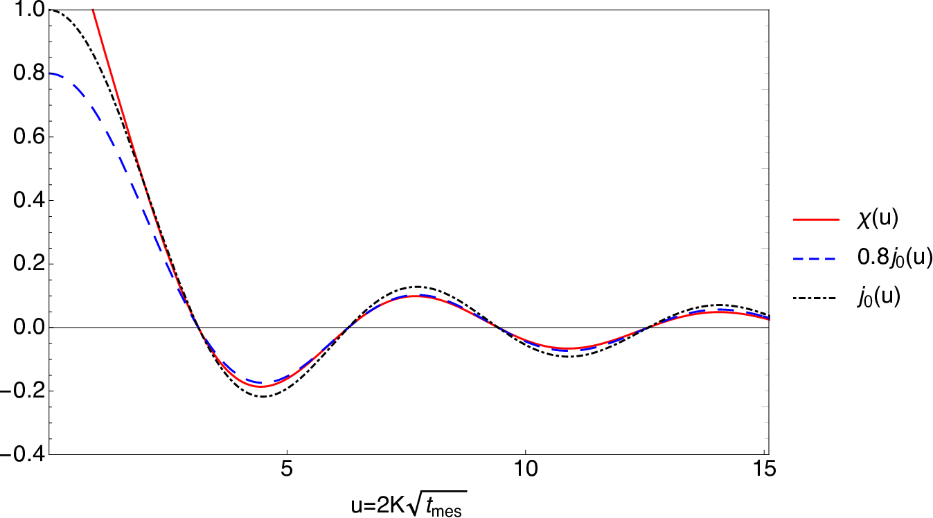
In Fig. (1), we have illustrated the analytical solution (106) for . We have also compared with the solution and the asymptotic solution with the suppression factor suggested in Weinberg:2003ur. The departs from the the solution and approaches the asymptotic solution around as illustrated in Fig. (1).
Now that we have fixed the parameter , the suppression factor of the GW intensity is obtained as . It is worth mentioning that the SGWB also passes through the matter-dominated era until observed at present time. According to an argument given by Weinberg:2003ur, we expect that (106) serves as an initial condition for the subsequent evolution of the gravitational wave amplitude during the matter-dominated era. Therefore, one should still expect the same change in the amplitude during the matter-dominated era.
IV.2 Influence on the polarization of GW
In this part, we provide the system of differential equations given by QBE that describe the time evolution of the GW’s Stokes parameters in the radiation and matter-dominated epochs. To this end, we first define the vector in terms of the gravitational Stokes parameters as the form,
| (107) |
Using this vector and assuming the scaling behavior as , one can represent the evolution equations (65) in the following form:
| (108) | |||||
where
| (109) |
is the symmetric diagonal matrix. Therefore, we have a system of first-order time non-local differential equations that can be numerically integrated in an expanding universe background. Using equation (108) and the same method as in the previous section, we can calculate the parameter during radiation dominance as follows:
| (110) | |||||
where is the V-mode parameter at the end of inflation. Very interestingly, the source term associated with the V-mode polarization of GWs changes sign. Therefore, contrary to the damping effect in the intensity and the linear polarization, the V-mode polarization is amplified by interaction with the medium containing decoupled relativistic fermions. The interaction causes , which, in turn, changes the sign of the parameter. The parity transformation of the interaction Hamiltonian is a clue to identify the sign change of . As it was shown, the interaction Hamiltonian is not invariant under parity transformation and interchanges the right- and left- handed circular polarization modes. Therefore, one can write
| (111) |
where and denote the left- and right- handed V-modes.
V Conclusions
We have discussed that QBE is a powerful and commonly used tool in the investigation of open quantum systems. In the conventional form of the QBE, the Born-Markov approximation is employed. The Markovian QBE is a time-local equation in which one ignores all memory effects. Recent studies show a wide range of applications of the Markovian QBE in the CMB, neutrino physics, and GWs. In this work, we consider memory effects beyond the Markovian approximation and generalize the QBE so that it can be used to describe the non-Markovian processes. Moreover, the conventional form of the Markovian QBE is only applicable to reversible processes. We discussed that for such processes the effective interaction Hamiltonian describing the process at the microscopic scales is invariant under time reversal operation. However, the effective interaction Hamiltonian associated with an irreversible process such as absorption transforms to the effective interaction Hamiltonian of the inverse process under time reversal transformation. We have extended the QBE to a new form that can also describe the irreversible phenomena. Among the many possible applications, in this work, we have used this new equation to explain the phenomenon of gravitational-waves damping during their propagation in an environment consisting of decoupled relativistic fermions using this approach. Using the non-Markovian QBE we obtained an integro-differential equation describing the irreversible dynamics of the reduced graviton system. Here, we computed the time evolution equation of the GW intensity, although we have shown that this equation is quite consistent with the equation previously calculated to explain the damping of the GWs due to free streaming neutrinos in the early universe.
The non-Markovian equations are usually difficult to treat analytically. It would be very interesting to investigate the resulting non-Markovian equations for the density matrix of GWs numerically; however, it is left for future works. We instead considered the limit of the early stage of the radiation-dominated era during which, one can drastically reduce the complexity due to memory effects. The analytical solution for the GW intensity showed that interaction with the ultra-relativistic fermion environment gives rise to a damping effect that induces a suppression in the intensity by a factor more than the condition that there is no contact with the environment.
We then fixed the parameter in such a way that we first obtained an analytical solution for (105), and by comparing our result with the asymptotic solution previously obtained by Weinberg:2003ur, we found . Therefore, the suppression factor during radiation-dominated era was found as .
Additionally, another new aspect of our study, we showed the propagation of a circularly polarized SGWB in an environment of ultra-relativistic fermions that cause an enhancement to the Stokes parameter in contrast with the intensity and the linear polarization. This is because the interaction with the environment changes the handedness of the circularly polarized GWs that in turn causes . This makes an amplification by a factor for the V-mode polarization. However, note that the polarized SGWB also passes through the matter-dominated era until observed at present time. The suppression obtained during the radiation dominated era provides the initial condition for the subsequent evolution during the matter-dominated era.
We can also make a general statement about the amplification of the V-mode polarization due to the coupling of GWs with a background matter field. In general, the linear interaction between the GWs and background matter is characterized through , in which, describes the energy-momentum tensor of matter fields such as photon or dark matter. Inserting this interaction term into the QBE, one can verify that the absorption of a flux of circularly polarized GWs by a background of matter fields will amplify the V-mode polarization if is invariant under the parity transformation.
Acknowledgements.
M.Z. acknowledges financial support by the University of Padova under the MSCA Seal of Excellence @UniPD programme. A.R. acknowledges funding from Italian Ministry of Education, University and Research (MIUR) through the ‘Dipartimenti di eccellenza’ project Science of the Universe. N.B., D.B., and S.M. acknowledge partial financial support by ASI Grant No. 2016-24-H.0 and 2016-24-H.1-2018. M.Z. would like to thank S. Azaele, F. Baldovin, M. Saeedian, and F. Shahbazi for several enlightening and stimulating discussions.Appendix A Calculation of expectation values
A.1 Equal-time operators
In the equilibrium condition, the creation and annihilation operators satisfy equal-time commutation relations
| (112) |
and
| (113) |
Using the above relations, one can calculate the connected equal-time expectation value of operators that is proportional to the density matrix. Before, we would like to emphasize that the correct expression for the expectation values containing all the information are those that involve connected pieces. The connected expectation value is defined as follows:
| (114) |
With this in mind, we begin to calculate the equal-time expectation values for gravitons and ultra-relativistic fermions. First, we calculate the so called two-point equal-time expectation values. In general, the expectation value for gravitons is given by Bartolo:2018igk
| (115) |
Now, using the graviton density operator (36), we have
| (116) |
where is the one-particle graviton state with momentum that is given by
| (117) |
Therefore, using the commutation relation (112), we have
| (118) | |||||
In the same way and using the anti-commutation relation (113), we find
| (119) |

The four-point equal-time expectation values are calculated as follows Kosowsky:1994cy; Danielewicz:1982kk:
| (120) | |||||
where the subscript “c” denotes the sum of all diagrams connected to the external lines. The expectation value of the commutator is calculated as in the following, we write
| (121) | |||||
where is the number of gravitons,
| (122) |
and is assumed to be equal to 1. Therefore, the expected value of four operators is obtained in a similar way to the Wick’s theorem as follows:
| (123) | |||||
where, in the last line, we have kept the linear term in terms of . In Fig. 2, we have diagrammatically shown this expression. In the same manner, we have
| (124) | |||||
where we have assumed that the number of fermions is equal to 1, and therefore, the expectation value of anti-commutation relation is given by
| (125) |
In all of the above expectation values, we can take to be the mesoscopic time .
A.2 Unequal-time expectation values
As was mentioned, it is convenient that in equilibrium quantum field theory, we define the operator algebra for the bosonic and the fermionic creation and annihilation operators by the equal-time canonical commutation and anti-commutation relations. However, for out-of-equilibrium calculations, there are additional complications that do not appear in equilibrium condition. One of them is that in nonequilibrium conditions, we often have to apply time-dependent commutation or anti-commutation relations. In such condition, the Schwinger-Keldysh, in-in or closed-time-path formalism Schwinger:1960qe; Keldysh:1964ud is applied to calculate the evolution and expectation values of observables that usually are in the Heisenberg picture. This formalism has been applied in cosmology, condensed matter problems, and in studying heavy ion collisions (for a detailed discussion, we refer to Refs. Rammer; Kamenevej; Danielewicz:1982kk; Bruus; Berges:2004yj). In particular, it has been used for computing cosmological correlations during cosmological inflation as well as during preheating after inflation, for the dynamics of phase transitions in the early universe, and to study the dynamics of baryogenesis Boyanovsky:1997mq; Chen:2017ryl.
Here, we present a general discussion of the calculation of the time correlation functions. For a system at equilibrium conditions, such correlation functions depend only on the time interval ,
| (126) |
For instance, we compute the non-equal-time expectation values for gravitons under the assumption that gravitons do not interact with the environment,
| (127) | |||||
where is time-dependent Green’s function of creation and annihilation operators, defined as
| (128) |
with the semigroup property that Kamenevej. Therefore, we can write
| (129) |
In the same way, for fermions we have
| (130) |
We are interested in the four-point unequal-time expectation values. As it was assumed, the environment is in the equilibrium state. Therefore, for the fermions, we can write
| (131) | |||||
where, in the last line, we have kept the linear term in terms of . Based on what was discussed, the system of gravitons is in out-of-equilibrium conditions, and therefore, the semigroup condition no longer applies to it. Accordingly, we write the two-point unequal-time expectation value as in the following form:
| (132) |
The four-point unequal-time expectation value is represented in the following form:
| (133) | |||||
In the same manner, we can calculate the following expressions:
| (134) | |||||
and
| (135) | |||||
References
- (1) H. P. Breuer and F . Petruccione, “The Theory of Open Quantum Systems,” Oxford Univ. Press, 2007.
- (2) D. A. Lidar, “Lecture Notes on the Theory of Open Quantum Systems,” [ arXiv:1902.00967].
- (3) I. de Vega and D. Alonso, “Dynamics of non-Markovian open quantum systems,” Rev. Mod. Phys. 89, 015001 (2017) [arXiv:1511.06994v3 ].
- (4) M. Cattaneo, G. L. Giorgi, S. Maniscalco, and R. Zambrini, “Local vs global master equation with common and separate baths: superiority of the global approach in partial secular approximation,” New J. Phys. 21, 113045 (2019) [arXiv:1906.08893 [quant-ph]].
- (5) H. P. Breuer, “Foundations and Measures of Quantum Non-Markovianity,” J. Phys. B: At. Mol. Opt. Phys. 45, 154001 (2012) DOI: 10.1088/0953-4075/45/15/154001 [arXiv:1206.5346 [quant-ph]].
- (6) A. Rivas, A. D. K. Plato, S. F. Huelga, and M. B. Plenio, “Markovian master equations: a critical study,” New Journal of Physics 12, 113032 (2010) [ arXiv:1006.4666 ].
- (7) P. P. Hofer, M. Perarnau-Llobet, L. D. M. Miranda, G. Haack, R. Silva, J. B. Brask, and N. Brunner, “Markovian master equations for quantum thermal machines: local vs global approach,” [arXiv:1707.09211].
- (8) A. Kosowsky, “Cosmic microwave background polarization,” Annals Phys. 246, 49-85 (1996) doi:10.1006/aphy.1996.0020 [arXiv:astro-ph/9501045 [astro-ph]].
- (9) E. Bavarsad, M. Haghighat, Z. Rezaei, R. Mohammadi, I. Motie and M. Zarei, “Generation of circular polarization of the CMB,” Phys. Rev. D 81, 084035 (2010) doi:10.1103/PhysRevD.81.084035 [arXiv:0912.2993 [hep-th]].
- (10) N. Bartolo, A. Hoseinpour, G. Orlando, S. Matarrese and M. Zarei, “Photon-graviton scattering: A new way to detect anisotropic gravitational waves?,” Phys. Rev. D 98, no.2, 023518 (2018) doi:10.1103/PhysRevD.98.023518 [arXiv:1804.06298 [gr-qc]].
- (11) N. Bartolo, A. Hoseinpour, S. Matarrese, G. Orlando and M. Zarei, “CMB Circular and B-mode Polarization from New Interactions,” Phys. Rev. D 100, no.4, 043516 (2019) doi:10.1103/PhysRevD.100.043516 [arXiv:1903.04578 [hep-ph]].
- (12) A. Hoseinpour, M. Zarei, G. Orlando, N. Bartolo and S. Matarrese, “CMB modes from photon-photon forward scattering revisited,” Phys. Rev. D 102, no.6, 063501 (2020) doi:10.1103/PhysRevD.102.063501 [arXiv:2006.14418 [hep-ph]].
- (13) C. Fidler and C. Pitrou, “Kinetic theory of fermions in curved spacetime,” JCAP 06, 013 (2017) doi:10.1088/1475-7516/2017/06/013 [arXiv:1701.08844 [cond-mat.stat-mech]].
- (14) P. Amaro-Seoane et al. [LISA], “Laser Interferometer Space Antenna,” [arXiv:1702.00786 [astro-ph.IM]].
- (15) S. Kawamura, T. Nakamura, M. Ando, N. Seto, K. Tsubono, K. Numata, R. Takahashi, S. Nagano, T. Ishikawa and M. Musha, et al. “The Japanese space gravitational wave antenna DECIGO,” Class. Quant. Grav. 23 (2006), S125-S132 doi:10.1088/0264-9381/23/8/S17
- (16) B. P. Abbott et al. [LIGO Scientific], “Exploring the Sensitivity of Next Generation Gravitational Wave Detectors,” Class. Quant. Grav. 34 (2017) no.4, 044001 doi:10.1088/1361-6382/aa51f4 [arXiv:1607.08697 [astro-ph.IM]].
- (17) B. Sathyaprakash, M. Abernathy, F. Acernese, P. Amaro-Seoane, N. Andersson, K. Arun, F. Barone, B. Barr, M. Barsuglia and M. Beker, et al. “Scientific Potential of Einstein Telescope,” [arXiv:1108.1423 [gr-qc]].
- (18) M. Maggiore, C. Van Den Broeck, N. Bartolo, E. Belgacem, D. Bertacca, M. A. Bizouard, M. Branchesi, S. Clesse, S. Foffa and J. García-Bellido, et al. “Science Case for the Einstein Telescope,” JCAP 03 (2020), 050 doi:10.1088/1475-7516/2020/03/050 [arXiv:1912.02622 [astro-ph.CO]].
- (19) T. Regimbau, “The astrophysical gravitational wave stochastic background,” Res. Astron. Astrophys. 11 (2011), 369-390 doi:10.1088/1674-4527/11/4/001 [arXiv:1101.2762 [astro-ph.CO]].
- (20) M. C. Guzzetti, N. Bartolo, M. Liguori and S. Matarrese, “Gravitational waves from inflation,” Riv. Nuovo Cim. 39 (2016) no.9, 399-495 doi:10.1393/ncr/i2016-10127-1 [arXiv:1605.01615 [astro-ph.CO]].
- (21) C. Caprini and D. G. Figueroa, “Cosmological Backgrounds of Gravitational Waves,” Class. Quant. Grav. 35 (2018) no.16, 163001 doi:10.1088/1361-6382/aac608 [arXiv:1801.04268 [astro-ph.CO]].
- (22) M. Maggiore, “Gravitational wave experiments and early universe cosmology,” Phys. Rept. 331 (2000), 283-367 doi:10.1016/S0370-1573(99)00102-7 [arXiv:gr-qc/9909001 [gr-qc]].
- (23) N. Bartolo, C. Caprini, V. Domcke, D. G. Figueroa, J. Garcia-Bellido, M. C. Guzzetti, M. Liguori, S. Matarrese, M. Peloso and A. Petiteau, et al. “Science with the space-based interferometer LISA. IV: Probing inflation with gravitational waves,” JCAP 12 (2016), 026 doi:10.1088/1475-7516/2016/12/026 [arXiv:1610.06481 [astro-ph.CO]].
- (24) E. Barausse, E. Berti, T. Hertog, S. A. Hughes, P. Jetzer, P. Pani, T. P. Sotiriou, N. Tamanini, H. Witek and K. Yagi, et al. “Prospects for Fundamental Physics with LISA,” Gen. Rel. Grav. 52 (2020) no.8, 81 doi:10.1007/s10714-020-02691-1 [arXiv:2001.09793 [gr-qc]].
- (25) S. W. Hawking, “Perturbations of an expanding universe,” Astrophys. J. 145, 544 (1966).
- (26) S. Gayer and C. F. Kennel, “Possibility Of Landau Damping Of Gravitational Waves,” Phys. Rev. D 19, 1070 (1979).
- (27) A. G. Polnarev, “ The Interaction of VVeak Gravitational Waves with a Gas ,” Sov. Phys. JETP 35, 834 (1972).
- (28) P. Szekeres, “Linearized gravitation theory in macroscopic media,” Annals Phys. 64, 599 (1971).
- (29) S. Weinberg, “Gravitation and Cosmology : Principles and Applications of the General Theory of Relativity,” John Wiley and Sons Inc, 1972.
- (30) S. Weinberg, “Damping of tensor modes in cosmology,” Phys. Rev. D 69, 023503 (2004) doi:10.1103/PhysRevD.69.023503 [arXiv:astro-ph/0306304 [astro-ph]].
- (31) J. R. Pritchard and M. Kamionkowski, “Cosmic microwave background fluctuations from gravitational waves: An Analytic approach,” Annals Phys. 318, 2-36 (2005) [arXiv:astro-ph/0412581 [astro-ph]].
- (32) G. Baym, S. P. Patil and C. J. Pethick, “Damping of gravitational waves by matter,” Phys. Rev. D 96, no.8, 084033 (2017) [arXiv:1707.05192 [gr-qc]].
- (33) Y. Watanabe and E. Komatsu, “Improved Calculation of the Primordial Gravitational Wave Spectrum in the Standard Model,” Phys. Rev. D 73, 123515 (2006) [arXiv:astro-ph/0604176 [astro-ph]].
- (34) D. A. Dicus and W. W. Repko, “Comment on damping of tensor modes in cosmology,” Phys. Rev. D 72, 088302 (2005) doi:10.1103/PhysRevD.72.088302 [arXiv:astro-ph/0509096 [astro-ph]].
- (35) A. Mangilli, N. Bartolo, S. Matarrese and A. Riotto, “The impact of cosmic neutrinos on the gravitational-wave background,” Phys. Rev. D 78 (2008), 083517 doi:10.1103/PhysRevD.78.083517 [arXiv:0805.3234 [astro-ph]].
- (36) L. V. Dall’Armi, A. Ricciardone, N. Bartolo, D. Bertacca and S. Matarrese, “The Imprint of Relativistic Particles on the Anisotropies of the Stochastic Gravitational-Wave Background,” [arXiv:2007.01215 [astro-ph.CO]].
- (37) B. A. Stefanek and W. W. Repko, “Analytic description of the damping of gravitational waves by free streaming neutrinos,” Phys. Rev. D 88 (2013) no.8, 083536 doi:10.1103/PhysRevD.88.083536 [arXiv:1207.7285 [hep-ph]].
- (38) N. Mirón-Granese, “Relativistic viscous effects on the primordial gravitational waves spectrum,” doi:10.1088/1475-7516/2021/06/008 [arXiv:2012.11422 [astro-ph.CO]].
- (39) R. Flauger and S. Weinberg, “Gravitational Waves in Cold Dark Matter,” Phys. Rev. D 97, no.12, 123506 (2018) doi:10.1103/PhysRevD.97.123506 [arXiv:1801.00386 [astro-ph.CO]].
- (40) R. Flauger and S. Weinberg, “Absorption of Gravitational Waves from Distant Sources,” Phys. Rev. D 99, no. 12, 123030 (2019) doi:10.1103/PhysRevD.99.123030 [arXiv:1906.04853 [hep-th]].
- (41) P. Danielewicz, “Quantum Theory of Nonequilibrium Processes. 1.,” Annals Phys. 152, 239-304 (1984).
- (42) H . Bruus and K . Flensberg, “Introduction to many-body quantum theory in condensed matter physics,” Oxford University Press, 2011, 352p.
- (43) J . Rammer, “Quantum field theory of non-equilibrium states,” Cambridge University Press, 2007, 552p.
- (44) A .Kamenevej, “Field theory of non-equilibrium systems,” Cambridge University Press, 2011, 357p.
- (45) J. Berges, “Introduction to nonequilibrium quantum field theory,” AIP Conf. Proc. 739, no.1, 3-62 (2004) doi:10.1063/1.1843591 [arXiv:hep-ph/0409233 [hep-ph]].
- (46) S. Jeon and L. G. Yaffe, “From quantum field theory to hydrodynamics: Transport coefficients and effective kinetic theory,” Phys. Rev. D 53, 5799-5809 (1996) doi:10.1103/PhysRevD.53.5799 [arXiv:hep-ph/9512263 [hep-ph]].
- (47) D. Boyanovsky, I. D. Lawrie and D. S. Lee, “Relaxation and kinetics in scalar field theories,” Phys. Rev. D 54, 4013 (1996) doi:10.1103/PhysRevD.54.4013 [hep-ph/9603217].
- (48) E. A. Calzetta, B. L. Hu and S. A. Ramsey, “Hydrodynamic transport functions from quantum kinetic theory,” Phys. Rev. D 61 (2000) 125013 doi:10.1103/PhysRevD.61.125013 [hep-ph/9910334].
- (49) P. B. Arnold, G. D. Moore and L. G. Yaffe, “Transport coefficients in high temperature gauge theories. 1. Leading log results,” JHEP 0011, 001 (2000) doi:10.1088/1126-6708/2000/11/001 [hep-ph/0010177].
- (50) J. P. Blaizot and E. Iancu, “The Quark gluon plasma: Collective dynamics and hard thermal loops,” Phys. Rept. 359 (2002) 355 doi:10.1016/S0370-1573(01)00061-8 [hep-ph/0101103].
- (51) G. Policastro, D. T. Son and A. O. Starinets, “The Shear viscosity of strongly coupled N=4 supersymmetric Yang-Mills plasma,” Phys. Rev. Lett. 87, 081601 (2001) doi:10.1103/PhysRevLett.87.081601 [arXiv:hep-th/0104066 [hep-th]].
- (52) H. Manshouri, A. Hoseinpour and M. Zarei, “Quantum Boltzmann equation for fermions: an attempt to calculate the NMR relaxation times using the quantum field theory techniques,” [arXiv:2009.01917 [hep-ph]].
- (53) J. S. Schwinger, “Brownian motion of a quantum oscillator,” J. Math. Phys. 2, 407 (1961).
- (54) L. V. Keldysh, “Diagram technique for nonequilibrium processes,” Zh. Eksp. Teor. Fiz. 47, 1515 (1964) [Sov. Phys. JETP 20, 1018 (1965)].
- (55) D . Chruściński, and A .Kossakowski, “Non-Markovian Quantum Dynamics: Local versus Nonlocal”, Phys. Rev. Lett. 104, 070406, (2010) [arXiv:0912.1259] .
- (56) C. P. Burgess, R. Holman, G. Tasinato and M. Williams, “EFT Beyond the Horizon: Stochastic Inflation and How Primordial Quantum Fluctuations Go Classical,” JHEP 03, 090 (2015) doi:10.1007/JHEP03(2015)090 [arXiv:1408.5002 [hep-th]].
- (57) C. P. Burgess, R. Holman and G. Tasinato, “Open EFTs, IR effects \& late-time resummations: systematic corrections in stochastic inflation,” JHEP 01, 153 (2016) doi:10.1007/JHEP01(2016)153 [arXiv:1512.00169 [gr-qc]].
- (58) D. Boyanovsky, “Effective field theory during inflation: Reduced density matrix and its quantum master equation,” Phys. Rev. D 92, no.2, 023527 (2015) doi:10.1103/PhysRevD.92.023527 [arXiv:1506.07395 [astro-ph.CO]].
- (59) D. Boyanovsky, “Effective field theory during inflation. II. Stochastic dynamics and power spectrum suppression,” Phys. Rev. D 93, 043501 (2016) doi:10.1103/PhysRevD.93.043501 [arXiv:1511.06649 [astro-ph.CO]].
- (60) E. Nelson, “Quantum Decoherence During Inflation from Gravitational Nonlinearities,” JCAP 03, 022 (2016) doi:10.1088/1475-7516/2016/03/022 [arXiv:1601.03734 [gr-qc]].
- (61) T. J. Hollowood and J. I. McDonald, “Decoherence, discord and the quantum master equation for cosmological perturbations,” Phys. Rev. D 95, no.10, 103521 (2017) doi:10.1103/PhysRevD.95.103521 [arXiv:1701.02235 [gr-qc]].
- (62) J. Martin and V. Vennin, “Observational constraints on quantum decoherence during inflation,” JCAP 05, 063 (2018) doi:10.1088/1475-7516/2018/05/063 [arXiv:1801.09949 [astro-ph.CO]].
- (63) S. Shandera, N. Agarwal and A. Kamal, “Open quantum cosmological system,” Phys. Rev. D 98, no.8, 083535 (2018) doi:10.1103/PhysRevD.98.083535 [arXiv:1708.00493 [hep-th]].
- (64) G. S. Agarwal, “Open quantum Markovian systems and the microreversibility,” Z. Physik 258, 409 (1973).
- (65) N. A. Voronov, “Gravitational Compton effect and photoproduction of gravitons by electrons,” Sov. Phys. JETP 37, 953 (1973) [Zh. Eksp. Teor. Fiz. 64, 1889 (1973)].
- (66) Itzykson C., Zuber J.-B., “Quantum Field Theory”, McGraw-Hill, 1980.
- (67) V. Berestetskii, L. Pitaevskii, and E. Lifshitz, “Quantum Electrodynamics,” v. 4, Elsevier Science, 2012.
- (68) N. Bartolo, V. Domcke, D. G. Figueroa, J. García-Bellido, M. Peloso, M. Pieroni, A. Ricciardone, M. Sakellariadou, L. Sorbo and G. Tasinato, “Probing non-Gaussian Stochastic Gravitational Wave Backgrounds with LISA,” JCAP 11, 034 (2018) doi:10.1088/1475-7516/2018/11/034 [arXiv:1806.02819 [astro-ph.CO]].
- (69) D. Boyanovsky, D. Cormier, H. J. de Vega, R. Holman and S. P. Kumar, “Out-of-equilibrium fields in inflationary dynamics: Density fluctuations,” NATO Sci. Ser. C 511, 119-194 (1998) doi:10.1007/978-94-011-5046-0_4 [arXiv:hep-ph/9801453 [hep-ph]].
- (70) X. Chen, Y. Wang and Z. Z. Xianyu, “Schwinger-Keldysh Diagrammatics for Primordial Perturbations,” JCAP 12, 006 (2017) doi:10.1088/1475-7516/2017/12/006 [arXiv:1703.10166 [hep-th]].