Performance of Predictive Indoor mmWave Networks with Dynamic Blockers

In this section, we review state-of-the-art approaches that use ML tools to make the blockage prediction of mmWave links. There are three major techniques regarding the data acquisition for training the ML models: (i) using data acquired from the mmWave channel measurements, (ii) utilising complementary data from the Sub-6 GHz channel bands and (iii) collecting data through a camera or radar mounted on top of the mmWave-BS (mmWave-BS).

The authors of [15] consider using multi-link mmWave channel measurements as input data for a Long Short-Term Memory (LSTM) model that predicts the received signal power variations of one of the link in advance. In the single-cell scenario, SNR (SNR) measurements related to both LoS (LoS) and NLoS (NLoS) mmWave links with the serving BS (BS) need to be collected, requiring sweeping the beam towards the NLoS paths directions and interrupting the ongoing data communication with the UE. Moreover, in the multi-cell scenario, the method entails acquiring the SNR measurements from the LoS paths with neighbour BS. In this case, the neighbour BS perform beam sweeping, changing the beams towards UE that are not served, and provide the additional SNR measurements. Thus, integrating the LSTM-based method proposed in [15] into the 5G NR mmWave network operations can be challenging to realise in practice and is still an open research problem. Differently in [16], the authors propose to use unsupervised online learning to predict the mmWave link state. This approach utilises the MPC (MPC) of the mmWave channel as input data for the ML model; however, the predictions are limited to one blocker and rely on its location information, which is usually not available unless, for instance, the blocker is equipped with a localisation device. Another interesting work that relies on data acquired from the mmWave channel measurements is [22], where a UE moving in a vehicle utilises the ML model predictions to select the BS that takes over the communication to avoid the blockage. However, this work is suited for vehicular networks, and we consider this scenario outside the scope of this paper.

Another line of work focuses on using the Sub-6 GHz spectrum bands measurements to observe the rapid variations of the mmWave channel due to the blockage, tens of ms ahead of the blockage event [23]. Following this approach, in [17], the authors propose a DNN (DNN) model that uses the Sub-6 GHz channel measurements to predict the beam state and the optimal beam of the codebook that maximises the achievable rate. Their results show a $90\%$ probability of correct predictions of the mmWave link blockage state. This method is verified with the single-UE scenario, and it is impractical for the SA (SA) mmWave network deployment.

Alternatively, in [19], the authors propose a ML-based predictor of received signal power that uses visual data acquired by a camera pointing to the BS-UE path. Similarly, in [20], the authors use visual data to predict the BS to which handover the connection. Conversely, the RadMAC project is a proof-of-concept that deploys a mmWave radar on top of the mmWave BS [21]. RadMAC tracks with the radar the presence of moving objects, e.g., humans, that can eventually intersect the mmWave link, switching the beam preemptively to a backup link during the blockage events. The applicability of the visual and radar-based systems is proved for the single-UE case, where it is possible to cover the beam path serving the UE with a wide camera angle or with the radar system. However, practical mmWave systems use beam steering with codebook-based transmission to cover multiple UE in the sector, making it more challenging to employ visual and radar-based methods to determine the blockage state for each beam.

In this paper, we propose a novel beam recovery method that is integrated with DNN models to predict blockage events. This method relies on the early indication of the predictions to switch to an alternative beam pair, slightly before the blockage starts to impact the received signal power. Unlike the works [19, 20, 17, 15, 16], we consider extending the blockage prediction method to a more realistic multi-UE setting, enabling us to deploy the ML models into the network to study the data rate performance. Moreover, most of the existing works necessitate extra HW (HW) components, e.g. camera and Sub-6 GHz transceiver, while we rely exclusively on the mmWave channel measurements aggregated from multiple BS. The ML model proposed in [15] uses input data that necessitate additional SNR measurements from the ones already defined in the 5G NR specifications. Instead, we use standard beam-quality measurements reported by the UE to the BS according to the 3GPP NR specification [24].

We consider a mmWave Indoor network with high UE density and multiple BS. We account for BS employing multi-antenna arrays with analog beamforming architecture and codebook-based signal transmission. We incorporate into the 3GPP-based system-level simulator a geometric blockage model (Blockage model B) that ensures consistent results over time, space and frequency components of the channel [25]. The beams intersecting the blocker in locations that are spatially close have beam-quality measurements that follow similar temporal dynamics. Hence, the blocker presence at time $t$ on one beam can indicate the blockage presence on other beams in successive instants of time. Thus, we train a DNN model to predict the beam-specific blockage state, taking as input data the other beams’ measurements exchanged with the neighbour BS through a central controller. Our contributions can be summarised as follows:

1. 1.

   We train a set of beam-specific DNN models with synthetic data generated through a 3GPP-based system-level simulator. The models exclusively use existing beam-quality measurements reported by the UE to the BS as indicated in the 5G NR specifications.

2. 2.

   We propose a novel multi-UE prediction-based method for beam recovery that uses the DNN models’ output to control and initiate the beam switching in advance and complete this operation by the time the mmWave link becomes blocked.

3. 3.

   We validate the prediction-based method by deploying the DNN models online into a 3GPP-based system-level simulator to verify the close match to the performance of an ideal method that has perfect knowledge of the future beam states. We then compare the prediction method to other two cases: i) adopting the beam recovery method based on detection and ii) utilising a fixed beam method. We show that the prediction method switches to a backup beam earlier than the blockage event, and avoids the data rate loss that occurs with the detection method due to the delay in switching to the backup beam and without the switching for the fixed beam method.

4. 4.

   We provide quantitative data rate results of the three methods varying the blocker speed. During blocked time instants, the prediction-based method improves the 25-th percentile of the fixed-beam and detection-based methods data rates by $238\%$ and $24\%$ for blocker speed of $1$ m/s, and by $223\%$ and $82\%$ for blocker speed of $2$ m/s. This shows the benefits of using the prediction-based method for the beam recovery operation, especially for the worst served UE and higher blocker speed.

The remainder of this paper is organised as follows. Section II describes the system model and the mmWave DL (DL) transmission; Section III introduces the beam recovery method based on detection and the beam recovery method based on predictions; Section IV describes the procedure to obtain the beam state predictions; Section V presents the evaluation of the methods under analysis and the main results, and VI summarises the key findings and directions for future research. The following notation is used throughout the paper: boldface lower case and boldface upper case are used for column vectors x and matrices X, respectively. $\textbf{x}^{\mathsf{T}}$ denote the transpose of x. A complex Gaussian random variable $x$ is denoted $x\sim\mathcal{CN}(\mu,\,\sigma^{2})$, where $\mu$ is the mean and $\sigma^{2}$ is the variance. $\left[X\right]$ denotes the Iverson bracket that is defined to be 1 when $X$ is true and 0 when $X$ is false.

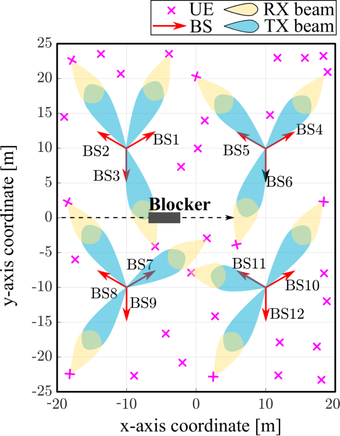
We consider the network layout depicted in Fig. 1 and inspired by the 3GPP Indoor Hot-spot scenario [25, 26], formed by four cell sites deployed on a rectangular grid with an ISD (ISD) of $20$ meters. Each cell site has three sectors, served respectively by three BS oriented with an angle $\theta_{j}$ with $j\in\{1,2,3\}$ and operating at mmWave carrier frequency $f_{c}$, with bandwidth $BW$. The BS in the mmWave network form the set $\mathcal{J}$ with cardinality $J$. We assume a set of $\mathcal{K}$ UE uniformly distributed over a rectangular area of $50$ meters by $40$ meters and we consider dynamic blockers having dimension $w\times h$ moving at speed $v$ in the environment.

Assuming DL transmission, both the BS Tx (Tx) and the UE Rx (Rx) employ UPA (UPA) structures with $M_{Tx}=M_{Tx}^{\rm{V}}\times M_{Tx}^{\rm{H}}$ and $M_{Rx}=M_{Rx}^{\rm{V}}\times M_{Rx}^{\rm{H}}$ antennas spaced half-wavelength, where $M_{Tx}^{\rm{V}}$ and $M_{Rx}^{\rm{V}}$ are the number of Tx and Rx antennas in the vertical direction, and $M_{Tx}^{\rm{H}}$ and $M_{Rx}^{\rm{H}}$ are the ones in the horizontal direction. We assume the BS and UE implement analog beamforming with a single RF (RF) chain, selecting beams from a pre-defined codebook. We denote as $(\theta_{Tx},\phi_{Tx})$ the azimuth and elevation AoD and as $(\theta_{Rx},\phi_{Rx})$ the azimuth and elevation AoA of the Tx and Rx beamforming vectors, respectively. The Tx beamforming vector for UPA can be expressed as $\textbf{b}_{Tx}(\theta_{Tx},\phi_{Tx})=\frac{1}{\sqrt{M_{Tx}^{\rm{H}}M_{Tx}^{\rm{V}}}}\left[1,\dots,e^{-j\pi((M_{Tx}^{\rm{H}}-1)\Theta_{Tx}+(M_{Tx}^{\rm{V}}-1)\Phi_{Tx})}\right]^{\mathsf{T}}$ where $\Theta_{Tx}=\sin\phi_{Tx}\sin\theta_{Tx}$ and $\Phi_{Tx}=\cos\phi_{Tx}$. Similarly, the Rx beamforming vector can be given as $\textbf{b}_{Rx}(\theta_{Rx},\phi_{Rx})=\frac{1}{\sqrt{M_{Rx}^{\rm{H}}M_{Rx}^{\rm{V}}}}\left[1,\dots,e^{-j\pi((M_{Rx}^{\rm{H}}-1)\Theta_{Rx})+(M_{Rx}^{\rm{V}}-1)\Phi_{Rx})}\right]^{\mathsf{T}}$ where $\Theta_{Rx}=\sin\phi_{Rx}\sin\theta_{Rx}$ and $\Phi_{Rx}=\cos\phi_{Rx}$. The beamforming vectors $\textbf{b}_{Tx}$ and $\textbf{b}_{Rx}$ are identified with two beam IDs $l$ and $q$ defined as $l=\{1,\ldots,N_{\mathrm{CB},Tx}\}$ and $q=\{1,\ldots,N_{\mathrm{CB},Rx}\}$, where $N_{\mathrm{CB},Tx}$ and $N_{\mathrm{CB},Rx}$ denote the cardinalities of Tx and Rx codebooks $\mathcal{B}_{Tx}$ and $\mathcal{B}_{Rx}$, respectively. Fig. 2(a) shows the top-down view of the area illuminated by the Tx beams of the BS-3. Each Tx beam of the codebook is steered towards the direction with AoD $(\theta_{Tx},\phi_{Tx})$ as shown in Fig. 2(b), and illuminates a specific area that is marked with a letter-number combination.

Consider the DL of a NR-based system for mmWave cellular communications. The NR standard numerology employs a physical time-frequency resource division corresponding to $14$ OFDM (OFDM) symbols for one TTI (TTI) in the time domain and $12$ consecutive subcarriers in the frequency domain forming a RB (RB) [27]. The system operates with the TDD (TDD) scheme, and each BS uses beam sweeping to time-multiplex multiple UE, serving one UE at a time. At a given time instant $t$, the DL signal transmitted from the BS $j$ to the UE $k$ can be expressed as

where $P_{b}$ is the total power of the BS, $s_{k}(t)$ with $\mathbb{E}[\lvert s_{k}(t)\rvert^{2}]=1$ is the signal transmitted, ${\mathbf{H}}_{j,k}(t)$ represents the impulse response of the three dimensional (3D) SCM (SCM) channel (described in Appendix A), which includes the blockage loss $BL(t)$ (described in Appendix B), $z_{k}(t)\sim\mathcal{CN}(0,\,\sigma^{2}_{z})$ is the noise seen at the $k$-th receiver and $\textbf{b}_{Tx}$ and $\textbf{b}_{Rx}$ are the Tx and Rx beamforming vectors used in forming the beam pair.

In the NR standard, the initial beam pair is established during the Initial Access (IA) phase with the beam management Procedure 1 (P1), consisting of dual Tx and Rx beams sweeping [28]. During this procedure, the BS periodically broadcast SSB, sweeping all the Tx beams over successive SSB and repeating the same operation $N_{\mathrm{CB},Rx}$ times. On the other hand, the UE sweeps the Rx beam every $N_{\mathrm{CB},Tx}$ SSB, while measuring the RSRP (RSRP) for each Tx-Rx beam pair. After the BS-UE sweep all the combinations of Tx and Rx beams, the best beam pair, called primary beam pair, is selected based on the maximum RSRP. Thus the UE associates to the BS providing the maximum RSRP computed with beamforming at both Tx and Rx antennas [29]. The time to sweep all the Tx-Rx beam pairs and complete an entire cycle of SSB transmission can be expressed as¹¹ 1 Each SSB is mapped to $4$ OFDM symbols of the TTI in the time domain and $20$ RB over $275$ RB in the frequency domain [24]. Multiple SSB are grouped in a SS Burst and cover successive TTI. Multiple SS Bursts are referred to as SS Burst Set, which is transmitted in the first half-frame ($5$ ms) and has a periodicity of two NR frames ($T_{SS}=20$ ms). The maximum number of SSB within each SS Burst Set is frequency-dependent and is equal to $L_{\rm{SSB}}=64$ for the Frequency Range 2 (FR2) [30].

where $T_{SS}/2$ is the average time to wait until the subsequent SS Burst Set transmission, assuming that the blockage happens at a time $\bar{t}\sim{\mathcal{U}}[t,t+T_{SS}]$ within the duration of two NR frames.

After the beam-sweeping procedure is completed, the DL transmission between BS $j$ and UE $k$ through the primary beam pair provides a data rate that can be expressed as

where $K_{j}$ represents the number of UE served by the BS $j$ and $I_{j,k}(t)$ represents the inter-cell interference, which can be expressed as $I_{j,k}(t)=\sum_{j^{\prime}\in\mathcal{J}\setminus j}\sqrt{P_{b}}s_{k^{\prime}}(t)\textbf{b}_{Rx}^{\mathsf{T}}{\mathbf{H}}_{j,k}(t)\hat{\textbf{b}}_{Tx}$, where $\hat{\textbf{b}}_{Tx}$ represents the Tx beam directed from BS $j^{\prime}$ to UE $k^{\prime}\neq k$.

In this section, we describe a potential implementation of the current state-of-art method based on a detection threshold to recover the beam when the mmWave links are affected by blockage events, as represented in Fig 3(a). The beam recovery based on the detection (BR-Det) method is considered the benchmark for our studies and operates in three phases. Firstly, it identifies the blockage events when the variations of DL ${\mathrm{SNR}}$ surpass a threshold. Then, it recovers the blocked beams after aligning the backup beam pair with the secondary BS, and finally, it switches back to the primary beam once the blockage is cleared. We define as $\mathit{Th}_{1}$ and $\mathit{Th}_{2}$ two thresholds with values corresponding to $\overline{{\mathrm{SNR}}}_{l}$ minus $70\%$ and $30\%$ of the maximum blockage loss $BL_{max}$, respectively, in line with the procedure adopted in [23].

As shown in Fig. 3(b), whenever the beam is non-blocked, the ${\mathrm{SNR}}$ shows small fluctuations around the average value $\overline{{\mathrm{SNR}}}_{l}$ due to the channel’s multipath components. At the time instant $\bar{t}$ when the blocker starts to intersect the primary beam, the ${\mathrm{SNR}}$ starts to decay rapidly, and the blockage event is detected if ${\mathrm{SNR}}_{l}(t)<\mathit{Th}_{1}$. The beam sweeping procedure follows this event to align the backup beam pair. The time that it takes to handover the communication to the secondary BS from the time when the blockage begins can be expressed as

where $t_{d1}$ is the interval between $\bar{t}$ and the time instant when the ${\mathrm{SNR}}$ decays below the threshold $\mathit{Th}_{1}$, $T_{sweep}$ defined in Eq. (2) denotes the beam sweeping duration to identify the backup beam pair and $T_{HO}$ represents the time interval before the handover to the secondary BS. After switching to the backup beam pair, the data rate of the DL transmission between the secondary BS $j^{\prime}$ and UE $k$ can be expressed as

where $\bar{\textbf{b}}_{Tx}$ and $\bar{\textbf{b}}_{Rx}$ denote the Tx and Rx beamforming vectors of the backup beam pair.

At the end of the blockage event, which lasts for the duration $T_{bl}$, the primary beam ${\mathrm{SNR}}$ returns to values without blockage, i.e. $\overline{{\mathrm{SNR}}}_{l}$, and the UE switches back to the primary beam pair. The time that it takes to handover the communication back to the BS $j$ from the time when the blockage ends can be expressed as

where $t_{d2}$ is the interval between the time instant $\bar{t}+T_{bl}$, representing the end of the blockage and the time instant when ${\mathrm{SNR}}(t)>\mathit{Th}_{2}$, and $T_{HO}$ is the time before the handover to BS $j$.

The data rate of UE $k$ obtained while adopting the BR-Det method can be expressed as

In this section, we propose a novel beam recovery method based on predictions (BR-Pre) capable of switching to the backup beam pair, before the blocker affects the quality of the ongoing communication over the primary beam pair.

Firstly, we define the prediction window $\eta$ to be larger than the beam sweeping duration $T_{sweep}$ and the handover period $T_{HO}$, i.e. $\eta>T_{sweep}+T_{HO}$. The BR-Pre method evaluates at the beginning of the prediction window, i.e. at the time $t-\eta$, the beam state predictions $\hat{S}_{l}$ indicating whether the blockage is going to obstruct the primary beam after the end of the prediction window $\eta$, at time $t$. If the beam is predicted as non-blocked, i.e. $\hat{S}_{l}(t)=0$, the BR-Pre method continues using the primary beam pair. Differently, when the beam is predicted as blocked, i.e. $\hat{S}_{l}(t)=1$, the BR-Pre method uses this early indication to start the beam sweeping procedure in advance to establish the backup beam pair.⁵⁵ 5 We recall that the beam sweeping procedure can be performed during data transmission as it only uses a partial set of RB and OFDM symbols in the TTI where the SSB transmission occurs.

At the end of the prediction window, the BR-Pre method switches to a newly computed backup beam pair and the data rate of the DL transmission between the secondary BS $j^{\prime}$ and UE $k$ can be expressed as in Eq. 6. We want to emphasise that the advantage of the BR-Pre against the BR-Det method is that at the time of the beam switching (assuming the beam state predictions are correct, i.e. $\hat{S}_{l}(t)={S}_{l}(t)$) the primary beam ${\mathrm{SNR}}$ has not yet dropped since the beam switching happens at the end of the prediction window and before the blockage begins, while with the BR-Det method described in Sec. III-A, the beam switching happens with a delay $\beta_{1}$ after the blockage begins.

During the blockage, the BR-Pre method continues to evaluate the predictions of the beam $l$, and if the state becomes non-blocked, i.e. $\hat{S}_{l}(t)=0$, the BR-Pre switches back to the primary beam pair. The data rate of UE $k$ obtained while adopting the BR-Pre method can be expressed as

In this subsection, we introduce a pre-processing step that extracts a subset of beams to use for the predictions considering the cross-correlation between the ${\mathrm{SNR}}$ time series of different beams. This procedure is motivated by two observations. First, the network presents many beams that will be irrelevant for predicting a specific beam state. This could needlessly complicate the training process without delivering any improvement. Second, since correlated beams are most likely spatially close, they also belong to the same BS or neighbour BS. Therefore, we can also optimise the exchange of information among BS to limit the use of a central server.

Let us consider the pair of Tx beams $l$-$l^{\prime}$. The delay between $l$ and $l^{\prime}$ is estimated as $\delta_{l,l^{\prime}}=\argmax_{\forall\tau}R_{l,l^{\prime}}(\tau)$, where $R_{l,l^{\prime}}(\tau)=\sum_{t=0}^{T}{\mathrm{SNR}}_{l}(t){\mathrm{SNR}}_{l^{\prime}}(t-\tau)$ is the cross-correlation between the ${\mathrm{SNR}}$ time series of $l$ and the ${\mathrm{SNR}}$ time series of $l^{\prime}$ defined over the time window $[0,T]$, where $T$ is the total observation time. We estimate the delays between $l$ and all the other beams $l^{\prime}\in\mathcal{B}~\setminus~l$, where $\mathcal{B}=\{1,2,\ldots,(N_{\mathrm{CB},Tx}\times J)\}$ represents the set of all the network’s beams and $B=N_{\mathrm{CB},Tx}\times J$ is the total number of beams in the network. Then, we pick the $L$ beams that have the lowest delays in absolute value, indicating that they are spatially close to beam $l$ and we define a set $\mathcal{C}_{l}=\{c_{1},c_{2},\ldots,c_{L}\}$, which contains the beams to use for predicting the state of beam $l$. In Algorithm 1, we describe the procedure in details.

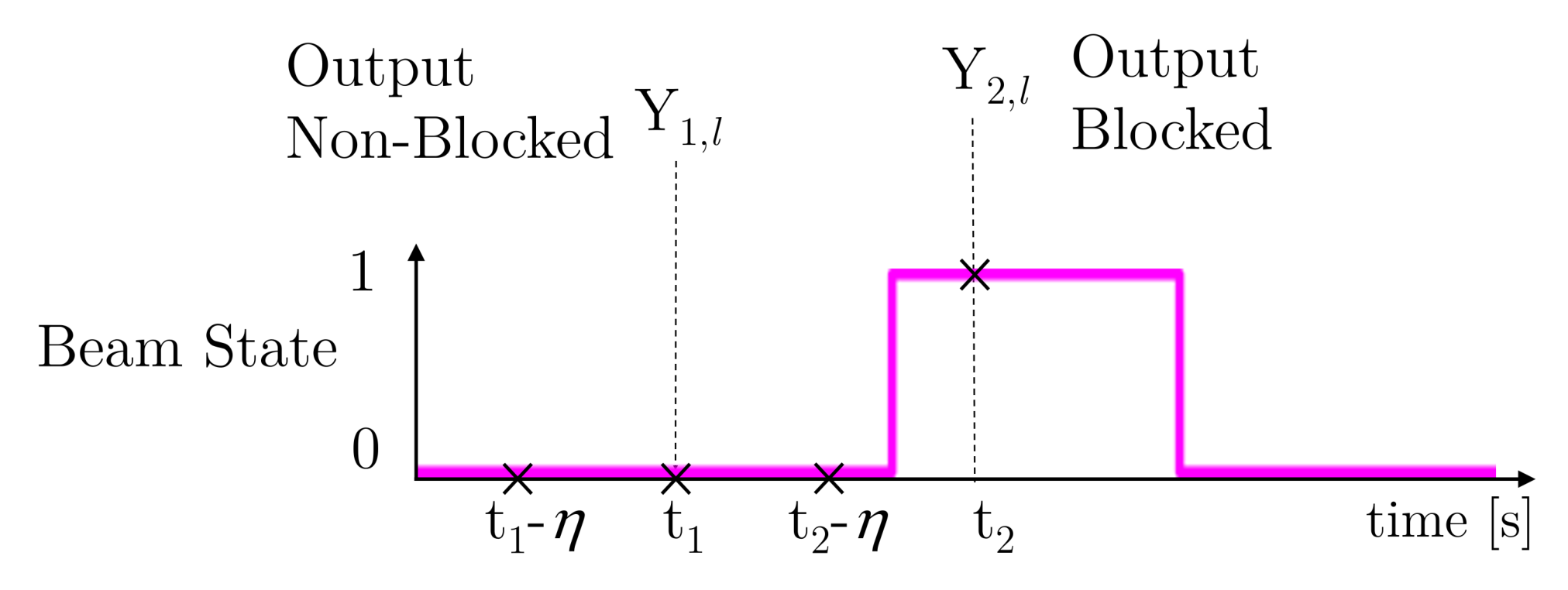
We consider a dataset formed by $N$ samples, where the $n$-th sample of the dataset is organised into input/output vectors generated as follows:

• •

  Input: let us define as ${\mathbf{v}}_{l}=[{\mathrm{SNR}}_{l}[t-\eta-(\epsilon-1)],{\mathrm{SNR}}_{l}[t-\eta-(\epsilon-2)],\ldots,{\mathrm{SNR}}_{l}[t-\eta]]^{\mathsf{T}}$ the vector containing $\epsilon$ samples of the ${\mathrm{SNR}}$ for beam $l$. We assume that the ${\mathrm{SNR}}$ measurements from the beams in the set $C_{l}=\{c_{1},c_{2},\ldots,c_{L}\}$ are exchanged with the BS through a central server. These data are also represented for each beam $l^{\prime}\in\mathcal{C}_{l}$ with a vector ${\mathbf{v}}_{l^{\prime}}=[{\mathrm{SNR}}_{l^{\prime}}[t-\eta-(\epsilon-1)],{\mathrm{SNR}}_{l^{\prime}}[t-\eta-(\epsilon-2)],\ldots,{\mathrm{SNR}}_{l^{\prime}}[t-\eta]]^{\mathsf{T}}$ containing $\epsilon$ samples of the ${\mathrm{SNR}}$. Thus, the input is defined as ${\mathbf{X}}_{n,l}=\left[{\mathbf{v}}_{l},{\mathbf{v}}_{c_{1}},{\mathbf{v}}_{c_{2}},\ldots,{\mathbf{v}}_{c_{L}}\right]\in{\mathbb{R}}^{\epsilon\times(L+1)}$ and aggregates the ${\mathrm{SNR}}$ measurements of $L+1$ beams altogether.

• •

  Output: the output is constituted by a variable $Y_{n,l}$ set to $1$ (blocked) or $0$ (non-blocked) according to the GT state of the beam $l$ at time instant $t$. We obtain this information from the simulation environment. We set the label to $1$ (blocked), when the blocker intersects the LoS path between BS and UE. Conversely, we set the label to $0$ (non-blocked) when there is no intersection.

If the beam is assigned to multiple UE, we fill in the input vector with the median ${\mathrm{SNR}}$ and output variable corresponding to the most frequent label inside the UE group. If there are no UE assigned to a beam, the corresponding ${\mathrm{SNR}}$ measurement cannot be recorded, and the input’s entries are filled with a constant ${\mathrm{SNR}}$ (in our simulations, we use $60$ dB) outside the range of the possible ${\mathrm{SNR}}$ values.

Figs. 5(a) and 5(b) show a simplified scenario where a set of beams shown on the left side of the BS is used to predict the state of the beam $l$, depicted with the line pattern (magenta) on the right side of the BS. The entries of the dataset are formed by associating the inputs ${\mathbf{X}}_{1,l}$ and ${\mathbf{X}}_{2,l}$ to the values of the GT state $Y_{1,l}$ and $Y_{2,l}$ reported in Fig. 5(c). The two different examples show how the input data changes depending on the value of the ground-truth. In the first example, depicted in Fig. 5(a), the ${\mathrm{SNR}}$ measurements (within the sliding window of length $\epsilon$) show small variations indicating that the set of beams at the time $t_{1}-\eta$ is not affected by the blocker. This behaviour suggests that also the magenta beam is likely not affected by the blocker at the instant $t_{1}$. Indeed, as shown in Fig. 5(c), the GT state corresponds to the non-blocked value, i.e. $Y_{1,l}=0$. On the other hand, in the second example, depicted in Fig. 5(b), the ${\mathrm{SNR}}$ measurements show large drops for the set of beams at the time $t_{2}-\eta$, indicating that the magenta beam is likely affected by the blocker movement at the time $t_{2}$. This is confirmed by the GT state $Y_{2,l}=1$, which corresponds to the blocked value.

For training the ML model, we employ a DNN structure constituted by: i) an input layer with $\epsilon\times(L+1)$ inputs, ii) two hidden layers, and iii) a softmax function as output layer. We train each DNN model with Adam (Adam) optimiser adopting He weights initialisation and ReLu (ReLu) activation functions [32, 33].

During the training, we divide the dataset into mini-batch of size $N_{bs}$ assuming a constant learning rate. We repeat the training for several epochs to find the set of model parameters denoted as ${\mathbf{\Omega}}_{l}$ that minimises the cross-entropy loss, given the set of inputs ${\mathbf{X}}_{1,l},\ldots,{\mathbf{X}}_{N_{bs},l}$ and the set of GT labels $Y_{1,l},\ldots,Y_{N_{bs},l}$. The lower is the loss of the model output compared to the ground-truth, and the better is the model.

Moreover, since the time spent by the beam in the non-blocked state prevails over the time spent in the blocked state, the dataset presents a skewed distribution towards the non-blocked class that implies a class imbalance problem [35]. To re-balance the loss, we assign a higher weight to the cross-entropy loss computed for the rare class (blocked) and a lower weight to the cross-entropy loss computed for the dominant class (non-blocked). The weighted formulation of the cross-entropy loss can be expressed as

where $\widehat{Z}_{n,l}$ is the output of the softmax function and indicates the likelihood for the beam $l$ to be in the state non-blocked or blocked. Moreover, the class weights $\mu_{1,l}$ and $\mu_{2,l}$ are computed as the inverse of the number of training samples for each class, i.e. $\mu_{1,l}=N/{\sum_{n=1}^{N}\left[Y_{n,l}=0\right]}$ and $\mu_{2,l}=N/{\sum_{n=1}^{N}\left[{Y_{n,l}=1}\right]}$, respectively.

Table I reports the training configurations and the list of hyper-parameters such as the number of hidden neurons, learning rate and L2 regularisation with the initial configuration values we adopted for the training. Note that the L2 regularisation incorporates in the loss function depicted in Eq. (10) a penalty term on the neuron weights, which reduces the overfit to the training dataset and improves the generalisation of the DNN model [36].

The preparation of the dataset used for training the DNN models involves several steps that entail the setup of the 3GPP-based system-level simulator, including the setup of the blocker’s movement, the generation of a beam-specific dataset, the selection of the validation metric and the configuration of the prediction parameters. Now we discuss each of these steps:

1) Simulation setup: we take a drop-based approach to generate synthetic data utilising a detailed and calibrated system-level simulator that implements 3GPP 3D SCM for the 0.5-100 GHz spectrum [25]. We configure the simulator according to the list of parameters reported in Table II of Appendix C. We simulate the mmWave network shown in Fig. 1, placing the BS on a rectangular grid and the UE in random positions, which are kept fixed between drops. We assume time-invariant large-scale channel parameters (LSPs) such as delay spread, AoD and AoA spread, Rician K-factor, shadow fading (SF) and pathloss, for the duration of the drop $T$. Additionally, at each simulation step within a drop, we assume i) time-variant blockage loss $BL(t)$ due to the blocker’s movement and ii) time-variant small-scale channel parameters (SSPs), e.g. power, phase, delay, AoA and AoD for each MPC, that change independently between simulation steps due to the variations of the multipath fading. We fix the network drop duration to $T=40$ s, and we consider an interval $\Delta t=200$ ms to update the channel ${\mathbf{H}}$ between the simulation steps. We compute every BS-UE link’s channel and the DL ${\mathrm{SNR}}$ for each beam and for all the RB of the system bandwidth at each simulation step.

2) Dynamic blockage generation: to model the blockage loss, we adopt the Blockage Model B that is incorporated within the 3GPP 3D SCM. Compared to the stochastic Blockage Model A [37], the deterministic Blockage Model B supports spatial consistency, which enables to simulate the smooth and continuous-time evolution of the blockage effect while capturing the correlated behaviour of the blockage loss for UE located closely [25]. As a case study, we consider the presence of one blocker at a time moving in the network scenario. The blocker has dimensions 2 m $\times$ 3 m and constant speed $v$ selected randomly between two values $1$ m/s and $2$ m/s, in line with the recommended blocker parameters listed in [25]. The initial position is set at the x-y coordinates $(-20,0)$ m, corresponding to the left side of the network layout, and it moves along the x-axis line from left to right till reaching x-y coordinates $(20,0)$. When the blocker arrives at the right side of the network layout, it regenerates at the initial position and repeats the same movement.⁶⁶ 6 This use case is indicated for scenarios such as future industrial factories, where Automated Guided Vehicles (AGVs) or industrial robots, may maintain similar movement patterns and follow a dedicated pathway in the factory corridor.

3) Beam-specific dataset: we generate a training dataset per beam, collecting ${\mathrm{SNR}}$ measurements over time for successive simulation steps and repeat the same process for $100$ network drops, including both values of the blocker speed in the same dataset. For instance, the beam $(\rm{C},2)$ dataset has $\mathord{\sim}1.5$ million samples divided between $\mathord{\sim}{80}$ thousand samples for the blocked class and $\mathord{\sim}1.42$ million samples for the non-blocked class. We split this data according to the commonly used ratio of $80$/$20$ to use $80\%$ of the dataset for training the DNN model and the remaining $20\%$ of the dataset to validate the DNN model performance. During the training, we consider mini-batch of size $N_{bs}=1000$ samples and $50$ training epochs.

4) Validation metrics: as shown before for the beam $(\rm{C},2)$, the number of non-blocked samples significantly outweighs the blocked samples. Thus, for our specific scenario, we validate the DNN models adopting the F1-score metric, which is more appropriate than the Accuracy metric for the problems presenting highly unbalanced class-distribution [35]. The F1-score combines through the harmonic mean Precision and Recall and can be calculated as $\text{F1-score}=\frac{2\times\text{Precision}\times\text{Recall}}{\text{Precision}+\text{Recall}}$. Recall indicates the proportion of actual blocked samples ( TP (TP) cases) over all the blocked samples (TP and FN (FN) cases), and is calculated as $\text{Recall}=\frac{\rm{TP}}{\rm{TP}+\rm{FN}}$. Conversely, Precision indicates the proportion of actual blocked samples among all predicted blocked samples (TP and FP (FP) cases) and is calculated as $\text{Precision}=\frac{\rm{TP}}{\rm{TP}+\rm{FP}}$.

5) Prediction parameters: we fix the prediction window length to $\eta=400$ ms, which is larger than the combined duration of the beam sweeping procedure, i.e. $T_{sweep}=330$ ms, and the handover time, i.e. $T_{HO}=50$ ms [38]. We adjusted the DNN models input size after several training attempts, which led us to use the number of input beams $L=5$ and set the sliding window duration to $\epsilon=2$ s.

In Fig. 6, we show the training and validation results of the DNN models taking as an exemplary reference BS-3 and several of its blocked beams having different azimuth and elevation AoD. Nevertheless, the same process can be repeated without loss of generality for other BS of the network. The training process highlighted that the DNN models of different beams should be tuned separately. In other words, it is not possible to use the same set of hyper-parameters for all DNN. Hence, we perform an independent validation of the DNN models beam by beam. During the training, we change the L2 regularisation value in the range $\{10^{-5}-10^{-1}\}$ to reduce the overfitting. We measure the performance of each beam for five different random initialisation of the neuron weights. Then, we save the model that returns the maximum F1-score performance on the validation data.

Looking at the results in Fig. 6, we report between parenthesis the value of L2 regularisation hyper-parameter that corresponds to the model attaining the best F1-score. Then, we report Recall, Prediction and F1-score results measured on the validation data and the F1-score result measured on the training data. Firstly, most of the beams show Recall validation performance higher than Precision validation performance. This is due to the class weights applied to the loss function, shown in Eq. (10), which penalises more the FN errors than the FP errors. This setting increases the probability of predicting the blockage correctly but is likely to make more FP errors for the non-blocked samples. Thus the models achieve high Recall while sacrificing their Precision. Secondly, Fig. 6 shows that the beam achieves F1-score validation results close to the F1-score training results. This indicates the models’ ability to generalise from the training data to other data generated with the simulator assuming different network drops, the same blocker size/trajectory and blocker speed that can vary randomly between the values of $1$ m/s and $2$ m/s, as we will see in Sec. V-C and Sec. V-E, where we deploy the DNN models into the simulator.

In this section and in the one that follows, we test the DNN models online into the system-level simulator by generating ten different network drops as compared to the ones used in the training dataset with the blocker moving at the speeds $1$ m/s, and other ten network drops with the speed of $2$ m/s. Fig. 7 shows the ${\mathrm{SNR}}$ measurements’ evolution in the time domain for two Tx beams of the BS-3’s codebook with the blocker moving at the speeds $1$ m/s and $2$ m/s. These results highlight the BR-Pre behaviour over time and show the differences between the BR-Pre method, the BR-Det method and the case where the transmission continues to be handled by the primary beam. Focusing on Fig. 7(a), the bottom part shows the GT and predicted primary beam states. It is worth recalling that the GT state is determined by considering the intersection between the direct path that joins Tx and Rx and the rectangular screen modelling the blocker, as described in Section IV-B. Conversely, the upper part of Fig 7(a) shows the corresponding evolution of the measured ${\mathrm{SNR}}$.

During the non-blocked time instants, the backup beam pair shows a lower ${\mathrm{SNR}}$ than the primary beam pair because it is established with a secondary BS. Differently, before the primary beam enters into a blocked state (as indicated by the ground-truth state in the bottom part of the figure), the ${\mathrm{SNR}}$ of the primary beam pair starts decreasing, while the ${\mathrm{SNR}}$ of the backup beam pair remains stable, providing a higher ${\mathrm{SNR}}$ than the primary beam for the following blocked time instants. The BR-Det method switches to the backup beam with a delay $\beta_{1}$ that considers the beam sweeping interval initiated after detecting the blockage. Thus, as shown in Fig. 7(a), during the time interval $7.8$ s - $8.4$ s, the BR-Det experiences a significant drop of the ${\mathrm{SNR}}$ that is recovered only after switching to the backup beam at the time $t=8.4$ s.

On the other hand, as shown in the two Figs. 7(a) and 7(b), the BR-Pre method uses the DNN models predictions that infer the beam state $\eta$ time instants ahead of the time instant $t$. Thus, the BR-Pre method initiates the beam sweeping procedure at the beginning of the prediction window, i.e. at the time $t-\eta$. After the end of the prediction window, i.e. at the time $t$, when the ${\mathrm{SNR}}$ of the primary beam pair starts decreasing, the BR-Pre method has already switched to the backup beam and avoids the ${\mathrm{SNR}}$ drop that happens with the BR-Det method. However, as shown in Fig. 7(a) during the time intervals $7.2$ s - $7.6$ s and $9.8$ s - $10.4$ s and in Fig. 7(b) for the interval $27.4$ s - $27.6$ s the BR-Pre method presents a ${\mathrm{SNR}}$ lower than the BR-Det method as the BR-Pre method uses the backup beam instead of the primary beam. This is caused by the FP errors associated with the cases when the DNN models wrongly predict the beam state as blocked when there is no blockage present. We will show later in Sec. V-D the limited impact of these errors on the data rate performance.

In this section, we show the CDF of the UE data rate offered by our exemplary BS-3 with the blocker moving at speeds $1$ m/s and $2$ m/s. In Fig. 8, we show the performance of the BR-Pre method, which uses the DNN models to make online predictions, as explained in Sec. III-B, and we compare the results to the GT method, representing the upper bound rate achievable when Eq. (9) has perfect knowledge of the future beam states. During the blocked intervals, the CDF of Fig. 8(a) show that for the blocker speed of $1$ m/s, the median BR-Pre data rate performance reaches $92\%$ of the GT method performance, while for the blocker moving at 2 m/s, the BR-Pre method achieves $89\%$ of the GT data rate. The differences between BR-Pre and GT method data rates are due to the FN errors that cause the BR-Pre method to use the primary beam during the blocked time instants. Nevertheless, these results show that the BR-Pre method almost matches the GT method data rate performance.

On the other hand, Fig. 8(b) shows the CDF of the BR-Pre method data rate achieves $96\%$ of the median GT data rate during non-blocked time instants due to the impact of the FP errors. The FP errors cause switching to the backup beam during the non-blocked intervals while the primary beam has a larger SNR than the backup beam. Fig. 8(b) show that the different CDF curves overlap, meaning that the FP errors observed in Fig. 7 do not significantly impact the data rate performance of the BR-Pre method. Overall, the results in Figs. 8(a) and 8(b) indicate that the DNN models, when deployed online, generalise well for both the blocker speeds.

In this section, we compare the results between the proposed BR-Pre method, the benchmark BR-Det method reported in Sec. III-A and the beam fixed (BF) method, presenting the lower bound rate achievable using the primary beam pair. The CDF in Fig. 9(a) show that the BR-Pre method outperforms the BR-Det and BF methods during the blocked time instants, especially for the higher blocker speed. These results are explained as follows. We recall that the delay $\beta_{1}$ for detecting and switching the beam penalises the BR-Det data rate at the start of the blockage event. On the other hand, as shown before in Sec. V-D, the BR-Pre method performance reaches $92\%$ and $89\%$ of the GT data rate due to the low number of FN errors. Overall, the DNN models wrong predictions have a minor impact on the data rate performance than the delay introduced for detecting the blockage and switching the beam. At a higher blocker speed, the beam switching happens more often, and the BR-Det data rate is penalised by the delay more times than with the blocker moving at 1 m/s, leading to a more significant difference to the BR-Pre results, as represented in Fig. 9(a). Additionally, Fig. 9(b) shows that in the non-blocked time instants, the BR-Pre data rates slightly deteriorate compared to the BR-Det data rate by $4\%$ and $3\%$ at the median of the two speeds CDF, and by $6\%$ and $5\%$ at the 25-th percentile of the two speeds CDF. These results show that during non-blocked time instants, the BR-Pre method performance difference to the BR-Det data rate, caused by the FP errors, are marginal.

In the remainder of this section, we take a deeper look at the data rate performance focusing on the lower part of the CDF presented in Fig. 9, as the worst served UE are most likely to suffer in blocked time instants to meet the requirement of the most demanding applications. Focusing on the 25th percentile results at blocker speed $1$ m/s shown in Fig. 10(a), the BR-Det and BR-Pre methods improve the BF data rate by $172\%$ and $238\%$ respectively and with BR-Pre outperforming BR-Det by $24\%$. Similarly, looking at 25th percentile results of Fig. 10(b) with the blocker moving at the speed of $2$ m/s, the BR-Det and the BR-Pre methods improve the BF method data rate by $77\%$ and $223\%$, respectively. The advantage of BR-Pre over BR-Det increases, and it is assessed at $84\%$. Note that the advantage offered by the BR-Pre method over the BR-Det one is more evident at the higher speed, as the reaction time of BR-Det does not scale with the higher frequency of the blockage events and their shorter duration, thus, by the time the method triggers the switch to the backup beam pair, the drop in the signal level caused by the blockage is either about to finish or already finished. In contrast, the BR-Pre data rate performance does not depend on the blocker speed, showing how predicting in advance the blockage occurrence is effective in indoor factory network deployments.

Similar considerations apply for the median and the 75th percentiles of CDF with blocker speed of $2$ m/s showing $39\%$ and $32\%$ performance gains of our proposed prediction method over the detection one.

References

- [1] O. Simeone, “A very brief introduction to machine learning with applications to communication systems,” IEEE Transactions on Cognitive Communications and Networking, vol. 4, no. 4, pp. 648–664, 2018.
- [2] L. Gavrilovska, V. Atanasovski, I. Macaluso, and L. A. DaSilva, “Learning and reasoning in cognitive radio networks,” IEEE Communications Surveys Tutorials, vol. 15, no. 4, pp. 1761–1777, 2013.
- [3] Y. Sun, M. Peng, Y. Zhou, Y. Huang, and S. Mao, “Application of machine learning in wireless networks: Key techniques and open issues,” IEEE Communications Surveys Tutorials, vol. 21, no. 4, pp. 3072–3108, 2019.
- [4] S. Rangan, T. S. Rappaport, and E. Erkip, “Millimeter-wave cellular wireless networks: Potentials and challenges,” Proceedings of the IEEE, vol. 102, no. 3, pp. 366–385, 2014.
- [5] A. Ghosh, T. A. Thomas, M. C. Cudak, R. Ratasuk, P. Moorut, F. W. Vook, T. S. Rappaport, G. R. MacCartney, S. Sun, and S. Nie, “Millimeter-wave enhanced local area systems: A high-data-rate approach for future wireless networks,” IEEE Journal on Selected Areas in Communications, vol. 32, no. 6, pp. 1152–1163, 2014.
- [6] T. Bai and R. W. Heath, “Coverage and rate analysis for millimeter-wave cellular networks,” IEEE Transactions on Wireless Communications, vol. 14, no. 2, pp. 1100–1114, 2015.
- [7] J. Kibiłda et al., “Indoor millimeter-wave systems: Design and performance evaluation,” Proceedings of the IEEE, vol. 108, no. 6, pp. 923–944, 2020.
- [8] S. Kutty and D. Sen, “Beamforming for millimeter wave communications: An inclusive survey,” IEEE Communications Surveys & Tutorials, vol. 18, no. 2, pp. 949–973, 2016.
- [9] G. R. MacCartney, T. S. Rappaport, and S. Rangan, “Rapid fading due to human blockage in pedestrian crowds at 5G millimeter-wave frequencies,” in 2017 IEEE Global Communications Conference (GLOBECOM), 2017, pp. 1–7.
- [10] C. Slezak, M. Zhang, M. Mezzavilla, and S. Rangan, “Understanding end-to-end effects of channel dynamics in millimeter wave 5G new radio,” in 2018 IEEE 19th International Workshop on Signal Processing Advances in Wireless Communications (SPAWC), 2018, pp. 1–5.
- [11] R. Ford, M. Zhang, M. Mezzavilla, S. Dutta, S. Rangan, and M. Zorzi, “Achieving ultra-low latency in 5G millimeter wave cellular networks,” IEEE Communications Magazine, vol. 55, no. 3, pp. 196–203, March 2017.
- [12] 3GPP Technical Specification (TS) 38.321, “NR; Medium Access Control (MAC) protocol specification,” Version 16.0.0, Apr. 2020.
- [13] Y. M. Tsang and A. S. Y. Poon, “Detecting human blockage and device movement in mmWave communication system,” in 2011 IEEE Global Telecommunications Conference (GLOBECOM) 2011, 2011, pp. 1–6.
- [14] M. Jasim, M. Ababneh, N. Siasi, and N. Ghani, “Hybrid beamforming for link recovery in millimeter wave communications,” in 2018 IEEE 19th Wireless and Microwave Technology Conference (WAMICON), 2018, pp. 1–4.
- [15] S. H. A. Shah, M. Sharma, and S. Rangan, “LSTM-based multi-link prediction for mmwave and Sub-THz wireless systems,” in ICC 2020 - 2020 IEEE International Conference on Communications (ICC), 2020, pp. 1–6.
- [16] M. Zarifneshat, L. Xiao, and J. Tang, “Learning-based blockage prediction for robust links in dynamic millimeter wave networks,” in 2019 16th Annual IEEE International Conference on Sensing, Communication, and Networking (SECON), June 2019, pp. 1–9.
- [17] M. Alrabeiah and A. Alkhateeb, “Deep learning for mmWave beam and blockage prediction using Sub-6 GHz channels,” IEEE Transactions on Communications, vol. 68, no. 9, pp. 5504–5518, 2020.
- [18] Y. Wang, A. Klautau, M. Ribero, A. C. K. Soong, and R. W. Heath, “MmWave vehicular beam selection with situational awareness using machine learning,” IEEE Access, vol. 7, pp. 87 479–87 493, 2019.
- [19] T. Nishio, H. Okamoto, K. Nakashima, Y. Koda, K. Yamamoto, M. Morikura, Y. Asai, and R. Miyatake, “Proactive received power prediction using machine learning and depth images for mmWave networks,” IEEE Journal on Selected Areas in Communications, vol. 37, no. 11, pp. 2413–2427, 2019.
- [20] Y. Koda, K. Nakashima, K. Yamamoto, T. Nishio, and M. Morikura, “Handover management for mmWave networks with proactive performance prediction using camera images and deep reinforcement learning,” IEEE Transactions on Cognitive Communications and Networking, vol. 6, no. 2, pp. 802–816, 2020.
- [21] L. Simić, J. Arnold, M. Petrova, and P. Mähänen, “RadMAC: Radar-enabled link obstruction avoidance for agile mm-wave beamsteering,” in Proceedings of the 3rd Workshop on Hot Topics in Wireless, 2016, pp. 61–65.
- [22] A. Alkhateeb, I. Beltagy, and S. Alex, “Machine learning for reliable mmWave systems: blockage prediction and proactive handoff,” in 2018 IEEE Global Conference on Signal and Information Processing (GlobalSIP), 2018, pp. 1055–1059.
- [23] Z. Ali, A. Duel-Hallen, and H. Hallen, “Early warning of mmWave signal blockage and AoA transition using sub-6 GHz observations,” IEEE Communications Letters, vol. 24, no. 1, pp. 207–211, 2020.
- [24] 3GPP Technical Specification (TS) 38.300, “NR; Overall description; Stage-2,” Version 16.1.0, Apr. 2020.
- [25] 3GPP Technical Report (TR) 38.901, “Study on channel model for frequencies from 0.5 to 100 GHz,” Version 16.1.0, Jan. 2020.
- [26] 3GPP RT-170019, “Summary of Email Discussion [ITU-R AH 01] Calibration for Self-Evaluation,” 3GPP TSG RAN ITU-R ad hoc, Dec. 2017.
- [27] 3GPP Technical Specification (TS) 38.211, “NR; Physical channels and modulation,” Version 16.1.0, Apr. 2020.
- [28] 3GPP Technical Report (TR) 38.802, “Study on new radio access technology physical layer aspects,” Version 14.2.0, Sep. 2017.
- [29] 3GPP R1-1802446, “Discussion on the RSRP calculation,” China Telecom, Feb. 2018.
- [30] 3GPP Technical Specification (TS) 38.213, “NR; Physical layer procedures for control,” Version 16.1.0, Apr. 2020.
- [31] M. Giordani, M. Polese, A. Roy, D. Castor, and M. Zorzi, “A tutorial on beam management for 3GPP NR at mmWave frequencies,” IEEE Communications Surveys & Tutorials, vol. 21, no. 1, pp. 173–196, Firstquarter 2019.
- [32] K. He, X. Zhang, S. Ren, and J. Sun, “Delving deep into rectifiers: Surpassing human-level performance on imagenet classification,” in The IEEE International Conference on Computer Vision (ICCV), Dec. 2015.
- [33] A. F. Agarap, “Deep Learning using Rectified Linear Units (ReLU),” arXiv e-prints, p. arXiv:1803.08375, Mar 2018.
- [34] D. P. Kingma and J. Ba, “Adam: A Method for Stochastic Optimization,” arXiv e-prints, p. arXiv:1412.6980, Dec 2014.
- [35] H. He and E. A. Garcia, “Learning from imbalanced data,” IEEE Transactions on Knowledge and Data Engineering, vol. 21, no. 9, pp. 1263–1284, Sep. 2009.
- [36] C. M. Bishop, Pattern Recognition and Machine Learning. Berlin, Heidelberg: Springer, 2006.
- [37] W. Yang and K. Liu, “Blockage effect and beam cooperation in indoor hotspot based on 3GPP NR blockage model,” in ICC 2019 - 2019 IEEE International Conference on Communications (ICC), May 2019, pp. 1–6.
- [38] M. Tayyab, X. Gelabert, and R. Jäntti, “A survey on handover management: From LTE to NR,” IEEE Access, vol. 7, pp. 118 907–118 930, 2019.
- [39] Q. Nadeem, A. Kammoun, and M. Alouini, “Elevation beamforming with full dimension MIMO architectures in 5G systems: A tutorial,” IEEE Communications Surveys & Tutorials, vol. 21, no. 4, pp. 3238–3273, 2019.
- [40] A. Kammoun, H. Khanfir, Z. Altman, M. Debbah, and M. Kamoun, “Preliminary results on 3D channel modeling: From theory to standardization,” IEEE Journal on Selected Areas in Communications, vol. 32, no. 6, pp. 1219–1229, 2014.
- [41] J. Kunisch and J. Pamp, “Ultra-wideband double vertical knife-edge model for obstruction of a ray by a person,” in 2008 IEEE International Conference on Ultra-Wideband, vol. 2, Sep. 2008, pp. 17–20.