Quantum communication with $SU(2)$ invariant separable $2\times N$ level systems

The spin-coherent state (SCS) $|\hat{n}(\theta,\phi)\rangle$ for a spin–$S$ particle may be generated by the action of the rotation group $(SU(2))$ on the state with the highest weight (stretched case), $|S_{z}=+S\rangle$ Radcliffe71,

Spin coherent states have the following properties:

where $\hat{S}=\frac{\vec{S}}{S}$. The set of all SCSs $\{|\hat{n}(\theta,\phi)\rangle\}$ forms an overcomplete set

Being overcomplete, SCSs allow any state to be completely expressed in terms of its diagonal elements

As an example, the Q-representation of a spin–$\dfrac{1}{2}$ state

is given by

Similarly, the Q-representation of a two-qubit state,

is given by

In what follows, we show that Q-representation serves to identify equivalent states.

Since there is a bijective mapping between a state $\rho$ and its Q– representation, the idea is to take a lower-dimensional state as an abstract entity and to look for all physical manifests (higher dimensional states) that yield the same expectation values for certain observables.

In order to elucidate the concept of equivalent states, let there be two Hilbert spaces, ${\cal H}^{d_{1}}$, ${\cal H}^{d_{2}}$ of dimensions $d_{1}$ and $d_{2}$ respectively ($d_{1}<d_{2}$). If a state $\rho\in{\cal H}^{d_{1}}$ has an equivalent state ${\rho}^{\prime}\in{\cal H}^{d_{2}}$, it implies that for all the operators $\hat{O}\in{\cal H}^{d_{1}}$, there exist operators $\hat{O}^{\prime}\in{\cal H}^{d_{2}}$ such that

Operationally, equivalent states reproduce the same expectation values for all the observables, after suitable rescalings. The equivalence does not extend to properties such as rank and purity of the state. For example, the spin–$S$ equivalent of a spin–$\frac{1}{2}$ state, $\rho=\frac{1}{2}(\mathbb{1}+\vec{\sigma}\cdot\vec{P})$, is given by

The non-negativity of the eigenvalues mandates $|\vec{P}|\leq 1$, for all $S$. These states form a family of equivalent states all yielding the same probability distribution function, $F(\hat{n})=\dfrac{1}{4\pi}(1+\vec{P}\cdot\hat{n})$. While for spin–$\frac{1}{2}$, $|\vec{P}|=1$ corresponds to a pure state, it is mixed for all other spins $S\neq\frac{1}{2}$. The crucial point is that all these states contain the same information which is encoded in their polarisation vector. We next discuss how to retrieve this information.

With this concept of equivalent states, the emergent exquisite feature is the notion of classical simulation of entangled states Bharath14. Classical simulation implies that a lower dimensional entangled state can be mimicked by higher dimensional separable states, as they share the same Q– representation. For example, consider the family of $2\times 2$ Werner states Werner89

The $(2S_{1}+1)\times(2S_{2}+1)$– dimensional equivalent state of $\rho^{1/2\otimes 1/2}[\alpha]$ is

The set of $2\times(2S+1)$ dimensional equivalent separable states of two-qubit entangled Werner states has been identified in Bharath14. It has been shown that the state $\rho^{\frac{1}{2}\otimes S}[\alpha]$ is separable in the range $|\alpha|\leq\frac{S}{S+1}$. For any given $\alpha$, let $S_{\rm min}$ be the minimum value of $S$, for which the state $\rho^{\frac{1}{2}\otimes S}[\alpha]$ is separable. Its value is then given by the smallest half–integer greater than or equal to $\frac{|\alpha|}{1-|\alpha|}$. Clearly, the value of $S_{\rm min}$ increases with an increase in the entanglement of two-qubit Werner states.

Evidently, the separable equivalent of a pure two-qubit singlet state $(\alpha=1)$ does not exist in any finite dimension, so it is termed as exceptional. We next show that the separable equivalent states of noisy entangled two-qubit Werner states are discordant.

The $2\times(2S+1)$– dimensional equivalent state of the two-qubit Werner state $\rho^{\frac{1}{2}\otimes\frac{1}{2}}[\alpha]=\frac{1}{4}(\mathbb{1}-\alpha\vec{\sigma}_{1}\cdot\vec{\sigma}_{2})$ is given by

The state $\rho^{\frac{1}{2}\otimes S}[\alpha]$ is separable in the region $|\alpha|\leq\frac{S}{S+1}$. We prove that it has a non-zero quantum discord in this range for $\alpha\neq 0$ by using its expansion in terms of separable states, given in Bharath14.

Consider the following state

In the irreducible tensor basis, it has the form

Obviously, the quantization axis has been chosen to be the $z$ axis. The irreducible tensor operators are defined by, $S_{2z}^{(k)}=C_{k}(\vec{S}_{2}\cdot\vec{\nabla})^{k}r^{k}Y_{k0}(\hat{r})$. The normalization factors, $C_{k}$, can be fixed conveniently.

Unlike $\rho^{\frac{1}{2}\otimes S}[\alpha]$, $\rho_{z}$ admits polarizations of all ranks $k\leq 2S$ and is anisotropic. We now construct similar states with the quantization axes along the $x$ and the $y$ directions and denote them by $\rho_{x,y}$, respectively. The separable state ${\bar{\rho}}=\frac{1}{3}(\rho_{x}+\rho_{y}+\rho_{z})$ obtained by their incoherent superposition has the form

where the anisotropic terms are indicated by ellipses. To eliminate the unwanted anisotropic terms, we perform a uniformization by averaging over the full sphere, which of course leaves the isotropic terms unchanged, and yields

Evidently, the state $\rho^{\frac{1}{2}\otimes S}[\alpha]$ cannot be written as $\sum_{i}|\phi_{1i}\rangle\langle\phi_{1i}|\otimes\rho_{2i}$ or $\sum_{j}\rho_{1j}\otimes|\psi_{2j}\rangle\langle\psi_{2j}|$, where the sets $\{|\phi_{1i}\rangle\}$ and $\{|\psi_{2j}\rangle\}$ represent orthonormal bases in the spaces of the first and the second subsystems respectively. Thus, $\rho^{\frac{1}{2}\otimes S}$ has a non–zero quantum discord, for all nonzero values of $\alpha$.

In this section, we present a protocol for the transfer of information in an unknown qubit to a remote qudit. In the protocol, the separable state,

is shared between Alice and Bob and thus acts as a quantum channel for communication. For a given $\alpha$, the minimum value of $S$, for which the state $\rho^{AB}(\alpha)^{1/2\otimes S}$ is separable, is given by the smallest half–integer greater than $\frac{|\alpha|}{1-|\alpha|}$.

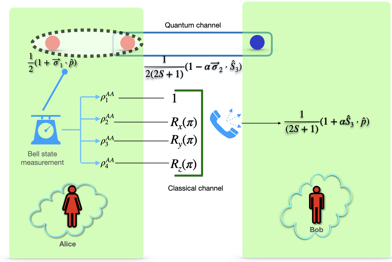
Let $\rho_{1}^{A}=\frac{1}{2}(\mathbb{1}+\vec{\sigma}_{1}\cdot\vec{p})$ be the unknown qubit with Alice whose equivalent is to be remotely prepared. The superscripts of a state indicate the parties having or sharing the state, e.g., $\rho^{AB}$ represents a bipartite state shared between Alice and Bob. The protocol is as follows:

1. 1.

   Alice has two qubits:

   1. (a)

      a qubit, unknown to her, whose information is to be transferred remotely,

   2. (b)

      the qubit of $\rho^{AB}(\alpha)^{1/2\otimes S}$, which has a shared correlation with the qudit at Bob.

   Thus, the combined state of Alice and Bob is given as

   $${\rho}^{A}_{1}\otimes\rho^{AB}(\alpha)^{1/2\otimes S}=\frac{1}{2^{2}(2S+1)}(\mathbb{1}+\vec{\sigma}_{1}\cdot\vec{p})\otimes(\mathbb{1}-\alpha\vec{\sigma}_{2}\cdot\hat{S}_{3}).$$

   (20)

2. 2.

   Alice performs a measurement in the Bell basis on her two qubits. She gets one of the four Bell states given below, with equal probability of $1/4$:

   		$\displaystyle\rho^{AA}_{1}=\dfrac{1}{4}\big(\mathbb{1}-\vec{\sigma}_{1}\cdot\vec{\sigma}_{2}\big);\penalty\$	$\displaystyle\rho^{AA}_{2}=\dfrac{1}{4}\big(\mathbb{1}-\sigma_{1x}\sigma_{2x}+\sigma_{1y}\sigma_{2y}+\sigma_{1z}\sigma_{2z}\big),$
   		$\displaystyle\rho^{AA}_{3}=\dfrac{1}{4}\big(\mathbb{1}+\sigma_{1x}\sigma_{2x}-\sigma_{1y}\sigma_{2y}+\sigma_{1z}\sigma_{2z}\big);\penalty\$	$\displaystyle\rho^{AA}_{4}=\dfrac{1}{4}\big(\mathbb{1}+\sigma_{1x}\sigma_{2x}+\sigma_{1y}\sigma_{2y}-\sigma_{1z}\sigma_{2z}\big).$

3. 3.

   She sends the information about her measurement outcome through a classical channel to Bob. Depending upon the information received, Bob performs a corresponding rotation on his state to retrieve the equivalent state of the qubit.

4. 4.

   If Alice obtains $\rho_{1}^{AA},\rho_{2}^{AA},\rho_{3}^{AA},\rho_{4}^{AA}$, the transformations that Bob has to apply on his qudit are $\mathbb{1},R_{x}(\pi),R_{y}(\pi),R_{z}(\pi)$ respectively. The symbols $R_{x}(\pi),R_{y}(\pi),R_{z}(\pi)$ represent Wigner rotation matrices of spin–$S$ about $x,y,$ and $z$ axes through an angle $\pi$. After performing the rotations, the state at Bob is $\tilde{\rho}^{B}_{1}(\alpha)\equiv\frac{1}{2S+1}(\mathbb{1}+\alpha\hat{S_{3}}\cdot\hat{p})$. Different transformations to be applied by Bob depending on the measurement outcomes of Alice are summarised in the table (1).

Thus, following the procedure, the spin–$S$ equivalent state of an unknown qubit is prepared at Bob’s end. The calculations for all the four possibilities (in which Alice gets $\rho_{1}^{AA},\cdots,\rho^{AA}_{4}$) are shown below.

In this section, we lay down a protocol for remote transfer of information of a known qubit to a qudit. The quantum channel $\rho^{AB}(\alpha)$, as before, is the $2\times(2S+1)$ dimensional separable equivalent of $2\times 2$– entangled Werner state

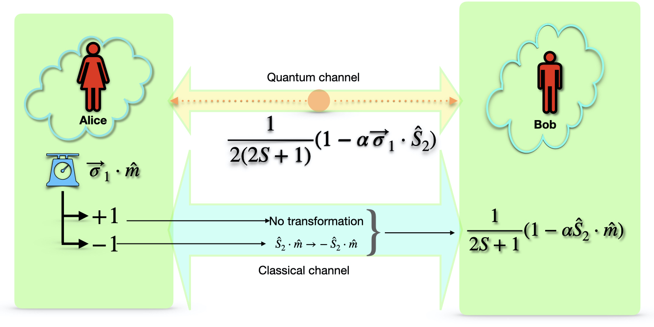
Let us assume Alice wants to transfer the information of her qubit $\frac{1}{2}(\mathbb{1}-\vec{\sigma_{1}}\cdot\hat{m})$ to Bob’s qudit. The steps to be performed by Alice are as follows:

1. 1.

   Alice measures $\vec{\sigma}_{1}\cdot\hat{m}$ on her qubit. She obtains either $+1$ or $-1$ with equal probability of $1/2$.

2. 2.

   If she obtains $\pm 1$ as the measurement outcome, her subsystem collapses to the state $\pi_{\hat{m}}^{\pm}=\dfrac{1}{2}(\mathbb{1}\pm\vec{\sigma}_{1}\cdot\hat{m})$. The normalised post-measurement state of Bob’s subsystem is

   $\displaystyle\rho^{B}_{pm}=\frac{1}{2S+1}\big\{\mathbb{1}\mp\alpha\hat{S}_{2}\cdot\hat{m}\big\}.$

   (27)

3. 3.

   If Alice obtains $+1$, she sends a classical message to Bob to do no transformation on his state. If Alice gets $-1$, she asks Bob to apply a rotation of $\pi$ about an axis perpendicular to $\hat{m}$ (such that $\hat{S}_{2}\cdot\hat{m}\rightarrow-\hat{S}_{2}\cdot\hat{m}$). This is because the state $\frac{1}{(2S+1)}\big\{\mathbb{1}+\alpha\hat{S}_{2}\cdot\hat{m}\big\}$ can be changed to $\frac{1}{(2S+1)}\big\{\mathbb{1}-\alpha\hat{S}_{2}\cdot\hat{m}\big\}$ by this transformation. Thus, Alice can prepare the requisite state at Bob’s end by sending one bit of classical information.

The pictorial representation of the proposed protocol is shown in Fig. 3.

In this section, we propose a protocol for the transfer of information of vector polarisation in the spin operator basis of an unknown qudit to a remotely located qudit. As before, the $1/2\otimes S$ separable equivalent of the $1/2\otimes 1/2$ Werner state,

acts as a quantum channel in this protocol. The steps of the protocol are as follows:

1. 1.

   Let $\rho^{A}=\frac{1}{2S+1}(\mathbb{1}+\hat{S}_{1}\cdot\vec{p})$ be the $(2S+1)$–dimensional state whose information is to be transferred by Alice. Thus, Alice has two subsystems; (i) the unknown state whose information she wants to transfer to a remote qudit, (ii) the other qubit which has shared correlation with Bob’s qudit.

2. 2.

   Alice performs a measurement of $\hat{S}_{1}\cdot\vec{\sigma}_{2}$, which is a dichotomic observable having eigenvalues $+1$ and $-\frac{S+1}{S}$. The two eigenvalues are degenerate with respective degeneracies of $2(S+1)$ and $2S$ respectively. The corresponding eigenprojections are

   	$\displaystyle\Pi_{1}=\frac{S+1}{2S+1}\Big(\mathbb{1}+\frac{S}{S+1}\hat{S}_{1}\cdot\vec{\sigma}_{2}\Big),$
   	$\displaystyle\Pi_{2}=\frac{S}{2S+1}(\mathbb{1}-\hat{S_{1}}\cdot\vec{\sigma}_{2}).$		(35)

3. 3.

   Upon measurement of $\Pi_{1}$ and $\Pi_{2}$ by Alice, the respective post-measurement states at Bob are $\frac{1}{2S+1}\Big(\mathbb{1}-\frac{\alpha}{3}\hat{S}_{3}\cdot\vec{p}\Big)$ and $\frac{1}{2S+1}\Big(\mathbb{1}+\alpha\frac{S+1}{3S}\hat{S}_{3}\cdot\vec{p}\Big)$ with probabilities $\frac{S+1}{2S+1}$ and $\frac{S}{2S+1}$ respectively.

4. 4.

   After performing the measurement, Alice sends Bob information about her measurement result. If Alice obtains $+1$, the direction of polarisation vector of Bob’s qudit is opposite to that of Alice’s qudit. On the other hand, if Alice gets $-\frac{S+1}{S}$, the direction of polarisation vector of Bob’s qudit is the same as that of Alice’s qudit. Since Bob has the knowledge of the channel, he knows that in both the cases, the polarisation vector of the qudit obtained by him has shrunk by a factor of approximately $\frac{1}{3}$ as compared to the qudit at Alice.

5. 5.

   As Bob is interested in the information encoded in the polarization vector, he needs to measure equivalent observables, proposed in Bharath14; given as $\frac{3S}{S+1}\hat{S}\cdot\hat{m}$, where $\hat{m}\in\{\hat{x},\hat{y},\hat{z}\}$. As explained in the protocol, the magnitude of the polarization vector is diminished by a constant factor $\frac{1}{3}$ which is a characteristic of the channel used. Therefore, it can be compensated by an extra factor of $3$ in the observable to be measured for retrieval of information (as explained in (2.2.1) for the example of magnetic moment). Thus, Bob can retrieve full information about the polarization vector by measurement of appropriate observables.

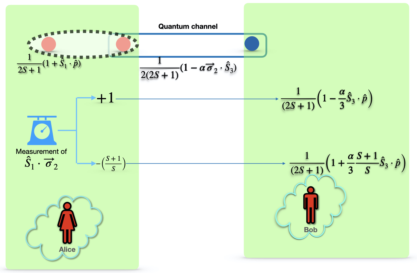
The calculations for this are shown in appendix (B). The protocol is schematically shown in Fig. 6.

The advantage of this protocol is that in place of an entangled state, a mixed separable (but discordant) state acts as a quantum channel. The above protocol can be used to send only those qudit states which have only non-zero vector polarization. However, this restriction can be relaxed if one uses the equivalent of higher dimensional entangled states.

Swapping of quantum correlations has been an interesting area of study, with the celebrated protocol proposed in Zukowski93 for entanglement swapping. Remote transfer of Gaussian quantum discord and swapping of quantum correlations between two-qubit Werner states have been earlier studied in Ma14 and Xie15 respectively.

In this section, we describe a protocol for swapping of quantum discord from $\frac{1}{2}\otimes S$ systems to $S\otimes S$ systems. For this, let there be four parties named as Alice, Bob, Charlie and David. Let the states shared between the pairs (Alice, Bob) and (Charlie, David) be $\frac{1}{2(2S+1)}(\mathbb{1}-\alpha\vec{\sigma}_{1}\cdot\hat{S}_{2})$ and $\frac{1}{2(2S+1)}(\mathbb{1}-\beta\hat{S}_{3}\cdot\vec{\sigma}_{4})$ respectively. These states are separable equivalents of $\frac{1}{4}(\mathbb{1}-\alpha\vec{\sigma}_{1}\cdot\vec{\sigma}_{2})$ and $\frac{1}{4}(\mathbb{1}-\beta\vec{\sigma}_{3}\cdot\vec{\sigma}_{4})$ respectively. Note that the minimum value of $S$ gets fixed according to the values of $\alpha$ or $\beta$, as discussed in the section (2.3). Obviously, the states shared between the pairs (Alice, Bob) and (Charlie, David) are discordant states. There is no correlation between the pairs (Alice, David) and (Bob, Charlie). In this protocol, we show that quantum discord can be generated between Bob and Charlie, which are a-priori uncorrelated, by appropriate measurements.

The combined state of all the four-parties is as follows:

If a measurement in the Bell basis is performed by Alice and David, the resultant state of Bob and Charlie will be discordant. For example, if a measurement of the singlet state is performed on the first and the fourth party, i.e., $\dfrac{1}{4}\{\mathbb{1}-\vec{\sigma}_{1}\cdot\vec{\sigma}_{4}\}$ is measured, then

Similar calculations for the other three Bell states are shown in Appendix(C). The transformation to be applied by Bob corresponding to different measurements performed by Alice and David are shown in table (2).

Thus, by having two lower-dimensional discordant states $\frac{1}{2(2S+1)}(\mathbb{1}-\alpha\vec{\sigma}_{1}\cdot\hat{S}_{2})$ and $\frac{1}{2(2S+1)}(\mathbb{1}-\beta\hat{S}_{3}\cdot\vec{\sigma}_{4})$, a higher dimensional discordant state $\frac{1}{(2S+1)^{2}}(\mathbb{1}-\alpha\beta\hat{S}_{2}\cdot\hat{S}_{3})$ can be produced. The schematic representation of the protocol is given in Fig. 7.

The protocols proposed in sections (3.1) and (3.4) involve Bell state measurements. Fortunately, due to their vital role, Bell state measurements have been studied extensively Lutkenhaus99; Ghosh01; Calsamiglia02; Cao20; Fan21. These studies would play a crucial role in the experimental implementation of the protocols.

At this stage, it is worthwhile to consider the future prospects of quantum communication with equivalent states and possible advantages that they would afford. Firstly, generalisations of our protocols to higher dimensional and multi-party systems constitute an interesting area of study. In fact, our protocols can be immediately generalised to remote transfer of information encoded in qutrits to remote qudits. This would require employment of the separable equivalents of $SU(2)$–invariant $3\times N$ level systems, as presented in Adhikary16. Secondly, these protocols provide a motivation for the identification of higher dimensional separable equivalent states of multi-party entangled systems, which is an interesting theoretical problem by itself. Those equivalent states can be employed for distribution of quantum information over a quantum network. In fact, a number of possibilities emerge when we seek to determine $k$–separable higher dimensional equivalent states of an $N$–party lower dimensional fully entangled state. The condition, $k=N$, implies a fully separable state, whereas $k=1,\cdots,(N-1)$ represent partially entangled states, which are equivalent to a fully entangled state in lower dimensions. Finally, this work shows the existence of quantum communication protocols in which we can dispense with entanglement.

References

- (1) J. S. Bell. On the einstein podolsky rosen paradox. Physics, 1:195, 1964.
- (2) Ryszard Horodecki, Paweł Horodecki, Michał Horodecki, and Karol Horodecki. Quantum entanglement. Rev. Mod. Phys., 81:865–942, Jun 2009.
- (3) H. M. Wiseman, S. J. Jones, and A. C. Doherty. Steering, entanglement, nonlocality, and the einstein-podolsky-rosen paradox. Phys. Rev. Lett., 98:140402, Apr 2007.
- (4) Harold Ollivier and Wojciech H. Zurek. Quantum discord: A measure of the quantumness of correlations. Phys. Rev. Lett., 88:017901, Dec 2001.
- (5) Charles H. Bennett, Gilles Brassard, Claude Crépeau, Richard Jozsa, Asher Peres, and William K. Wootters. Teleporting an unknown quantum state via dual classical and einstein-podolsky-rosen channels. Phys. Rev. Lett., 70:1895–1899, Mar 1993.
- (6) Charles H. Bennett and Stephen J. Wiesner. Communication via one- and two-particle operators on einstein-podolsky-rosen states. Phys. Rev. Lett., 69:2881–2884, Nov 1992.
- (7) Charles H. Bennett, David P. DiVincenzo, Peter W. Shor, John A. Smolin, Barbara M. Terhal, and William K. Wootters. Remote state preparation. Phys. Rev. Lett., 87:077902, Jul 2001.
- (8) Umesh Vazirani and Thomas Vidick. Fully device-independent quantum key distribution. Phys. Rev. Lett., 113:140501, Sep 2014.
- (9) M. Żukowski, A. Zeilinger, M. A. Horne, and A. K. Ekert. “event-ready-detectors” bell experiment via entanglement swapping. Phys. Rev. Lett., 71:4287–4290, Dec 1993.
- (10) Sandu Popescu. Bell’s inequalities versus teleportation: What is nonlocality? Phys. Rev. Lett., 72:797–799, Feb 1994.
- (11) Yun-Feng Huang, Bi-Heng Liu, Liang Peng, Yu-Hu Li, Li Li, Chuan-Feng Li, and Guang-Can Guo. Experimental generation of an eight-photon greenberger–horne–zeilinger state. Nature communications, 2(1):1–6, 2011.
- (12) Thomas Monz, Philipp Schindler, Julio T. Barreiro, Michael Chwalla, Daniel Nigg, William A. Coish, Maximilian Harlander, Wolfgang Hänsel, Markus Hennrich, and Rainer Blatt. 14-qubit entanglement: Creation and coherence. Phys. Rev. Lett., 106:130506, Mar 2011.
- (13) Xing-Can Yao, Tian-Xiong Wang, Ping Xu, He Lu, Ge-Sheng Pan, Xiao-Hui Bao, Cheng-Zhi Peng, Chao-Yang Lu, Yu-Ao Chen, and Jian-Wei Pan. Observation of eight-photon entanglement. Nature photonics, 6(4):225–228, 2012.
- (14) Borivoje Dakić, Yannick Ole Lipp, Xiaosong Ma, Martin Ringbauer, Sebastian Kropatschek, Stefanie Barz, Tomasz Paterek, Vlatko Vedral, Anton Zeilinger, Časlav Brukner, et al. Quantum discord as resource for remote state preparation. Nature Physics, 8(9):666–670, 2012.
- (15) Vaibhav Madhok and Animesh Datta. Quantum discord as a resource in quantum communication. International Journal of Modern Physics B, 27(01n03):1345041, 2013.
- (16) Alejandro Fonseca. High-dimensional quantum teleportation under noisy environments. Phys. Rev. A, 100:062311, Dec 2019.
- (17) Benjamin Perez-Garcia, Melanie McLaren, Sandeep K Goyal, Raul I Hernandez-Aranda, Andrew Forbes, and Thomas Konrad. Quantum computation with classical light: Implementation of the deutsch–jozsa algorithm. Physics Letters A, 380(22-23):1925–1931, 2016.
- (18) Benjamin Perez-Garcia, Raul I. Hernandez-Aranda, Andrew Forbes, and Thomas Konrad. The first iteration of grover’s algorithm using classical light with orbital angular momentum. Journal of Modern Optics, 65(16):1942–1948, 2018.
- (19) Robert J. C. Spreeuw. Classical wave-optics analogy of quantum-information processing. Phys. Rev. A, 63:062302, May 2001.
- (20) Sandeep K. Goyal, Filippus S. Roux, Andrew Forbes, and Thomas Konrad. Implementing quantum walks using orbital angular momentum of classical light. Phys. Rev. Lett., 110:263602, Jun 2013.
- (21) H. M. Bharath and V. Ravishankar. Classical simulation of entangled states. Phys. Rev. A, 89:062110, Jun 2014.
- (22) Soumik Adhikary, Ipsit Kumar Panda, and V. Ravishankar. Super-quantum states in su(2) invariant level systems. Annals of Physics, pages –, 2016.
- (23) Gabriel Molina-Terriza, Juan P Torres, and Lluis Torner. Twisted photons. Nature physics, 3(5):305–310, 2007.
- (24) Manuel Erhard, Robert Fickler, Mario Krenn, and Anton Zeilinger. Twisted photons: new quantum perspectives in high dimensions. Light: Science & Applications, 7(3):17146–17146, 2018.
- (25) J M Radcliffe. Some properties of coherent spin states. Journal of Physics A: General Physics, 4(3):313–323, may 1971.
- (26) R. F. Werner. Quantum states with einstein-podolsky-rosen correlations admitting a hidden-variable model. Physical Review A, 40(8):4277, October 1989.
- (27) Michael A Nielsen and Isaac L Chuang. Quantum information and quantum computation. Cambridge: Cambridge University Press, 2(8):23, 2000.
- (28) V. Bužek and M. Hillery. Quantum copying: Beyond the no-cloning theorem. Phys. Rev. A, 54:1844–1852, Sep 1996.
- (29) Matthias Bock, Andreas Lenhard, Christopher Chunnilall, and Christoph Becher. Highly efficient heralded single-photon source for telecom wavelengths based on a ppln waveguide. Optics express, 24(21):23992–24001, 2016.
- (30) Yijie Shen, Xuejiao Wang, Zhenwei Xie, Changjun Min, Xing Fu, Qiang Liu, Mali Gong, and Xiaocong Yuan. Optical vortices 30 years on: Oam manipulation from topological charge to multiple singularities. Light: Science & Applications, 8(1):1–29, 2019.
- (31) Miles J Padgett. Orbital angular momentum 25 years on. Optics express, 25(10):11265–11274, 2017.
- (32) Lingyu Ma and Xiaolong Su. Remote transfer of gaussian quantum discord. Optics express, 22(13):15894–15903, 2014.
- (33) Chuanmei Xie, Yimin Liu, Hang Xing, Jianlan Chen, and Zhanjun Zhang. Quantum correlation swapping. Quantum Information Processing, 14(2):653–679, 2015.
- (34) N. Lütkenhaus, J. Calsamiglia, and K.-A. Suominen. Bell measurements for teleportation. Phys. Rev. A, 59:3295–3300, May 1999.
- (35) Sibasish Ghosh, Guruprasad Kar, Anirban Roy, Aditi Sen(De), and Ujjwal Sen. Distinguishability of bell states. Phys. Rev. Lett., 87:277902, Dec 2001.
- (36) John Calsamiglia. Generalized measurements by linear elements. Phys. Rev. A, 65:030301, Feb 2002.
- (37) Cong Cao, Li Zhang, Yu-Hong Han, Pan-Pan Yin, Ling Fan, Yu-Wen Duan, and Ru Zhang. Complete and faithful hyperentangled-bell-state analysis of photon systems using a failure-heralded and fidelity-robust quantum gate. Optics express, 28(3):2857–2872, 2020.
- (38) Ling Fan and Cong Cao. Deterministic cnot gate and complete bell-state analyzer on quantum-dot-confined electron spins based on faithful quantum nondemolition parity detection. JOSA B, 38(5):1593–1603, 2021.