1Introduction

Gravitino Dark matter, Non Thermal Leptogenesis and Low reheating temperature in No-scale Higgs Inflation.

Waqas Ahmed^a ¹¹ 1 E-mail: waqasmit@nankai.edu.cn , waqasmit@hbpu.edu.cn, Athanasios Karozas^b ²² 2 E-mail: akarozas@uoi.gr and George K. Leontaris^b ³³ 3 E-mail: leonta@uoi.gr

^a School of Mathematics and Physics, Hubei Polytechnic University,

No. 16 North Road, Guilin, Huangshi, Hubei, China

^b Physics Department, Theory Division, University of Ioannina,

GR-45110 Ioannina, Greece

We revisit Higgs inflation in the framework of a minimal extension of the Standard Model gauge symmetry by a $U(1)_{B-L}$ factor. Various aspects are taken into account with particular focus on the role of the supersymmetry breaking (SUSY) scale and the cosmological constraints associated with the gravitino. The scalar potential of the model is considered in the context of no-scale supergravity consisting of the F-part constructed from the Kähler function, the D-terms and soft SUSY contributions. We investigate several limiting cases and by varying the SUSY scale from a few TeV up to intermediate energies, for a spectral index around $n_{s}\sim 0.9655$ and reheating temperature $T_{r}\leq 10^{9}$ GeV we find that the value of the tensor-to-scalar ratio ranges from $r\approx 10^{-3}$ to $10^{-2}$ . Furthermore it is shown that for certain regions of the parameter space the gravitino can live sufficiently long and as such is a potential candidate for a dark matter component. In general, the inflationary scenario is naturally implemented and it is consistent with non-thermal leptogenesis whereas the dominant decay channel of the inflaton yields right-handed neutrinos. Other aspects of cosmology and particle physics phenomenology are briefly discussed. Finally, we investigate the case where the inflaton is initially relaxed in a false minimum and estimate its probability to decay to the true vacuum.

1 Introduction

The theory of cosmological inflation has indisputable advantages. Among other implications, it provides convincing answers to the flatness and horizon problems [1, 2, 3], and explains the origin of the large scale structure of the universe.

During the last few decades numerous scenarios have been proposed to formulate a detailed microscopic mechanism for a complete theory of inflation with successful predictions for all related observables. The Cosmic Microwave Background (CMB) observations, however, put rather tight constraints on many inflationary theories [4, 5]. Several models such as those with quartic and quadratic potentials fail to satisfy the bound on the tensor to scalar ratio, (which according to Planck 2018 results is $r<0.05$ at $95\%$ confidence level [5]), hence such models are ruled out. On the other side, one of the most successful inflationary models, which is in accordance with the Planck 2018 results, is the Starobinsky model [1] which predicts $n_{s}=1-\frac{2}{N_{0}}$ and $r=\frac{12}{N^{2}_{0}}\sim\left(0.002-0.004\right)$ , where $N_{0}$ represents the numbers of e-folds. The Starobinsky inflationary potential has been studied extensively in the literature within various contexts, while it was shown that this model can be derived in the context of no-scale supergravity (SUGRA) [6, 7, 8, 9, 10, 11, 12, 13]. The simplest version of the Starobinsky proposal is equivalent to an inflationary model in which the scalar field couples non-minimally to gravity. A natural choice for the inflaton field in Grand Unified Theories (GUTs) in the context of supergravity, is the Higgs field breaking the GUT symmetry [14, 15, 16, 17, 18]. Inflation with Standard Model (SM) like Higgs boson in the Minimal Supersymmetric Standard Model (MSSM) has also been proposed [10, 12, 19]. Also, in [20, 21] non-supersymmetric models with non-minimal Higgs inflation is discussed. Several other ideas including [22] chaotic, hybrid and hilltop inflation have been proposed and investigated in detail. Some of these scenarios can also be realized in a string theory framework where the role of the inflaton field is played by some modulus.

Hybrid Inflation in particular, is one of the most promising models of inflation, and can be naturally realized within the context of supergravity theories. This scenario is based on the inclusion of two scalar fields [23], with the first one realizing the slow-roll inflation and the second one, dubbed the “waterfall” field, triggering the end of inflationary epoch. While in the standard hybrid inflationary scenario [24, 25, 26] in the supersymmetric GUTs, the symmetry is broken at the end of inflation, in the case of shifted [27] and smooth inflation [28], the symmetry breaking occurs during inflation and thus, magnetic monopoles and other topological defects are inflated away.

On the side of particle physics, the experimental data collected at the Large Hadron Collider (LHC) so far, put strong constraints on the conventional SUSY scenarios with superpartner masses around the electroweak scale. The so far null SUSY experimental results have triggered significant interest in alternative SUSY scale scenarios, such as high-scale SUSY and split SUSY among others [29, 30]. Taking into account the possible connection between inflationary dynamics and SUSY scale phenomenology it will be interesting to study the effects among various SUSY scale scenarios with a successful model of inflation.

In this paper we study inflation in a supergravity context where a no-scale Kähler potential is assumed. We consider the framework of the SM gauge symmetry augmented by a $U(1)_{B-L}$ factor [31, 32, 33]. In this background, after employing the mechanism proposed in [34, 35] for dynamically generating a $\mu$ -term, we investigate the implementation of cosmic inflation and its interplay with the issues of SUSY scale, non-thermal leptogenesis and gravitino dark matter. We show that for TeV and Split SUSY scenarios the tensor-to-scalar ratio remains as low as $r\approx{\cal O}(10^{-3})$ , while for a High scale SUSY scenario $r$ receives higher values of the order $r\sim\mathcal{O}(10^{-2})$ with the spectral index fixed at its central value $n_{s}=0.9655$ and reheating temperature $T_{r}<5\times 10^{9}$ GeV. We also discuss the process of non-thermal leptogenesis and show that the dominant inflaton decay channel yields right handed neutrinos. For gravitino cosmology, we explore three possibilities: stable, unstable long-lived and unstable short-lived gravitino. For the various cases we investigate the reheating and cosmological gravitino constraints and we find a consistent inflationary scenario, that gives rather concrete predictions regarding supersymmetric dark matter and LHC phenomenology. We complete our analysis with an investigation of certain regions of the parameters which yield a potential containing a false minimum. We examine possible scenaria of quantum tunneling effects and compute the decay probability of such vacua to the true vacuum.

The layout of the paper is as follows. In Sec. 2 we describe the basic features of the model including the superfields, their charge assignments, and the superpotential constrained by a $U(1)$ R symmetry. The inflationary setup is described in Sec. 3. The numerical analysis is presented in Sec. 4 containing the prospects of observing primordial gravity waves and non-thermal leptogenesis. In sections 5 and 6 we discuss the gravitino cosmology and quantum tunneling. Our conclusions are summarized in Sec 7.

Superfields	Representations	Global Symmetries
	under $G_{B-L}$	$R$	$B$	$L$
Matter Fields
$e^{c}_{i}$	$({\bf 1,1},1,1)$	$1$	$0$	$-1$
$N^{c}_{i}$	$({\bf 1,1},0,1)$	$1$	$0$	$-1$
$L_{i}$	$({\bf 1,2},-1/2,-1)$	$1$	$0$	$1$
$u^{c}_{i}$	$({\bf 3,1},-2/3,-1/3)$	$1$	$-1/3$	$0$
$d^{c}_{i}$	$({\bf 3,1},1/3,-1/3)$	$1$	$-1/3$	$0$
$Q_{i}$	$({\bf\bar{3},2},1/6,1/3)$	$1$	$1/3$	$0$
Higgs Fields
$H_{d}$	$({\bf 1,2},-1/2,0)$	$0$	$0$	$0$
$H_{u}$	$({\bf 1,2},1/2,0)$	$0$	$0$	$0$
$S$	$({\bf 1,1},0,0)$	$2$	$0$	$0$
$\overline{H}$	$({\bf 1,1},0,2)$	$0$	$0$	$-2$
$H$	$({\bf 1,1},0,-2)$	$0$	$0$	$2$

Table 1: Superfield content of the model, the corresponding representations under the local gauge symmetry

U_{B-L}

and the properties with respect to the extra global symmetries.

2 Description of the Model

In this section we will present the basic features regarding the gauge symmetry and the spectrum of the effective model in which the inflationary scenario will be implemented. The gauge symmetry is the Standard Model gauge group extended by a $U_{B-L}$ abelian gauge symmetry

G_{B-L}=SU(3)_{C}\times{SU(2)_{L}}\times U(1)_{Y}\times{U(1)_{B-L}}~\cdot

(2.1)

The particle content of the model contains the MSSM matter and Higgs representations, three singlets accommodating the right-handed neutrinos $N_{i}^{c}$ , a neutral scalar singlet $S$ and a pair of Higgs singlets $H$ , $\overline{H}$ . These are listed in Table 1, where in addition to the transformation properties under (2.1), the ‘charges’ under the global symmetries $R,B,L$ also are shown.

When the $H$ , $\overline{H}$ singlet Higgs fields acquire vacuum expectation values (VEVs), they break the $U(1)_{B-L}$ symmetry and, at the same time, they provide Majorana masses to the right handed neutrinos. For the field content and the corresponding charge assignments given in Table 1, the renormalizable superpotential of the model is

\begin{split}W&=y_{u}{H_{u}}{q}{u}^{c}+y_{d}{H_{d}}{q}{d}^{c}+y_{e}{H_{d}}{L}{e}^{c}+y_{\nu}{H_{u}}{L}{N}^{c}\\ &+\kappa S\left(\overline{H}H-M^{2}\right)+\lambda SH_{u}H_{d}+\beta HN^{c}N^{c}\;.\end{split}

(2.2)

The first line contains the Yukawa sector providing Dirac masses to the up and down quarks, charged leptons and neutrinos. The corresponding Yukawa couplings are denoted with $y_{u}$ , $y_{d}$ , $y_{e}$ and $y_{\nu}$ and the family indices are generally suppressed for simplicity. The tree-level terms in the second line involve the extra fields beyond the MSSM spectrum. The first term describes the standard supersymmetric Hybrid Inflation model with $M$ being a GUT scale mass parameter and $\kappa$ a coupling constant coefficient. The second term, generates dynamically a $\mu$ -term for the model when the singlet scalar $S$ receives a non-zero VEV. The $H$ and $\overline{H}$ fields carry non-zero $B-L$ charges and their VEV’s spontaneously break the $U(1)_{B-L}$ symmetry. Furthermore, $H$ is responsible for generating a Majorana mass for the right-handed neutrinos through the last term in (2.2). By virtue of the extra global symmetries, the model is protected from dangerous proton decay operators and R-parity violating terms. For the same reason, bilinear terms of form $H_{u}H_{d}$ and $H\overline{H}$ are absent too. After this short description of the salient features of the model, in the next section we proceed with the inflationary dynamics.

3 Inflation potential

We will compute the effective scalar potential considering contributions from the F- and D-sector, as well as soft supersymmetry breaking terms. The superpotential terms relevant for inflation are

W\supset\kappa S\left(\overline{H}H-M^{2}\right)+\lambda SH_{u}H_{d}+\beta HN^{c}N^{c}\;.

(3.1)

We consider a no-scale structure Kähler potential which, after including contributions of the relevant fields in the present model, takes the form (from now on we set the reduced Planck mass to unity, $M_{Pl}=1$ ):

\displaystyle\begin{split}K&=-3\log\left[T+T^{\ast}-\frac{1}{3}\left(HH^{\ast}+\bar{H}\bar{H}^{\ast}+H_{u}H_{u}^{\ast}+H_{d}H_{d}^{\ast}+S^{\dagger}S+{N^{c}}^{\dagger}N^{c}\right)\right.\\ &\left.+\frac{\xi}{3}\left(H\bar{H}+H^{\ast}\bar{H}^{\ast}\right)+\frac{\zeta}{3}\left(H_{u}H_{d}+H_{u}^{\ast}H_{d}^{\ast}\right)\right],\end{split}

(3.2)

where $T$ , $T^{*}$ are Kähler moduli fields and $\xi$ , $\zeta$ are dimensionless parameters. For later convenience we define

\displaystyle\begin{split}\Delta&=\left[T+T^{\ast}-\frac{1}{3}\left(HH^{\ast}+\bar{H}\bar{H}^{\ast}+H_{u}H_{u}^{\ast}+H_{d}H_{d}^{\ast}+S^{\dagger}S+{N^{c}}^{\dagger}N^{c}\right)\right.\\ &\left.+\frac{\xi}{3}\left(H\bar{H}+H^{\ast}\bar{H}^{\ast}\right)+\frac{\zeta}{3}\left(H_{u}H_{d}+H_{u}^{\ast}H_{d}^{\ast}\right)\right]~,\end{split}

(3.3)

hence, equation (3.2) is simply written as $\text{K}=-3\log\Delta$ . Furthermore, we introduce the standard definition of the Kähler function

G=K+\log|W|^{2}\equiv K+\log W+\log W^{*}.

Then, the F-term potential is given by

\displaystyle V_{F}=e^{G}\left(G_{i}G_{ij^{*}}^{-1}G_{j^{*}}-3\right),

(3.4)

where $G_{i}(G_{j^{*}})$ are the derivatives with respect to the various scalar fields appearing (3.2). Using the above ingredients the F-term potential (3.4) takes the form

\displaystyle\begin{split}V_{F}&=\frac{1}{\Delta^{2}}\left[\kappa^{2}\left(M^{2}-H\overline{H}\right)^{2}+\kappa^{2}S^{2}\left(H^{2}+\overline{H}^{2}\right)+\lambda^{2}\left(H_{u}^{2}H_{d}^{2}+S^{2}H_{u}^{2}+S^{2}H_{d}^{2}\right)\right.\\ &+\left.{N^{c}}^{2}\left(\beta^{2}{N^{c}}^{2}+4\beta^{2}\overline{H}^{2}+2\beta\kappa SH\right)-2\kappa\lambda H\overline{H}H_{u}H_{d}-2\kappa\lambda M^{2}H_{u}H_{d}\right.].\end{split}

(3.5)

When the Higgs doublets $H_{u},H_{d},$ and the various singlet fields $H,\bar{H},S,N^{c},$ are eliminated and only the Kähler moduli are present, the no-scale structure of the Kähler potential implies that the effective F-term potential vanishes identically, $V_{F}\equiv 0$ . We first explore inflation along the $H$ direction, starting with the supersymmetric global minima of the potential. It can be observed that the global minimum of the above potential lies at

S^{0}=H_{u}^{0}=H_{d}^{0}={N^{c}}^{0}=0~,

(3.6)

and

\begin{split}H^{0}=0,\quad H^{0}=\pm M,\end{split}

(3.7)

where $H^{0}=0$ corresponds to an extremum and $H^{0}=\pm M$ to local minima.

Next, we turn to the D-term potential. For the fields carrying ${B-L}$ quantum numbers, (shown in Table 1 and denoted collectively here with $\phi_{i}$ ), the D-term potential is,

\displaystyle V_{D}=\frac{1}{2}D^{p}_{a}D^{p}_{a}~,

(3.8)

where

D_{a}^{p}=-g_{a}K_{,\phi_{i}}\left[t_{a}^{p}\right]_{i}^{j}\phi_{j}

for $SU(N)$ groups and $D^{a}$ is defined as,

D_{a}^{p}=-g_{a}K_{,\phi_{i}}\left[t_{a}^{p}\right]_{i}^{j}\phi_{j}-g_{a}q_{i}\varsigma~,

in the presence of $U(1)$ symmetries. Here $q_{i}$ is the charge under $U(1)$ , the symbol $\varsigma$ stands for the Fayet-Iliopoulos coupling constant and $K_{,\phi_{i}}\equiv dK/d\phi_{i}$ . The $t_{a}^{p}$ are the generators of the corresponding group $G$ and $p=1,...,{\rm dim}(G)$ . The D-term potential can be written as,

\displaystyle\begin{split}V_{D}&=\frac{g_{b}^{2}}{2\Delta^{2}}\left[\phi_{i}^{\ast}\left(t_{b}^{p}\right)_{i}^{j}\phi_{j}-\zeta\bar{\phi}\left(t_{b}^{p}\right)_{i}^{j}\phi_{j}\right]^{2}+\frac{g_{B-L}^{2}}{2\Delta^{2}}\left[\phi_{i}^{\ast}\left(t_{B-L}^{p}\right)_{i}^{j}\phi_{j}-\xi\bar{\phi}\left(t_{B-L}^{p}\right)_{i}^{j}\phi_{j}-q_{i}\varsigma\right]^{2}~,\end{split}

(3.9)

where $g_{b}\,(b=1,2,3)$ and $g_{B-L}$ correspond to the $SU(3)_{c}$ , $SU(2)_{L}$ , $U(1)_{Y}$ and $U(1)_{B-L}$ gauge couplings respectively. For our purposes, it suffices to work along $D$ -flat directions where the D-term potential $V_{D}$ vanishes. Restricting to the scalar fields, we first observe that they transform trivially under $SU(3)_{c}$ , thus the corresponding D-term is zero. The other three contributions are

\displaystyle\begin{split}V_{D}&=\frac{g_{1}^{2}}{2\Delta^{2}}\left[\frac{1}{2}\mid H_{u}\mid^{2}-\frac{1}{2}\mid H_{d}\mid^{2}-\zeta\left(\frac{1}{2}\bar{H_{d}}H_{u}-\frac{1}{2}\bar{H_{u}}H_{d}\right)\right]\\ &+\frac{g_{2}^{8}}{2\Delta^{2}}\left[H_{u}^{\ast}\sigma^{p}H_{u}+H_{d}^{\ast}\sigma^{p}H_{d}-\zeta\left(\bar{H_{d}}\sigma^{p}H_{u}+\bar{H_{u}}\sigma^{p}H_{d}\right)\right]^{2}\\ &+\frac{g_{B-L}^{2}}{2\Delta^{2}}\left[2\mid\bar{H}\mid^{2}-2\mid H\mid^{2}-\xi\left(2H\bar{H}-2\bar{H}H\right)+\left(q_{H}+q_{\bar{H}}\right)\varsigma\right]^{2}~.\end{split}

(3.10)

Here $\sigma^{p},\,p=1,2,3$ are the $SU(2)_{L}$ generators (Pauli matrices) and $H_{u},H_{d}$ are the MSSM doublet Higgs fields which in component notation will be written as

\displaystyle\begin{split}H_{u}&=\begin{pmatrix}H_{u}^{+}\\ H_{u}^{0}\end{pmatrix},\quad H_{d}&=\begin{pmatrix}H_{d}^{0}\\ H_{d}^{-}\end{pmatrix}~.\end{split}

(3.11)

Using $SU(2)_{L}$ transformation, it is possible to rotate the Higgs boson fields into the neutral directions $H_{u}^{0}$ and $H_{d}^{0}$ . A D-flat direction can be achieved with $H_{u}^{0}=H_{d}^{0}$ and $\bar{H}=H$ [36]. Finally, we may also include contributions from explicit soft SUSY-breaking terms of the form

\displaystyle\begin{split}V_{soft}=m^{2}\mid\phi_{i}\mid^{2}+\left(\kappa A_{\kappa}SH\bar{H}+\lambda A_{\mu}SH_{u}H_{d}+\beta A_{N^{c}}\bar{H}N^{c}N^{c}-a_{s}S\kappa M^{2}+h.c\right),\end{split}

(3.12)

where $A_{\kappa}=A_{\mu}=A_{N^{c}}$ are the complex coefficients of the trilinear soft-SUSY-breaking terms. Along the inflationary trajectory, $S$ is zero, so the corresponding trilinear terms do not contribute. Then, for $S=0$ the total effective potential $V(\varphi)=V_{F}+V_{D}+V_{soft}$ is

\displaystyle\begin{split}V(\varphi)&=\frac{9\kappa^{2}\left(M^{2}-H^{2}\right)^{2}}{\left(3(T+T^{\ast})-2(1-\xi)H^{2}\right)^{2}}+2m^{2}H^{2}.\end{split}

(3.13)

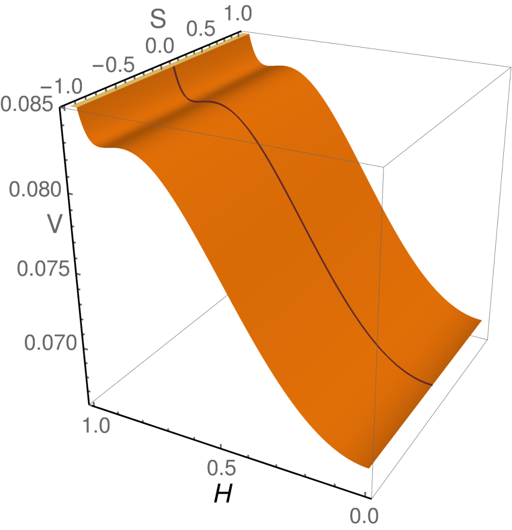
The shape of the effective potential is presented in Fig. 1. The left panel represents the potential as a function of $H$ and $S$ with the black curve corresponding to the $S=0$ direction. The right panel shows the potential as a function of $H$ for various values of $\xi$ and $S=0$ . Along the inflationary trajectory the vacuum energy density is non-zero. The non-zero field value during inflation also breaks $U(1)_{B-L}$ and the symmetry reduces down to SM. Since the gauge symmetry is broken during inflation, monopoles and cosmic strings are inflated away.

We define the inflaton field as ${\varphi}=2H$ and the modulus complex fields as $T=\left(u+i\,v\right)$ , hence $T+T^{\ast}=2u$ . Then the potential along the inflationary track is:

V\left(\varphi\right)=\frac{\kappa^{2}\left(M^{2}-\frac{\varphi^{2}}{4}\right)^{2}}{\left(2u-\left(\frac{1-\xi}{6}\right)\varphi^{2}\right)^{2}}+\frac{m^{2}}{2}\varphi^{2}=\frac{V_{0}\left(1-\frac{\varphi^{2}}{4M^{2}}\right)^{2}}{\left(2u-\left(\frac{1-\xi}{6}\right)\varphi^{2}\right)^{2}}+\frac{m^{2}}{2}\varphi^{2}\;,

(3.14)

Refer to caption — Figure 1: In the left panel we show the shape of the potential in 3-dimensions as a function of S and H. In the right panel we show the shape of the potential along the $H$ direction for different values of $\xi$ . In both plots we have fixed the other parameters as: $M=1$ , $m=0.2$ , $\kappa=0.26$ and $T=T^{\ast}=\frac{1}{2}$ .

where $V_{0}=\kappa^{2}M^{4}$ . However, the inflaton field $\varphi$ is not canonically normalized since its kinetic energy terms take the form,

\begin{split}\mathcal{L}\left(\varphi\right)=\frac{2u-\frac{\varphi^{2}}{6}\xi\left(1-\xi\right)}{2\left(2u-\frac{1}{6}\left(1-\xi\right)\varphi^{2}\right)^{2}}\left(\partial\varphi\right)^{2}-V({\varphi}).\end{split}

(3.15)

We introduce a canonically normalized field $\chi$ satisfying

\begin{split}\left(\frac{d\chi}{d\varphi}\right)^{2}=\frac{2u-\frac{\varphi^{2}}{6}\xi\left(1-\xi\right)}{\left(2u-\frac{1}{6}\left(1-\xi\right)\varphi^{2}\right)^{2}}.\end{split}

(3.16)

Integrating (while choosing $u=1/2$ ) we obtain the canonically normalized field $\chi$ as a function of $\varphi$ ,

\chi=\sqrt{6}\tanh^{-1}\left(\frac{\left(1-\xi\right)\varphi}{\sqrt{6\left(1-\frac{\xi\left(1-\xi\right)\varphi^{2}}{6}\right)}}\right)-\sqrt{\frac{6\xi}{1-\xi}}\sinh^{-1}\left(\sqrt{\xi\left(\frac{1-\xi}{6}\right)}\varphi\right).

(3.17)

3.1 The $\mu$ problem and a non-zero VEV for the $S$ field

In section 2, we have discussed the basic features of the model under consideration and introduced an $R$ symmetry to constrain the superpotential. In the present section we discuss the appearance of new contributions including those coming from supersymmetry breaking effects.

The supersymmetric Higgs mass parameter $\mu$ (associated with the so called $\mu$ problem [37]) can be generated when the $S$ field acquires a non-zero VEV not much higher than the electroweak scale. Contributions from the soft SUSY breaking terms, although negligible during inflation, may generate the required non-zero VEV, $\langle S\rangle\neq 0$ [34].

Furthermore, in principle, we can include a constant term $W_{0}$ in the superpotential (2.2) which gives rise to a gravitino mass [38]-[40] through the formula $m_{3/2}=e^{K/2}\langle W_{0}\rangle$ . The magnitude of the constant $W_{0}$ is model dependent and its presence in the superpotential has important implications on the dynamics of the effective theory. In the present model, however, $W_{0}$ violates the R-symmetry of the superpotential (2.2) which has been imposed in order to ensure linearity on $S$ and thereby the gravitino cannot acquire a mass whithin this context. Nevertheless, an alternative way to generate a non-zero $m_{3/2}$ that is rather appropriate here, is the mechanism described in [34] (see also [41]). This relies on the soft SUSY breaking superpotential terms mentioned above which shift the VEV of the field $S$ to a non-zero value $\langle S\rangle\neq 0$ . This is sufficient to solve the $\mu$ -problem and -at the same time- generate a non-zero mass for the gravitino.

Next, we focus on the scalar potential. Inserting the values $H^{0}=\pm M,N^{0}=0$ and $H_{u}^{0}=H_{d}^{0}=0$ the total potential takes the form,

V_{t}(S)=\frac{2\kappa^{2}M^{2}S^{2}}{\left(2u-\frac{2M^{2}(1-\xi)+S^{2}}{3}\right)}+m_{S}^{2}S^{2}+\kappa A_{\kappa}M^{2}S-a_{S}\kappa M^{2}+h.c.

(3.18)

Assuming $S\ll 1$ , we may expand the first term of (3.18) in powers of $S$ . Neglecting terms higher than $S^{2}$ in the expansion, the potential can be expressed in terms of the gravitino mass $m_{3/2}$ as follows,

V_{t}(S)=\frac{2\kappa^{2}M^{2}S^{2}}{\left(2u-\frac{2M^{2}(1-\xi)}{3}\right)^{2}}+m_{S}^{2}S^{2}+2b\kappa m_{3/2}M^{2}S~,

(3.19)

where we used $\mid a_{s}\mid+\mid A_{\kappa}\mid=2bm_{3/2}$ while the $m_{S}^{2}$ term has been neglected since $m_{S}^{2}\ll M^{2}$ . Minimisation of the potential now gives,

\sigma\equiv\langle S\rangle=-\frac{bm_{3/2}}{2\kappa}\left(2u-\frac{2M^{2}(1-\xi)}{3}\right)^{2}~.

(3.20)

The second derivative with respect to $S$ :

\frac{d^{2}V_{t}}{dS^{2}}\mid_{\sigma}=\frac{4\kappa^{2}M^{2}}{\left(2u-\frac{2M^{2}(1-\xi)}{3}\right)^{2}}>0~,

(3.21)

is always positive, and the potential acquires a minimum for $\langle S\rangle\neq 0$ . Hence, the $\mu$ parameter now is dynamically generated as long as $S$ receives a non zero VEV,

\mu=\lambda\sigma=-\frac{\lambda bm_{3/2}}{2\kappa}\left(2u-\frac{2M^{2}(1-\xi)}{3u}\right)^{2}.

(3.22)

Finally, for $\langle S\rangle\neq 0$ the effective potential takes the following form,

\begin{split}V\left(\varphi\right)&=\frac{\kappa^{2}\left(M^{2}-\frac{\varphi^{2}}{4}\right)^{2}+\frac{\kappa^{2}\sigma^{2}\varphi^{2}}{2}}{\left(2u-\left(\frac{1-\xi}{6}\right)\varphi^{2}-\frac{\sigma^{2}}{3}\right)^{2}}+\frac{m^{2}}{2}\varphi^{2}-\frac{b^{2}M^{2}m_{3/2}^{2}}{2}\left(2u-\frac{2M^{2}(1-\xi)}{3}\right)^{2}\;.\end{split}

(3.23)

So the Lagrangian in this case reads as,

\begin{split}\mathcal{L}\left(\varphi\right)=\frac{2u-\frac{\varphi^{2}}{6}\xi\left(1-\xi\right)}{2\left(2u-\frac{1}{6}\left(1-\xi\right)\varphi^{2}-\frac{\sigma^{2}}{3}\right)^{2}}\left(\partial\varphi\right)^{2}-V({\varphi})~,\end{split}

(3.24)

and the canonically normalized field $\chi$ now satisfies the equation

\begin{split}\chi^{\prime}\equiv\left(\frac{d\chi}{d\varphi}\right)=\sqrt{\frac{2u-\frac{\varphi^{2}}{6}\xi\left(1-\xi\right)}{\left(2u-\frac{1}{6}\left(1-\xi\right)\varphi^{2}-\frac{\sigma^{2}}{3}\right)^{2}}}~\cdot\end{split}

(3.25)

We turn now to a numerical analysis and compute the various observables related to infation.

Figure 2: The plot on the top shows predictions for the tensor to scalar ratio

r

as a function of the coupling constant

\beta

for various values of the reheating temperature

T_{r}

. Each curve corresponds to a fixed value of

T_{r}

. For all the curves we fix the GUT scale at

M=2\times{10^{16}}

GeV, the spectral index

n_{s}=0.9655

(central value), the gravitino mass and the higgsino mass parameter at

m_{3/2}=\mu=1

TeV. The remaining figures on the lower panels show the ranges for the other parameters (

m

\lambda

\kappa

\xi

) involved in the analysis with respect to the (

\beta,r

)-plot.

4 Analysis

In this section we analyse the implications of the model and discuss its predictions regarding the various cosmological observables. We pay particular attention to leptogenesis, large $r$ solutions and gravitational waves. Before presenting numerical predictions we briefly review the basic results of the slow-roll assumption.

4.1 Slow-roll approximation

The inflationary slow-roll parameters are given by:

\epsilon=\dfrac{1}{2}\left(\frac{V^{\prime}\left(\varphi\right)}{V(\varphi)\chi^{\prime}\left(\varphi\right)}\right)^{2},\quad\quad\eta=\left(\frac{V^{\prime\prime}\left(\varphi\right)}{V(\varphi)\left(\chi^{\prime}\left(\varphi\right)\right)^{2}}-\frac{V^{\prime}\left(\varphi\right)\chi^{\prime\prime}\left(\varphi\right)}{V(\varphi)\left(\chi^{\prime}\left(\varphi\right)\right)^{3}}\right).

(4.1)

The third slow-roll parameter is,

s^{2}=\left(\frac{V^{\prime}\left(\varphi\right)}{V(\varphi)\chi^{\prime}\left(\varphi\right)}\right)\left(\frac{V^{\prime\prime\prime}\left(\varphi\right)}{V(\varphi)\left(\chi^{\prime}\left(\varphi\right)\right)^{3}}-3\frac{V^{\prime\prime}\left(\varphi\right)\chi^{\prime\prime}\left(\varphi\right)}{V(\varphi)\left(\chi^{\prime}\left(\varphi\right)\right)^{4}}+3\frac{V^{\prime}\left(\varphi\right)\left(\chi^{\prime\prime}\left(\varphi\right)\right)^{2}}{V(\varphi)\left(\chi^{\prime}\left(\varphi\right)\right)^{5}}-\frac{V^{\prime}\left(\varphi\right)\chi^{\prime\prime\prime}\left(\varphi\right)}{V(\varphi)\left(\chi^{\prime}\left(\varphi\right)\right)^{4}}\right)

(4.2)

where a prime denotes a derivative with respect to $\varphi$ . The slow-roll conditions are $\epsilon\ll 1$ , $\mid\eta\mid\ll 1$ and $s^{2}\ll 1$ , while the tensor-to-scalar ratio $r$ , the scalar spectral index $n_{s}$ , and the running of the spectral index $\frac{dn_{s}}{d\ln k}$ are given by

r\simeq 16\epsilon\quad{,}\quad n_{s}\simeq 1+2\eta-6\epsilon\quad{,}\quad\frac{dn_{s}}{d\ln k}\simeq 16\epsilon\eta-24\epsilon^{2}+2s^{2}.

(4.3)

The number of e-folds is given by,

N_{l}=\int_{\varphi_{e}}^{\varphi_{l}}\left(\frac{V\left(\varphi\right)\chi^{\prime}\left(\varphi\right)}{V^{\prime}(\varphi)}\right)d\varphi=54+\frac{1}{3}\ln\left[\frac{T_{r}}{10^{9}{\rm GeV}}\right]+\frac{1}{3}\ln\left[\frac{V(\varphi_{l})^{1/4}}{10^{16}{\rm GeV}}\right]~.

(4.4)

In the above equation, $l$ is the comoving scale after crossing the horizon, and $\varphi_{l}$ is the field value at $l$ . Also, $\varphi_{e}$ is the field at the end of inflation ends, (i.e., when $\epsilon=1$ ), and $T_{r}$ is the reheating temperature which will be discussed in the following section. Furthermore, in the analysis the constraints from the amplitude of the curvature perturbation $\Delta_{R}$ should be implemented:

\Delta_{R}^{2}=\frac{V\left(\varphi\right)}{24\pi^{2}\epsilon\left(\varphi\right)}.

(4.5)

4.2 Reheating Temperature and non-thermal Leptogenesis

A successful inflationary scenario should be followed by thermalization (reheating) triggered by the inflaton decay through its couplings to SM fields and, in particular as far as the present model is concerned, the right handed neutrinos. This coupling, however, is subjected to constraints, associated with the issue of gravitino overproduction during thermalization [42, 43]. The abundance of the latter depends on the decay width of the inflaton which is related to the reheating temperature. On the other hand, there is an upper bound on the abundance of dark matter originating from the decay of gravitinos which is converted to the upper bound of the reheating temperature $T_{r}\lesssim 10^{6}$ - $10^{11}$ GeV. In particular, a more precise constraint on $T_{r}$ depends on the SUSY breaking mechanism and the gravitino mass $m_{3/2}$ . For gravity mediated SUSY breaking models with unstable gravitinos of mass $m_{3/2}\simeq(0.1-1)$ TeV the reheating temperature bound is $T_{r}\lesssim 10^{6}$ - $10^{9}$ GeV [44, 45] while in the case of stable gravitinos raises up to $T_{r}\lesssim 10^{10}$ GeV [46]. In gauge mediated models the reheating temperature is generally more severely constrained, although $T_{r}\sim 10^{9}$ – $10^{10}$ GeV is possible for $m_{3/2}\simeq 5$ –100 GeV [47]. Finally, the anomaly mediated symmetry breaking (AMSB) scenario may allow gravitino masses much heavier than a few TeV, thus accommodating a reheat temperature as high as $10^{11}$ GeV [48]. In the present work we will focus on a gravity mediated SUSY breaking scenario and in the next section we will briefly discuss different cases for the lightest supersymmetric particle (LSP).

The transition to the radiation epoch is controlled by the inflaton mass and its decay channels. After the end of inflation, the inflaton starts oscillating around the minimum. For the following analysis we define the canonically normalized inflaton

\delta\chi=\langle\chi^{\prime}\rangle\delta\varphi\quad\text{with}\quad\delta\varphi=\left(\varphi-2M\right),

(4.6)

where $\chi^{\prime}$ is defined in (3.16). The non-canonical normalized fields $\varphi$ and $H$ are related to each other by $H=\varphi/2$ . The magnitude of $\langle\chi^{\prime}\rangle$ at the minimum $\varphi^{0}=2M$ reads,

\langle\chi^{\prime}\rangle\mid_{\varphi^{0}\rightarrow 2M}=\frac{2u-\frac{2M^{2}}{3}\xi\left(1-\xi\right)}{\left(2u-\frac{2M^{2}}{3}\left(1-\xi\right)-\frac{\sigma^{2}}{3}\right)^{2}}.

(4.7)

and the inflaton acquires a mass given by

\displaystyle m_{\rm inf}^{2}=\frac{d^{2}V{(\varphi)}}{d\chi^{2}}=\left(\frac{V^{\prime\prime}\left(\varphi\right)}{(\chi^{\prime})^{2}}-\frac{V^{\prime}(\varphi)\chi^{\prime\prime}}{\left(\chi^{\prime}\right)^{3}}\right)_{\varphi^{0}\rightarrow 2M}.

(4.8)

Due to the superpotential terms $\beta\overline{H}N^{c}N^{c}$ and $\lambda SH_{u}H_{d}$ the possible decay channels of fields $\delta\chi,\;S$ are to a pair of right handed neutrinos and sneutrinos $(N^{c},\tilde{N}_{c})$ and to $H_{u}$ and $H_{d}$ respectively. The relevant Lagrangian terms are,

\displaystyle\begin{split}\mathcal{L}_{\delta\chi\rightarrow N^{c}N^{c}}&=-\frac{1}{2}e^{K/2}W_{,N^{c}N^{c}}N^{c}N^{c}&\to-\alpha_{N^{c}}\delta\chi N^{c}N^{c}.\end{split}

(4.9)

with $W$ and $K$ as defined in eqs (3.1) and (3.2), whilst $W_{,N^{c},N^{c}}$ is the second derivative of $W$ with respect to the field $N^{c}$ . Finally $\alpha_{N^{c}}$ is the effective coupling of inflaton decay to right handed-neutrino fields which is defined as

\alpha_{N^{c}}=\frac{\beta}{4\sqrt{\left(2u-\frac{2}{3}M^{2}(1-\xi)-\frac{\sigma^{2}}{3}\right)\left(2u-\frac{2}{3}M^{2}\xi(1-\xi)\right)}}\;.

Hence, the decay width is [41],

\displaystyle\Gamma_{\delta\chi\rightarrow N^{c}N^{c}}=\dfrac{1}{16\pi}\alpha_{N^{c}}^{2}m_{\rm inf}\left(1-\frac{4M_{N^{c}}^{2}}{m_{\rm inf}^{2}}\right)^{3/2}~,

(4.10)

where $M_{N}$ is the Majorana mass

\frac{\beta*M}{\left(2u-\frac{2}{3}M^{2}(1-\xi)-\frac{\sigma^{2}}{3}\right)^{3/2}}\;.

Similarly, for the inflaton decay to $H_{u}$ and $H_{d}$ , the relevant Lagrangian is,

\displaystyle\begin{split}\mathcal{L}_{\delta\chi\rightarrow H_{u}H_{d}}=-e^{K}K_{,SS^{\ast}}\mid W_{,S}\mid^{2}=-\alpha_{h}\delta\chi H_{u}H_{d}\end{split}

(4.11)

and the effective coupling for inflaton decay to Higgs fields is,

\alpha_{h}=\frac{\kappa\lambda M\left(2u-\frac{2M^{2}\left(1-\xi\right)}{3}\right)}{\sqrt{\left(2u-\frac{2}{3}M^{2}\xi(1-\xi)\right)}\left(2u-\frac{2M^{2}\left(1-\xi\right)+\sigma^{2}}{3}\right)^{4}}\;.

Thus, the decay width in this case is [41],

\displaystyle\Gamma_{\delta\chi\rightarrow H_{u}H_{d}}=\frac{\alpha_{h}^{2}}{8\pi}m_{\rm inf}.

(4.12)

The reheating temperature $T_{r}$ , for the $U(1)_{B-L}$ extended MSSM spectrum is given by [41].

\displaystyle T_{r}=\left(\frac{72}{5\pi^{2}g^{\ast}}\right)^{1/4}\sqrt{\Gamma}\quad\text{with}\quad\Gamma=\Gamma_{\delta\chi\rightarrow N^{c}N^{c}}+\Gamma_{\delta\chi\rightarrow H_{u}H_{d}}\;.

(4.13)

The following two conditions

\dfrac{m_{\rm inf}}{2}\geq M_{N},\quad\quad M_{N}\geq 10\,T_{r}~,

(4.14)

ensure a successful reheating process with non-thermal leptogenesis. These two conditions put strong bounds on the reheating temperature.

Next we present numerical predictions of the model with respect to the slow-roll parameters and the reheating constraints.

Figure 3: The plot on the left shows variations of the inflaton mass

m_{\rm inf}

as a function of the tensor to scalar ratio

r

. The right panel shows

M_{N}

r

. Each curve corresponds to a different value for the reheating temperature

T_{r}

4.3 Large $r$ solutions and observable gravity waves

Primordial gravity waves are associated with the tensor-to-scalar ratio $r$ which will be measured with higher accuracy in the next-generation experiments such as PRISM, LiteBIRD, PIXIE and CORE [49, 50, 51, 52]. Future measurements are expected to reach values as low as $r\sim 5\times 10^{-4}$ .

Here, we have performed numerical calculations to provide predictions for the ratio $r$ as well as other observables. Figure 2 shows ranges for the various parameters involved in the effective potential. The plot at the top panel shows $r$ as a function of the right-handed neutrino coupling $\beta$ , for various values of the reheating temperature $T_{r}$ . The various curves start with $m=1$ TeV from the left and stop when $r$ receives the value $r=0.11$ . The reheating temperature varies from $T_{r}=10^{9}$ GeV (dark green curve at the top) to $T_{r}\simeq{10^{5.8}}$ GeV (blue curve) as $\beta$ decreases. The spectral index has been fixed at $n_{s}=0.9655$ (central value) and the GUT scale mass parameter at $M=2\times 10^{16}$ GeV. The remaining plots show the predictions for the parameters $m$ , $\lambda$ , $\kappa$ , and $\xi$ . Furthermore we consider $b=1$ and choose $\mid\mu\mid=m_{3/2}$ for each curve. As can be observed in Figure 2 the reheating bound (4.14) is satisfied.

Figure 3 (left panel) shows the variations of the inflaton mass with respect to $r$ . The plot shows that the mass of the inflaton lies in the range $9.9\times 10^{11}\leq m_{\rm inf}\leq 9.1\times 10^{12}$ GeV. The plot on the right shows the predictions for the right-handed heavy Majorana scale $M_{N}$ as a function of $r$ . Depending on the value of the reheating temperature, $M_{N}$ varies from $10^{8}$ up to $10^{12}$ GeV, which is heavy enough in order to realize small neutrino masses via the seesaw mechanism. In all the cases the results are in accordance with the bounds given in (4.14).

Finally, Figure 4 (left panel) shows the width of the inflaton decay to Majorana neutrino with respect to $r$ . In the right panel we plot the decay rate of the inflaton field to Majorana neutrinos vs the decay rate to the Higgs fields. The dominance of the inflaton decay to Majorana neutrinos compared to Higgs fields is reflected in this figure.

Figure 4: Left panel: plot of tensor-to-scalar ratio

r

vs decay-width of the inflaton to right-handed neutrino fields. Right panel: the decay-width of the inflaton to right-handed neutrinos vs the decay-width of the inflaton to Higgs fields.

4.3.1 Varying the SUSY Scale; Implications

The results obtained show that the range of the tensor-to-scalar ratio is $r\approx[0.11-10^{-3}]$ . The Planck measurement of $r$ is up to $r=0.056\;95\%$ C.L. which is shown by a gray dashed line in Figure 2. In the lower (left) panel of Figure of 2 the parameter $\beta$ vs $m$ is plotted. The gray line puts the cutoff for the soft breaking mass at $m_{SUSY}\leq 5\times 10^{12}$ GeV. For ${m_{SUSY}}<10^{6}$ TeV the tensor-to-scalar ratio is around $r\backsimeq 10^{-3}$ . For high scale (split) SUSY where $m_{SUSY}\geq 10^{6}$ TeV we obtain a tensor-to-scalar ratio $r\backsimeq 10^{-2}$ which is in very good agreement with the measurements of $r$ in Planck and in next generation experiments.

For TeV scale SUSY, Big Bang Nucleosynthesis (BBN) puts new bounds. In our model a TeV scale SUSY scenario is very consistent with our results and the observed BBN bounds. Similarly for Split SUSY and high scale SUSY scenario the reheating temperature bounded by $\Omega_{LSP}$ which we discuss in detail in next sections.

5 Gravitino Dark Matter

In this section we briefly discuss whether there are regions of the parameter space consistent with a gravitino Dark Matter (DM) component. According to [53, 54], one may consider the cases of i) a stable LSP gravitino, ii) unstable long-lived gravitino with mass $m_{3/2}<25$ TeV and, iii) unstable short-lived gravitino with mass $m_{3/2}>25$ TeV. In the first case the gravitino is a potential DM candidate and assuming it is thermally produced, its relic density is estimated to be [55]

\Omega_{3/2}^{2}=0.08\left(\frac{T_{r}}{10^{10}GeV}\right)\left(\frac{m_{3/2}}{1000GeV}\right)\left(1+\frac{m_{\tilde{g}^{2}}}{3m_{3/2}^{2}}\right)~,

(5.1)

where $m_{\tilde{g}}$ is the gluino mass parameter and for simplicity $m_{3/2}=m=\mid\mu\mid$ is assumed¹¹ 1 Eq. (5.1) contains only the dominant QCD contributions for the gravitino production rate. In principle there are extra contributions descending from the electroweak sector as mentioned in [56], [57] and recently revised in [58]. If we consider these type of contributions in our analysis, we estimate that (depending on gaugino universality condition) our results will deviate $\sim{(10-15)\%}$ .. A stable LSP gravitino requires $m_{\tilde{g}}>m$ while current LHC bounds on the gluino mass are around on $2.2$ TeV [59, 60]. Taking the lower bound of relic abundance $\Omega^{2}_{h}=0.144$ [5], Figure 5 shows the range of $m_{\tilde{g}}$ as a function of the reheating temperature $T_{r}$ for representative values of $m_{3/2}$ .

It is seen from Figure 5 that for $m_{3/2}=1\text{TeV}$ (blue curve), the gravitino is the LSP since the kinematic condition $m_{3/2}<m_{\tilde{g}}$ is always true. For $m_{3/2}=10$ TeV (red curve) the gravitino is the LSP in the regions with $m_{\tilde{g}}>10$ TeV. Below the $m_{\tilde{g}}=10$ TeV dotted black line the gravitino is the next lightest supersymmetric particle (NLSP). A similar description holds for the case with $m_{3/2}=100$ TeV (green curve). Therefore, we see that there are regions in the parameter space where gravitino is the LSP and as such it contributes to DM.

Next we consider the posibillity where gravitino is not the LSP. The decay of the gravitino occurs after the freeze-out epoch of the lightest neutralino which will play the role of LSP. The lightest neutralino has two origins; one is thermal relic and the other is non-thermal. Thermal production consists of the standard freeze-out mechanism of weakly interacting massive particles, whereas non-thermal production deals with the decay product of gravitino produced during the reheating process [61]. However, since the density of the thermal relic is strongly model dependent ²² 2 For a detailed analysis with emphasis on the DM phenomenology of the model see [33]. , we do not take into account its effect in the calculation of the density parameter. Here we distinguish two cases of gravitino decay, either a long-lived or a short-lived. For a long-lived gravitino with mass $m_{3/2}<25$ TeV its lifetime is about $\tilde{\tau}\gtrsim 1sec$ . However, in this case we encounter the cosmological gravitino problem [42] that originates due to the fast decay of gravitino which may affect the light nuclei abundances and thereby ruin the success of BBN theory. To avoid this problem, one has to take into account the BBN bounds on the reheating temperature which are [61]

\begin{split}T_{r}&\lesssim 3\times\left(10^{5}-10^{6}\right){\rm GeV\quad for}\quad m_{3/2}=1\;{\rm TeV}\;,\\ T_{r}&\lesssim 2.5\times 10^{9}\;{\rm GeV}\quad{\rm for}\quad m_{3/2}=10\;{\rm TeV.}\end{split}

(5.2)

We see from Figure 5 that a long lived gravitino with $m_{3/2}=1$ TeV is not a viable scenario because it becomes NLSP for a reheating temperature $T_{r}\geq 2\times 10^{9}$ GeV. Nevertheless for $m_{3/2}\geq 10$ TeV, a long-lived gravitino scenario is viable and consistent with the BBN bounds (5.2) for the reheating temperature.

Figure 5: The case of LSP gravitino with masses

m_{3/2}=1,10,100

TeV. The corresponding gluino masses

m_{\tilde{g}}

are shown by solid blue, red and green line with

n_{s}=0.9655

and

M=2\times 10^{16}

GeV.

Figure 6: Short-lived gravitino with mass

m_{3/2}=100

TeV and the corresponding neutralino masses

m_{\tilde{\chi}_{1}^{0}}

with

n_{s}=0.9655

and

M=2\times 10^{16}

GeV.

In order to discuss the scenario of a short-lived gravitino (for instance with mass $m_{3/2}=100$ TeV), we recall that the gravitino decays before BBN, and as a result the BBN bounds on the reheating temperature are not effective. In this case the gravitino decays into the LSP neutralino $\tilde{\chi}_{1}^{0}$ . The neutralino abundance is given by

\Omega_{\tilde{\chi}_{1}^{0}}h^{2}\simeq 2.8\times 10^{11}\times Y_{3/2}\left(\frac{m_{\tilde{\chi}_{1}^{0}}}{1TeV}\right),

(5.3)

where $Y_{3/2}$ is the gravitino Yield and is defined as,

Y_{3/2}\simeq 2.3\times 10^{-12}\left(\frac{T_{r}}{10^{10}GeV}\right).

(5.4)

As we know the LSP neutralino density produced by gravitino decay should not exceed the observed DM relic density. Choosing the upper bound of relic abundance $\Omega_{\tilde{\chi}_{1}^{0}}h^{2}=0.126$ and using equations (5.4) and (5.3), we find a relation between the reheating temperature $T_{r}$ and $m_{\tilde{\chi}_{1}^{0}}$ which is

\displaystyle m_{\tilde{\chi}_{1}^{0}}\simeq 19.6\left(\frac{10^{11}GeV}{T_{r}}\right)~.

(5.5)

For gravity mediation scenario $m_{\tilde{\chi}_{1}^{0}}\geq 18$ GeV [62], which can easily satisfied. For a gravitino with $m_{3/2}=100$ TeV, the bounds on the LSP neutralino mass derived as in eq (5.5)

\displaystyle 5.21\times 10^{2}\leq m_{\tilde{\chi}_{1}^{0}}(\text{GeV})\leq 4.25\times 10^{6}~.

(5.6)

Figure 6 shows the plot between $m_{\tilde{\chi}_{1}^{0}}$ and $T_{r}$ . Therefore, the short-lived gravitino scenario is also a viable possibility in this model.

6 Quantum Tunneling from False to True Vacuum

A careful consideration of the previous analysis reveals regions of the parameter space where, in addition to the global minimum $V_{min}(\varphi_{0})$ (true vacuum), a second (higher) ground state evolves at some point $\varphi\neq\varphi_{0}$ , usually called ‘the false vacuum’. Depending on the initial conditions the inflaton may roll down the slope of the potential towards the false vacuum and subsequently make the transition to the true minimum. Such transitions can be described by Euclidean instantons in a way suggested by Coleman and deLucia (CdL) [63].

In order to discuss the dynamics of the vacuum in this new context, we rewrite the non-canonical normalized potential of (3.14), in the form

V\left(\varPhi\right)=\frac{1}{2}\mu^{2}\varPhi^{2}+\frac{\lambda}{4}\frac{\left(1-\varPhi^{2}\right)^{2}}{\left(1-\gamma\varPhi^{2}\right)^{2}}~,

(6.1)

where we have made the following redefinitions

\varPhi=\frac{\varphi}{2M},\quad\gamma=\frac{(1-\xi)M^{2}}{3u},\quad\mu=2mM,\quad\lambda=\left(\frac{\kappa M^{2}}{u}\right)^{2}~.

(6.2)

Since $m<M<1$ , the parameters $\mu$ and $\lambda$ are expected to be less than unity.

For the special case $\xi=1$ we have $\gamma=0$ and the potential simplifies to

V\left(\varPhi\right)=\frac{1}{2}\mu^{2}\varPhi^{2}+\frac{\lambda}{4}\left(1-\varPhi^{2}\right)^{2}~.

(6.3)

Similarly in large limits of $|\xi|$ we have $\gamma=|\xi|M^{2}/(3u)$ . The form of $V$ in eq (6.3) represents a double well potential, with the minima at a radius $\varPhi_{0}=\sqrt{1-\frac{\mu^{2}}{\lambda}}$ and local maximum at $\varPhi=0$ . In this new parametrisation the general case corresponds to $\gamma\neq 0$ or $\xi\neq 1$ . The extrema are determined by

\dfrac{dV\left(\varPhi\right)}{d\varPhi}=0\Rightarrow\mu^{2}\varPhi\left(1-\frac{\lambda}{\mu^{2}}\dfrac{\left(1-\gamma\right)\left(1-\varPhi^{2}\right)}{\left(1-\gamma\varPhi^{2}\right)^{3}}\right)=0.

(6.4)

There is an obvious extremum (in fact minimum) at $\varPhi=0$ . The parenthesis includes a cubic equation with respect to $\varPhi^{2}$ implying three roots for $\varPhi^{2}$ . The real roots are either three or a single one depending on the values of the parameter $\gamma$ and the ratio, $\mu^{2}/\lambda=R$ . The case of the matastable dS vacuum corresponds to the case of three real roots, since there should be a minimum and a maximum before $\varPhi=0$ and $\varPhi=\infty$ . To simplify the cubic equation we make the redefinitions,

y=1-\gamma\varPhi^{2}\longrightarrow\varPhi^{2}=\frac{1-y}{\gamma},\quad\text{for}\quad\gamma\neq 0,\quad\text{or}\quad\xi\neq~1~.

(6.5)

Then the equation (6.4) is written as

y^{3}+py+q=0~,

(6.6)

with

\quad p=-\frac{1-\gamma}{\gamma R},\quad q=-(1-\gamma)p=\frac{(1-\gamma)^{2}}{\gamma R}=\frac{a^{2}}{\gamma R}~.

(6.7)

Three real roots exist if the discriminant $4p^{3}+27q^{2}<0$ , implying

\left(a/\gamma R\right)^{3}\left(-1+27aR\gamma/4\right)<0~.

Substituting $y=v\cos\theta$ and comparing with the trigonometric identity $\text{ cos}(3\theta)=4\text{co}s^{3}(\theta)-3\text{cos}(\theta)$ , we find

\displaystyle y

\displaystyle=2\sqrt{\dfrac{-p}{3}}\cos\left(\frac{1}{3}\arccos\left(\frac{3q}{p}\sqrt{-\frac{3}{4p}}\right)-\frac{2n\pi}{3}\right),\quad n=0,1,2,

\displaystyle y

\displaystyle=2\sqrt{\dfrac{1-\gamma}{3\gamma R}}\cos\left(\frac{1}{3}\arccos\left(-\frac{3}{2}\sqrt{3R\gamma(1-\gamma)}\right)-\frac{2n\pi}{3}\right),\quad n=0,1,2~.

Real roots exist when the argument of $\arccos$ is less than one,

\mid-\frac{3}{2}\sqrt{3R\gamma(1-\gamma)}\mid\leq 1,

(6.8)

which is just the constraint on the discriminant. Assuming $0<R<1$ and using (6.8) we can put bounds on the various parameters of the potential. The above inequality can be simplified as,

\gamma^{2}-\gamma+\dfrac{4}{27R}\geq 0~.

(6.9)

For real roots of $\gamma$ the discriminant must be greater or equal to zero which means $1-\frac{16}{27R}\geq 0$ or $R\geq\frac{16}{27}$ . This constrains $R$ in the range $16/27\leq R<1$ , or in terms of $\mu$ and $\lambda$ we have that

\mu^{2}<\lambda\leq\frac{27}{16}\mu^{2}\;.

(6.10)

The bound on $R$ also helps us to obtain a lower bound on $\gamma$ which is $\gamma\geq\frac{1}{2}(1-\sqrt{\frac{11}{27}})$ . The upper value of $\gamma$ basically separates the potential into two regions. Then, the relation (3.16) between the canonically and the non-canonically normalized field with respect to the new parametrization can be written as,

\dfrac{dX}{d\varPhi}=\sqrt{\frac{1-\gamma\varPhi^{2}\left(1-\frac{3u}{M^{2}}\gamma\right)}{2u\left(1-\gamma\varPhi^{2}\right)^{2}}}\;,

(6.11)

where $X=\chi/2M$ is the normalized field.

We solve eq. (6.11) in two limits. In the first case we consider a large field approximation with

\displaystyle\varPhi\gg\frac{1}{\sqrt{\gamma}}

(6.12)

and we find that,

\displaystyle\dfrac{dX}{d\varPhi}=\sqrt{\frac{\left(\frac{3u}{M^{2}}\gamma-1\right)}{2u\gamma}}\frac{1}{\varPhi}\quad\Longrightarrow X=\sqrt{\frac{\left(\frac{3u}{M^{2}}\gamma-1\right)}{2u\gamma}}\ln(\sqrt{\gamma}\varPhi)\;.

(6.13)

In terms of $\varPhi$ , we have that

\displaystyle\varPhi=\frac{1}{\sqrt{\gamma}}\,\exp\left({\sqrt{\frac{2u\gamma}{\left(\frac{3u}{M^{2}}\gamma-1\right)}}}\,{X}\right)\;.

(6.14)

The effective potential (6.1) in terms of the canonically normalized field $X$ can be written as,

V\left(X\right)=\frac{\mu^{2}}{2\gamma}\,\exp\left({\sqrt{\frac{2u\gamma}{\frac{3u}{M^{2}}\gamma-1}}}\,{2X}\right)+\frac{\lambda\left(1-\frac{1}{\gamma}\exp\left({\sqrt{\frac{2u\gamma}{\frac{3u}{M^{2}}\gamma-1}}}\,{2X}\right)\right)^{2}}{4\left(1-\exp\left({\sqrt{\frac{2u\gamma}{\frac{3u}{M^{2}}\gamma-1}}}\,{2X}\right)\right)^{2}}~\cdot

(6.15)

Next we consider a small field approximation where,

\displaystyle\varPhi\ll\frac{1}{\sqrt{\gamma}}

(6.16)

with $\gamma<1$ . In this scenario we find that,

\displaystyle\dfrac{dX}{d\varPhi}=\dfrac{1}{\sqrt{2u}}

(6.17)

which results to

\displaystyle\varPhi=\sqrt{2u}X\;.

(6.18)

Then the effective potential (6.1) in this case receives the form,

V\left(X\right)=u\mu^{2}X^{2}+\frac{\lambda\left(1-2uX^{2}\right)^{2}}{4\left(1-2\gamma uX^{2}\right)^{2}}~\cdot

(6.19)

The shape of the potential is shown in Figure 7 for both cases. In the small field approximation the factor $\gamma X^{2}$ plays an important role on the predictions of the model. If the contribution of $\gamma$ in the potential 6.19 is very small ( $\gamma X^{2}\ll{1}$ ) then the tensor-to-scalar ratio is outside the Planck $2\sigma$ bounds. However, as $\gamma X^{2}$ increased the denominator in 6.19 becomes important and some solutions (depending upon the other parameters) consistent with the CMB observables appear.

Figure 7: The left panel shows the shape of the scalar potential for small field approximation. On the right panel the shape of the potential in the large field approximation is presented. Here we use

\lambda/\mu^{2}=1.76

\mu=0.08

M=1

and

u=1/2

Next, we will compute the probability of the inflaton tunneling from the false vacuum at $X_{-}$ to the true one located at $X=0$ . Following Coleman and deLucia work [63], the analysis will take place for the case where the field $X$ interacts with gravity. Then, the Euclidean action of the coupled field $X$ takes the form

S_{E}=\int d^{4}x\sqrt{g}\left(-\frac{1}{2}R+\frac{1}{2}\partial_{\mu}X\partial^{\mu}X+V(X)\right).

(6.20)

The presence of gravity has important implications to the decay of the false vacuum. Moreover, note also that in the context of general relativity there is an absolute minimum associated with the the positive cosmological constant (de Sitter spacetime), in contrast to the field theory case where only potential and energy differences matter.

Denoting with $S_{E}$ the Euclidean action, the tunneling probability is defined as a decay rate per unit volume per time by

\Gamma=Ae^{-B},\qquad{\rm with}\qquad B=S_{E}(X)-S_{E}(X_{-})\;.

(6.21)

As in reference [63], we look for $O(4)$ symmetric solutions in a Euclidean four-space which is described by the metric

ds^{2}=d\rho^{2}+\sigma(\rho)^{2}(d\Omega_{3})^{2},

(6.22)

where $(d\Omega_{3})^{2}$ is the metric of the unit 3-sphere. The curvature of the 3-sphere at a given $\rho$ in (6.22) is given by the scale factor $\sigma(\rho)$ . The field equations for the scalar field $X$ and the scale factor $\sigma$ in the time-like case are

		$\displaystyle X^{\prime\prime}+3\frac{\sigma^{\prime}}{\sigma}X^{\prime}=\frac{\partial V}{\partial X},$		(6.23)
		$\displaystyle\sigma^{\prime 2}=1+\frac{1}{3}\sigma^{2}\left(\frac{1}{2}X^{\prime 2}-V(X)\right)~,$		(6.24)

where the derivatives $X^{\prime},\sigma^{\prime}$ etc are taken with respect to the ‘time’-variable $\rho$ . For the system of equations (6.23) and (6.24), we adopt the simplest solutions [65], which for $\rho\in[0,H_{\pm}^{-1}\,\pi]$ are given by

X(\rho)=X_{\pm},\quad\sigma(\rho)=\frac{1}{H_{\pm}}\sin(H_{\pm}\rho),

(6.25)

where from the field equation $\frac{1}{2}{H^{\prime}}^{2}=3H^{2}-3V(X)$ at the minima $H^{\prime}_{\pm}=0$ , it turns out that $H_{\pm}=\sqrt{\frac{V(X_{\pm})}{3}}$ . Using the solution (6.25) the action is found to be [65]

S_{E}(X_{\pm})=-2\pi^{2}\int d\rho\frac{1}{H_{\pm}^{3}}\sin^{3}(H_{\pm}\rho)V(X_{\pm})=-\frac{24\pi^{2}}{V(X_{\pm})}.

(6.26)

H_{c}^{2}=-\frac{V_{XX}(X_{+})}{4}-\frac{\Delta V}{3},

(6.27)

where $V_{XX}={\partial^{2}V}/{\partial X^{2}}$ and as above, $\Delta V=V(X_{+})-V(X_{-})$ is the height of the barrier. The tunneling coefficient $B$ introduced in (6.21) is then computed from (6.26) and reads

B=S_{E}(X_{+})-S_{E}(X_{-})=-\frac{24\pi^{2}}{V(X_{+})}+\frac{24\pi^{2}}{V(X_{-})}\;.

(6.28)

In order to estimate the parameter $B$ involved in the decay rate it is sufficient to compute the potential at $X_{\pm}$ . This follows in the next subsection.

6.1 Numerical Results

The post-inflationary Universe is described by radiation, matter and vaccum energy density. Furthermore, it assumed that the bubble nucleation rate $\Gamma$ in the past satisfies $\Gamma\geq\Gamma_{0}$ where $\Gamma_{0}$ is its current Minkowski space value. The constraint on the nucleation rate $\Gamma_{0}$ from the post-inflationary era is given in [64], which further implies the bound, $B_{0}\gtrsim 540$ . Before presenting the numerical details, we first mention the scanning ranges. The shape of the potential and the existence of false minima depend upon two parameters, the ratio $\lambda/\mu^{2}$ and $\gamma$ . From the previous analytical calculation we have already found that false minima occur within the following bounds:

1<\frac{\lambda}{\mu^{2}}\leq\frac{27}{16},\quad\dfrac{(1-\sqrt{\frac{11}{27}})}{2}\leq\gamma<1~.

(6.29)

In the following the value of $\mu$ will be fixed to $\mu=\frac{1}{2}$ . Hence, we will perform the numerical scanning varying $\lambda/\mu^{2}$ and $\gamma$ according to (6.29).

There are two types of solutions that contribute to vacuum decay in de Sitter space: the CdL solution [63] which crosses the barrier through tunneling, and the Hawking-Moss solution(HM) [66] where the inflaton is on the top of the barrier (for a more detailed discussion see [65]). In (6.25) we defined $H_{-}$ which is actually the background Hubble rate in the false vacuum. The condition for HM solutions to contribute to vacuum decay is $H\to H_{c}$ , where $H_{c}$ is the critical Hubble rate defined in equation (6.27). The second term of the critical Hubble rate generally contributes significantly if the height difference between the top of the barrier and the false vacuum is comparable to the Planck mass.

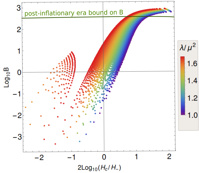
In Figure 8, the top plot of the left panel shows $\gamma$ vs the ratio of the Hubble scale and the upper plot of the right panel shows $\gamma$ vs the decay width where the rainbow color bar shows how these solutions vary with the ratio of $\lambda/\mu^{2}$ . We see from the left panel upper plot that for low Hubble rate we have solutions corresponding to HM instanton which contribute to vacuum decay. Recall that the HM instanton solution is the one for which the inflaton stays at the top of the barrier $X(\rho)=X_{+}$ . This describes the situation where the inflaton climbs up the potential barrier instead of tunneling. On the other hand when the Hubble rate increases i.e. $H_{-}<H_{c}$ , standard CdL solutions appear. On the top left panel of Figure 8, the solutions below the horizontal black line correspond to HM. On the other hand, those solutions which are placed above the black horizontal line correspond to the CdL case. The middle-left panel of Figure 8 shows the plot between the ratio of Hubble scales and the decay rate while on the middle-right panel one can see the value of the potential at both minima. In these scans we only show plots with solutions in which $V(X_{-})>V(X_{0})$ , so the motion of the inflaton field is from right to left. The lower panel shows the plot between the ratio of Hubble scales and the parameter $B$ where as horizontal line in the figure shows the bound on $B$ coming from the post-inflationary era. Based on the numerical value of $B$ we can categorize our false vacuum into stable, meta-stable and unstable. From the plot we see that $B>B_{0}$ (where $B_{0}=540$ ) is a region where $\Gamma<\Gamma_{0}$ and we can infer that false vacuum is stable. Similarly $B\simeq B_{0}$ corresponds to meta-stable and $B<B_{0}$ represents the unstable region.

7 Conclusion

In this work we have investigated various cosmological implications of a generic model based on the extension of the SM gauge symmetry by a $U(1)_{B-L}$ factor, laying special emphasis on the issues of inflation, leptogenesis and baryogenesis as well as the physics of gravitino. The model can be naturally embedded in a unified gauge group with symmetry breaking scale around $M_{GUT}=2\times 10^{16}$ GeV. The spectrum of the model consists of the MSSM content extended by a neutral singlet field $S$ , and a pair of Higgs MSSM singlets $(H,\bar{H})$ carrying opposite charge under $U(1)_{B-L}$ . An appropriate R-symmetry prevents all the dangerous terms in the superpotential whereas a suitable fourth order non-renormalizable term providing Majorana mass to the right-handed neutrino is left intact to realise the seesaw mechanism. The most general effective potential consists of the F- and D-parts as well and contributions coming from soft supersymmetry breaking terms. The F-part arises from the Kähler fucntion, assuming standard no-scale supergravity and the D-terms contain the usual contributions associated with the gauge sector. Under mild constraints on the parameters involved in the scalar potential, it is readily realised that the inflationary scenario is naturally implemented. The cosmological observables, including the tensor-to-scalar ratio $r$ , the spectral index $n_{s}$ etc, are computed and discussed in detail for various limiting cases of the effective potential. In the present analysis, a wide viewpoint is taken, to encompass future perspectives on the possible determination of the supersymmetry breaking scale, $m_{SUSY}$ . Thus, in this context, varying $m_{SUSY}$ from a few TeV up to $10^{6}$ TeV, while fixing the spectral index to its central value $n_{s}=0.9655$ , we find that the tensor-to-scalar ratio lies in the rangle $r\in[10^{-2}-10^{-3}]$ which is consistent with the latest Planck data.

We examine in detail the physics related to the nature of gravitino, considering possible scenarios, including that it is the lightest supersymmetric particle (LSP). Among other possibilities, it is found that a stable LSP gravitino is easily accommodated in our setup and as such, it can be considered as a DM candidate. If the gravitino is not the LSP, it is found that a short lived gravitino is always viable as long as its mass is $m_{3/2}>25$ TeV whereas the mass of a long-lived one should lie in the region $10<m_{3/2}<25$ TeV.

For high SUSY scales the reheating temperature $T_{r}$ is bounded by $\Omega_{LSP}$ whereas for a TeV scale SUSY case the reheating temperature is bounded by BBN predictions. Furthermore the model predicts the inflaton mass to be around $10^{12}$ GeV. On the other hand, the variation of the right-handed heavy Majorana scale depends on $T_{r}$ and ranges between $M_{N}\sim 10^{8}$ and $10^{12}$ GeV. Values close to the upper scale are sufficient to realise the see-saw mechanism and obtain light neutrino masses consistent with the oscillation experiments. Finally we identify regions of the parameter space where the potential in addition to the true vacuum it also displays a false minimum. For this particular case, we discuss quantum tunneling effects with the inflaton field penetrating the barrier, and compute its decay width to the true vacuum using standard techniques developed by Coleman and deLucia [63].

8 Acknowledgements

The authors are thankful to Mansoor Ur Rehman and Fariha K. Vardag for fruitful discussions. The work of GKL was supported by the “Hellenic Foundation for Research and Innovation (H.F.R.I.) under the “First Call for H.F.R.I. Research Projects to support Faculty members and Researchers and the procurement of high-cost research equipment grant” (Project Number: 2251)”.

References

[1] A. A. Starobinsky, Phys. Lett. B 91, 99 (1980); V. F Mukhanov and G.V. Chibisov, JETP Lett. 33, 532 (1981) [Pisma Zh. Eksp. Teor. fiz. 33, 549 (1981)].
[2] A. Guth, Phys. Rev. D 23 (1981) 347-357
[3] A. Albrecht and P. J. Steinhardt, Phys. Rev. Lett. 48,1220 (1982).
[4] P. A. R. Ade et al. [BICEP2 and Keck Array Collaborations], Phys. Rev. Lett. 121, 221301 (2018) [arXiv:1810.05216 [astro-ph.CO]].
[5] Y. Akrami et al. [Planck Collaboration], arXiv:1807.06211 [astro-ph.CO].
[6] J. Ellis, D. V. Nanopoulos and K. A. Olive, Phys. Rev. Lett. 111, 111301 (2013) [Erratum-ibid. 111, no. 12, 129902 (2013)] [arXiv:1305.1247 [hep-th]].
[7] E. Cremmer, S. Ferrara, C. Kounnas and D. V. Nanopoulos, Phys. Lett. B133, 61 (1983).
[8] J. R. Ellis, C. Kounnas and D. V. Nanopoulos, Nucl. Phys.B 247, 373 (1984).
[9] A. B. Lahanas and D. V. Nanopoulos, Phys. Rept. 145, 1 (1987).
[10] M. B. Einhorn and D. R. T. Jones, JHEP 1003, 026 (2010) [arXiv:0912.2718 [hep-ph]].
[11] S. Ferrara, R. Kallosh, A. Linde, A. Marrani and A. Van Proeyen, Phys. Rev. D 83, 025008 (2011) [arXiv:1008.2942 [hep-th]].
[12] S. Ferrara, R. Kallosh, A. Linde, A. Marrani and A. Van Proeyen, Phys. Rev. D 82, 045003 (2010) [arXiv:1004.0712 [hep-th]].
[13] J. Ellis, M. A. G. Garcia, N. Nagata, N. D. V., K. A. Olive and S. Verner, Int. J. Mod. Phys. D 29 (2020) no.16, 2030011 [arXiv:2009.01709 [hep-ph]].
[14] C. Pallis and N. Toumbas, JCAP 1112, 002 (2011) [arXiv:1108.1771 [hep-ph]].
[15] J. Ellis, H. J. He and Z. Z. Xianyu, Phys. Rev. D 91 (2015) no.2, 021302 [arXiv:1411.5537 [hep-ph]].
[16] J. Ellis, H. J. He and Z. Z. Xianyu, JCAP 08 (2016), 068 [arXiv:1606.02202 [hep-ph]].
[17] W. Ahmed and A. Karozas, Phys. Rev. D 98 (2018) no.2, 023538 [arXiv:1804.04822 [hep-ph]].
[18] G. K. Leontaris, N. Okada and Q. Shafi, Phys. Lett. B 765 (2017), 256-259 [arXiv:1611.10196 [hep-ph]].
M. K. Parida, B. P. Nayak, R. Satpathy and R. L. Awasthi, JHEP 04 (2017), 075 [arXiv:1608.03956 [hep-ph]].
A. Karozas, G. K. Leontaris, Q. Shafi, I. Tavellaris, in preparation.
[19] H. M. Lee, JCAP 1008, 003 (2010) doi:10.1088/1475-7516/2010/08/003 [arXiv:1005.2735 [hep-ph]].
[20] F. L. Bezrukov, A. Magnin and M. Shaposhnikov, Phys. Lett. B 675, 88 (2009) [arXiv:0812.4950 [hep-ph]]; A. De Simone, M. P. Hertzberg and F. Wilczek, Phys. Lett. B 678, 1 (2009) [arXiv:0812.4946 [hep-ph]]; A. O. Barvinsky, A. Y. Kamenshchik, C. Kiefer, A. A. Starobinsky and C. Steinwachs, JCAP 0912, 003 (2009) [arXiv:0904.1698 [hep-ph]]; N. Okada, M. U. Rehman and Q. Shafi, arXiv:0911.5073 [hep-ph].
[21] N. Okada, M. U. Rehman and Q. Shafi, Phys. Rev. D 82, 043502 (2010) [arXiv:1005.5161 [hep-ph]]; A. Linde, M. Noorbala and A. Westphal, JCAP 1103, 013 (2011) [arXiv:1101.2652 [hep-th]]; N. Okada, M. U. Rehman and Q. Shafi, Phys. Lett. B 701, 520 (2011) [arXiv:1102.4747 [hep-ph]]; C. Pallis and Q. Shafi, JCAP 1503, no. 03, 023 (2015) [arXiv:1412.3757 [hep-ph]]; N. Bostan, Ö. Güleryüz and V. N. Şenoğuz, JCAP 1805, no. 05, 046 (2018) [arXiv:1802.04160 [astro-ph.CO]]; N. Bostan and V. N. Senoguz, arXiv:1907.06215 [astro-ph.CO].
[22] A. R. Liddle and D. H. Lyth, “Cosmological inflation and large scale structure,”
[23] A. D. Linde, Phys. Rev. D 49 (1994), 748-754 [arXiv:astro-ph/9307002 [astro-ph]].
[24] G. R. Dvali, Q. Shafi and R. K. Schaefer, Phys. Rev. Lett. 73, 1886 (1994) [hep-ph/9406319].
[25] E. J. Copeland, A. R. Liddle, D. H. Lyth, E. D. Stewart and D. Wands, Phys. Rev. D 49, 6410 (1994) [astro-ph/9401011].
[26] A. D. Linde and A. Riotto, Phys. Rev. D 56, R1841 (1997) [hep-ph/9703209]; V. N. Senoguz and Q. Shafi, Phys. Rev. D 71, 043514 (2005) [hep-ph/0412102]; M. U. Rehman, Q. Shafi and J. R. Wickman, Phys. Lett. B 683, 191 (2010) [arXiv:0908.3896 [hep-ph]].
[27] R. Jeannerot, S. Khalil, G. Lazarides and Q. Shafi, JHEP 0010, 012 (2000) [hep-ph/0002151].
[28] G. Lazarides and C. Panagiotakopoulos, Phys. Rev. D 52, R559 (1995) [hep-ph/9506325].
[29] N. Arkani-Hamed and S. Dimopoulos, JHEP 06 (2005), 073 [arXiv:hep-th/0405159 [hep-th]].
[30] G. F. Giudice and A. Romanino, Nucl. Phys. B 699 (2004), 65-89 [erratum: Nucl. Phys. B 706 (2005), 487-487] [arXiv:hep-ph/0406088 [hep-ph]].
[31] W. Buchmuller, V. Domcke and K. Schmitz, Nucl. Phys. B 862 (2012), 587-632 [arXiv:1202.6679 [hep-ph]].
[32] W. Buchmuller, V. Domcke, K. Kamada and K. Schmitz, [arXiv:1309.7788 [hep-ph]].
[33] W. Ahmed, S. Raza, Q. Shafi, C. S. Un and B. Zhu, JHEP 01 (2021), 161 [arXiv:2008.01568 [hep-ph]].
[34] G. R. Dvali, G. Lazarides and Q. Shafi, Phys. Lett. B 424, 259-264 (1998) [arXiv:hep-ph/9710314 [hep-ph]].
[35] S. F. King and Q. Shafi, Phys. Lett. B 422, 135-140 (1998) [arXiv:hep-ph/9711288 [hep-ph]].
[36] R. Deen, B. A. Ovrut and A. Purves, Phys. Lett. B 762 (2016), 441-446 [arXiv:1606.00431 [hep-ph]].
[37] G. F. Giudice and A. Masiero, Phys. Lett. B 206 (1988), 480-484
[38] W. Buchmuller, L. Covi and D. Delepine, Phys. Lett. B 491 (2000), 183-189 [arXiv:hep-ph/0006168 [hep-ph]].
[39] W. Buchmüller, V. Domcke, K. Kamada and K. Schmitz, JCAP 07 (2014), 054 [arXiv:1404.1832 [hep-ph]].
[40] W. Buchmuller, V. Domcke, H. Murayama and K. Schmitz, Phys. Lett. B 809 (2020), 135764 [arXiv:1912.03695 [hep-ph]].
[41] C. Pallis, Universe 4, no.1, 13 (2018) [arXiv:1710.05759 [hep-ph]]; C. Pallis and Q. Shafi, Eur. Phys. J. C 78, no.6, 523 (2018) [arXiv:1803.00349 [hep-ph]].
[42] M. Y. Khlopov and A. D. Linde, Phys. Lett. B 138, 265-268 (1984)
[43] J. R. Ellis, J. E. Kim and D. V. Nanopoulos, Phys. Lett. B 145, 181-186 (1984)
[44] M. Kawasaki and T. Moroi, Prog. Theor. Phys. 93, 879-900 (1995) [arXiv:hep-ph/9403364 [hep-ph]].
[45] R. H. Cyburt, J. R. Ellis, B. D. Fields and K. A. Olive, Phys. Rev. D 67, 103521 (2003) [arXiv:astro-ph/0211258 [astro-ph]].
[46] M. Fujii, M. Ibe and T. Yanagida, Phys. Lett. B 579, 6-12 (2004) [arXiv:hep-ph/0310142 [hep-ph]].
[47] T. Gherghetta, G. F. Giudice and A. Riotto, Phys. Lett. B 446, 28-36 (1999) [arXiv:hep-ph/9808401 [hep-ph]].
[48] T. Gherghetta, G. F. Giudice and J. D. Wells, Nucl. Phys. B 559, 27-47 (1999) [arXiv:hep-ph/9904378 [hep-ph]].
[49] P. Andre et al. [PRISM], [arXiv:1306.2259 [astro-ph.CO]].
[50] T. Matsumura et al., “Mission design of LiteBIRD,” J. Low Temp. Phys. 176, 733 (2014) [arXiv:1311.2847 [astro-ph.IM]].
[51] A. Kogut et al., JCAP 07, 025 (2011) [arXiv:1105.2044 [astro-ph.CO]].
[52] F. Finelli et al. [CORE], JCAP 04, 016 (2018) [arXiv:1612.08270 [astro-ph.CO]].
[53] G. Lazarides, M. U. Rehman, Q. Shafi and F. K. Vardag, Phys. Rev. D 103 (2021) no.3, 035033 [arXiv:2007.01474 [hep-ph]].
[54] N. Okada and Q. Shafi, Phys. Lett. B 775, 348-351 (2017) [arXiv:1506.01410 [hep-ph]].
[55] M. Bolz, A. Brandenburg and W. Buchmuller, Nucl. Phys. B 606, 518-544 (2001) [arXiv:hep-ph/0012052 [hep-ph]].
[56] J. Pradler and F. D. Steffen, Phys. Rev. D 75 (2007), 023509 [arXiv:hep-ph/0608344 [hep-ph]].
[57] V. S. Rychkov and A. Strumia, Phys. Rev. D 75 (2007), 075011 [arXiv:hep-ph/0701104 [hep-ph]].
[58] H. Eberl, I. D. Gialamas and V. C. Spanos, Phys. Rev. D 103 (2021) no.7, 075025 [arXiv:2010.14621 [hep-ph]].
[59] T. A. Vami [ATLAS and CMS], PoS LHCP2019, 168 (2019) [arXiv:1909.11753 [hep-ex]].
[60] M. Aaboud et al. [ATLAS], Phys. Rev. D 97, no.11, 112001 (2018) [arXiv:1712.02332 [hep-ex]].
[61] M. Kawasaki, K. Kohri and T. Moroi, Phys. Rev. D 71, 083502 (2005) [arXiv:astro-ph/0408426 [astro-ph]]; M. Kawasaki, K. Kohri, T. Moroi and A. Yotsuyanagi, Phys. Rev. D 78 (2008), 065011 [arXiv:0804.3745 [hep-ph]]; M. Kawasaki, K. Kohri, T. Moroi and Y. Takaesu, Phys. Rev. D 97, no.2, 023502 (2018) [arXiv:1709.01211 [hep-ph]]
[62] D. Hooper and T. Plehn, Phys. Lett. B 562, 18-27 (2003) [arXiv:hep-ph/0212226 [hep-ph]].
[63] S. R. Coleman and F. De Luccia, “Gravitational Effects on and of Vacuum Decay,” Phys. Rev. D 21 (1980), 3305
[64] T. Markkanen, A. Rajantie and S. Stopyra, Front. Astron. Space Sci. 5 (2018), 40 [arXiv:1809.06923 [astro-ph.CO]].
[65] I. Antoniadis, O. Lacombe and G. K. Leontaris, Eur. Phys. J. C 80 (2020) no.11, 1014 [arXiv:2007.10362 [hep-th]].
[66] S. W. Hawking and I. G. Moss, “Supercooled Phase Transitions in the Very Early Universe,” Adv. Ser. Astrophys. Cosmol. 3 (1987), 154-157