Exceptional Degeneracy in a Waveguide Periodically Loaded with Discrete Gain and Radiation Loss Elements
Abstract
We demonstrate that a periodic waveguide comprising of uniform lossless segments together with discrete gain and radiating elements supports exceptional points of degeneracy (EPDs). We provide analytical expressions for all possible conditions that guarantee the occurrence of an EPD, i.e., the coalescence of eigenvalues and eigenvectors. We show that EPDs are not only achieved using symmetric gain and radiation periodic loading, but they are also obtained using asymmetric gain and radiation loss conditions. We illustrate the characteristics of the degenerate electromagnetic modes, showing the dispersion diagram and discussing the tunability of the EPD frequency. We show a special condition, we refer to it as parity-time (PT)-glide symmetry, which leads to a degeneracy that is occurring at all frequencies of operation. The class of EPDs proposed in this work is very promising for many applications that incorporate discrete-distributed coherent sources and radiation-loss elements; operating in the vicinity of such special degeneracy conditions leads to potential performance enhancement in a variety of microwave and optical resonators, antennas, and devices and can be extended to a new class of active integrated antenna arrays and radiating laser arrays.
Index Terms:
periodic structures, exceptional points, dispersion engineering, parity-time symmetry, transmission lineElectromagnetic (EM) guiding structures or resonators are described by their eigenmodes’ (eigenvalues and eigenvectors) evolution equations. Eigenmodes representing EM propagating waves in a multimodal waveguide may coalesce into a single degenerate eigenmode by varying at least one parameter of the parameter space (frequency, geometrical/physical parameters) of the waveguide system; this special point in the system parameter space is called an exceptional point of degeneracy (EPD) [1, 2]. At the EPD, two or more eigenstates of the system coalesce into a single degenerate eigenstate. Such condition is simply referred to as ’EP’ in various works; here the ‘D’ is used to stress the importance of degeneracy [3]. The number of degenerated eigenstates is referred to as the order of the exceptional point. In the proximity of an EPD angular frequency , the eigenvalues associated with the coalescing eigenvectors change with respect to frequency as , in which , and are the degenerate eigenvalue, EPD angular frequency, and order of EPD, respectively.
In general, an EPD occurs in a system where the space-time evolution of the system vector is characterized by a non-Hermitian matrix, which can be imposed also by periodicity in space [4, 5, 6, 7] or in time [8, 9] or by having losses and gain in the system [10, 7] including systems satisfying parity-time (PT) symmetry [2, 11, 12]. The unique degenerate dispersion behavior is accompanied by supreme characteristics including the vanishing of the group velocity [13, 14] as well as the dramatic improvement in the local density of states [15] resulting in a robust increase in the loaded quality factor of the structure. The EPD phenomenon has been proved to have various applications including high quality factor () and low-threshold lasers [16], lasers in coupled ring resonators[17], and low-threshold oscillators [18, 19, 20]. Moreover, the deviation of the perturbed eigenvalues from the degenerate eigenvalue is large when a small perturbation to a system parameter is applied; so this sensitivity brings another class of applications in sensors [21, 22, 23, 24].
In this paper, we present an example of a waveguide that exhibits a second-order EPD by periodically loading a uniform waveguide with gain and radiating elements, as schematized in Fig. 1. We provide the analytical expressions for the second-order EPD conditions to occur in different loading configurations for the gain and radiating elements. The EPD condition is observed in the dispersion diagram and by the coalescence of the eigenvectors. We also describe the Floquet-Bloch impedance in the vicinity of the EPD, which can be important for matching and stability analysis. We conclude by showing a possible application as an array of radiation elements oscillating and radiating at the EPD frequency.
We consider a uniform waveguide that is periodically loaded with discrete gain and loss and that is schematically represented by its equivalent transmission line model (TL) [25, 26]; this model can be applied to waveguides operating from microwaves to optics, hence our formulation is general. We assume that the waveguide is periodically loaded with discrete shunt gain and resistive elements, as shown in Fig. 1(a). Indeed, it is customary to represent radiation from discrete points along a waveguide using resistive loads.
The periodic unit cell is divided into four parts: two uniform waveguide segments together with a discrete gain element and a discrete radiative element represented by its equivalent resistance. For simplicity the waveguide segments are assumed to have similar characteristic impedance, but with possibly different electrical lengths , and where and are the physical lengths of the waveguide segments A and B, respectively, and is the waveguide propagation constant, with being the phase velocity of a uniform-waveguide mode. It is convenient to define a system state vector as , with indicating the transpose action. Therefore, referring to Fig. 1(a), we use the transfer matrix of a shunt element and lossless transmission line [27], and we form a relation between equivalent voltage and current between the two ends of a unit cell as . The unit cell transfer matrix is the result of the multiplication of four transfer matrices as
| (1) |
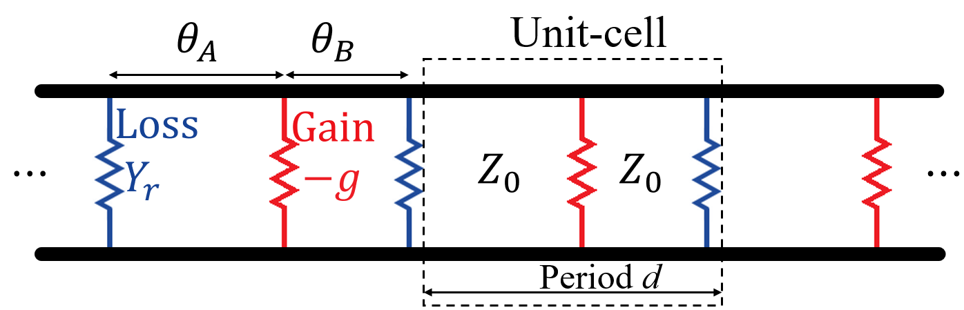
We look for solutions of the type satisfying the Floquet’s condition , where is the waveguide period, is the Floquet-Bloch wavenumber, and we implicitly assume the time convention . Hence, the eigenmodes supported in such a system are described by the eigenvalue problem
| (2) |
where is the identity matrix of order two, is an eigenvalue and is the associated eigenvector. The eigenvalues are readily found by solving the characteristic equation , i.e., by finding the roots of the characteristic polynomial
| (3) |
where is the characteristic impedance of the two uniform waveguide segments. To have two identical roots in a second-order polynomial of the form of , must vanish. Having in the proposed system characteristic polynomial (3) indicates that the eigenvalues are , which implies that . Also, the necessary and sufficient conditions for having identical eigenvalues is where is an integer number indicating the positive and negative possible solutions of . Therefore conditions that must be satisfied at the EPD frequency, related to the real and imaginary parts of , read as
| (4) |
| (5) |
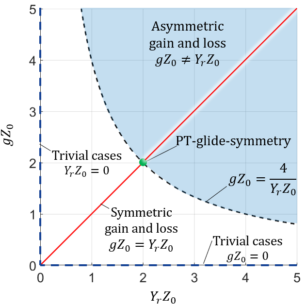
The second condition, (5), is satisfied either by constraining the gain and radiation-element equivalent resistance (i.e., ) or by constraining the TL segments’ electrical lengths (i.e., ). Whereas, the first condition in (4) is used as the design equation for different possible cases that are leading to identical eigenvalues. The chart in Fig. 1(b) summarizes the required relation between gain and radiation loss to have an EPD, that are discussed next.
Trivial cases with vanishing gain or loss ( or
A trivial condition to satisfy EPD is by having where is an integer, besides having either or , represented by the blue-dashed vertical or horizontal line, respectively, in the chart in Fig. 1(b). The EPD obtained for this case occurs at , where is the unit cell period. However, we do not focus on this trivial case as it is not suitable for applications that incorporate both discrete-distributed coherent sources and radiation loss elements.
Symmetric gain and loss cases
One possibility to satisfy the condition in (5), , is by enforcing balanced gain and radiation-loss, represented by the solid-red line in the chart in Fig. 1(b). The normalized gain and radiation elements values that satisfy the other EPD condition (4) , yields
| (6) |
It is important to mention that for any arbitrary choice of and the term inside the root in (6) can always have a positive value by choosing the proper value. The symmetrical gain and radiation-loss is a straightforward condition that leads to EPD where the introduced amount of radiation loss should be compensated with the same amount of gain in order to have neither a decaying nor a growing wave. Although, in this case, gain and loss loads are equal, the unit cell with does not classify as (PT)-symmetric condition, that could be defined based on the system’s refractive index obeying , where is a coordinate in the system and denotes complex conjugation [28, 11, 2]. Enforcing spatial symmetry in the unit cell by choosing equal electrical lengths leads to a unit cell that satisfies a possible definition of PT-symmetry as used in [29]. Indeed, the symmetric load case with satisfies the following
| (7) |
which holds the reflection between gain and loss by the complex conjugate operator and the translation along by half a period. We define the PT-glide-symmetry condition as in (7) which can be used also to describe more complicated structures. In general, glide symmetry is a symmetry operation comprised of a reflection operation over a certain coordinate and translation along with that coordinate [30, 31, 32]. We refer to the condition in (7) as PT-glide-symmetry where the EPD condition met at every frequency with . Note that for the reciprocal system we are studying, the EPD is only possible when is purely real with the value of either or .
Figure 2 depicts the dispersion of a waveguide with symmetric loads and different electrical lengths. The waveguide exhibits EPD by satisfying the EPD condition in (6) at GHz such that , , and S.

In the rest of the paper, we focus on the case with asymmetric gain and radiation-loss as it provides more flexibility in using different values of gain and radiation-loss. Indeed, the value of resistance of the radiating element cannot be set arbitrarily and the constraints depend on the specific design, while gain usually can be tuned by simply changing a biasing voltage.
Asymmetric gain and loss cases
Condition (5) can be satisfied also for asymmetric gain and radiation-loss cases, represented by the shaded area in the chart in Fig. 1(b), by constraining the waveguide segments’ electrical lengths as
| (8) |
where is an integer number, in other words, the total length of the waveguide of a unit cell at is an integer multiple of half wavelength. The other condition (4) forces the relation between the normalized gain and radiation-loss values to be
| (9) |
By forcing these two conditions (8,9), the degenerate eigenvalue of the eigenvalue problem in (2) is equal to
| (10) |
where is an integer such that , and the degenerate eigenvector is , where
| (11) |
is the Bloch impedance of the degenerate mode. Figure 3(a) depicts the dispersion of one waveguide that exhibits EPD by satisfying the conditions at GHz such that , mS, , and mS to satisfy the EPD condition in (9). The two complex wavenumbers are traced in two different colors such that one can observe the coalescence of the two complex wavenumbers at the EPD frequency and its harmonics (i.e. all meet the EPD conditions). Note that the EPD points are the transition points at which the complex wavenumbers alternate between the same sign for both parties of the complex wavenumber (i.e. real and imaginary parts) indicating growing waves to opposite signs indicating decaying waves.
Upon analyzing the modal dispersion equation, it can be proved that when the special case of , accordingly, (i.e., symmetric case) and are met utilizing the aforementioned PT-glide-symmetry case, then the two eigenvalues (and also the eigenvectors) will be identical at every frequency. In Fig. 3(a) we show an example of the dispersion when when , that is true when using the aforementioned parameters, whereas in Fig. 3(b) we show an analogous example that exhibits EPD at the same frequency when the condition reads as by selecting 50 mS and mS for the same .


The periodic electromagnetic guiding structure is characterized by the modal dispersion equations (3). Each eigenmode is characterized by its eigenvalue related to the associated complex Floquet wavenumbers and its eigenvector , with for the case under study here, where is the mode Floquet-Bloch impedance.
The evolution of the eigenmodes’ complex Floquet-Bloch impedance varying frequency, which is directly related to the evolution of the eigenvectors , is shown next. The coalescence of the eigenvectors at the EPD is based on having a degenerate Floquet-Bloch impedance (i.e., ). Figure 4 shows the trajectory of the complex Bloch impedance for increasing frequency for two different cases: (a) depicted in Fig. 4(a), and (b) depicted in Fig. 4(b), associated with dispersion diagrams shown in Fig. 3(a,b), respectively. It is obvious from the traces shown in Fig. 4(a,b) that in general, the Bloch impedances are complex conjugate to each other over the whole frequency range except at the EPD frequency GHz and its harmonics GHz where they become purely real. At the EPD, the two impedances turn into one degenerate real impedance either or zero.

We describe succinctly some possible applications that incorporate discrete-distributed coherent sources and radiation elements (that are usually characterized by loss lumped elements, like the admittances ). One application to the proposed EPD scheme is an active radiating oscillator that requires the incorporation of discrete-distributed coherent sources and radiation loss elements. This active oscillator is realized in a cavity made of a finite-length waveguide exhibiting EPD with asymmetric gain and loss. As proof of the concept, and regardless of the specific implementation, the radiating elements are simply modeled as a distributed shunt radiation loss, whereas gain is modeled in each unit cell using non-linear cubic characteristic of the active device [33, 20] which can be practically implemented with circuits with amplifying devices, such as CMOS transistors or Op-Amps, with positive feedback. Here is the small-signal slope of the curve in the negative resistance region, and is the third-order non-linearity constant that models the saturation characteristic of the device. We set the turning point of the characteristics to be volt, and accordingly, we set .
We tested the finite-length loaded cavity comprised of 8 unit cells as shown in Fig. 5(a) in the time domain solver implemented in Cadence Virtuoso IC 616. The unit cell is chosen to have identical ideal TL segments with and each has an electric length . The gain and loss elements are chosen as mS, mS to satisfy the EPD condition in (9). Accordingly, we report that the oscillation occurs close to the EPD frequency and the waveform , at the load in the middle of the structure between the fourth and the fifth unit cell reaches a steady-state in less than 2 ns as shown in Fig. 5(b). The oscillation frequency is determined by taking the Fourier transform of in the time window from 2 to 100 ns, shown in Fig. 5(c), and it confirms the oscillatory behavior around the EPD frequency 3 GHz and its odd harmonics (9, 15, …) GHz since they all satisfy EPD conditions.

In summary, we have demonstrated that a periodic waveguide loaded with gain and radiating elements as shown in Fig. 1(a) exhibits EPDs. We have shown the different conditions for having EPDs summarized in Fig. 1(b) and also, importantly, we have demonstrated a case where the EPD condition is met at every frequency satisfying the PT-glide-symmetry condition. The theoretical framework developed applies to various structures operating from microwave to optical frequencies. The discrete radiation admittances considered in this paper represent the input admittances of a periodic array of antennas. We have shown that EPDs occur at frequencies where the two TL wavenumbers vanish, leading to possible applications of broadside radiation in arrays of antennas periodically connected to the waveguide. Such a phenomenon may pave the way to a new class of active traveling-wave antennas and also in array antennas with all elements oscillating and synchronized.
Acknowledgment
This material is based upon work supported by the National Science Foundation under award NSF ECCS-1711975.
References
- [1] T. Kato, Perturbation theory for linear operators. springer, 1995, vol. 132.
- [2] W. D. Heiss, “The physics of exceptional points,” Journal of Physics A: Mathematical and Theoretical, vol. 45, no. 44, p. 444016, 2012.
- [3] M. V. Berry, “Physics of nonhermitian degeneracies,” Czechoslovak journal of physics, vol. 54, no. 10, pp. 1039–1047, 2004.
- [4] A. Figotin and I. Vitebskiy, “Gigantic transmission band-edge resonance in periodic stacks of anisotropic layers,” Physical Review E, vol. 72, no. 3, p. 036619, Sep. 2005.
- [5] M. A. K. Othman, X. Pan, Y. Atmatzakis, and C. G. Christodoulou, “Experimental Demonstration of Degenerate Band Edge in Metallic Periodically-Loaded Circular Waveguide,” IEEE Microwave Theory and Techniques, vol. 1611, no. 8, p. 9, 2017.
- [6] A. Figotin and I. Vitebskiy, “Slow-wave resonance in periodic stacks of anisotropic layers,” Physical Review A, vol. 76, no. 5, p. 053839, Nov 2007.
- [7] A. F. Abdelshafy, M. A. K. Othman, D. Oshmarin, A. Al-Mutawa, and F. Capolino, “Exceptional Points of Degeneracy in Periodically-Coupled Waveguides and the Interplay of Gain and Radiation Loss: Theoretical and Experimental Demonstration,” IEEE Transactions on Antennas and Propagation, vol. 67, no. 09, 2019.
- [8] H. Kazemi, M. Y. Nada, T. Mealy, A. F. Abdelshafy, and F. Capolino, “Exceptional Points of Degeneracy Induced by Linear Time-Periodic Variation,” Physical Review Applied, vol. 11, no. 1, p. 014007, Jan. 2019.
- [9] K. Rouhi, H. Kazemi, A. Figotin, and F. Capolino, “Exceptional Points of Degeneracy Directly Induced by Space-Time Modulation of a Single Transmission Line,” arXiv:2004.11423 [physics], Apr. 2020, arXiv: 2004.11423.
- [10] M. A. K. Othman and F. Capolino, “Theory of Exceptional Points of Degeneracy in Uniform Coupled-Waveguides and Balance of Loss and Gain,” IEEE Transactions on Antennas and Propagation, vol. 65, no. 10, pp. 1–15, 2017.
- [11] C. E. Rüter, K. G. Makris, R. El-Ganainy, D. N. Christodoulides, M. Segev, and D. Kip, “Observation of parity-time symmetry in optics,” Nature Physics, vol. 6, no. 3, pp. 192–195, 2010.
- [12] A. Guo, G. J. Salamo, D. Duchesne, R. Morandotti, M. Volatier-Ravat, V. Aimez, G. A. Siviloglou, and D. N. Christodoulides, “Observation of P T-symmetry breaking in complex optical potentials,” Physical Review Letters, vol. 103, no. 9, p. 093902, 2009.
- [13] A. Figotin and I. Vitebskiy, “Frozen light in photonic crystals with degenerate band edge,” Physical Review E, vol. 74, no. 6, p. 066613, Dec. 2006.
- [14] N. Gutman, C. M. de Sterke, A. A. Sukhorukov, and L. C. Botten, “Slow and frozen light in optical waveguides with multiple gratings: Degenerate band edges and stationary inflection points,” Physical Review A, vol. 85, no. 3, p. 033804, 2012.
- [15] M. A. K. Othman, F. Yazdi, A. Figotin, and F. Capolino, “Giant gain enhancement in photonic crystals with a degenerate band edge,” Physical Review B, vol. 93, no. 2, p. 024301, Jan. 2016.
- [16] M. Veysi, M. A. K. Othman, A. Figotin, and F. Capolino, “Degenerate band edge laser,” Physical Review B, vol. 97, no. 19, p. 195107, May 2018.
- [17] H. Hodaei, M.-A. Miri, M. Heinrich, D. N. Christodoulides, and M. Khajavikhan, “Parity-time-symmetric microring lasers,” Science, vol. 346, no. 6212, pp. 975–978, 2014.
- [18] M. A. Othman, M. Veysi, A. Figotin, and F. Capolino, “Low Starting Electron Beam Current in Degenerate Band Edge Oscillators,” IEEE Transactions on Plasma Science, vol. 44, no. 6, pp. 918–929, 2016.
- [19] A. F. Abdelshafy, M. A. Othman, F. Yazdi, M. Veysi, A. Figotin, and F. Capolino, “Electron-Beam-Driven Devices With Synchronous Multiple Degenerate Eigenmodes,” IEEE Transactions on Plasma Science, vol. 46, no. 8, pp. 3126–3138, 2018.
- [20] A. F. Abdelshafy, D. Oshmarin, M. A. K. Othman, M. M. Green, and F. Capolino, “Distributed degenerate band edge oscillator,” IEEE Transactions on Antennas and Propagation, vol. 69, no. 3, pp. 1821–1824, 2021.
- [21] J. Wiersig, “Sensors operating at exceptional points: General theory,” Physical Review A, vol. 93, no. 3, p. 033809, 2016.
- [22] H. Hodaei, A. U. Hassan, S. Wittek, H. Garcia-Gracia, R. El-Ganainy, D. N. Christodoulides, and M. Khajavikhan, “Enhanced sensitivity at higher-order exceptional points,” Nature, vol. 548, no. 7666, pp. 187–191, 2017.
- [23] J. Ren, H. Hodaei, G. Harari, A. U. Hassan, W. Chow, M. Soltani, D. Christodoulides, and M. Khajavikhan, “Ultrasensitive micro-scale parity-time-symmetric ring laser gyroscope,” Optics Letters, vol. 42, no. 8, pp. 1556–1559, Apr. 2017.
- [24] H. Kazemi, A. Hajiaghajani, M. Y. Nada, M. Dautta, M. Alshetaiwi, P. Tseng, and F. Capolino, “Ultra-Sensitive Radio Frequency Biosensor at an Exceptional Point of Degeneracy induced by Time Modulation,” arXiv:1909.03344 [physics], Jul. 2020, arXiv: 1909.03344.
- [25] N. Marcuvitz and J. Schwinger, “On the representation of the electric and magnetic fields produced by currents and discontinuities in wave guides. I,” Journal of Applied Physics, vol. 22, no. 6, pp. 806–819, 1951.
- [26] L. B. Felsen and N. Marcuvitz, Radiation and scattering of waves. John Wiley & Sons, 1994, vol. 31.
- [27] D. M. Pozar, Microwave engineering. John Wiley & Sons, 2009.
- [28] R. El-Ganainy, K. G. Makris, D. N. Christodoulides, and Z. H. Musslimani, “Theory of coupled optical PT-symmetric structures,” Optics letters, vol. 32, no. 17, pp. 2632–2634, 2007.
- [29] H. Wu, X. Yang, Y. Tang, X. Tang, D. Deng, H. Liu, and Z. Wei, “The Scattering Problem in PT-Symmetric Periodic Structures of 1D Two-Material Waveguide Networks,” Annalen der Physik, vol. 531, no. 9, 2019.
- [30] A. Hessel, M. H. Chen, R. C. Li, and A. A. Oliner, “Propagation in periodically loaded waveguides with higher symmetries,” Proceedings of the IEEE, vol. 61, no. 2, pp. 183–195, 1973.
- [31] M. Bagheriasl, O. Quevedo-Teruel, and G. Valerio, “Bloch analysis of artificial lines and surfaces exhibiting glide symmetry,” IEEE Transactions on Microwave Theory and Techniques, vol. 67, no. 7, pp. 2618–2628, 2019.
- [32] A. Mock, “Symmetry-engineered waveguide dispersion in pt symmetric photonic crystal waveguides,” J. Opt. Soc. Am. B, vol. 37, no. 1, pp. 168–180, Jan 2020.
- [33] D. Oshmarin, F. Yazdi, M. A. Othman, J. Sloan, M. Radfar, M. M. Green, and F. Capolino, “New oscillator concept based on band edge degeneracy in lumped double-ladder circuits,” IET Circuits, Devices & Systems, vol. 13, no. 7, pp. 950–957, 2019.