RLIBM-32: High Performance Correctly Rounded Math Libraries for 32-bit
Floating Point Representations
Rutgers Department of Computer Science Technical Report DCS-TR-754
Extended version of the PLDI 2021 paperConference: Rutgers DCS Technical Report DCS-TR-754; 2021CCS: Mathematics of computing Mathematical softwareCCS: Theory of computation Numeric approximation algorithmsCCS: Mathematics of computing Linear programming
Abstract.
This paper proposes a set of techniques to develop correctly rounded math libraries for 32-bit float and posit types. It enhances our RLibm approach that frames the problem of generating correctly rounded libraries as a linear programming problem in the context of 16-bit types to scale to 32-bit types. Specifically, this paper proposes new algorithms to (1) generate polynomials that produce correctly rounded outputs for all inputs using counterexample guided polynomial generation, (2) generate efficient piecewise polynomials with bit-pattern based domain splitting, and (3) deduce the amount of freedom available to produce correct results when range reduction involves multiple elementary functions. The resultant math library for the 32-bit float type is faster than state-of-the-art math libraries while producing the correct output for all inputs. We have also developed a set of correctly rounded elementary functions for 32-bit posits.
Keywords:
correctly rounded math libraries, elementary functions, floating point, posits, piecewise polynomials1. Introduction
Math libraries provide implementations of elementary functions (e.g. , , ) (Muller 2005). They are crucial components in various domains ranging from scientific computing to machine learning. Designing math libraries is a challenging task because they are expected to provide correct results for all inputs and also have high performance. These elementary functions are typically approximated with some hardware supported representation for performance.
Given a representation with finite precision (e.g., float), the correctly rounded result of an elementary function for an input is defined as the value of computed with real numbers and then rounded to a value in the representation . The IEEE-754 standard recommends the generation of correctly rounded results for elementary functions. Seminal prior work on generating approximations for elementary functions has resulted in numerous implementations that have reduced error significantly (Lefèvre et al. 1998; Chevillard et al. 2010; Brisebarre et al. 2006; Chevillard and Lauter 2007; Chevillard et al. 2011; Kupriianova and Lauter 2014; Brunie et al. 2015; Jeannerod et al. 2011; Bui and Tahar 1999; Ziv 1991; Fousse et al. 2007). Further, numerous correctly rounded libraries have also been developed (Daramy-Loirat et al. 2006; Fousse et al. 2007). Unfortunately, they are not widely used due to performance considerations. Moreover, widely used libraries do not produce correct results for all inputs.
Mini-max approaches. Most prior approaches identify a polynomial that minimizes the maximum error among all input points (i.e., a mini-max approach) compared to the real value of the elementary function using the Weierstrass approximation theorem and the Chebyshev alternation theorem (Trefethen 2012). The Weierstrass approximation theorem states that if is a continuous real-valued function on and , there exists a polynomial such that for all . The Chebyshev alternation theorem provides the condition for such a polynomial: a polynomial of degree that minimizes the maximum error will have at least points where it has the absolute maximum error and the error alternates in sign. Remez algorithm (Remes 1934; Muller 2005) is a procedure to identify such mini-max polynomials. The maximum approximation error has to be below the error threshold required to produce correct results for all inputs.
As approximating a polynomial in a small domain is much easier, the input domain of the function is reduced using range reduction (Cody and Waite 1980; Tang 1990; Lim et al. 2020a). The approximated result is adjusted to produce the result for the original input (i.e., output compensation). Both range reduction and polynomial evaluation in a representation with finite precision will have some numerical errors. The combination of approximation errors with the mini-max approach and numerical errors with polynomial evaluation, range reduction, and output compensation can result in wrong results.

RLibm. Our RLibm approach (Lim et al. 2021; Lim et al. 2020a) generates polynomials that approximate the correctly rounded result rather than the real value of the elementary function. The generation of the polynomial considers errors in polynomial approximation and numerical errors in polynomial evaluation, range reduction, and output compensation to produce the correctly rounded output for all inputs. The task of generating the polynomial is then structured as a linear programming (LP) problem. The RLibm approach first computes the correctly rounded result for each input in a target representation using an oracle (e.g., the MPFR library (Fousse et al. 2007)). Given the correctly rounded result for an input, it finds an interval in double precision such that every value in the interval rounds to the correctly rounded result, which is called the rounding interval. The rounding intervals are further constrained to account for numerical errors during range reduction and output compensation. Subsequently, it attempts to generate a polynomial of degree using an LP solver, which when evaluated with an input produces a result that lies within the rounding interval. Using the RLibm approach, we have been successful in generating correctly rounded libraries with 16-bit types such as bfloat16 and posit16.
Challenges in scaling to 32-bits. To extend our RLibm approach to 32-bit data types, we have to address the following challenges. First, modern LP solvers can handle a few thousand constraints. A naive use of the RLibm approach with 32-bit types will generate more than a billion constraints, which is beyond the capabilities of current LP solvers. Second, it may not be feasible to generate a single polynomial of a reasonable degree given the large number of constraints. Third, LP solvers are sensitive to the condition number of the system of constraints. LP solvers will not be able to solve an ill-conditioned system of constraints. An effective range reduction is a strategy to address it. Although there are excellent books on range reduction (Cody and Waite 1980), these techniques need to be adapted to work with our RLibm approach. Fourth, some range reduction strategies need multiple elementary functions themselves (e.g., ). Finally, we need to ensure that output compensation does not experience pathological cancellation errors (e.g., ).
This paper. Our goal is to generate efficient implementations of elementary functions that produce correctly rounded results for all inputs with 32-bit types. This paper extends our RLibm approach to scale to 32-bit FP types to address the challenges described above. We propose (1) sampling of inputs with counterexample guided polynomial generation to handle the large input space, (2) generation of piecewise polynomials for efficiency, (3) deduction of rounding intervals when a range reduction technique uses multiple elementary functions, and (4) modified range reduction techniques for some elementary functions to address cancellation errors in output compensation. Figure 1 pictorially represents our approach to scale to 32-bit data types.
Counterexample guided polynomial generation. We sample inputs proportional to the number of representable values in a given input domain with a 32-bit representation . To generate polynomials that produce the correctly rounded result for every input, it is not necessary to consider every input and its rounding interval. We primarily need to consider those rounding intervals that are highly constrained. For each input in the sample, we generate the oracle result using the MPFR library. We compute the rounding interval in double precision (i.e., set of values in the double type that round to the oracle result). We generate LP constraints to create a polynomial of degree such that it evaluates to a value in the rounding interval for each input in the sample. If the initial sample generates a polynomial that produces the correctly rounded output for all values in , then the process terminates. Otherwise, we add counterexamples to the sample and repeat the process. The size of the sample is bounded by the number of constraints that the LP solver can process.
Piecewise polynomials. When either the number of inputs in the sample exceeds our LP constraint threshold or the LP solver is not able to generate a polynomial, we split the input domain to and to generate piecewise polynomials using the above process for each input sub-domain. We choose the splitting point such that we can identify the sub-domain quickly using a few bits of the input, which results in efficient implementations. The ability to generate piecewise polynomials ensures that our resultant polynomials are of a lower degree and provide performance improvements when compared to state-of-the-art libraries.
Range reduction with multiple functions. We propose new algorithms to deduce rounding intervals for a class of range reduction techniques that involve multiple elementary functions. Range reduction reduces the input to . The creation of the polynomial happens with the reduced inputs. The output of the polynomial should be adjusted to compute the correctly rounded result for , which is called output compensation. We have to deduce the rounding intervals for the reduced input that considers the numerical error in range reduction, polynomial evaluation, and output compensation. We propose new techniques to create reduced rounding intervals when range reduction uses multiple elementary functions (e.g., in Section 2). These techniques allow us to perform range reduction on functions that otherwise cause condition number issues with the LP formulation (i.e., or ). Further, we develop modified range reduction techniques for some elementary functions to avoid cancellation errors in output compensation (e.g., in Section 5).
The Rlibm-32 prototype. We have developed library generators and correctly rounded libraries for multiple 32-bit data types: IEEE-754 float and posits. Our elementary functions for floats are faster than existing libraries: Intel’s libm, Glibc’s libm, CR-LIBM (Daramy-Loirat et al. 2006), and Metalibm (Kupriianova and Lauter 2014). Unlike existing libraries, our functions produce correctly rounded results for all inputs. We have developed the first correctly rounded implementations of functions for 32-bit posits.
2. Overview of Our Approach with
We provide an overview of our approach for generating piecewise polynomials for (i.e., ) with a 32-bit float. The function is defined for . There are four billion inputs with a 32-bit float. There are three kinds of special cases:
For the first class of special cases, we compute in double and round the result to float, which produces the correctly rounded result for those inputs.
2.1. Our Range Reduction for
After considering special cases, there are close to 800 million float inputs that need to be approximated with polynomials. Using RLibm’s approach directly with an LP solver will fail. Next, we perform range reduction to reduce the domain for polynomial approximation. The key idea is to use periodicity and trigonometric identities of . We transform input into , where is an integer and . As a result of periodicity, . Next, we further split into where is the integral part of and is the fractional part. Then, can be computed as,
Given that between is a mirror image of values between , we further reduce as follows:
From Sterbenz lemma (Sterbenz 1974), the expression can be computed exactly. Hence, . Even after reducing the input to , there are around 184 million inputs with a 32-bit float in this reduced domain.
To enable easier polynomial approximation, we further reduce to a value between . We split as where is an integer in the set and is a fraction that lies in . There are million reduced inputs in ignoring special cases. Now, can be computed using the trigonometric identity as follows,
We precompute the values for and in lookup tables (i.e., 512 values in total). Finally, we approximate and for the reduced input domain . To approximate for the entire domain, the range reduction requires us to approximate and over the reduced domain . We can compute the result for as follows,
2.2. Generating Piecewise Polynomials for
To produce correctly rounded results for , our approach involves the following steps. First, we identify the correctly rounded result and the rounding interval for each input in the entire domain. Second, we identify the reduced rounding interval after range reduction. Third, we split the reduced domain into sub-domains to generate piecewise polynomials. Fourth, we perform counterexample guided polynomial generation for each sub-domain. Finally, we validate the generated piecewise polynomials for the entire input domain.
Step 1: Identifying the correctly rounded result and the rounding interval. For each input , we first identify the correctly rounded result of using an oracle. Then, we identify an interval of values in double where all values in the interval rounds to the correctly rounded result. We call this interval the rounding interval. If our polynomial approximation produces a value in the rounding interval, the rounded result is the correct result. Consider the inputs:
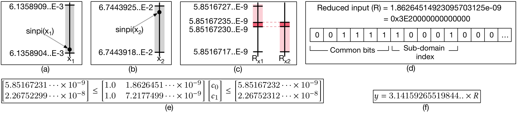
We show the correctly rounded result of for these inputs with a black circle in Figure 2(a) and Figure 2(b), respectively. It also shows the rounding interval in gray.
Step 2: Identifying the reduced interval for input R. Range reduction transforms input into . To produce the result for , we need to compute both and (i.e., multiple elementary functions). The result that we produce for and should allow us to produce the correct result for (i.e., produce a value within the rounding interval of input ).
To compute , we will generate piecewise polynomials for and . Two inputs and (Figure 2(a) and 2(b)) map to the same reduced input after range reduction,
Now, we need to deduce an interval for the output of and an interval for the output of such that the result of output compensation produces a value within the rounding interval for . We compute the correctly rounded value () of in double using the oracle and set it as our initial guess for (i.e., a singleton). Similarly, we compute the interval for . Now, we need to check if these intervals are sufficient to produce the correct output for the original input . Section 3.2 provides our detailed algorithm. The key idea is to simultaneously lower the lower bound for both and and check if output compensation produces the correct result for all inputs. Similarly, we deduce the upper bound for both and . The reduced interval for from the perspective of is . Similarly, the reduced interval for from the perspective of is . These reduced intervals for corresponding to and are shown in Figure 2(c). They are not identical because our approach considers the numerical error in both range reduction and output compensation.
Step 3: Splitting the reduced domain into sub-domains. Now that we have reduced intervals for all reduced inputs, the next task is to generate polynomials for and . We illustrate this process with . It is similar for . Even after range reduction, there are approximately million unique reduced inputs for . Using our counterexample guided polynomial generation strategy (Step 4), we attempt to generate a polynomial for the entire reduced domain. If we cannot generate a polynomial or the polynomial does not satisfy the performance constraints, then we split the reduced input domain into smaller sub-domains to generate piecewise polynomials. We iteratively split the domain into smaller sub-domains until we can produce a polynomial that produces the correct results for all inputs and satisfies the performance criterion.
Let us say we want to generate 32 (i.e. ) piecewise polynomials for the domain . We use the bit-pattern of the reduced input in double to identify the sub-domain. Although the domain of R is , the value of R in our reduced inputs ranges between along with . There is a large gap of values between the reduced input and . This is because we have already handled special cases for the original input. Excluding the reduced input , all other reduced inputs in the double representation have the left-most six bits identical. Hence, we use 5-bits after the six left-most bits to identify the sub-domain for the piecewise polynomial. Figure 2(d) shows the reduced input , its double bit-pattern, and the 5-bits used to identify the sub-domain.
Step 4: Generating a polynomial for a sub-domain. The final step is to produce a polynomial that approximates for a particular sub-domain. This polynomial must produce a value within the reduced interval for each reduced input in the sub-domain. This requirement can be encoded as a linear constraint for each reduced input,
where is a polynomial that approximates .
We show the generation of the polynomial for sub-domain with bit-pattern . First, we sample a portion of the reduced inputs (e.g., 2 in Figure 2(e)). Second, we encode the two reduced inputs and reduced intervals as linear constraints to create a LP query (see Figure 2(e)). Third, we use a LP solver to identify coefficients that satisfy the constraints. The generated polynomial is shown in Figure 2(f). Fourth, we check if the generated polynomial produces a value within the reduced interval for all inputs in the sub-domain. In this case, there are two reduced inputs where the generated polynomial does not produce a value within the reduced interval. Fifth, we add both counterexamples (i.e., reduced inputs) to the sample. Next, we create a LP query using these four reduced inputs and intervals. Then, we check if the generated polynomial satisfies all reduced inputs in the sub-domain corresponding to bit-pattern .
After generating polynomials for all 32 sub-domains, we store the coefficients of the piecewise polynomial in a table, which is indexed by the bit-pattern of the reduced input that identifies the sub-domain. The approximation for the elementary function is now ready. To produce the result for input , our library will perform range reduction on , identify the reduced input , identify the sub-domain based on the bit-pattern of , evaluate the piecewise polynomial using the coefficients from the table, perform output compensation, and round the result to a 32-bit float to produce the correctly rounded result.
3. Generating Piecewise Polynomials
Our goal is to generate polynomial approximations for elementary functions that produce the correctly rounded result for all inputs in 32-bit target representations . Similar to our prior work on RLibm (Lim et al. 2021; Lim et al. 2020a), we approximate the correctly rounded result rather than the real value of . We extend it in three main directions. First, we develop counterexample guided polynomial generation with sampling to make this approach feasible with 32-bit types. Second, we design techniques to generate piecewise polynomials, which provide performance improvements. Third, we develop modified range reduction techniques for a class of elementary functions and develop methods to deduce rounding intervals when range reduction involves multiple functions.
Correctly rounded result. For a given input and elementary function , the output of our approximation is the correctly rounded result if it is equal to the value of computed with real numbers and then rounded to the target representation. We use to denote the rounding function that rounds computed with real numbers to target representation . All internal computation such as range reduction, polynomial evaluation, and output compensation is performed in representation where has higher precision than . To attain good performance, is a representation that is supported in hardware (e.g., double).
Our approach. There are three main tasks in creating polynomial approximations with our approach. First, we need to create a range reduction function, which we denote as , that reduces input to a reduced input in a smaller domain. Once we have the result of the elementary function for the reduced input (let’s say ), we need to develop an output compensation function, which we denote as , to produce the result of for input . Second, we need to generate polynomial approximations for each elementary function in the reduced domain (e.g., there were two elementary functions and after range reduction in Section 2). We need to generate polynomials for each in the reduced domain when there are millions of reduced inputs in each reduced input domain. We have to ensure that the polynomials generated for each in the reduced domain produce correctly rounded results for all inputs after output compensation and polynomial evaluation is performed in . Third, we may have to split the reduced input domain to generate piecewise polynomials for each to create efficient implementations.
High-level sketch. Algorithm 1 provides a high-level sketch of our approach. Given an elementary function and a list of inputs , we compute the correctly rounded result in our target representation (line 4) and compute the rounding interval of in (lines 14-17). If our approximation of produces a value in the rounding interval, then the result will round to . Next, we compute the reduced input using range reduction. The range reduction may require us to compute multiple elementary functions to produce the result for . Hence, we identify the range of values that each function should produce such that the result when used with output compensation produces a value in the rounding interval of (line 7). We call this range of values for the reduced input as the reduced interval (see Section 3.2). Finally, we approximate each elementary function used in output compensation with piecewise polynomials of degree (line 11) with counterexample guided polynomial generation and by using an LP solver. A single polynomial for each may not be ideal for performance. To create efficient implementations, we iteratively split the domain of the reduced input into multiple sub-domains (see Section 3.3). Even such sub-domains for the reduced inputs can have millions of reduced inputs. Hence, we create a sample of the reduced inputs, generate constraints to ensure that the polynomial of degree produces a value in the reduced interval for the reduced inputs in the sample, and query the LP solver to solve for the coefficients. When the LP solver returns the coefficients, we check whether the generated polynomial produces a value within the reduced interval for all inputs in the sub-domain. We add any input that violates the constraints to the sample and repeat this process. We call this process as counterexample guided polynomial generation. At the end of this process, our approach produces piecewise polynomials for each , where the results of when used with output compensation produces the correctly rounded result for all inputs when rounded to .
3.1. Computing Rounding Intervals
Our approach approximates the correctly rounded result rather than the real value. Hence, the first step is to identify the correctly rounded result using an oracle and then identify all values in that rounds to the correct result in . As has higher precision than , there is a range of values in that our approach can produce and still round to the correctly rounded result in . We call this range the rounding interval. Algorithm 1 illustrates our steps to compute the rounding interval for each input (lines 14-17). We compute the oracle correctly rounded result, , using the MPFR math library with a large number of precision bits. To compute the rounding interval, we identify the smallest value that rounds to when rounded to and the largest value that rounds to when rounded to . This search procedure can be efficiently implemented either using a binary search or by leveraging the properties of and . As long as our approach produces a value in the rounding interval for input , it will produce the correctly rounded result.
3.2. Computing Reduced Rounding Intervals
Range reduction is crucial for any technique that generates approximations for elementary functions. It is particularly important with our approach for 32-bit types because the condition number of the LP problem increases drastically if the input domain has both extremely large and small values. Further, large inputs can cause overflows during the evaluation of a polynomial with a large degree in .
After computing rounding intervals from Algorithm 1, we have a list of constraints that our approximation for needs to satisfy for each input to produce the correctly rounded result. The range reduction and subsequent output compensation can require us to approximate multiple elementary functions . The next step is to identify reduced inputs to and a range of values that should produce such that the result of the output compensation produces a value in for each . The input to is the reduced input and the range of values that should produce is the reduced interval.
Algorithm 2 shows the steps in deducing the reduced interval. For each constraint , we can identify the reduced input by performing range reduction on (line 6). However, computing the reduced interval is challenging. We present an algorithm to deduce reduced intervals when output compensation () is monotonic (either increasing or decreasing), which is the case with all range reductions that we explore in the paper.
To compute the reduced interval, we identify all functions used in (line 4). Then, we compute the correctly rounded result for each in using an oracle (line 7). If the result of output compensation using ’s does not produce a value in the rounding interval for , then either the range reduction technique should be redesigned or the precision of should be increased.
Now, we have a candidate value (i.e., ) for each to produce the correctly rounded result of . We have to deduce the maximum amount of freedom available for each . We initially set the reduced intervals for each to be (line 10). Next, we identify if we can decrease the lower bound of the intervals of . For a given reduced input of input , we check if using the preceding values of in for all ’s with output compensation produces a value in the rounding interval of . If it does, then we widen the reduced interval by replacing each with the preceding value. We repeat the process until the result of output compensation using the preceding values no longer produces a value in (lines 12-15). This procedure to compute the lower bound can be efficiently implemented by performing binary search between and the minimum representable value.
Similarly, we identify if we can increase the upper bound of the interval for each . For each upper bound of , we identify the value that succeeds and check whether the result of output compensation using the succeeding value produces a value in . If it does, then we widen the reduced interval by replacing each with the succeeding value. We repeat the process until output compensation produces a value outside the interval of input (lines 17-20). The upper bound of the reduced interval can be efficiently computed by performing binary search between and the maximum representable value. Finally, we store the reduced constraints for each function in a list .
Each corresponding to contains reduced intervals for the reduced input to produce a correct result for input . As multiple inputs can map to the same reduced input , there can be multiple reduced constraints and for the same reduced input corresponding to original inputs and . The reduced intervals and are not exactly identical to account for numerical errors in range reduction and output compensation. Our polynomial approximation for must satisfy the constraints to produce the correctly rounded result for and to produce the correctly rounded result for . Thus, we generate a single combined interval by computing the common interval between them. If there is no common interval between all reduced intervals corresponding to the same reduced input, then it implies that there is no polynomial approximation for that produces the correctly rounded results for all inputs in the original domain. The library designer will have to redesign range reduction in such cases.
3.3. Efficient Piecewise Polynomials
After the above steps, we have a list of reduced constraints in for each reduced input and for each function that we need to approximate. The next step in our approach is to generate polynomials that approximate and satisfy the constraints in . Even after range reduction, there can be hundreds of millions of reduced inputs. The counterexample guided polynomial generation algorithm, which we describe in Section 3.4, can likely generate a single polynomial in many cases. However, it will also have a large degree and may not be efficient. To generate high performance math libraries, we propose the generation of piecewise polynomials. Effectively splitting the domain into smaller domains for the generation of piecewise polynomials is essential to improve performance. Hence, we group the reduced input into sub-domains based on the bit-patterns of the reduced input in .
Algorithm 3 describes our steps to generate piecewise polynomials. Range reduction techniques for many elementary functions can create both positive and negative reduced inputs (e.g., , , ). The bit-patterns for positive and negative reduced inputs in will not have common bits at the beginning (e.g., the explicit sign bit distinguishes positive and negative values in double). Hence, we separate the reduced inputs (and their intervals) into two groups: that contains negative reduced inputs and that contains non-negative reduced inputs (lines 2-3). We create polynomial approximations for each and (lines 4-5). This step also allows us to subsequently group the reduced input into sub-domains in an efficient manner.
If contains only negative or positive reduced inputs, we try to generate a single polynomial of degree that satisfies all reduced constraints in (line 11 and 17) using our counterexample guided polynomial generation (see Section 3.4). If it cannot generate a polynomial of degree that satisfies all constraints, then we split the reduced input domain in into multiple sub-domains (lines 9-13 in GenApproxHelper). We iteratively split the domain of reduced inputs into sub-domains based on the bit-pattern of in (i.e., SplitDomain call in line 10). To split the reduced input domain, we first identify the smallest reduced input and the largest reduced input . Then, we compute the number of consecutive bits that are identical in the bit-string representation of and in starting from the most significant bit. We use the next bits to identify the sub-domain for the piecewise polynomial. Subsequently, we group the reduced inputs and reduced intervals based on the bit-pattern of the reduced input into sub-domains ( returned by SplitDomain). We try to generate a polynomial of degree that satisfies all reduced constraints in for all ’s belonging to (lines 16-19). Using bit-patterns of the reduced input in allows us to efficiently identify the sub-domain for the piecewise polynomial with two bitwise operations (and and a shift). Once we generate a polynomial for each sub-domain of every , the coefficients of the polynomial are stored in a table, which is indexed using the bit-pattern of the reduced input for each .
3.4. Counterexample Driven Polynomial Generation
Once we have the reduced input and the reduced intervals, we structure the problem of generating polynomials as a linear programming problem similar to our prior work on RLibm (Lim et al. 2021; Lim et al. 2020a). Even after range reduction and creation of sub-domains for the generation of piecewise polynomials, we need to generate a polynomial approximation when there are several million reduced inputs and reduced intervals in the context of 32-bit types. However, they are beyond the capabilities of modern LP solvers, which can handle a few thousand constraints. To address this issue, we propose counterexample guided polynomial generation with sampling. The key insight is that we do not need to add every reduced input and interval as a constraint in the LP formulation as long as we identify and add the highly constrained intervals.
Our counterexample guided polynomial generation strategy takes as input the set of reduced constraints corresponding to reduced inputs that belong to a particular sub-domain. The goal is to generate a polynomial of degree that produces a value in the reduced interval for each reduced input . Each reduced input and the corresponding interval specifies the following linear constraint for a polynomial of degree that we want to generate:
The task of the polynomial generator is to find coefficients for the polynomial.
To scale to 32-bit types, we sample a small fraction of the reduced input and intervals. Algorithm 4 reports our counterexample guided polynomial generation process. It takes two inputs: the degree of the polynomial and the set of reduced inputs and intervals (i.e., ) for generating a polynomial approximation for an elementary function on reduced inputs for sub-domain . We maintain the reduced inputs and their intervals in increasing order. Then we uniformly sample the reduced inputs based on the distribution of reduced inputs. If there are a large number of reduced inputs in a particular region of the sub-domain, then our method has more samples from that region. We also add highly constrained reduced inputs and intervals (i.e., the correctly rounded result and the lower bound/upper bound is less than , which is set by the math library designer) to the sample.
Then we express all constraints in the sample using a single system of linear inequalities and solve for the coefficients using an LP solver (line 4). If there are points in the sample, the system of linear inequalities is of the following form:
There are two issues with the polynomial generated using the sampled reduced inputs that we need to address. First, as the LP solver returns coefficients as real numbers, the coefficients are rounded to a value in . As a result of rounding error, the result of polynomial evaluation for a particular reduced input in the sample may not lie within its rounding interval. Second, the polynomial generated using the sample may not satisfy the constraints for the entire set of reduced inputs and their corresponding intervals.
We address the real coefficients issue with a search-and-refine procedure similar to RLibm. When the LP solver returns real coefficients and we round it to , we check whether evaluating the polynomial satisfies constraints for every input in the sample. If it does not, then we select the input and reduce its rounding interval (either replace the lower bound with its succeeding value or replace the upper bound with the preceding value). Then we repeat the above process until it generates a polynomial that either satisfies all constraints in the sample when evaluated in or cannot find a polynomial of degree . If we cannot find a polynomial that satisfies all constraints in the sample, then we split the entire reduced domain in into even smaller sub-domains and repeat this process.
If we successfully generate a polynomial that satisfies all constraints in the sample, then we check whether this polynomial satisfies all constraints in (line 10-15). If satisfies all constraints, then we return the polynomial (line 7). If there is any constraint not satisfied by in the entire set of reduced inputs, then we add that reduced input and its interval to the sample (i.e., adding the counterexample in lines 12-13). We repeat the process of generating the polynomial with the new sample. If the number of constraints in the sample exceeds a threshold at any point, then we determine that we cannot generate a polynomial for the sub-domain . Our function to generate the coefficients for the polynomial (i.e., GetCoeffsUsingLP) using an LP solver generates a polynomial of a lower degree (than input degree ) if it is possible to do so.
4. Experimental Evaluation
|
|
|
|
|
|
|
|
| ||||||||||||||||||
|---|---|---|---|---|---|---|---|---|---|---|---|---|---|---|---|---|---|---|---|---|---|---|---|---|---|---|
| ✓ | ✗(4.2E5) | ✗(5) | ✗(1060) | ✗(5) | ✗(5) | N/A | N/A | |||||||||||||||||||
| ✓ | ✗(3.1E5) | ✓ | ✗(276) | ✓ | ✓ | N/A | N/A | |||||||||||||||||||
| ✓ | ✗(3.0E7) | ✗(1) | ✗(1.5E5) | ✗(1) | ✗(1) | N/A | N/A | |||||||||||||||||||
| ✓ | ✗(1.7E5) | ✓ | ✗(2.5E5) | ✓ | ✓ | ✗(5.1E8) | ✗(5.1E8) | |||||||||||||||||||
| ✓ | ✗(1.7E5) | ✗(2) | ✗(7.2E5) | ✗(2) | N/A | ✗(6.5E7) | ✗(1026) | |||||||||||||||||||
| ✓ | ✗(1.7E5) | ✓ | ✗(3.9E5) | ✓ | N/A | N/A | N/A | |||||||||||||||||||
| ✓ | ✗(7.1E7) | ✗(2) | ✗(2.5E5) | ✗(2) | ✗(2) | N/A | N/A | |||||||||||||||||||
| ✓ | ✗(1.8E7) | ✓ | ✗(1.4E5) | ✓ | ✓ | ✗(1.1E7) | ✓ | |||||||||||||||||||
| ✓ | N/A | N/A | ✗(3.4E5) | ✓ | ✓ | N/A | N/A | |||||||||||||||||||
| ✓ | N/A | N/A | ✗(3.8E5) | ✓ | ✓ | N/A | N/A |
We provide details on our prototype, experimental methodology, and the results of our experiments to check the correctness and performance of the generated functions.
4.1. Experimental Setup and Methodology
Prototype. The RLibm-32 prototype generates correctly rounded elementary functions for 32-bit floats and posit32, which is a 32-bit posit type providing tapered precision (i.e., more precision than float for values near 1) (Gustafson 2017). It contains ten correctly rounded elementary functions for 32-bit floats and eight elementary functions for the posit32 type. To generate correctly rounded elementary functions with good performance, the user can provide custom range reduction functions and specify the degree or the structure of the polynomial (i.e., odd or even). RLibm-32 uses the MPFR library (Fousse et al. 2007) with up to 400 precision bits to compute the oracle for and rounds it to the target representation, which is good enough to compute the oracle result for double (Lefèvre and Muller 2001). RLibm-32 uses SoPlex (Gleixner et al. 2012), an exact rational LP solver, for generating coefficients for the polynomials with a five minute time limit. We use a threshold of fifty thousand reduced inputs and intervals in the sample for counterexample guided polynomial generation. RLibm-32’s math library performs range reduction, polynomial evaluation, and output compensation using double precision. Polynomial evaluation uses the Horner’s method (Borwein and Erdelyi 1995). We designed novel extensions to range reduction for many elementary functions, which is inspired by table-based range reduction (Tang 1989; Tang 1990; Tang 1991; Daramy-Loirat et al. 2006). The appendix provides additional details about range reduction for each elementary function. RLibm-32 is open source and publicly available (Lim and Nagarakatte 2021).
Methodology. We test the elementary functions in RLibm-32 on two dimensions: (1) ability to generate correct results and (2) performance in comparison to state-of-the-art libraries. We compare RLibm-32’s functions with four libraries: Intel’s libm, glibc’s libm, CR-LIBM (Daramy-Loirat et al. 2006), and Metalibm (Kupriianova and Lauter 2014). To use double precision libraries, we convert the float input into double, use the double function, and round the result back to float. Among these libraries, CR-LIBM has correctly rounded functions for double precision. However, CR-LIBM does not produce correctly rounded results for 32-bit floats due to double rounding. There are no math libraries available for posit32. All posit32 values can be exactly represented in double. Hence, we compare our posit32 library with glibc and Intel’s double libm and CR-LIBM.
Experimental setup. We performed all our experiments on a 2.10GHz Intel Xeon Gold 6230R machine with 187GB of RAM running Ubuntu 18.04. We disabled Intel turbo boost and hyper-threading to minimize noise. We compiled RLibm-32’s math library at the O3 optimization level. We used Intel’s libm from the oneAPI Toolkit and glibc’s libm from glibc-2.33. We generated Metalibm implementations with optimizations for AVX2 extensions enabled. Our test harness that compares glibc’s libm, CR-LIBM, and Metalibm with RLibm-32 is built using the gcc-10 compiler with -O3 -static -frounding-math -fsignaling-nans flags. To use Intel’s libm, we have to use the Intel compiler. Hence, the test harness that compares Intel libm with RLibm-32 is built using the icc compiler with -O3 -no-ftz -fp-model strict -static to obtain as many correct results as possible. Further, the size of the executable generated by statically linking RLibm-32 is 2% smaller on average when compared to the executable generated with Intel’s double libm.
Measuring performance. To compare performance, we measure the number of cycles taken to compute the result for each input using hardware performance counters. The total time taken is computed as the sum of the time taken by all inputs (i.e., all inputs for a 32-bit representation). We ran the measurements for all inputs for each function six times. Then, we compute the average time taken to compute each elementary function. As Intel’s compiler performs vectorization by default at the O3 optimization level, our above setup does not measure improvements due to vectorization. Hence, we created another test harness that creates an array of 1024 floats (i.e., inputs), populates it with different inputs, and measures the number of cycles taken to compute the results of inputs using hardware performance counters. We repeat this experiment times to compute the result and measure the total time taken for all inputs.
4.2. Generation of Correctly Rounded Results
Table 1 reports the results of our experiments to check the correctness of various elementary functions in RLibm-32 and other mainstream libraries. RLibm-32 produces the correctly rounded results for all inputs for the ten elementary functions for 32-bit floats. In contrast, elementary functions in glibc, Intel, and MetaLibm’s float library do not produce the correct result for all inputs. Multiple functions in glibc and MetaLibm’s float library produce wrong results for several million inputs. Intel’s libm also produces wrong results with several thousand inputs with the float version. When we use double precision version of functions from glibc, Intel’s libm, and CR-LIBM, it does not produce the correct result for , , , and . These cases occur when the real value of is extremely close to the rounding boundary of a floating point value. Even with a smaller mini-max approximation error in the double library compared to their float versions, these libraries do not produce the correctly rounded result for all inputs. CR-LIBM, which is a correctly rounded double library, produces wrong results for float functions due to double rounding. We observed that functions in MetaLibm do not produce correct results even when it internally uses Sollya (Chevillard et al. 2010), which can be used to generate correctly rounded implementations.
|
|
|
|
| ||||||||||
|---|---|---|---|---|---|---|---|---|---|---|---|---|---|---|
| ✓ | ✗(22) | ✗(22) | ✗(22) | |||||||||||
| ✓ | ✗(19) | ✗(18) | ✗(18) | |||||||||||
| ✓ | ✗(26) | ✗(23) | ✗(23) | |||||||||||
| ✓ | ✗(4.4E8) | ✗(4.4E8) | ✗(4.4E8) | |||||||||||
| ✓ | ✗(4.0E8) | ✗(4.0E8) | N/A | |||||||||||
| ✓ | ✗(5.2E8) | ✗(5.2E8) | N/A | |||||||||||
| ✓ | ✗(4.4E8) | ✗(4.4E8) | ✗(4.4E8) | |||||||||||
| ✓ | ✗(4.4E8) | ✗(4.4E8) | ✗(4.4E8) |
Table 2 reports that RLibm-32 produces correctly rounded results with all inputs for the eight posit32 functions. All posit32 values are representable in double precision but they cannot be represented in 32-bit floats. Hence, we use CR-LIBM, Intel and glibc’s double library to compare with RLibm-32. These libraries for double precision do not produce correct results for all posit32 inputs. Unlike functions for 32-bit floats, they produce wrong results for several million inputs especially for exponential and hyperbolic functions. One of the key reasons for wrong results is the absence of overflows to and underflows to 0 with the posit32 type. Instead, extremely large values are rounded to the largest representable value. Similarly, extremely small values are rounded to the smallest non-zero representable value in the posit32 type.
|
|
|
|
| |||||||||||
| float functions | |||||||||||||||
| 7.2E6 | 3 | 3 | |||||||||||||
| 7.2E6 | 3 | 3 | |||||||||||||
| 7.2E6 | 3 | 3 | |||||||||||||
| 5.2E8 |
|
|
| ||||||||||||
| 3.0E8 |
|
|
| ||||||||||||
| 5.2E8 |
|
|
| ||||||||||||
| 1.5E8 | 5 | 3 | |||||||||||||
| 1.5E8 | 4 | 3 | |||||||||||||
| 1.2E8 | 1 | 5 | 3 | ||||||||||||
| 1.2E8 | 1 | 4 | 3 | ||||||||||||
| posit32 functions | |||||||||||||||
| 264 | 1.1E8 | 4 | 4 | ||||||||||||
| 288 | 1.1E8 | 4 | 4 | ||||||||||||
| 685 | 1.1E8 | 3 | 3 | ||||||||||||
| 1089 | 3.5E9 |
|
|
| |||||||||||
| 814 | 7.9E8 |
|
|
| |||||||||||
| 1528 | 3.4E9 |
|
|
| |||||||||||
| 461 | 1.6E9 |
|
|
| |||||||||||
| 528 | 1.7E9 |
|
|
| |||||||||||
Piecewise polynomials generated by RLibm-32. Table 3 provides details on the piecewise polynomials generated by RLibm-32. Our goal is to get the best possible performance within a given storage budget for piecewise polynomials (i.e., number of sub-domains when we split the range of reduced inputs). Hence, we used the RLibm-32 to generate piecewise polynomials such that the degree of each polynomial was less than or equal to 8 and the number of sub-domains was less than or equal to . The output compensation for , , , and involves two elementary functions. We generate two piecewise polynomials for each of those elementary functions. There are both positive and negative reduced inputs for , , and . Hence, we created two piecewise polynomials: one for the negative reduced inputs and another for positive reduced inputs. Notably, we were able to generate a single polynomial of degree 5 and 4 that satisfies all reduced constraints for and , respectively. Both and have close to 120 million reduced inputs. Our counterexample driven polynomial generation with sampling was instrumental in creating this efficient polynomial.
Time taken to generate RLibm-32 functions. Table 3 also reports the time taken to generate the 32-bit float and the posit32 functions in RLibm-32. It ranges from 19 minutes for for the float type to approximately 25 hours for for the posit32 type. Majority of the total time total time is spent in computing the oracle result and the rounding interval using the MPFR library (i.e., 86% of total time for 32-bit floats and 55% of total time for the posit32 type). In contrast, counterexample guided polynomial generation takes 14% and 45% of the total time for 32-bit floats and the posit32 type, respectively. We noticed that it takes significantly longer to generate posit32 functions. There are fewer special cases, which requires longer oracle computation. Further, RLibm-32 generates larger piecewise polynomials for posit32 functions to account for higher precision than a 32-bit float and saturating behavior with extremal values.


4.3. Performance Evaluation of RLibm-32
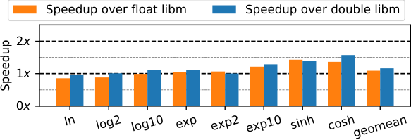
Performance of float functions. Figure 3(a) presents the speedup of RLibm-32’s float functions over glibc’s float functions (left bar in each cluster) and double functions (right bar in each cluster). On average, RLibm-32’s float functions have speedup over glibc’s float libm and speedup over glibc’s double libm. Figure 3(b) reports the speedup of RLibm-32’s float functions over Intel’s float libm and double libm. RLibm-32’s float functions have an average of speedup over Intel’s float functions and speedup over Intel’s double functions. Figure 3(c) reports that RLibm-32’s functions are on average faster than CR-LIBM functions. Figure 3(d) reports the speedup of RLibm-32’s functions over MetaLibm’s float and double functions. RLibm-32’s functions are on average and faster than MetaLibm’s float and double functions, respectively. RLibm-32’s functions are faster than all the corresponding functions in Intel libm, CR-LIBM, and MetaLibm. RLibm-32’s functions are faster than glibc’s functions except for , , and for float and for double. However, glibc’s libm produces a large number of wrong results for them. RLibm-32’s functions are not only faster but also produce correctly rounded results for all inputs.


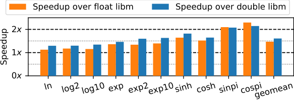
Performance of posit32 functions. The graphs in Figure 4(a), Figure 4(b), and Figure 4(c) report the speedup of RLibm-32’s posit32 functions when compared to math libraries created by re-purposing glibc’s, Intel’s, and CR-LIBM’s double functions, respectively. On average, RLibm-32’s posit32 functions are , , and faster than glibc’s libm, Intel’s libm, and CR-LIBM, respectively. All three re-purposed math libraries produce wrong results for some inputs. RLibm-32 provides the first correctly rounded functions for the posit32 type.
Vectorization. Intel compiler uses vector instructions to improve performance by default. In our experiments with vectorization using an array of 1024 inputs (see Section 4.1), RLibm-32 is on average 10% and 5% slower than Intel’s float libm and double libm, respectively. However, Intel’s compiler produces wrong results for several million inputs (without -no-ftz -fp-model strict flags). In contrast, RLibm-32’s functions are almost as fast as vectorized code while producing correct results for all inputs.

Performance impact of piecewise polynomials. To analyze the performance benefits due to piecewise polynomials, we identified elementary functions for which we could generate a single polynomial that produces correctly rounded results for all inputs (, , , and ) . We measured the change in performance with an increase in the number of sub-domains ranging from (i.e., a single polynomial) to . Figure 5 reports the performance of and with an increase in the number of sub-domains when compared to the performance of a single polynomial. We validated that all these polynomials produce the correct result for all inputs. Figure 5 does not report and because the single polynomial has the best performance. Initially, there is a small decrease in performance by moving from a single polynomial to a piecewise polynomial because the degree of the piecewise polynomial does not decrease significantly to subsume the overhead of table lookup. On increasing the number of sub-domains, we observed almost speedup with piecewise polynomials having sub-domains. It requires 6KB for storing coefficients of piecewise polynomials.
5. Case Study with for Float
We describe the case study with to illustrate the importance of carefully designing range reduction to avoid cancellation errors in output compensation. The elementary function is defined for .
Special cases. There are three kinds of special cases:
All float values are integers. Hence, for even integers and for odd integer inputs.
Range reduction of . After excluding special cases, there are more than 600 million float inputs that need to be approximated. Similar to range reduction for (Section 2.1), we use periodicity and trigonometric identities of to reduce inputs to a smaller domain. We transform input into where is an integer and . Due to periodicity, . Next, we decompose into where is the integral part of () and is the fractional part. Then, can be computed with,
To further reduce the range of , we use the fact that between is a mirror image of between with the opposite sign. We decompose into and where
We have . After reducing the input to , there are around 107 million inputs. Thus, we further reduce to a value in . We split where is an integer in the set and is a fractional value in . One possible method to compute is to use the trigonometric identity ,
The above formula is not monotonic and can have cancellation errors if (if , then ).
Creating monotonic output compensation. If , we transform and to and such that to create a monotonic output compensation function:
Then, we can compute using the trigonometric identity as follows,
This output compensation is monotonic and does not experience cancellation error. The values of ranges from to and . The computation can be computed exactly with float or double type for all values of that corresponds to . There are approximately 40 million values of . We precompute the values for and in lookup tables (i.e., 514 values in total). We create polynomial approximations for and for the reduced input domain . Using RLibm-32, we were able to generate a single degree odd polynomial for and a single degree even polynomial for . Finally, we can compute the result for with the output compensation function,
where , , and . These polynomials combined with the output compensation functions produce correctly rounded results for all inputs for and .
6. Related Work
Multiple decades of seminal work has advanced the state-of-the-art on creating approximations for FP representations (Jeannerod et al. 2011; Bui and Tahar 1999; Ziv 1991; Fousse et al. 2007; Muller 2005; Trefethen 2012; Remes 1934; De Caro et al. 2017). Further, seminal research on range reduction has made such approximation feasible (Tang 1990; Tang 1991; Tang 1989; Story and Ping Tak Peter Tang 1999; Cody and Waite 1980; Boldo et al. 2009). Simultaneously, there are verification efforts to prove bounds for math libraries (Harrison 2009; Harrison 1997a; Harrison 1997b; Sawada 2002; Lee et al. 2017), identify numerical errors with expressions that can be used in the implementation of math libraries (Chowdhary et al. 2020; Benz et al. 2012; Fu and Su 2019; Goubault 2001; Sanchez-Stern et al. 2018), and repair individual outputs of math libraries (Panchekha et al. 2015; Yi et al. 2019; Zou et al. 2019).
Correctly rounded libraries. Numerous groups have developed correctly rounded elementary functions (Jeannerod et al. 2011; Bui and Tahar 1999). Some correctly rounded libraries for FP are IBM LibUltim (Ziv 1991), Sun Microsystem’s LibMCR, CR-LIBM (Daramy-Loirat et al. 2006), MPFR math library (Fousse et al. 2007), and RLIBM (Lim et al. 2021; Lim et al. 2020a). CR-LIBM is a correctly rounded double library developed using Sollya (Chevillard et al. 2010), which generates mini-max polynomials to approximate elementary functions (Brisebarre et al. 2006; Brisebarre and Chevillard 2007). Sollya uses the modified Remez algorithm (Remes 1934) using lattice basis reduction and also computes the error bound of the polynomial (Chevillard and Lauter 2007; Chevillard et al. 2011; Melquiond 2019). Metalibm (Kupriianova and Lauter 2014; Brunie et al. 2015) builds on Sollya and generates efficient mini-max polynomials with user-defined error bounds. It also uses domain splitting and hardware specific optimizations (Kupriianova and Lauter 2015). Compared to mini-max approaches, our work approximates the correctly rounded result of and generates polynomials that already account for numerical error in range reduction and output compensation. Hence, it generates efficient and correctly rounded results for all inputs.
This paper extends our prior work on RLibm (Lim et al. 2021; Lim et al. 2020a) and John Gustafson’s Minefield method (Gustafson 2020), which advocate approximating the correctly rounded value rather than real value of an elementary function. Our prior work on RLibm also frames the problem of generating polynomials as an LP problem. We have used RLibm to create correctly rounded functions for 16-bit types: bfloat16 and posit16. This paper extends RLibm to handle 32-bit types with systematic counterexample guided polynomial generation, generation of piecewise polynomials to improve performance, and new techniques to deduce rounding intervals when range reduction involves multiple elementary functions.
Posit libraries. SoftPosit-Math (Leong 2019) and RLibm libraries provide correctly rounded math functions for 16-bit posits. In our prior work, we have produced approximations for a set of trigonometric functions using the CORDIC method for posit32 (Lim et al. 2020b). However, it does not produce correct results for all inputs. In this paper, we develop the first set of elementary functions that produce correctly rounded results for all inputs for 32-bit posits.
7. Conclusion and Future Directions
Mainstream math libraries have been designed and improved by numerous researchers spanning multiple decades. Yet, they fail to generate correct results for all inputs. This paper advocates approximating the correctly rounded value instead of the real value similar to our prior work on RLibm. It extends RLibm to scale to 32-bit representations: (a) counterexample guided polynomial generation with an LP solver to handle billions of inputs, (b) generation of constraints to account for multiple elementary functions in range reduction, and (c) generation of piecewise polynomials. The resulting functions produce correct results for all inputs and are also faster than existing libraries for 32-bit floats and posits.
Going forward, we plan to generate approximations for all commonly used elementary functions with 32-bit types, which we believe can be accomplished with our approach. However, it may require us to develop novel extensions to range reduction. Further, it may be necessary to perform range reduction in higher precision for some trigonometric functions such as sine and cosine that use . Beyond 32-bit types, we also plan to extend this approach to double precision. Our approach can generate a polynomial that produces the correctly rounded result for the sampled points in the double type. Validating the correctness of the result produced by a polynomial generated using our approach for all inputs in the double type is an open research problem. Our long-term goal is to enable the standards of existing and new representations to mandate correctly rounded results.
Acknowledgements.
We thank our shepherd Rahul Sharma and the PLDI reviewers for their feedback. We thank John Gustafson for his inputs on the Minefield method and the posit representation. This material is based upon work supported in part by the Sponsor National Science Foundation http://dx.doi.org/10.13039/100000001 under Grant No. Grant #1908798 and Grant No. Grant #1917897.References
- (1)
- Benz et al. (2012) Florian Benz, Andreas Hildebrandt, and Sebastian Hack. 2012. A Dynamic Program Analysis to Find Floating-point Accuracy Problems. In Proceedings of the 33rd ACM SIGPLAN Conference on Programming Language Design and Implementation (Beijing, China) (PLDI ’12). ACM, New York, NY, USA, 453–462. https://doi.org/10.1145/2345156.2254118
- Boldo et al. (2009) Sylvie Boldo, Marc Daumas, and Ren-Cang Li. 2009. Formally Verified Argument Reduction with a Fused Multiply-Add. In IEEE Transactions on Computers, Vol. 58. 1139–1145. https://doi.org/10.1109/TC.2008.216
- Borwein and Erdelyi (1995) Peter Borwein and Tamas Erdelyi. 1995. Polynomials and Polynomial Inequalities. Springer New York. https://doi.org/10.1007/978-1-4612-0793-1
- Brisebarre and Chevillard (2007) Nicolas Brisebarre and Sylvvain Chevillard. 2007. Efficient polynomial L-approximations. In 18th IEEE Symposium on Computer Arithmetic (ARITH ’07). https://doi.org/10.1109/ARITH.2007.17
- Brisebarre et al. (2006) Nicolas Brisebarre, Jean-Michel Muller, and Arnaud Tisserand. 2006. Computing Machine-Efficient Polynomial Approximations. In ACM ACM Transactions on Mathematical Software, Vol. 32. Association for Computing Machinery, New York, NY, USA, 236–256. https://doi.org/10.1145/1141885.1141890
- Brunie et al. (2015) Nicolas Brunie, Florent de Dinechin, Olga Kupriianova, and Christoph Lauter. 2015. Code Generators for Mathematical Functions. In 2015 IEEE 22nd Symposium on Computer Arithmetic. 66–73. https://doi.org/10.1109/ARITH.2015.22
- Bui and Tahar (1999) Hung Tien Bui and Sofiene Tahar. 1999. Design and synthesis of an IEEE-754 exponential function. In Engineering Solutions for the Next Millennium. 1999 IEEE Canadian Conference on Electrical and Computer Engineering, Vol. 1. 450–455 vol.1. https://doi.org/10.1109/CCECE.1999.807240
- Chevillard et al. (2011) Sylvain Chevillard, John Harrison, Mioara Joldes, and Christoph Lauter. 2011. Efficient and accurate computation of upper bounds of approximation errors. In Theoretical Computer Science, Vol. 412. https://doi.org/10.1016/j.tcs.2010.11.052
- Chevillard et al. (2010) Sylvain Chevillard, Mioara Joldes, and Christoph Lauter. 2010. Sollya: An Environment for the Development of Numerical Codes. In Mathematical Software - ICMS 2010 (Lecture Notes in Computer Science, Vol. 6327). Springer, Heidelberg, Germany, 28–31. https://doi.org/10.1007/978-3-642-15582-6_5
- Chevillard and Lauter (2007) Sylvain Chevillard and Christopher Lauter. 2007. A Certified Infinite Norm for the Implementation of Elementary Functions. In Seventh International Conference on Quality Software (QSIC 2007). 153–160. https://doi.org/10.1109/QSIC.2007.4385491
- Chowdhary et al. (2020) Sangeeta Chowdhary, Jay P. Lim, and Santosh Nagarakatte. 2020. Debugging and Detecting Numerical Errors in Computation with Posits. In 41st ACM SIGPLAN Conference on Programming Language Design and Implementation (PLDI’20). https://doi.org/10.1145/3385412.3386004
- Cody and Waite (1980) William J Cody and William M Waite. 1980. Software manual for the elementary functions. Prentice-Hall, Englewood Cliffs, NJ. https://doi.org/10.1137/1024023
- Daramy-Loirat et al. (2006) Catherine Daramy-Loirat, David Defour, Florent de Dinechin, Matthieu Gallet, Nicolas Gast, Christoph Lauter, and Jean-Michel Muller. 2006. CR-LIBM A library of correctly rounded elementary functions in double-precision. Research Report. Laboratoire de l’Informatique du Parallélisme. https://hal-ens-lyon.archives-ouvertes.fr/ensl-01529804
- De Caro et al. (2017) Davide De Caro, Ettore Napoli, Darjn Esposito, Gerardo Castellano, Nicola Petra, and Antonio G. M. Strollo. 2017. Minimizing Coefficients Wordlength for Piecewise-Polynomial Hardware Function Evaluation With Exact or Faithful Rounding. IEEE Transactions on Circuits and Systems I: Regular Papers (2017). https://doi.org/10.1109/TCSI.2016.2629850
- Fousse et al. (2007) Laurent Fousse, Guillaume Hanrot, Vincent Lefèvre, Patrick Pélissier, and Paul Zimmermann. 2007. MPFR: A Multiple-precision Binary Floating-point Library with Correct Rounding. ACM Trans. Math. Software 33, 2, Article 13 (June 2007). https://doi.org/10.1145/1236463.1236468
- Fu and Su (2019) Zhoulai Fu and Zhendong Su. 2019. Effective Floating-point Analysis via Weak-distance Minimization. In Proceedings of the 40th ACM SIGPLAN Conference on Programming Language Design and Implementation (Phoenix, AZ, USA) (PLDI 2019). ACM, New York, NY, USA, 439–452. https://doi.org/10.1145/3314221.3314632
- Gleixner et al. (2012) Ambros M. Gleixner, Daniel E. Steffy, and Kati Wolter. 2012. Improving the Accuracy of Linear Programming Solvers with Iterative Refinement. In Proceedings of the 37th International Symposium on Symbolic and Algebraic Computation (Grenoble, France) (ISSAC ’12). Association for Computing Machinery, New York, NY, USA, 187–194. https://doi.org/10.1145/2442829.2442858
- Goubault (2001) Eric Goubault. 2001. Static Analyses of the Precision of Floating-Point Operations. In Proceedings of the 8th International Symposium on Static Analysis (SAS). Springer, 234–259. https://doi.org/10.1007/3-540-47764-0_14
- Gustafson (2017) John Gustafson. 2017. Posit Arithmetic. https://posithub.org/docs/Posits4.pdf
- Gustafson (2020) John Gustafson. 2020. The Minefield Method: A Uniformly Fast Solution to the Table-Maker’s Dilemma. https://bit.ly/2ZP4kHj
- Harrison (1997a) John Harrison. 1997a. Floating point verification in HOL light: The exponential function. In Algebraic Methodology and Software Technology, Michael Johnson (Ed.). Springer Berlin Heidelberg, Berlin, Heidelberg, 246–260. https://doi.org/10.1007/BFb0000475
- Harrison (1997b) John Harrison. 1997b. Verifying the Accuracy of Polynomial Approximations in HOL. In International Conference on Theorem Proving in Higher Order Logics. https://doi.org/10.1007/BFb0028391
- Harrison (2009) John Harrison. 2009. HOL Light: An Overview. In Proceedings of the 22nd International Conference on Theorem Proving in Higher Order Logics, TPHOLs 2009 (Lecture Notes in Computer Science, Vol. 5674), Stefan Berghofer, Tobias Nipkow, Christian Urban, and Makarius Wenzel (Eds.). Springer-Verlag, Munich, Germany, 60–66. https://doi.org/10.1007/978-3-642-03359-9_4
- Jeannerod et al. (2011) Claude-Pierre Jeannerod, Hervé Knochel, Christophe Monat, and Guillaume Revy. 2011. Computing Floating-Point Square Roots via Bivariate Polynomial Evaluation. IEEE Trans. Comput. 60. https://doi.org/10.1109/TC.2010.152
- Kupriianova and Lauter (2014) Olga Kupriianova and Christoph Lauter. 2014. Metalibm: A Mathematical Functions Code Generator. In 4th International Congress on Mathematical Software. https://doi.org/10.1007/978-3-662-44199-2_106
- Kupriianova and Lauter (2015) Olga Kupriianova and Christoph Lauter. 2015. Replacing Branches by Polynomials in Vectorizable Elementary Functions. In Scientific Computing, Computer Arithmetic, and Validated Numerics, Marco Nehmeier, Jürgen Wolff von Gudenberg, and Warwick Tucker (Eds.). Springer International Publishing, Cham, 14–22. https://doi.org/10.1007/978-3-319-31769-4_2
- Lee et al. (2017) Wonyeol Lee, Rahul Sharma, and Alex Aiken. 2017. On Automatically Proving the Correctness of Math.h Implementations. Proceedings of the ACM on Programming Languages 2, POPL, Article 47 (Dec. 2017), 32 pages. https://doi.org/10.1145/3158135
- Lefèvre and Muller (2001) Vincent Lefèvre and Jean-Michel Muller. 2001. Worst Cases for Correct Rounding of the Elementary Functions in Double Precision. In 15th IEEE Symposium on Computer Arithmetic (Arith ’01). 111–118. https://doi.org/10.1109/ARITH.2001.930110
- Lefèvre et al. (1998) Vincent Lefèvre, Jean-Michel Muller, and Arnaud Tisserand. 1998. Toward correctly rounded transcendentals. IEEE Trans. Comput. 47, 11 (1998), 1235–1243. https://doi.org/10.1109/12.736435
- Leong (2019) Cerlane Leong. 2019. SoftPosit-Math. https://gitlab.com/cerlane/softposit-math
- Lim et al. (2020a) Jay P. Lim, Mridul Aanjaneya, John Gustafson, and Santosh Nagarakatte. 2020a. A Novel Approach to Generate Correctly Rounded Math Libraries for New Floating Point Representations. arXiv:2007.05344 Rutgers Department of Computer Science Technical Report DCS-TR-753.
- Lim et al. (2021) Jay P. Lim, Mridul Aanjaneya, John Gustafson, and Santosh Nagarakatte. 2021. An Approach to Generate Correctly Rounded Math Libraries for New Floating Point Variants. Proceedings of the ACM on Programming Languages 6, POPL, Article 29 (Jan. 2021), 30 pages. https://doi.org/10.1145/3434310
- Lim and Nagarakatte (2021) Jay P. Lim and Santosh Nagarakatte. 2021. RLibm-32. https://github.com/rutgers-apl/rlibm-32
- Lim et al. (2020b) Jay P. Lim, Matan Shachnai, and Santosh Nagarakatte. 2020b. Approximating Trigonometric Functions for Posits Using the CORDIC Method. In Proceedings of the 17th ACM International Conference on Computing Frontiers (Catania, Sicily, Italy) (CF ’20). Association for Computing Machinery, New York, NY, USA, 19–28. https://doi.org/10.1145/3387902.3392632
- Melquiond (2019) Guillaume Melquiond. 2019. Gappa. http://gappa.gforge.inria.fr
- Muller (2005) Jean-Michel Muller. 2005. Elementary Functions: Algorithms and Implementation. Birkhauser. https://doi.org/10.1007/978-1-4899-7983-4
- Panchekha et al. (2015) Pavel Panchekha, Alex Sanchez-Stern, James R. Wilcox, and Zachary Tatlock. 2015. Automatically Improving Accuracy for Floating Point Expressions. In Proceedings of the 36th ACM SIGPLAN Conference on Programming Language Design and Implementation, Vol. 50. Association for Computing Machinery, New York, NY, USA, 1–11. https://doi.org/10.1145/2813885.2737959
- Remes (1934) Eugene Remes. 1934. Sur un procédé convergent d’approximations successives pour déterminer les polynômes d’approximation. Comptes rendus de l’Académie des Sciences 198 (1934), 2063–2065.
- Sanchez-Stern et al. (2018) Alex Sanchez-Stern, Pavel Panchekha, Sorin Lerner, and Zachary Tatlock. 2018. Finding Root Causes of Floating Point Error. In Proceedings of the 39th ACM SIGPLAN Conference on Programming Language Design and Implementation (Philadelphia, PA, USA) (PLDI 2018). ACM, New York, NY, USA, 256–269. https://doi.org/10.1145/3296979.3192411
- Sawada (2002) Jun Sawada. 2002. Formal verification of divide and square root algorithms using series calculation. In 3rd International Workshop on the ACL2 Theorem Prover and its Applications.
- Sterbenz (1974) Pat H Sterbenz. 1974. Floating-point computation. Prentice-Hall, Englewood Cliffs, NJ.
- Story and Ping Tak Peter Tang (1999) Shane Story and Ping Tak Peter Tang. 1999. New algorithms for improved transcendental functions on IA-64. In Proceedings 14th IEEE Symposium on Computer Arithmetic. 4–11. https://doi.org/10.1109/ARITH.1999.762822
- Tang (1989) Ping-Tak Peter Tang. 1989. Table-Driven Implementation of the Exponential Function in IEEE Floating-Point Arithmetic. ACM Trans. Math. Software 15, 2 (June 1989), 144–157. https://doi.org/10.1145/63522.214389
- Tang (1990) Ping-Tak Peter Tang. 1990. Table-Driven Implementation of the Logarithm Function in IEEE Floating-Point Arithmetic. ACM Trans. Math. Software 16, 4 (Dec. 1990), 378–400. https://doi.org/10.1145/98267.98294
- Tang (1991) P. T. P. Tang. 1991. Table-lookup algorithms for elementary functions and their error analysis. In [1991] Proceedings 10th IEEE Symposium on Computer Arithmetic. 232–236. https://doi.org/10.1109/ARITH.1991.145565
- Trefethen (2012) Lloyd N. Trefethen. 2012. Approximation Theory and Approximation Practice (Other Titles in Applied Mathematics). Society for Industrial and Applied Mathematics, USA.
- Yi et al. (2019) Xin Yi, Liqian Chen, Xiaoguang Mao, and Tao Ji. 2019. Efficient Automated Repair of High Floating-Point Errors in Numerical Libraries. Proceedings of the ACM on Programming Languages 3, POPL, Article 56 (Jan. 2019), 29 pages. https://doi.org/10.1145/3290369
- Ziv (1991) Abraham Ziv. 1991. Fast Evaluation of Elementary Mathematical Functions with Correctly Rounded Last Bit. ACM Trans. Math. Software 17, 3 (Sept. 1991), 410–423. https://doi.org/10.1145/114697.116813
- Zou et al. (2019) Daming Zou, Muhan Zeng, Yingfei Xiong, Zhoulai Fu, Lu Zhang, and Zhendong Su. 2019. Detecting Floating-Point Errors via Atomic Conditions. Proceedings of the ACM on Programming Languages 4, POPL, Article 60 (Dec. 2019), 27 pages. https://doi.org/10.1145/3371128
Appendix A Details on Range Reduction used in RLibm-32
In this section, we describe the special cases, the range reduction, and the output compensation functions that we used to create the math library functions in RLibm-32. A given family of elementary functions (e.g., , , and ) uses similar approaches for range reduction. Hence, we first describe the range reduction technique we used for each family of elementary functions. In the subsequent sections, we describe the special cases and specific details on range reduction and output compensation that we used for float functions (Appendix B) and posit32 functions (Appendix C).
A.1. Logarithm Functions
We use a table-based approach (Tang 1990) to perform range reduction for functions. The range reduction is generally applicable to any value of . To reduce the input to the reduced input in a smaller domain, we first transform input into where is an integer representing the exponent of and is the significand. Then, can be computed with,
Next, we further reduce the range of by transforming into where , is a value in the set , and is the remaining value. Intuitively, F is the value represented by the first 8 bits of the significand and is the value represented by the rest of the bits. Then, can be computed with,
We can denote . Then, can be computed as,
The reduced input is in the range of . The computation can be efficiently performed by computing if the value can be computed ahead of time. Thus, we pre-compute the values for (128 values for each ) and (128 values in total) in lookup tables. We approximate for the reduced input domain . Finally, we can compute the result of with the output compensation function,
A.2. Exponential Functions
We also use a table-based approach (Tang 1989) to perform range reduction for functions. The range reduction is applicable for different values of . To reduce the input we first transform into where is an integer, is a value in a set and . Intuitively, represents the integral part of the value . The value represents the first 6 fractional bits of . Lastly, represents the remaining value, .
The scaling by allows us to create efficient output compensation formula. The value of can be computed using the property and as,
Multiplication by can be computed efficiently using bit-wise operations. We pre-compute and store the value of in a table (i.e. 64 values in total) and we approximate for the input domain of .
A.3. Sinpi(x)
The range reduction technique for first leverages the periodicity of to reduce the input and then use a table-based range reduction (Tang 1991) to further reduce the input. First, we transform input into where is an integer and . Then, . Next, we decompose into where is the integral part of and is the fractional part. Then, can be computed with,
Third, we use the fact that between is a mirror image of values between and decompose into,
Then, can be computed with .
We further reduce to a value between using table-based range reduction. We split into where is an integer in the set and is a real value in . The value of can be computed using the trigonometric identity :
We pre-compute and store the values of and in lookup tables (i.e. 512 values). We approximate and for the reduced input domain . Finally, we can approximate using the output compensation function,
A.4. Cospi(x)
Similar to , we leverage the periodicity of and table-based range reduction (Tang 1991) to reduce the input. Additionally, we apply some modifications to create monotonic output compensation function. First, we transform the input into where is an integer and . Due to periodicity, . Second, we decompose into where is the integral part of j and is the fractional part. Then, can be computed with,
Third, we reduce using the fact that between is a mirror image of between with the opposite sign. We decompose into and where:
Then, can be computed with .
We further reduce to a value between using table-based range reduction. We transform into and using,
where is an integer value in the set and is a fractional value in . Then, can be computed with the trigonometric identity ,
where and . This formula is monotonic for all inputs . We pre-compute and store the values of and in lookup tables (i.e. 514 values). We approximate and for the reduced input domain .
Finally, we compute the result of with the output compensation formula,
where .
A.5. Sinh(x)
We use the range reduction technique similar to the table-based range reduction technique used in CR_LIBM. First, the function has a property, . Thus, the result of for can be derived by computing .
Next, we decompose into three parts:
where both and are integers, , , and is a value in . As we will show later, scaling by allows us to compute and efficiently with minimal amount of error. If we denote and , then can be computed using the hyperbolic identities, and :
We store the values of , , , and in lookup tables. Storing and requires a total of 128 values. The number of values to store for and depends on the target representation. In the case of float, the values of does not exceed because for all non-special-case inputs. Thus, we store values for and .
Alternatively, we can choose to not store the values of and by computing and manually using the following properties,
Then, and can be computed as follows,
Although and cannot be exactly represented by double type for all , the correctly rounded value of and can be computed efficiently using integer arithmetic, floating point subtraction, and addition. We plan to incorporate this logic in our implementation of to reduced the size of the lookup table.
We approximate and for the reduced inputs . Finally, can be computed with the output compensation function,
where is the sign of .
A.6. Cosh(x)
The range reduction technique for uses a similar technique as (described in Appendix A.5) to reduce the input . Then it uses the hyperbolic identities of to perform output compensation. First, the function has a property, . Thus, the result of for can be derived by computing .
Next, we decompose into three parts similar to how we decompose the input for :
Both and are integers, , , and is a real number value in . If we denote and , then can be computed using the hyperbolic identities, and :
We store the values of , , , and in lookup tables (i.e. 388 values). We approximate and for the reduced inputs . Finally, can be computed with the output compensation function,
Appendix B Details on 32-bit Float Functions
In this section, we explain the 32-bit float functions in RLibm-32. We describe the special cases and any specific details on the range reduction technique used for each function.
B.1.
The elementary function is defined over the input domain . There are four classes of special case inputs:
We use the range reduction technique described in Appendix A.1 to decompose into , , and . In the case of , the output compensation can be mathematically computed as,
To evaluate the output compensation function in double, we store the correctly rounded value of in double. We order the operations in the following way,
This reduces the amount of numerical error for the inputs where the magnitude of is large. After range reduction, there were roughly 7.2 million reduced inputs. The reduced inputs are in the range of . We created an approximation of using RLibm-32 to generate a piecewise polynomial with polynomials of degree 3.
B.2.
The elementary function is defined over the input domain . There are four classes of special case inputs:
We use the range reduction technique described in Appendix A.1 to decompose into , , and . In the case of , the output compensation can be mathematically computed as,
To evaluate the output compensation function in double, we order the operations in the following way,
This reduces the amount of numerical error for the inputs where the magnitude of is large. After range reduction, there were roughly 7.2 million reduced inputs. The reduced inputs are in the range of . We created an approximation of using RLibm-32 to generate a piecewise polynomial with polynomials of degree 3.
B.3.
The elementary function is defined over the input domain . There are four classes of special case inputs:
We use the range reduction technique described in Appendix A.1 to decompose into , , and . In the case of , the output compensation can be mathematically computed as,
To generate efficient piecewise polynomial approximation, we store the value of in two double values, and such that is a correctly rounded value of with 106 precision bits (each double value has 53 precision bits). The value stores the higher 53 precision bits and stores the lower 53 precision bits. Then, we evaluate the output compensation function in double with the following order of operation:
This reduces the amount of numerical error for the inputs where the magnitude of is large. After range reduction, there were roughly 7.2 million reduced inputs. The reduced inputs are in the range of . We created an approximation of using RLibm-32 to generate a piecewise polynomial with polynomials of degree 3.
B.4.
The function is defined over the input domain . There are 4 classes of special case inputs:
We use the range reduction technique described in Appendix A.2 to perform range reduction and output compensation. After range reduction, there are roughly 520 million reduced inputs in the domain . We created an approximation function for negative values of reduced inputs and an approximation function for positive values of reduced inputs to efficiently split the reduced input domain. Using RLibm-32, we generated a piecewise polynomial with polynomials of degree 4 for negative reduced inputs and a piecewise polynomial with polynomials of degree 4 for positive reduced inputs.
B.5.
The function is defined over the input domain . There are 4 classes of special case inputs:
We use the range reduction technique described in Appendix A.2 to perform range reduction and output compensation. After range reduction, there are roughly 303 million reduced inputs in the domain . We created an approximation function for negative values of reduced inputs and an approximation function for positive values of reduced inputs to efficiently split the reduced input domain. Using RLibm-32, we generated a piecewise polynomial with polynomials of degree 4 for negative reduced inputs and a piecewise polynomial with polynomials of degree 4 for positive reduced inputs.
B.6.
The function is defined over the input domain . There are 4 classes of special case inputs:
We use the range reduction technique described in Appendix A.2 to perform range reduction and output compensation. After range reduction, there are roughly 521 million reduced inputs in the domain . We created an approximation function for negative values of reduced inputs and an approximation function for positive values of reduced inputs to efficiently split the reduced input domain. Using RLibm-32, we generated a piecewise polynomial with polynomials of degree 4 for negative reduced inputs and a piecewise polynomial with polynomials of degree 3 for positive reduced inputs.
B.7.
The function is defined over the input domain . There are three classes of special cases:
We use the range reduction technique described in Appendix A.3 and evaluate the range reduction and output compensation in double. After range reduction, there were roughly 117 million reduced inputs in the domain . The output compensation function for uses both and . Similarly, the output compensation function for uses the approximation of both and . Thus, we generated an approximation function for and an approximation function for that can be used to compute both and . Using RLibm-32, we created a single polynomial of degree 5 for and a single polynomial of degree 4 for .
B.8.
The function is defined over the input domain . There are three classes of special cases:
We use the range reduction technique described in Appendix A.4. We evaluate the range reduction and output compensation in double. After range reduction, there were roughly 40 million reduced inputs in the domain . The output compensation function for uses both and . These approximation functions are also used in . Thus, we generated approximation functions for and that can be used to compute the results for both and . Using RLibm-32, we created a single polynomial of degree 5 for and a single polynomial of degree 4 for .
B.9.
The function is defined over the input domain . There are four classes of special cases:
We use the range reduction technique described in Appendix A.5 and evaluate the range reduction and output compensation functions in double. After range reduction, there were roughly 147 million reduced inputs in the domain . Because the output compensation function for both and uses approximations of and , we generated a piecewise polynomial for and a piecewise polynomial for that can be used to compute both and correctly. Using RLibm-32, we created a piecewise polynomial with polynomials of degree 5 for and a piecewise polynomial with polynomials of degree 4 for .
B.10.
The functions is defined over the input domain . There are three classes of special cases:
We use the range reduction technique described in Appendix A.6 and evaluate the range reduction and output compensation functions in double. After range reduction, there were roughly 151 million reduced inputs in the domain. We approximate and for the reduced inputs in the domain . Since the output compensation function of also uses approximations of and , we generate a piecewise polynomial for and a piecewise polynomial for that can be used for the output compensation of both and . Using RLibm-32, we created a piecewise polynomial with polynomials of degree 5 for and a piecewise polynomial with polynomials of degree 4 for .
Appendix C 32-bit Posit32 Functions
In this section, we explain the 32-bit posit (posit32) functions in RLibm-32. We describe the special cases and any specific details on the range reduction technique used for each function.
C.1.
The elementary function is defined over the input domain . There are two classes of special case inputs of for posit32:
We use the range reduction technique described in Appendix A.1 to decompose into , , and . In the case of , the output compensation can be mathematically computed as,
To compute accurately, we store the value of in two double values, and , such that stores the correctly rounded value of with 106 precision bits (double type has 53 precision bits). The value stores the higher 53 precision bits and stores the lower 53 precision bits. We evaluate the output compensation function in double with the following order,
This reduces the amount of numerical error for the inputs where the magnitude of is large. After range reduction, there were roughly 115 million reduced inputs. The reduced inputs are in the range of . We created an approximation of using RLibm-32 to generate a piecewise polynomial with polynomials of degree 4.
C.2.
The elementary function is defined over the input domain . There are two classes of special case inputs of for posit32:
We use the range reduction technique described in Appendix A.1 to decompose into , , and . The output compensation function for can be mathematically computed as,
The output compensation function that we use for experiences cancellation error when for small values of . In such cases, , , and . The numerical error caused by cancellation error in the output compensation function of for posit32 poses a challenge in generating piecewise polynomials of reasonable degree and size that satisfies all reduced input and interval constraints.
Thus, we evaluate the output compensation function in double with the following order of operations,
This order subtracts two values with largest difference in magnitude, before subtracting two values with similar magnitude. After range reduction, there were roughly 115 million reduced inputs. The reduced inputs are in the range of . We created an approximation of using RLibm-32 to generate a piecewise polynomial with polynomials of degree 4. Comparatively, when we generated a piecewise polynomial for the output compensation function that evaluates in the following order,
RLibm-32 generated a piecewise polynomial with polynomials of degree 4. In all other cases of for float or posit32, adding , then adding at the end did not produce piecewise polynomial with smaller number of polynomials.
C.3.
The elementary function is defined over the input domain . There are two classes of special case inputs of for posit32:
We use the range reduction technique described in Appendix A.1 to decompose into , , and . The output compensation function of can be mathematically computed as,
To compute accurately, we store in two double values, and . The sum , if evaluated in real numbers, is the correctly rounded value of with 106 precision bits. The value stores the higher 53 precision bits and stores the lower 53 precision bits. We evaluate the output compensation function in double in the following order,
After range reduction, there were roughly 115 million reduced inputs. The reduced inputs are in the range of . We created an approximation of using RLibm-32 to generate a piecewise polynomial with polynomials of degree 4.
C.4.
The function is defined over the input domain . There are 4 classes of special case inputs:
We use a range reduction technique similar to the technique described in Appendix A.2 to perform range reduction and output compensation. More specifically, we split into segments instead of segments:
where is an integer, is a value in a set and .
Then, the output compensation formula is adjusted accordingly:
We pre-compute and store the value of in a table (i.e. 128 values in total) and approximate for the input domain of .
After range reduction, there are roughly 3.5 billion reduced inputs in the domain . We created an approximation function for negative values of reduced inputs and an approximation function for positive values of reduced inputs to efficiently split the reduced input domain. Using RLibm-32, we generated a piecewise polynomial with polynomials of degree 3 for negative reduced inputs and a piecewise polynomial with polynomials of degree 3 for positive reduced inputs.
C.5.
The function is defined over the input domain . There are 4 classes of special case inputs:
We use the range reduction technique described in Appendix A.2 to perform range reduction and output compensation. After range reduction, there are roughly 790 million reduced inputs in the domain . We created an approximation function for negative values of reduced inputs and an approximation function for positive values of reduced inputs to efficiently split the reduced input domain. Using RLibm-32, we generated a piecewise polynomial with polynomials of degree 3 for negative reduced inputs and a piecewise polynomial with polynomials of degree 3 for positive reduced inputs.
C.6.
The function is defined over the input domain . There are 4 classes of special case inputs:
We use the range reduction technique described in Appendix A.2 to perform range reduction and output compensation. After range reduction, there are roughly 3.4 billion reduced inputs in the domain . We created an approximation function for negative values of reduced inputs and an approximation function for positive values of reduced inputs to efficiently split the reduced input domain. Using RLibm-32, we generated a piecewise polynomial with polynomials of degree 3 for negative reduced inputs and a piecewise polynomial with polynomials of degree 3 for positive reduced inputs.
C.7.
The function is defined over the input domain . There are four classes of special cases:
We use the range reduction technique described in Appendix A.5 and evaluate the range reduction and output compensation functions in double. After range reduction, there were roughly 1.6 billion reduced inputs in the domain . Because the output compensation function for uses approximations of and , we generated a piecewise polynomial for and a piecewise polynomial for . Using RLibm-32, we created a piecewise polynomial with polynomials of degree 5 for and a piecewise polynomial with polynomials of degree 4 for .
C.8.
The functions is defined over the input domain . There are three classes of special cases:
We use the range reduction technique described in Appendix A.6 and evaluate the range reduction and output compensation functions in double. After range reduction, there were roughly 1.7 billion reduced inputs in the domain. We approximate and for the reduced inputs in the domain . Since the output compensation function of uses approximations of and , we generate a piecewise polynomial for and a piecewise polynomial for . Using RLibm-32, we created a piecewise polynomial with polynomials of degree 3 for and a piecewise polynomial with polynomials of degree 6 for .