Stickiness in generic low-dimensional Hamiltonian systems: A recurrence time statistics approach
Abstract
We analyze the structure and stickiness in the chaotic components of generic Hamiltonian systems with divided phase space. Following the method proposed recently in (Lozej, Robnik, Phys. Rev. E 98, 022220 (2018)), the sticky regions are identified using the statistics of recurrence times of a single chaotic orbit into cells dividing the phase space into a grid. We perform extensive numerical studies of three example systems: the Chirikov standard map, the family of Robnik billiards and the family of lemon billiards. The filling of the cells is compared to the random model of chaotic diffusion, introduced in (Robnik et al. J. Phys. A: Math. Gen. 30, L803 (1997)) for the description of transport in the phase spaces of ergodic systems. The model is based on the assumption of completely uncorrelated cell visits because of the strongly chaotic dynamics of the orbit and the distribution of recurrence times is exponential. In generic systems the stickiness induces correlations in the cell visits. The distribution of recurrence times exhibits a separation of time scales because of the dynamical trapping. We model the recurrence time distributions to cells inside sticky areas as a mixture of exponential distributions with different decay times. We introduce the variable , which is the ratio between the standard deviation and the mean of the recurrence times as a measure of stickiness. We use to globally assess the distributions of recurrence times. We find that in the bulk of the chaotic sea , while in areas of stickiness. We present the results in the form of animated grayscale plots of the variable in the largest chaotic component for the three example systems, included as supplemental material to this paper.
I Introduction
In generic Hamiltonian systems the phase space is divided into several invariant components, with regular motion on some and chaotic motion on others (Lichtenberg and Lieberman 1992). These kinds of systems are usually called mixed-type or systems with divided phase space. The exact border between the chaotic sea(s) and the regular components is hard to determine because of the typically infinite hierarchy of islands of stability embedded in the chaotic sea. The chaotic sea constitutes what is known as a "fat fractal" (Umberger and Farmer 1985). In systems with dimension two or lower invariant tori strictly separate the regular and chaotic components. In higher dimensions an invariant torus cannot strictly separate the phase space, making the analysis even more complicated. Even in the two-dimensional case very few systems where the border between the regular an chaotic parts can be exactly determined are known. Examples are the mushroom billiards introduced by Bunimovich (Bunimowich 2001) and the peiecewise linear symplectic maps (Wojtkowski 1981; Wojtkowski 1982; Malovrh and Prosen 2002; Altmann et al. 2006). However, these examples have the drawback of having only a small number of specially constructed islands of stability, in contrast to typical Hamiltonian systems, where an infinite island-around-island structure is usually present. Recently, a way of approximating a generic system with divided phase was proposed (Bunimovich et al. 2019) in order to facilitate a more rigorous analysis. The generic system is approximated by a sequence of systems with a finite number of islands that are sub-islands of the initial system. The approach was demonstrated for a class of two-dimensional billiards. The intricacies of transport in generic Hamiltonian systems remain a long standing open problem.
In systems with divided phase space, transport in the chaotic component is strongly influenced by the various structures embedded in it. A recent review of the theory of transport is given in Ref. (Meiss 2015). These systems commonly exhibit the phenomenon known as stickiness (Contopoulos 1971; Shirts and Reinhardt 1982). A good introduction to the topic of stickiness is provided by Refs. (Contopoulos and Harsoula 2010a) and (Bunimovich and Vela-Arevalo 2012). It is common for chaotic orbits to stick to islands of stability for extended periods of time. This is due to the presence of cantori, which are invariant cantor sets surrounding the islands of stability that may remain after invariant curves are broken by perturbation (Percival 1979; MacKay et al. 1984a; MacKay et al. 1984b). A chaotic orbit with an initial condition near the last invariant curve of an island of stability may become trapped in the region bounded by the cantorus for an arbitrarily long time before finally exiting through one of the holes in the cantorus into the larger chaotic sea (see Refs. (Contopoulos and Harsoula 2010a; Contopoulos and Harsoula 2010b) for a detailed description). This produces long periods of intermittent quasi-regular motion in the chaotic orbit and results in only weakly chaotic dynamics in the chaotic component in the sense of slow (power law) decay of correlations (Zaslavsky 2002) and power law tails in recurrence time distributions. The finite time dynamics of such systems thus influences the long time transport properties.
The prevalence and universality of algebraic decays in recurrence time distributions has been a matter of intense investigation over many years (Karney 1983; Chirikov and Shepelyansky 1984; Hanson et al. 1985; Meiss and Ott 1986; Zaslavsky and Edelman 2000; Weiss et al. 2003; Altmann et al. 2005; Altmann et al. 2006; Cristadoro and Ketzmerick 2008; Venegeroles 2009; Ceder and Agam 2013; Abud and de Carvalho 2013). Most theoretical results are based on the Markov tree model (Hanson et al. 1985; Meiss and Ott 1986; Cristadoro and Ketzmerick 2008; Venegeroles 2009; Ceder and Agam 2013), which predicts a power law asymptotic decay of the recurrence time distribution in generic Hamiltonian systems, taking into account the hierarchical structure of the phase space. Various numerical and theoretical studies report different values for the decay exponent ranging from 1 to 3 (a collection of the results is given in Ref. (Venegeroles 2009)). A possible explanation is that the transition to the asymptotic regime may take an arbitrarily long time and is thus very hard to observe in numerical experiments. The existence of power law decays is also very hard to prove numerically (Clauset et al. 2009) as data over many orders of magnitude is needed and fluctuations often obscured by fluctuations. One must also stress, that a divided phase space is not a prerequisite for stickiness and slow decay of correlations. Stickiness may also be produced by zero measure invariant sets like families of marginally unstable periodic orbits (MUPO) that are present also in ergodic systems (see Ref. (Bunimovich and Vela-Arevalo 2012) for a discussion). A famous example is the stadium billiard (Bunimovich 1979) where two sticky sets of MUPO are present (the so-called bouncing ball and boundary glancing orbits) that produce power law decay of correlations (Vivaldi et al. 1983).
Stickiness may be characterized in terms of various observables. Some examples include escape times from a given region in the phase space (Contopoulos and Harsoula 2010a; Bunimovich et al. 2019), finite time Lyapunov exponents (Szezech Jr et al. 2005), recurrence plots (Zou et al. 2007), recurrence time statistics (Altmann et al. 2004; Altmann et al. 2006; Abud and de Carvalho 2013) and rotation number (Santos et al. 2019). In a recent paper (Lozej and Robnik 2018) we analyzed the structure of the chaotic components of a single parameter family of billiards introduced in (Robnik 1983). The phase space was divided into a grid of cells and dynamics of the cell filling analyzed in terms of the so-called random model of diffusion in chaotic components (Robnik et al. 1997; Prosen and Robnik 1998; Robnik et al. 1999). Stickiness around islands of stability caused a slowing of the cell filling compared to the expectation from the random model. The statistics of cell recurrence times was studied and the standard deviation of the recurrence time used to identify sticky areas in the chaotic component. In this paper we use this approach to analyze the stickiness in the largest chaotic component of several examples of generic Hamiltonian systems. The three systems considered in this paper are the Chirikov standard map (Chirikov 1971), the above mentioned family of billiards and the family of lemon billiards (Heller and Tomsovic 1993).
The paper is organized as follows. In Sec. II we present the method of analyzing the stickiness in the chaotic component in terms of recurrence times on a grid of cells dividing the phase space. We introduce the random model of diffusion in chaotic components and discuss its implications on the statistics of recurrence times. we discuss the relationships between recurrence times escape times and transit times. We introduce the hyperexponential distribution to model the distributions of recurrence times in sticky areas. We introduce the variable that is the ratio between the standard deviations and the mean of the recurrence times as a means of identifying stickiness. In Sec. III we apply the method to the standard map and calculate the size of the largest chaotic component and analyze the stickiness of the various embedded structures for a large range of parameter values. In Sec. IV we do the same for two families of billiard systems, the Robnik billiards and the lemon billiards. In Sec. V we discuss the results and draw our conclusions. The supplemental material of this paper contains animations of the phase spaces of the studied systems. The animations show in terms of the variable how the structure and stickiness of the largest chaotic component changes as a function of the parameter.
II The random model and cell recurrence times
In this paper we use the moments of the distribution of recurrence times to identify sticky areas in the chaotic component, following the approach proposed in our recent paper (Lozej and Robnik 2018). The approach is based on the random model of diffusion in chaotic components, first introduced in Ref. (Robnik et al. 1997) as a model of transport in ergodic chaotic systems and extended in Refs. (Prosen and Robnik 1998; Robnik et al. 1999) for systems with divided phase space and systems with several weakly coupled ergodic sub-components. The main idea of our approach is to use a single chaotic orbit to generate the recurrence time data. The benefit is that no prior knowledge of the structure of the phase space is needed, only a single initial condition for the chaotic orbit. The idea of mapping the chaotic component by using a single chaotic orbit was used already by Umberger and Farmer (Umberger and Farmer 1985). The procedure is as follows. Let be the phase space (surface of section), the mapping and the invariant measure of our discrete dynamical system and . We divide into a grid of rectangular cells. We select a single initial condition in the chaotic component and iterate the orbit times. At each iteration the orbit visits one of the cells. We will refer to cells that are visited by the orbit at least once as filled cells and those that are never visited as empty cells. Eventually the chaotic orbit will explore all of the available phase space and the filled cells will cover the chaotic component . The empty cells belong to other invariant components.
The random model assumes that in strongly chaotic systems the cell visits are completely uncorrelated, independent from previous cell visits, they constitute a Poisson process. With this assumption the proportion of filled cells at time (number of iterations) follows the exponential law
| (1) |
where is the measure of the chaotic component and is the number of cells available to the chaotic orbit. This exponential law was first derived only for ergodic systems where and has been shown to excellently describe real data (see Ref. (Robnik et al. 1997) for details). In systems with divided phase space the basic assumption of uncorrelated cell visits does not hold in general. If the system exhibits stickiness the cell visits within the sticky areas become correlated. As we shall see in the numerical examples the cell filling is slowed by stickiness. If there are no sticky areas the cell filling is well described by Eq. (1) even in systems with divided phase space.
To quantify the effects of stickiness we measure the recurrence times in each of the cells visited by the chaotic orbit. Let for instance one of the cells. The first recurrence time to for a point is defined as the number of iterations an orbit needs to return to the same cell for the first time,
| (2) |
We are interested in the probability distributions of recurrence times
| (3) |
and its moments to the cells dividing the phase space. The idea of using the mean recurrence time to probe the size of the accessible area was first given by Meiss in Ref. (Meiss 1997) together with several results concerning the relationships between the transit, exit and recurrence times. In ergodic components the mean recurrence time is given by the Kac lemma (Kac 1959) which states
| (4) |
where the angled brackets denote the phase space average over and is the subset of the phase space accessible to orbits starting from . Taking one of the cells in the chaotic component as , its accessible set is the chaotic component and the mean recurrence time to the cell is equal to . In numerical experiments the measured mean recurrence times are distributed normally around the theoretical mean because of finite sample size effects (see Ref. (Lozej and Robnik 2018) for details). Additionally, if we assume the premise of the random model that the cell visits are completely uncorrelated (a Poisson process), the probability that a cell is visited after any number of iterations is equal, resulting in an exponential probability density function of recurrence times
| (5) |
to each individual cell. This is the result we expect in systems with strong mixing properties (Hirata et al. 1999). A common way of describing the recurrence time distributions is also in terms of the survival function or complementary cumulative distribution i. e. the probability that the recurrence time is greater than , referred to as the Poincaré recurrence time distribution by some authors (Chirikov and Shepelyansky 1984; Chirikov and Shepelyansky 1999). In the Poissonian case
| (6) |
However, the assumption of uncorrelated cell visits does not hold for areas of stickiness. If the cell is located inside an area of stickiness, the orbit is likely to visit the same cell again before escaping into the grater chaotic sea because of the dynamical trapping. As a consequence the recurrences when the orbit leaves the sticky area may happen on a vastly different time scale then when it stays inside for the entire period of recurrence. The strength of the trapping inside the sticky area may be quantified by the escape time. Let us again consider a subset of the phase space. The exit set of is the set of all points that exit after one iteration . Similarly the entry set is the set of all points that enter in one iteration . The union of the exit and entry sets is called a turnstile. The escape time is the time needed for an orbit starting in to leave
| (7) |
Analogously the entry time is the time needed to enter the set from outside
| (8) |
Orbits starting in the exit set will escape after one iteration and . Similarly orbits starting within but not in will recur to after one iteration meaning the recurrence time is . The time to transit an area is . The recurrence time to is essentially the transit time of the accessible area . The above relations as well as many other useful results are derived in Refs. (Meiss 1997; Meiss 2015). Let us now consider the recurrence times to a cell embedded inside a sticky area. The orbit starts from inside the cell and must first escape through the exit set of the cell. Then the orbit is trapped inside the sticky area for the duration of the typical escape time. The orbit may visit the cell before escaping. The rate at which this happens on average depends on the measure of the sticky area and the measure of the entry set of the cell. The orbit may also escape the sticky region before returning to the cell. The escape times from sticky areas are again related to the measures of the sticky area and its exit set. The flux trough the bordering cantori may in some cases be estimated analytically using transport theory (MacKay et al. 1984a; MacKay et al. 1984a; Meiss 2015). The orbit then spends a typical transition time in the larger chaotic sea. Depending on the structure of the phase space the orbit may also visit other sticky areas each with its own typical entry and escape times. After transitioning back to the original sticky area the orbit may again return to the cell. The typical time scales for the different possible transitions may vary greatly. We may thus expect to see several typical time scales in the recurrence time distributions to the cells inside the sticky regions.
Probing the distribution of recurrence times can only be feasibly done in a few selected cells. Our previous numerical results (Lozej and Robnik 2018) as well as those presented in this paper show that the distributions of recurrence times do indeed follow the exponential law (6) in the bulk of the chaotic sea, far away from any islands. On the other hand the distributions in cells located in the sticky areas exhibit a short time peak followed by an exponential tail. Similar results have been found by Altmann et. al. (Altmann et al. 2004) in one dimensional chaotic maps. We propose to model the separation of time scales introduced by the trapping inside sticky regions with a mixture of exponential distributions with different time scales (known also as the hyperexponential distribution). We model the survival function as
| (9) |
where are the mixture coefficients and and are dimensionless parameters characterizing the relevant time scales in terms of the mean recurrence time . The mean and variance of the distribution (9) are given by
| (10) | ||||
| (11) |
For a global understanding of the distributions of recurrence times their moments can be calculated for all cells iteratively with each orbit visit. In cells where the distribution of recurrence times is exponential (6), the standard deviation is equal to its mean . Due to the Kac lemma the mean recurrence time is also in sticky cells, giving the relation for the parameters of distribution (9). If the number of exponential components is the standard deviation is increased (Papadopolous et al. 1993). The variable (the coefficient of variation) is thus very useful for identifying sticky cells. In areas of the chaotic component with strong chaos and no stickiness , indicating an exponential distribution of recurrence times, while indicates stickiness. The larger the value of the stronger the stickiness. However, a comment must be made in regard to the convergence of at infinite times. In our model we only take into account exponentially decaying distributions. Other types of distributions may also be applicable. Of particular interest are recurrence time distributions with algebraic decays. The variable would diverge if the distribution of recurrence times exhibits sufficiently strong power law tails. If asymptotically the distribution decays as , the second moment diverges if . In the numerical case this would mean that the value of would keep increasing with the number of orbit iterations. This may limit the applicability of the variable in the infinite time limit, but would still provide valuable information about the stickiness for finite times. We note that when comparing results for the exponents with other papers one must take care as some authors use and others as the observed distribution.
III Results for the standard map
The Chirikov standard map (Chirikov 1971) is one of the most well studied 2D area-preserving mappings and is applicable to many areas of physics (for a review see Ref. (Chirikov and Shepelyansky 2008)). The mapping is given by
| (12) | |||
where we consider the variables on a torus , taking both variables and the prime symbol denoting the variables after one map iteration. The parameter controls the degree of chaos in the system. In Fig. 1 we show how the overall size of the largest chaotic component changes with the parameter value. This is calculated by counting the number of filled cells after mappings. The chaotic component is a "fat fractal" (Umberger and Farmer 1985) making an accurate estimate for its area difficult. In the infinite time limit the filled cells cover the chaotic sea. Naturally, the cells on the border of the chaotic sea must partially cover also the other invariant components. Taking all of the area of the filled cells as belonging to the chaotic component thus overestimates its true area. In the worst case the border cells barely touch the chaotic component and in reality barely contribute to the real area of the chaotic sea and thus counting them as filled overestimates the true area of the chaotic component. In the numerical data we define a border cell as one that has at least one empty neighbour. By this definition all features that are smaller than one cell, like for instance tiny islands of stability, are missed. The maximum error for the (lower bound of the area) is estimated by taking the border cells as empty. The area changes relatively smoothly with the parameter value but not monotonically, with many oscillations when the various islands are destroyed.
Below the critical value invariant curves limit transport in the direction and the phase space features several separate chaotic components of significant size. At the critical value (Greene 1979; MacKay 1983) the chaotic components merge into a single one where the variable can take all values. At this value the so called golden invariant circles are broken. However, for cantori, that remain after the last invariant curve is destroyed, may severely impede transport from one part of the chaotic component to the other. This may very clearly be seen in the cell filling curves using the procedure described in Sec. II. In Fig. 2 we show the cell filling for three values of . The cell filling closely follows the random model prediction at where the phase space is practically entirely filled by one chaotic component and no islands are visible. In the other cases the cell filling is slowed and distinct step-like features appear. The steps signify that the orbit is confined in some area of phase space for some time before eventually finding its way through one of the holes in the cantorus. The increase in the number of visited cells is therefore halted for the duration of the trapping. The size of the steps gives an indication of the relative sizes of the areas of phase space separated by the cantori. Similar large steps in the cell filling at were found also by Meiss in Ref. (Meiss 1994) because of the trapping of the orbits by the golden cantorus.
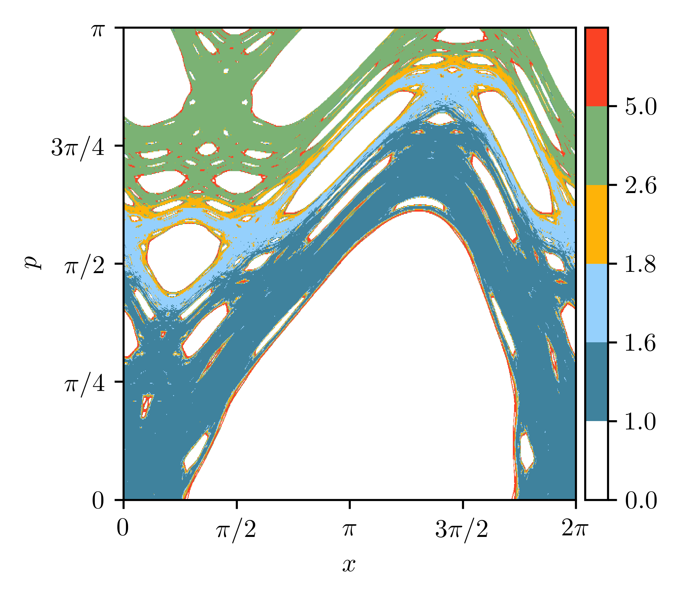
The areas of stickiness may be found by examining the cell recurrence times in the chaotic component. In Fig. 3 we show a color plot of on a grid of cells for the largest chaotic component of the standard mapping at , right above the critical value. The values of and are determined numerically at mappings for each visited cell. Similar results are obtained if the value for the mean is calculated from the numerically determined using the formula instead. The white areas belong to other invariant components, mostly islands of stability. Several large distinct areas of uniform values of are visible. They stratify the phase space in the direction. In the largest one (dark blue) , followed by (light blue), a thin layer with and in the second largest (green). Areas of stickiness may also be seen around several of the islands of stability with (red) usually increasing in several stages. Each change in color signifies a strong barrier (cantorus with small holes) that is present between the two adjacent areas. By examining the phase portrait for right below the critical value and comparing it to the plot at we see that the border between the green and yellow areas is very near the last spanning invariant curve (the golden invariant circle) before its destruction (not shown). The cantorus left in its place at causes the trapping of the orbit in one area or the other. The value of may be used to quantify the relative strength of the stickiness when comparing the different sticky areas.
In Fig. 4 we show gray-scale plots of on a grid of cells. In the following we shall refer to this type of plot as an -plot. In panel (a) we show again the plot for the largest chaotic component of the standard mapping for . On panel (b) the S-plot at is shown. Comparing the two we see that the phase space at is no longer stratified in the direction. The holes in the cantori have grown large enough as to no longer impede the transport and most of the chaotic component is covered by cells with indicating a nearly perfect exponential distribution of recurrence times. The largest sticky area, with in this case is formed around the large island around the stable stationary point , . This is responsible for the small step in the cell filling for as seen in Fig. 2. Thin sticky areas may also be seen around many of the small islands.
The survival functions of recurrence times in three selected cells are presented in the lower panels of Fig. 4. The positions of the cells in the phase space are shown as labeled (colored in online version) dots in panels (a) and (b). In panel (c) we show the survival function at in the three distinct areas with different values of described above. The first cell (blue) is located in the large sub-component with . The second in the thin layer with . The third cell (red) is located in the upper sub-component . The three survival functions are shown also in the log-log plot in panel (d). The survival functions can effectively be modeled using the hyperexponential distribution (9). The fitting procedure is done using a version of Prony’s method (Feldmann and Whitt 1997) and goes as follows. At large enough values of only the exponential with the slowest decay rate significantly contributes to the survival function. We select a cutoff point at some large enough value and consider only the tail of the survival function. We fit the tail with a single exponential function . We then subtract from the data to eliminate this contribution. We repeat the process until the desired number of time scales is reached. We used up to four exponential functions to fit the data. The parameters are given in table 1. Using the distribution parameters in formulas (10) and (11) we obtain results consistent with the values of taken from the S-plots. In table 1 and the the log-log plots on panel (d) we may clearly see that the time scales of recurrences are significantly separated in the sticky cells. The short time recurrences must be associated with orbits that do not leave the sticky area before revisiting the cell. The other time scales are probably related with the orbit sticking to other substructures and transitions between them through the chaotic sea. To be able to determine the parameters analytically a thorough understanding of the structure of the sticky sets and the associated turnstiles would be needed and is in general very difficult. At the survival functions in all three cells are exponential (panel (e)) with decay rate .
| Cell 1 | ||||
|---|---|---|---|---|
| 0.380 | 1.55 | 53.0 | n/a | |
| 0.18 | 0.80 | 0.02 | 0 | |
| Cell 2 | ||||
| 0.326 | 2.01 | 105 | 1210 | |
| 0.29 | 0.04 | 0.59 | 0.10 | |
| Cell 3 | ||||
| 0.112 | 3.69 | 10.2 | 142 | |
| 0.09 | 0.46 | 0.40 | 0.036 | |

The numerical stability of the value of in the three cells is analyzed in Fig. 5. In panel (a) we show the -plot at , and . Comparing this with the plot at in Fig. 4 (a) we see the results are qualitatively the same but the values of are lower in sticky cells than they were at . Cells with greater stickiness still exhibit higher values of . In non-sticky cells regardless of the grid size. In panels (b) and (c) we plot the value of as a function of the number of iterations for two orbits one with the initial condition and the other . We compare the results for the two orbits at different grid sizes. Panel (b) shows the results at and panel (c) at . After a transient regime the value of stabilizes and both orbits give similar results. The transient is more pronounced in cell 3 and the fluctuations are larger as the orbits need to cross the strong barriers of the golden cantori to reach this region. The distributions of recurrence times are therefore quite stable after the transient regime.

Because of the fractal nature of the chaotic sea decreasing the cell size at any scale, resolves more of the underlying structure of the phase space. Typically, new islands will appear with additional sticky sub-structures. In Fig. 6 we show the survival functions in the three cells at different grid sizes (a) , (b) and (c) . The parameters of the fitted corresponding hyperexponential distributions are given in table 1 for , table 2 for and table 3 for . The survival functions are not independent of the grid size. While the general shape can be described using the hyperexponential distribution the parameters change when making the cell smaller essentially sampling the distribution in a sub-cell of the larger cell. The time scales represented in the survival functions of the smaller cells are generally of the same order of magnitude as in the larger cell occasionally varying up to a factor of ten (compare the values of each cell at different cell sizes in the tables). The mixing coefficients may, however change significantly when the cell size is changed. Usually one or two of the exponential functions are dominant with the others contributing only a few percent to the mixture. The scaling of with regard to the grid size is depicted on panel (e). The scaling is not algebraic but is still monotonous and the hierarchy of stickiness is maintained (regions with larger at some grid size have larger values of at different grid sizes as well).
In Ref. (Meiss 1994) Meiss uses the density of orbit visits to show how orbits tend to accumulate around sticky objects for extended periods of time. The paper includes a color plot similar to the -plots. In our experience using the variable instead of the density gives more stable results both in terms of taking different initial conditions as well as in terms of the number of iterations. The results when using densities can also be somewhat asymmetric for long times (the densities near the sticky islands at positive are not the same as those around the equivalent islands at negative ) whereas the -plots produce very symmetric results (as can be seen in the animations contained in the supplemental material). The characteristic times in the standard map, including recurrence times, have recently been analyzed by Harsoula et. al. (Harsoula et al. 2019), where they observed similar distributions of recurrence times to small boxes. They have found exponential distributions in the large chaotic component before and after the critical value of and distributions with long power law tails in the small chaotic components that are separated below the critical value. The difference in their approach is that they select multiple initial conditions inside the box, which may contain also regular initial conditions. In our approach no "contamination" of the results due to the presence of regular trajectories may occur.
| Cell 1 | ||||
|---|---|---|---|---|
| 0.111 | 1.38 | 32.7 | n/a | |
| 0.03 | 0.92 | 0.05 | 0 | |
| Cell 2 | ||||
| 0.100 | 11.9 | 95.8 | 544 | |
| 0.10 | 0.09 | 0.59 | 0.22 | |
| Cell 3 | ||||
| 0.0355 | 1.94 | 8.12 | 162 | |
| 0.03 | 0.18 | 0.71 | 0.07 | |
| Cell 1 | ||||
|---|---|---|---|---|
| 0.791 | 2.23 | 53.1 | n/a | |
| 0.67 | 0.32 | 0.01 | 0 | |
| Cell 2 | ||||
| 0.609 | 1.2 | 162 | 1480 | |
| 0.56 | 0.09 | 0.30 | 0.05 | |
| Cell 3 | ||||
| 0.349 | 6.97 | 89.2 | n/a | |
| 0.32 | 0.64 | 0.35 | 0 | |
The supplemental material (Sup) of this paper includes an animation of the plots as the value of the nonlinearity parameter changes from to in steps of . For each parameter value is computed for each cell in the grid, with and the results are compiled into an animation. In the animation we can observe how the various invariant curves are destroyed, leaving behind cantori producing sticky areas around islands of stability. The stickiness is most pronounced (the value of is largest) right after the destruction of the invariant curve as the holes in the cantorus are very small and consequently the flux through it is small as well. When the chaotic orbit penetrates the area bounded by the cantorus it is trapped between it and the next invariant curve that survived the perturbation. As the nonlinearity parameter is increased the holes in the cantorus grow larger, the flux increases, until eventually the cantorus loses its ability to impede transport and the sticky area disappears. In the beginning of the animation () we see the successive breaking of the invariant tori. In fact it is still very hard to pinpoint the exact point at which the torus breaks as the orbit may need a very large number of iterations to find its way through one of the holes of the cantorus. If the number of numerical iterations is shorter we may sometimes miss the exact point of the breaking of the torus. The occasional flickering (a portion of the chaotic component disappears for a few frames of the animation) of the outer most areas (in the direction) of the chaotic component is a consequence of this effect. We also see an overall increase of even in the middle of the chaotic sea at the points where chaotic components of significant sizes merge with the large chaotic sea, either when a spanning invariant curve, like the golden invariant circle or one of the large islands breaks apart. This is very noticeable at small values of because the overall relative size of the chaotic sea is small and comparable with the sizes of the other chaotic components before the merger. The times for the transitions between the different weakly coupled areas may be very large. At the time an orbit needs for the transition into the upper part of the phase space may be larger than iterations. In Ref. (MacKay et al. 1984b) the authors give formula for the average transit time trough the golden cantorus , which gives an estimate of at . The same scaling law holds for any so called boundary circle.
IV Results for billiard systems
The other example we provide in this paper are two families of dynamical billiards. A billiard is a dynamical system which consists of a free moving particle confined inside a closed domain in Euclidean space referred to as the billiard table. The billiard tables presented in this paper will all be two dimensional . The particle moves freely inside the billiard table in straight lines and is specularly reflected when hitting the edge of the table, meaning the angle of reflection is equal to the angle of incidence. The dynamics can be described as a mapping that gives the position on the boundary and the velocity of the particle at each successive collision. As the energy of the particle is conserved the speed can be fixed to without loss of generality. The phase space can be described by the Poincaré-Birkhoff coordinates , where is the arc-length of the billiard boundary and the conjugated momentum is the sine of the reflection angle of the particle . The phase space is thus a cylinder , where we take to be periodic with a period equal to the total length of the billiard boundary . The dynamics is given by a sequence of points generated by the area preserving mapping that maps one collision to the next (Berry 1981).
IV.1 The Robnik billiards
We first present the results for the family of billiards introduced by Robnik in Ref. (Robnik 1983) given as a smooth conformal mapping of the unit disk in the complex plane. In the real plane the boundary of the billiards may be given as the following curve in polar coordinates
| (13) |
where is the polar angle and is the deformation parameter. We choose the point as the origin for the arc-length coordinate . The family of billiards has been well studied both in the classical and quantum domain (Robnik 1983; Robnik 1984; Batistić and Robnik 2013; Lozej and Robnik 2018). At the boundary is a circle giving an integrable billiard. The other extreme case is the cardioid billiard which was proven to be an ergodic K-system by Markarian (Markarian 1993). In between the phase space is generally divided into chaotic components and regular components. Up to regular spanning invariant curves, known as Lazutkin tori exist because of the convex shape and the smoothness of the billiard (Lazutkin 1973). Small islands may remain up until but take up only a tiny fraction of the phase space. In Fig. 7 we show how the relative size of the largest chaotic component changes with the value of . The curve is qualitatively similar to the one for the standard map but with less pronounced oscillations. The error has been estimated in the same way as with the standard map described in the previous section.
The supplemental material (Sup) of this paper includes an animation of the -plots of the largest chaotic component starting at up to in steps of on a grid of cells taking iterations. In the animation we see the successive breaking of the invariant tori that separate the largest chaotic component (forming around the unstable period-2 orbit) and the smaller chaotic components around the higher order unstable periodic orbits, following the typical KAM like scenario. Again, as in the standard map example, we see multiple cantori affecting the transport in the direction with increasing in several layers towards the edge of the chaotic component. We may also find cases where stickiness around the islands is dominant.
In Fig. 8 the cell filling graphs for two are shown together with the random model prediction. At the numerical curve coincides with the model while in the case the numerical cell filling is slower. The steps in the curve are very shallow indicating the trapping areas are relatively small compared to the whole extent of the chaotic component. The trapping times are also very long. The final extent of the chaotic component is filled only after . The -plots corresponding to the two parameter values are portrayed in Fig. 9. In panel (a) at we see strongly sticky areas around several KAM islands as well as near the Lazutkin tori. In panel (b) at we still see some regular islands of significant size but there are no noticeable strongly sticky areas (there might be a very thin slightly sticky area around the largest regular islands). The recurrence time distributions are exponential virtually everywhere in the chaotic component and the motion is uncorrelated. The basic assumption in the random model is thus largely satisfied which explains agreement of the numerical cell filling with the model.

In Fig. 10 we show an example of an island, which surrounds the stable period-3 orbit, breaking because of the perturbation. We show the -plot of the same area (half of the island can be seen also in Fig. 9(a)) at increasing values of the parameter. In panel (a) the island is still intact and surrounded by a thin sticky layer and the typical structure of ever smaller islands around islands of higher order resonances. In panel (b) the island has broken into a five island structure. The area between the islands is filled by the chaotic component and is very sticky because of the cantorus left behind the recently destroyed invariant curve. In panel (c) the area between the islands is already far less sticky as the holes in the cantorus have grown larger. We see thin layers of greater stickiness around the four flanking islands. In panel (d) the stickiness is almost gone, with only traces remaining. In all four images we can observe tiny islands of stability around the main islands. Some of the islands are smaller than the resolution of the cell grid. If the cell is not entirely filled by the chaotic component the probability of hitting the cell is smaller. This changes the distribution of recurrence times to the cell and as a consequence . The -plot is thus also a good way of detecting tiny islands of stability.

IV.2 The lemon billiards
Finally we present the results in the family of billiards known as the lemon billiards introduced by Heller and Tomsovic in Ref. (Heller and Tomsovic 1993) and further studied together with some generalizations in the classical and quantum domain by many authors (Lopac et al. 1999; Makino et al. 2001; Lopac et al. 2001; Chen et al. 2013; Bunimowich et al. 2015). The lemon billiard tables are formed by the intersection of two circles of equal radius (we set without loss of generality) with the distance between their centers being less than their diameters . The billiard boundary in the real plane may be given by the following implicit equations
| (14) | ||||
We choose the point as the origin for the arc-length coordinate . In contrast to the Robnik billiards the boundary of the lemon billiards is never smooth as a kink is formed where the two circular arcs meet. Because of this there are no Lazutkin tori. The period-2 orbit connecting the points at the middle of the two circular arcs, and , is stable for all values of with the exception of where it is only marginally stable. In this case this orbit is part of a whole one-dimensional family of marginally unstable periodic orbits (MUPO). It is easy to see that at any orbit starting from the middle of the circle will hit the other circle perpendicularly and retrace its path, because the centers of one circle exactly overlaps the arc of the other. The phase space of the lemon billiards is thus of the mixed-type for all values of with the possible exception of , where it might be ergodic. Our numerical results were not able to verify this as a tiny island, that the chaotic orbit was unable to penetrate, remained even for iterations. In Fig. 11 we show how the area of the largest chaotic component changes with the value of . The curve bears no resemblance with the previous examples exhibiting extremely non monotonic behavior. Because of the small overall size and the large proportion of cells bordering regular components the error of the estimate is very large for .
An animation of the -plots of the largest chaotic component for the lemon billiards is included in the supplemental material (Sup). The parameter changes from to in steps of . The grid size is cells and we take iterations. At the billiard shape is very close to a circle. Only initial conditions that hit the boundary close to the kink where the two circles meet generate chaotic motion. This results in a very regular web like structure of the chaotic component and the embedded KAM islands. The structure can be related to initial conditions that hit the kink after 1, 2, 3… iterations. When is increased, more and more of the periodic orbits lose stability (although there is a tendency for them to re-stabilize) sometimes leaving behind interesting sticky structures. The structure of the chaotic components changes radically with the value of and many interesting special cases may be found - we present a selection of them in Fig. 12. In panel (a) we see the -plot at . Only a few islands of stability may be seen none of which exhibit any stickiness, with in all cells belonging to the chaotic sea. At , panel (b), the major islands of stability around the stable period-2 orbit are not sticky, while the the island structures around the stable period-4 orbit are. In panel (c) we show the special case where the sticky family of MUPOs can be observed. The value of increases roughly exponentially in the sticky area as we get closer to the MUPO in the star like structure. An exponential increase of stickiness as one gets closer to the sticky object has been described by Contopoulos and Harsoula in terms of escape times in Ref. (Contopoulos and Harsoula 2010a). Similar star like structures have been observed by Chen et. al. (Chen et al. 2013) in ergodic generalizations of the lemon billiards. A tiny island is still visible in the middle but we expect this to also be filled if the orbit is iterated for long enough. For the period-2 orbit is again stable and an island is formed around it. In panel (d) we show the -plot at . Only one island of stability is visible and it is not sticky. Many other interesting examples may be found in the animation in the supplemental material. The examples with finitely many islands of stability may prove interesting for more rigorous analytical treatment. In Fig. 13 the corresponding cell filling graphs are shown. We see that the cell filling is influenced by the sticky islands . In the other three cases the cell filling is close to the random model prediction. We see that non-sticky islands even of substantial sizes like in the cases of and do not induce correlation in the cell visits. The MUPOs in the case also have an almost negligible effect even though we see stickiness in the -plot. This might be because the sticky area is very small compared to the size of the chaotic sea.

One of the largest sticky areas in this billiard family may be found at . The size of sticky area is approximately . In Fig. 14 we show (panel (a)) the cell filling for two different orbits, the first started with an initial condition outside the sticky area and the second inside the sticky area, as well as the corresponding -plot (panel (b)). The -plot is the same for both initial conditions. Outside the sticky area which is above the expected for the exponential distribution of recurrence times. This is similar to the result in the standard map slightly above the critical value of the nonlinearity parameter. Inside the sticky area the value of quickly increases and then plateaus at about . The increase is roughly exponential but is hard to determine exactly as the border of the sticky area is riddled by islands of stability. The orbit starting from outside the sticky area (blue) needs a little less than iterations to penetrate inside while the orbit starting from the inside (red) needs a little less than to escape. The escape time is thus much shorter than the entry time to the sticky area. The shape of the steps in the two cell filling curves are reminiscent of two periods of exponential filling of the type given by Eq. (1). With some simplification the system could be described with a two component random model in the manner of Ref. (Robnik et al. 1999).

V Conclusions and discussion
In this paper we presented a method for analyzing stickiness in chaotic components of Hamiltonian systems with divided phase space. The method is based on the examination of recurrence times of a long chaotic orbit into small cells dividing the phase space. The variable, which is the ratio between the standard deviation and the mean of recurrence times, is used to assess the distributions of recurrence times in the chaotic component. Where the distribution is exponential and the recurrences are effectively random. In sticky areas a separation of time scales between recurrences occurs due to the dynamical trapping and .
We applied the method to three example systems: the standard map, the Robnik billiards and the lemon billiards. The main conclusions are as follows: The random model of diffusion in chaotic components describes the filling of the cells well in systems with divided phase space, even when the regular components are of significant size, if there is no stickiness. Where sticky objects are present the cell filling is slowed by the cantori causing the stickiness. In the vast majority of cases in the bulk of the chaotic sea, meaning the recurrences are completely uncorrelated. The distributions of recurrence times in these areas are exponential. rapidly increases in areas of stickiness in the vicinity of sticky objects. These can be zero measure objects like sticky marginally unstable periodic orbits or more extensive object like sticky islands. The distributions of recurrence times in sticky areas may effectively be modeled using the hyperexponential distribution. When particularly strong cantori are present in the system that separate large areas of the chaotic component the value of is slightly increased even in the bulk of the chaotic sea, for instance right after the destruction of a spanning invariant torus. The two examples given in the paper where this is most visible is the standard map at and the lemon billiard at . The latter example also shows that the time to escape a sticky region is shorter than the time needed to enter the sticky region. The -plots provide an excellent overview and allow us to follow the changes in the structure of the chaotic sea as we change the parameter. In this way we may identify the positions of sticky objects as well as the extent and relative strength of the stickiness. The shape of the sticky areas bordered by cantori can be seen very clearly. Furthermore, the even tiny islands of stability that are smaller than the cells can be traced, as they still affect the recurrence time distributions. The method may therefore also be useful in providing numerical evidence of ergodicity. The statistic is stable with regards to the initial condition of the chaotic orbit and the number of iterations after a transient regime. However is not stable with regard to the grid size, which is a significant drawback. The scaling of is not algebraic but still monotonous and the -plots at different grid sizes give qualitatively identical results.
As mentioned in the introduction there has been a long standing debate about the presence and universality of algebraic decay of recurrence time distributions in Hamiltonian systems with divided phase space. Our method only distinguishes an exponential distribution from any other distribution. This might be a hyperexponential distribution as was the case in all the examples found in this paper or any other distribution including those with power law tails. However, detecting distributions with algebraic decay exponents is possible with our method, as the standard deviations for such distributions diverges. If the value of keeps increasing with the number of iterations this would be a very clear indication of such an algebraic decay. It would also be interesting to study the recurrences in specific sticky areas as a unified domain. The -plots may be used to determine the borders of the sticky area of interest and then the escape times or recurrence times to the specified domain can be studied. One of the interesting open questions is also how to quantitatively assess the effects of stickiness on the transport inside the chaotic component, especially in cases where the phase space is bounded like in billiard systems where the usual arguments using the decay of correlations (Karney 1983) have to be modified (Venegeroles 2009). The sticky areas may slow down transport at finite times considerably, leading to anomalous diffusion (Manos and Robnik 2014). As recently shown for the standard map (Harsoula and Contopoulos 2018) the transition to the asymptotic regime may be extremely long.
We used the -plots to identify several interesting cases in the lemon billiard with apparently finitely many islands of stability and no stickiness as well as cases with extreme stickiness. Such special cases might lend themselves to more rigorous mathematical analysis paving the way to a more general understanding of the transport in mixed type systems in the generic case, which is a long standing open problem. The special cases in the lemon billiards may also prove interesting for analysis in the quantum domain as the spectral statistics and localization of eigenstates in the semiclassical limit are closely linked to the transport properties of the classical system (Batistić et al. 2019). Research of the effects of stickiness on the localization of quantum eigenstates is currently underway.
Acknowledgments
The author acknowledges the financial support from the Slovenian Research Agency (research core funding No. P1-0306). The author would like to thank Prof. Marko Robnik for support and stimulating discussions, and careful reading of the manuscript and Dr. B. Batistić for providing the use of his excellent numerical library (Ben). The author thanks the anonymous referees for excellent critical, informative and helpful remarks.
References
- Lichtenberg and Lieberman (1992) A. J. Lichtenberg and M. A. Lieberman, Regular and Chaotic Dynamics (New York: Springer Verlag, 1992).
- Umberger and Farmer (1985) D. K. Umberger and J. D. Farmer, Physical Review Letters 55, 661 (1985).
- Bunimowich (2001) L. A. Bunimowich, Chaos 11, 802 (2001).
- Wojtkowski (1981) M. Wojtkowski, Communications in Mathematical Physics 80, 453 (1981).
- Wojtkowski (1982) M. Wojtkowski, Ergodic Theory and Dynamical Systems 2, 525 (1982).
- Malovrh and Prosen (2002) J. Malovrh and T. Prosen, J. Phys. A: Math. Gen 35, 2483 (2002).
- Altmann et al. (2006) E. G. Altmann, A. E. Motter, and H. Kantz, Physical Review E 73, 026207 (2006).
- Bunimovich et al. (2019) L. A. Bunimovich, G. Casati, T. Prosen, and G. Vidmar, Experimental Mathematics 0, 1 (2019).
- Meiss (2015) J. Meiss, Chaos: An Interdisciplinary Journal of Nonlinear Science 25, 097602 (2015).
- Contopoulos (1971) G. Contopoulos, The Astronomical Journal 76, 147 (1971).
- Shirts and Reinhardt (1982) R. B. Shirts and W. P. Reinhardt, The Journal of Chemical Physics 77, 5204 (1982).
- Contopoulos and Harsoula (2010a) G. Contopoulos and M. Harsoula, International Journal of Bifurcation and Chaos 20, 2005 (2010a).
- Bunimovich and Vela-Arevalo (2012) L. A. Bunimovich and L. V. Vela-Arevalo, Chaos: An Interdisciplinary Journal of Nonlinear Science 22, 026103 (2012).
- Percival (1979) I. C. Percival, Journal of Physics A: Mathematical and General 12, L57 (1979).
- MacKay et al. (1984a) R. S. MacKay, J. D. Meiss, and I. C. Percival, Physical Review Letters 52, 697 (1984a).
- MacKay et al. (1984b) R. S. MacKay, J. D. Meiss, and I. C. Percival, Physica D: Nonlinear Phenomena 13, 55 (1984b).
- Contopoulos and Harsoula (2010b) G. Contopoulos and M. Harsoula, Celestial Mechanics and Dynamical Astronomy 107, 77 (2010b).
- Zaslavsky (2002) G. M. Zaslavsky, Physics Reports 371, 461 (2002).
- Karney (1983) C. F. Karney, Physica D: Nonlinear Phenomena 8, 360 (1983).
- Chirikov and Shepelyansky (1984) B. V. Chirikov and D. L. Shepelyansky, Physica D: Nonlinear Phenomena 13, 395 (1984).
- Hanson et al. (1985) J. D. Hanson, J. R. Cary, and J. D. Meiss, Journal of Statistical Physics 39, 327 (1985).
- Meiss and Ott (1986) J. D. Meiss and E. Ott, Physica. D, Nonlinear Phenomena 20, 387 (1986).
- Zaslavsky and Edelman (2000) G. Zaslavsky and M. Edelman, Chaos: An Interdisciplinary Journal of Nonlinear Science 10, 135 (2000).
- Weiss et al. (2003) M. Weiss, L. Hufnagel, and R. Ketzmerick, Physical Review E 67, 046209 (2003).
- Altmann et al. (2005) E. G. Altmann, A. E. Motter, and H. Kantz, Chaos: An Interdisciplinary Journal of Nonlinear Science 15, 033105 (2005).
- Cristadoro and Ketzmerick (2008) G. Cristadoro and R. Ketzmerick, Physical Review Letters 100, 184101 (2008).
- Venegeroles (2009) R. Venegeroles, Physical Review Letters 102, 064101 (2009).
- Ceder and Agam (2013) R. Ceder and O. Agam, Physical Review E 87, 012918 (2013).
- Abud and de Carvalho (2013) C. V. Abud and R. E. de Carvalho, Physical Review E 88, 042922 (2013).
- Clauset et al. (2009) A. Clauset, C. R. Shalizi, and M. E. Newman, SIAM review 51, 661 (2009).
- Bunimovich (1979) L. A. Bunimovich, Comm. Math. Phys. 65, 295 (1979).
- Vivaldi et al. (1983) F. Vivaldi, G. Casati, and I. Guarneri, Physical Review Letters 51, 727 (1983).
- Szezech Jr et al. (2005) J. D. Szezech Jr, S. R. Lopes, and R. L. Viana, Physics Letters A 335, 394 (2005).
- Zou et al. (2007) Y. Zou, M. Thiel, M. C. Romano, and J. Kurths, Chaos: An Interdisciplinary Journal of Nonlinear Science 17, 043101 (2007).
- Altmann et al. (2004) E. G. Altmann, E. C. Da Silva, and I. L. Caldas, Chaos: An Interdisciplinary Journal of Nonlinear Science 14, 975 (2004).
- Santos et al. (2019) M. S. Santos, M. Mugnaine, J. D. Szezech Jr, A. M. Batista, I. L. Caldas, and R. L. Viana, Chaos: An Interdisciplinary Journal of Nonlinear Science 29, 043125 (2019).
- Lozej and Robnik (2018) Č. Lozej and M. Robnik, Physical Review E 98, 022220 (2018).
- Robnik (1983) M. Robnik, Journal of Physics A: Mathematical and General 16, 3971 (1983).
- Robnik et al. (1997) M. Robnik, J. Dobnikar, A. Rapisarda, T. Prosen, and M. Petkovšek, J. Phys. A: Math. Gen. 30, L803 (1997).
- Prosen and Robnik (1998) T. Prosen and M. Robnik, J. Phys. A: Math. Gen. 31, L345 (1998).
- Robnik et al. (1999) M. Robnik, T. Prosen, and J. Dobnikar, Journal of Physics A: Mathematical and General 32, 1147 (1999).
- Chirikov (1971) B. V. Chirikov, Research concerning the theory of non-linear resonance and stochasticity, Tech. Rep. (CM-P00100691, 1971).
- Heller and Tomsovic (1993) E. J. Heller and S. Tomsovic, Phys. Today 46, 38 (1993).
- Meiss (1997) J. D. Meiss, Chaos: An Interdisciplinary Journal of Nonlinear Science 7, 139 (1997).
- Kac (1959) M. Kac, Probability and Related Topics in Physical Sciences (Interscience Publishers, 1959).
- Hirata et al. (1999) M. Hirata, B. Saussol, and S. Vaienti, Communications in Mathematical Physics 206, 33 (1999).
- Chirikov and Shepelyansky (1999) B. V. Chirikov and D. L. Shepelyansky, Physical Review Letters 82, 528 (1999).
- Papadopolous et al. (1993) H. Papadopolous, C. Heavey, and J. Browne, Queueing theory in manufacturing systems analysis and design (Springer Science & Business Media, 1993).
- Chirikov and Shepelyansky (2008) B. Chirikov and D. Shepelyansky, Scholarpedia 3, 3550 (2008), revision190245.
- Greene (1979) J. M. Greene, Journal of Mathematical Physics 20, 1183 (1979).
- MacKay (1983) R. S. MacKay, Physica D: Nonlinear Phenomena 7, 283 (1983).
- Meiss (1994) J. D. Meiss, Physica D: Nonlinear Phenomena 74, 254 (1994).
- Feldmann and Whitt (1997) A. Feldmann and W. Whitt, in Proceedings of INFOCOM’97, Vol. 3 (IEEE, 1997) pp. 1096–1104.
- Harsoula et al. (2019) M. Harsoula, K. Karamanos, and G. Contopoulos, Physical Review E 99, 032203 (2019).
- (55) See Supplemental Material at [URL will be inserted by publisher] for animations of the S-plots as a function of the parameter.
- Berry (1981) M. V. Berry, Eur. J. Phys. 2, 91 (1981).
- Robnik (1984) M. Robnik, Journal of Physics A: Mathematical and General 17, 1049 (1984).
- Batistić and Robnik (2013) B. Batistić and M. Robnik, J. Phys. A: Math. Theor. 46, 315102 (2013).
- Markarian (1993) R. Markarian, Nonlinearity 6, 819 (1993).
- Lazutkin (1973) V. F. Lazutkin, Mathematics of the USSR-Izvestiya 7, 185 (1973).
- Lopac et al. (1999) V. Lopac, I. Mrkonjic, and D. Radic, Phys. Rev. E 59, 303 (1999).
- Makino et al. (2001) H. Makino, T. Harazama, and Y. Aizawa, Phys. Rev. E 63, 056203 (2001).
- Lopac et al. (2001) V. Lopac, I. Mrkonjic, and D. Radic, Phys. Rev. E 64, 016214 (2001).
- Chen et al. (2013) J. Chen, L. Mohr, H.-K. Zhang, and P. Zhang, Chaos 23, 043137 (2013).
- Bunimowich et al. (2015) L. A. Bunimowich, H.-K. Zhang, and P. Zhang, Commun. Math. Phys 341, 3781 (2015).
- Manos and Robnik (2014) T. Manos and M. Robnik, Physical Review E 89, 022905 (2014).
- Harsoula and Contopoulos (2018) M. Harsoula and G. Contopoulos, Physical Review E 97, 022215 (2018).
- Batistić et al. (2019) B. Batistić, Č. Lozej, and M. Robnik, Physical Review E 100, 062208 (2019).
- (69) Available at https://github.com/benokit/time-dep-billiards.