Absence of obvious tidal tails around the globular cluster NGC 63972020Absence of obvious tidal tails around the globular cluster NGC 6397–A.1
Abstract
In this work, we use body simulations performed on GPU to trace the past 10 Gyr dynamical history of a globular cluster (GC) similar to NGC 6397 in the tidal field of a Milky Way-like galaxy and we compare our simulated GCs with data from the third Gaia early data release. Our simulations predict, in contrast to what is deduced from the data, that such a cluster should present strong and extended tidal tails by more than 6 Gyr ago (right after the first third of its life), exceeding 1 kpc of length, and should be roughly disrupted by current time. We analyzed each of our initial conditions, such as initial mass and density parameters, as well as the dark matter shape, and we argue that the most likely reason for such discrepancy between the data and our simulations is related to the fact that we consider a purely baryonic cluster in the beginning of each model we test. We discuss that if our globular cluster was initially embedded in a dark matter minihalo, the latter could act as a protecting envelope, which prevents the tidal stripping of the luminous matter, while being itself gradually disrupted and removed in the course of the cluster evolution. This could explain why an insignificant amount of dark matter is required to describe the velocity dispersion in NGC 6397, up to at least a few half-mass radii.
Keywords:
galaxy dynamics – (Galaxy:) globular clusters: individual: NGC 6397 – Milky Way – methods: orbital integrations – body simulations1 Introduction
Globular clusters (GCs) are among the oldest known stellar systems in astrophysics. These sources are spherically shaped collections of stars, often associated with very poor metallicities and usually occupy the outer regions of their host galaxy, within its dark matter (DM) halo (see Gratton et al. 2019 for a complete review). The Milky Way (MW) itself hosts more then 150 GCs (Harris 2010), some of which occupy relatively close positions with respect to the Galaxy centre (Gaia Collaboration et al. 2018).
Although GCs might seem as simple sources at first, they are subject to various enigmas that are yet not completely understood. For example, there is no clear consensus pertaining to their formation mechanisms (e.g. Forbes & Bridges 2010): they could have been formed in smaller galaxies that later merged to become their present host galaxy (e.g. Searle & Zinn 1978, Bullock & Johnston 2005, Abadi et al. 2006 and Peñarrubia et al. 2009), as well as they could have been formed in-situ. There is also the possibility that they were formed in DM minihalos in the early Universe (Peebles & Dicke 1968; Peebles 1984b), but we do not consider this dark component in our simulations.
Moreover, GCs serve as laboratories to many astrophysical studies such as the motion and internal kinematics of spherical systems (e.g. Baumgardt et al. 2019, Vasiliev 2019), intermediate-mass black holes (Greene et al. 2019) and multiple stellar populations (Carretta et al. 2009). Therefore, it is important to understand the impact of dynamics on the long-term evolution of GCs so that one can trace back their history and better model the underlying physics of these complex sources.
In this work, we examine whether stellar dynamics is sufficient to explain the survival of the GCs under the effect of strong tidal fields of the MW over the course of their evolution via body simulations. To perform such an analysis, we model the nearby GC NGC 6397, the second closest GC to our Sun at only 2.39 kpc away (Brown et al. 2018), with a pericentre of some few kpc (1.7 – 2.9 kpc, Gaia Collaboration et al. 2018), thus undergoing considerable tidal interactions with the MW. NGC 6397 had its dynamics broadly analyzed (e.g. Heyl et al. 2012, Watkins et al. 2015a, Watkins et al. 2015b, Husser et al. 2016, Baumgardt et al. 2019 and Vitral & Mamon 2021) and was observed many times, by different space missions such as the Gaia Space Telescope (Gaia Collaboration et al. 2018) and the Hubble Space Telescope (Bellini et al. 2014).
Our body simulations performed on GPU indicate that, when assuming a purely baryonic source and a cuspy DM density for the MW, strong tidal effects should have started disrupting this cluster after the first third of its life due to the dense background of DM and stars in our Galaxy. We tested different scenarios such as the presence of a central black hole, as well as different density slopes and characteristic radii. Then, we compare our simulation results to observations from Gaia EDR3. Our paper is organized as follows: In Section 2, we describe the most recent data concerning NGC 6397 derived from observations. Section 3 provides a description of the body modelling. In Section 4, we outline details of our numerical simulations and method. In Section 5, we discuss our results and their interpretation. In Sections 6 and 7, we outline and draw our conclusions.
2 Observations of NGC 6397
Given its proximity, the dynamics of NGC 6397 was broadly observed during the course of recent years: Bellini et al. 2014 performed deep observations of the cluster’s core using the Hubble Space Telescope (HST) and provided thousands of proper motions, which were later complemented by the proper motions from the data releases of the Gaia astrometric mission (hereafter, Gaia), better probing its outskirts (Gaia Collaboration et al. 2018, Gaia Collaboration et al. 2020). In addition, line-of-sight velocities were also measured in various studies such as Husser et al. 2016 and Lovisi et al. 2012.
2.1 Dynamics
With this vast amount of velocity data, the dynamical analysis of this GC is also the subject of many studies: Heyl et al. 2012 analyzed main sequence stars along with white dwarfs from HST observations and measured a mass of M⊙ for a photometric distance of 2.53 pc (even though they estimate a kinematic distance of 2.2 kpc). They also compared the velocity dispersion and effective radii in different magnitude bins and assigned a considerable mass segregation to this GC. In addition, Husser et al. 2016 used MUSE spectrograph data to measure a mean line-of-sight (LOS) velocity of thousands of stars from this GC, to which Kamann et al. 2016 later fitted a 600 M⊙ central black hole.
More recently, Vitral & Mamon 2021 combined data from HST, Gaia DR2 and the Multi Unit Spectroscopic Explorer (MUSE) to perform a Bayesian mass-modeling analysis of this cluster through the handling of the Jeans equation. They found strong evidence for isotropy up to 8 arcmin (i.e. pc) from the cluster’s centre and used a distance of 2.39 kpc (Brown et al. 2018) to estimate a total luminous mass of M⊙. They provided important constraints on the surface density profile by modelling the inner cusp of this post core-collapse cluster with a Sérsic model (Sérsic 1963) and also found strong mass segregation by jointly modeling stellar populations with different mean mass. Finally, although this work managed to fit an intermediate-mass black hole of mass M⊙ located in this cluster’s centre, the authors ruled it out in favour of an unresolved inner sub-cluster of stellar remnants, after analyzing both the statistics and the physics involved in both scenarios.
Using the orbital radius from Gaia DR2 data (Vasiliev 2019) and the mass from Vitral & Mamon 2021, we calculate the theoretical tidal radius of NGC 6397 using the formula of Bertin & Varri 2008. All these analyses provide us with strong constraints regarding the choice of parameters in our simulations (see Table 1), and thus allow us to interpret our conclusions with better confidence.
2.2 Tails
The strong tidal field of the MW could, in principle, form extended tidal tails in NGC 6397. Leon et al. 2000 found, while looking for shock imprints, that this GC presented few over-densities (tidal tails) at larger radii, which they were not able to robustly distinguish from dust extinction and therefore classified them as unreliable measurements. Recently, Kundu et al. 2020 claimed to have identified tidal tails beyond the cluster tidal radius, which could be related to shocks and tidal disruption. Kundu et al. 2020 argue that it was beyond the scope of their work to derive a precise fit of the proper motion distribution, and that an idea of the cluster intrinsic dispersion was sufficient to select tidal stars. However, at regions distant from the cluster centre, such as the ones probed in their work, the contamination of MW field stars can be increasingly problematic, especially when targeting a small number of stars (120 tidal stars).
In a recent work, Ibata et al. 2020 performed a thorough search for stellar streams in many MW GCs and successfully identified an irregular stellar stream around NGC 6397, extending 18o on the sky, which would mean, disregarding projection effects, a tail of roughly 750 pc. In the following sections, we try to detect even more extended tidal tails in NGC 6397.
3 Numerical modelling
In this section, we comment some of the previous attempts to numerically model NGC 6397 and then present the models for the MW and NGC 6397, that provide the initial conditions for our simulations.
| NGC 6397 | Stellar mass | |
| Sérsic radius | pc | |
| Sérsic index | ||
| Orbital radius | kpc | |
| Tidal radius | pc |
3.1 Previous modeling
NGC 6397 has been modelled before by means of both body and Monte Carlo simulations. Heggie & Giersz 2009 placed this cluster in a tidal field and performed Monte Carlo simulations in order to study the evolution of the central regions of the cluster, through the course of 1 Gyr, and provide a mass loss rate of , with in Myr. They do not mention, however, the characteristics of the tidal field used. Baumgardt & Makino 2003 performed robust simulations of GCs in tidal fields, and assigned a high dissolution time for NGC 6397 (24.3 Gyr), but this was done considering a constant Milky Way potential, which could affect the results of GCs placed in inner orbits.
Recently, other GCs have been modelled, and their tidal tail properties could be better accessed. For instance, Wan et al. 2021 analyzed the dynamics of NGC 3201 and matched simulations to observations to better understand the properties of its tidal tails, and Gieles et al. 2021 simulated Palomar 5 in a realistic Milky Way potential and showed that the presence of visible tidal tails is directly related to an important population of stellar-mass black holes (see their Figure 4). In fact, since NGC 6397 is a core-collapse cluster, believed to be almost depleted of stellar mass black holes (e.g. Kremer et al. 2020), one could, in principle, expect that it would not produce prominent stellar streams.
3.2 NGC 6397
GCs are often modelled by a King profile (King 1966), which displays a flat core. Nevertheless, we have chosen to adopt a Sérsic profile because it should be more resilient to the tidal stripping by the MW as the GC potential is deeper relative to that from a King profile. Besides, it allows us to test how much the inner slope of the cluster could impact its survival in such strong tidal field. Our GC assumes then the analytical approximation of Prugniel & Simien 1997:
| (1) |
where is the effective radius containing half of the projected luminosity, is the Sérsic index, is a function of , which can be approximated with the precise relation from Ciotti & Bertin 1999 and is also a function depending only on , well constrained by Lima Neto et al. 1999. Since the GC is thought to have suffered from tidal interactions with the MW, we suppose that this GC was initially much more massive in the past. We assigned initial masses up to five and ten times the current cluster mass (Baumgardt et al. 2019), as can be seen in Table 1. For all the simulations, we chose an initial Sérsic radius pc, lower than the observed radius (see Table 1), because it is susceptible to increase through dynamical processes such as mass loss. Moreover, Lamers et al. 2010 suggested that most of GCs probably formed with half-mass radii around 1 pc. We also tested a GC density profile with a steeper inner slope, by increasing the initial Sérsic index, up to a value of 6. Steeper density profiles should help the cluster to keep its form for longer timescales than cored profiles following a King model.
3.3 Milky Way
| Milky Way | Profile | a | Mass | |
| [kpc] | [kpc] | [] | ||
| Halo | NFW | 13.6 | 300 | 60 |
| Bulge | Hernquist | 0.64 | - | 0.46 |
| Disk | Exponential disk | - | 5 | |
Our Galaxy is modelled as a static potential. The mass model of the MW that we use is based on Widrow et al. 2008. It consists of a Hernquist bulge (Hernquist 1990) and stellar exponential disk which are embedded inside an NFW DM halo (Navarro et al. 1996). The MW parameters are summarized in Table 2. Figure 1 compares our MW model with other MW potentials from the literature (Bovy 2015; McMillan 2017; Irrgang et al. 2013).
The strength of the tidal stripping depends directly on the MW mass enclosed within the orbit. It can be seen that our model has the lowest circular velocity in the MW inner region (below 10 kpc) (see Figure 1). We have therefore chosen this mass model in order to maximize the lifetime of the cluster. In fact, if we choose the potential of Irrgang et al. 2013, as in Gaia Collaboration et al. 2018, we expect to have a stronger tidal field in the central region of the Galaxy and thus a shorter lifetime for the cluster.
The major accretion event of the MW has occurred between 9 and 11 Gyr ago (Di Matteo et al. 2019). Moreover, the mass of the simulated MW-like halo from Via Lactea-1 reaches its asymptotic value 9-10 Gyr ago (Diemand et al. 2007; Lux et al. 2010). As a consequence, we establish that our model describes well the Galaxy until 9-10 Gyr backward in time.
Furthermore, our pure -body simulations do not include mass loss from stellar evolution, which acts within the first Gyr of GC evolution (Baumgardt & Makino 2003). As NGC 6397 is very old (12.87 Gyr, Marín-Franch et al. 2009), we expect that the absence of this physical process will not strongly affect the GC dynamics in our simulations, which start 10 Gyr ago.
3.4 Initial conditions
We take the present-day phase-space position of NGC 6397 derived from Gaia DR2 data (Vasiliev 2019) and integrate them backward in time for 10 Gyr in our MW potential. Orbit integration is performed with a time step of 10 Myr using the publicly available code Galpy by applying dynamical friction to this cluster (Bovy 2015). The time to change the apocentre substantially due to dynamical friction is proportional to Menclosed/MGC tdyn where Menclosed is the host galaxy mass enclosed within the orbit and tdyn is the orbital time (Binney & Tremaine 2008). As the mass ratio between the MW enclosed mass and the GC mass is large, dynamical friction is inefficient over our timescale. This is the rationale underlying our assumption that the GC mass remains constant during the orbital integrations. The orbit integrations were done for NGC 6397 with its current mass undergoing dynamical friction (see details in Table 1). Besides, assuming a static potential for the MW galaxy in our simulations is still valid as dynamical friction is then negligible compared to tidal effects caused by the Galaxy.
4 Pure N-body simulations on GPU
| Simulation | n | N | |||||||
| [M☉] | [M☉] | [pc] | [pc] | [Gyr] | [Gyr] | [Gyr] | |||
| Run 1 | 5.75 | 0 | 1.0 | 3.3 | 57500 | 0.02 | 1.18 | 8.48 | 3.41 |
| Run 2 | 5.75 | 1.0 | 3.3 | 57500 | 0.02 | 1.11 | 7.98 | 3.14 | |
| Run 3 | 1 | 0 | 1.0 | 3.3 | 1 | 0.02 | 1.38 | 10.1 | 3.43 |
| Run 4 | 5.75 | 0 | 0.2 | 3.3 | 57500 | 0.005 | 1.49 | 10.71 | 3.59 |
| Run 5 | 1 | 0 | 1.0 | 6 | 1 | 0.02 | 1.68 | 12.28 | 3.56 |
| Run A1 | 5.75 | 0 | 1.0 | 3.3 | 57500 | 0.01 | 1.18 | 8.48 | 3.43 |
| Run A2 | 5.75 | 0 | 1.0 | 3.3 | 57500 | 0.04 | 1.18 | 8.48 | 3.41 |
| Run B1 | 5.75 | 0 | 1.0 | 3.3 | 86250 | 0.02 | 1.56 | 8.42 | 3.41 |
| Run B2 | 5.75 | 0 | 1.0 | 3.3 | 28750 | 0.02 | 0.76 | 8.86 | 3.06 |
| Run B3 | 5.75 | 0 | 1.0 | 3.3 | 5750 | 0.02 | 0.26 | 8.93 | - |
To generate the live GC, we use the initial condition code magi (Miki & Umemura 2018). Adopting a distribution-function-based method, it ensures that the final realization of the cluster is in dynamical equilibrium (Miki & Umemura 2018). We perform our simulations with the high performance collisionless -body code gothic (Miki & Umemura 2017). This gravitational octree code runs entirely on GPU and is accelerated by the use of hierarchical time steps in which a group of particles has the same time step (Miki & Umemura 2017). We evolve the MW-GC system over 10 Gyr for all runs. The GC initial position and velocity are derived from the orbital integration of NGC 6397 in our MW potential backward in time over 10 Gyr (see Table 2).
The softening value was estimated using the following criterion: , where and are the number of particles and the Sérsic radius of the GC, respectively. As in Gadget-2 (Springel 2005), our GPU -body code is accelerated by the use of a block time step (see details in Miki & Umemura 2017). The time step is proportional to the time-step parameter whose the default value is 0.5. Most of the runs reported here were set with a GC mass resolution of 10 M☉ and a softening length of 0.02 pc. We have repeated runs by varying the softening length in order to ensure that our simulations do not suffer from numerical noise. The impact of this parameter on the evolution of the stellar density profile is shown in Figure 3 for a GC assuming an initial Sérsic radius of 1 pc and index of 3.3. According to the top panel of Figure 3, our simulations are well converged for softening lengths ranging from 0.01 and 0.04 pc. At the disruption time in the simulation (see Table 3), the stellar density profiles confirm that it is sufficient to consider a softening length of 0.02 pc for our study (see Figure 3).
In our pure -body simulations, GCs dissolve as a result of two-body relaxation and external tidal shocks. However, the choice of mass resolution can significantly affect the relaxation time and therefore the lifetime of GCs in the simulation. This numerical effect is more pronounced in strong tidal fields such as in the MW inner region. We assess the impact of the mass resolution on the density profile of GCs at their disruption times on the bottom panel of Figure 3. The disruption times for all tests confirmed that the lifetime of GCs in the simulation depends significantly on the mass resolution, as they all ranged around 1 Gyr (see Table 3). Nevertheless, no strong variation was seen in the stellar density profile of GCs at their corresponding disruption time (see bottom panel of Figure 3). We observed that the evolution of the spatial distribution of stars for GCs with different is very similar but on different time-scales in our pure -body simulations. Indeed, increasing mass resolution accelerates the two-body relaxation and the MW tidal stripping. More precisely, it was shown that the disruption time of a GC behaves as where is the number of particles (Baumgardt & Makino 2003). Thus, it is possible to estimate from lower resolution simulations an approximation of the disruption time via the following correction factor:
| (2) |
where 0.65 M☉ is the mean mass of a star in GCs (Baumgardt et al. 2019). As realistic simulations with 1 M☉ GC are extremely computationally costly, we investigate the dynamics of NGC 6397 by simulating GCs with 10 M☉ in different scenarios (see Table 3) and derived the disruption time . We assume that the formation of tails occurs when the stellar arms are extended over a distance of at least 1 kpc and this phenomenon is characterized by the tail formation time . Then, we applied a correction to these characteristic times using equation (2) and we obtained the corrected disruption time and the corrected tail formation time .
According to Table 3, simulations with different show that the corrected value seems to converge within 1 per cent for 10 M☉. Because of an insufficient number of particles in Run B3, we do not observe any tidal arms. We insist on the fact that it is necessary to have a mass resolution 10 M☉ to correctly resolve the dynamics in the outer regions of the GC such as in the tidal tails. Indeed, we observe some deviations around progressively as we depart from our mass resolution, towards higher values of (see Run B2 and B3 in Table 3).


5 Results
Next, we present and discuss our simulation results. We calculate the distance between the GC mass centre and MW centre at each snapshot, in order to get the orbital radius. To estimate the GC mass loss, we count only bound particles. We follow the iterative method of Baumgardt & Makino 2003 to determine the GC mass over time and we use our simulation labelled as Run 3 as a standard model to present our main results.
5.1 Tidal disruption
We have considered the evolution of a live GC with a mass resolution of 10 M☉ in a MW static potential over 10 Gyr. Details of all our scenarios are given in Table 3. The disruption times were defined to be the time when 95 of the mass was lost from the GC. Table 3 shows that it is possible to adjust initial parameters, such as the mass , the Sérsic radius and index , which ensures the survival of the cluster NGC 6397 in spite of the strong MW tidal field, as previously demonstrated by Baumgardt & Makino 2003 and Shin et al. 2013. In addition to the fact that the initial GC mass is higher, we notice that its lifetime mostly depends on its initial density profile (see Table 3).
We also investigate the dynamics of a NGC 6397-like GC with a M⊙ BH at its centre (Run 2). This run is motivated by the intermediate-mass black hole fits of 600 M⊙ and 511 M⊙ in the centre of NGC 6397 (Kamann et al. 2016 and Vitral & Mamon 2021, respectively). As shown by Baumgardt et al. 2004, a central BH in a GC will increase the escape rate of stars and thus reduce the GC lifetime. We emphasize that this effect is well observed in our simulation as reflected by the smaller disruption time of Run 2 in Table 3.
An expected observable feature of GCs, which are orbiting within the MW, especially in the inner region, is the development of stellar tidal tails (Grillmair et al. 1995; Dehnen et al. 2004). In all our simulations, we observe the formation of these stellar structures, which originate from the epicyclic motions of a continuous stream of stars escaping the clusters (Küpper et al. 2010; Küpper et al. 2012), as the orbits of our GCs are not very eccentric ( 0.25). We estimate the time of formation of tidal tails for all our runs according to Section 4. Our results point out that the stellar streams of our GC are formed in the first third of the cluster’s life (see Table 3). Figure 4 illustrates the formation of tidal tails around the GC in Run 3 (see Table 3). According to this Figure, our simulation indicates extended tidal tails of size greater than 1 kpc in roughly Gyr, which would correspond to a real time of about Gyr when applying the correction factor from equation (2). Even though the corrected time of 3.66 Gyr is just an approximation, it is well below the age of NGC 6397 (i.e. 12.87 Gyr according to Marín-Franch et al. 2009). Consequently, we predict that NGC 6397 should exhibit tidal tails and these should be clearly observable. This result is in agreement with Montuori et al. 2007, who simulated globular clusters, modelled by a King profile, in very strong MW tidal fields ( 4 kpc), and found tidal arms elongated for more than 1.5 kpc in less than 1 Gyr of evolution.
5.2 Comparison between simulations and observations
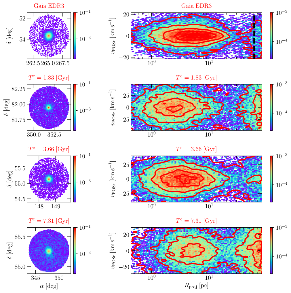
Now, we try to find any possible indication of tidal features, such as a stellar diffuse inner profile or tidal tails for NGC 6397 by comparing Gaia EDR3 with our simulated GCs. This comparison is done in two steps. First, in Figure 5, we investigate the inner profile in the sky plot of observed and simulated clusters. Second, in Figure 6, we analyze the outer regions of the clusters by considering the projected radial velocity as a function of the projected distance to the cluster centre. We describe these two steps in the following subsections.
5.2.1 Sky plot
In order to compare our simulation results with NGC 6397 using Gaia EDR3 data, we need to project our simulated GCs on the plane of sky, which was done using the Astropy Python package (Astropy Collaboration et al. 2013), assuming the observer is located at the Sun’s position. Figure 5 was then constructed by projecting our simulations in the plane of sky, and in this particular case, placing the GC at the same galactic position as observed today. This allows us to check if an effect of projection or an artifact of the close position of the cluster could blur the diffuse spatial distribution of our simulated GCs.
The first column in Figure 5 shows the observed GC, without interlopers, which was done after selecting the GC stars by filtering Gaia EDR3 with BALRoGO11 1 https://gitlab.com/eduardo-vitral/balrogo (Vitral 2021). We did not consider membership probabilities related to the projected distance (apart from allowing stars up to two degrees from the cluster centre) since one of our goals is to detect possible GC escapers, and therefore, our filters were based on proper motion and CMD regions only. We were also forced to keep stars with a low proper motion error (defined as in Lindegren et al. 2018) of half the velocity dispersion of the cluster, so the number of MW contaminants was reduced, which in turn led us to a cutting of roughly 20 mag.
Figure 5 clearly shows a very concentrated distribution of stars in NGC 6397 Gaia EDR3 data, in contrast with a strongly diffused profile of our GC in Run 3 at 10 Gyr. Although the tidal tails of the simulation seem too large to be perceived in a two degree sky plot, the inner shape of observed and simulated clusters are radically different. Our simulated GC exhibits an extended and distorted stellar distribution in its inner part due to the strong MW tidal field, whereas NGC 6397 seems to maintain a spherical compact shape.
5.2.2 Projected radial velocity
In Figure 6, we again compare Gaia EDR3 data (first row) with subsequent snapshots of our GC from Run 3, drowned in mock MW contaminants and projected in the plane of sky, but keeping the original distance to the Sun from each step of the simulation. The cut in Gaia EDR3 data was much less conservative this time, since we allowed all Gaia EDR3 stars within a 5- region around the bulk proper motion of the GC, which ensures that we do not miss possible GC stars which are part of tidal tails. This was done by accepting all stars satisfying:
| (3) |
where and are the mean proper motions of NGC 6397 in right ascension and declination, respectively, derived according to Vitral 2021, while and are the corresponding proper motions from the Gaia stars. In order to account for the uncertainties on the proper motions, we also added Gaia-like errors to our simulated cluster and interlopers according to the recipe from Vitral 2021. The selection of cluster members by considering fiducial regions on the proper motion space around the cluster bulk proper motion is a method largely employed in the literature, and have been extensively used in Gaia data (e.g., Gaia Collaboration et al. 2018; Vasiliev 2019; Baumgardt et al. 2019; Sollima 2020; Kundu et al. 2020 and more recently, Vasiliev & Baumgardt 2021 and Vitral 2021).
The fact that we employ no other data cleaning, nor exclude stars due to their positions on the sky or in the CMD surely allows for many interlopers. These contaminants can affect the distinction between GC stars and field stars, which can naturally blur imprints of tidal tails. In order to evaluate the impact of these contaminants, we created mock MW interlopers uniformly distributed in the sky according to Appendix A, and added them to our simulated data. We decided the position and the extent of the field stars proper motion distribution, which follows a Pearson VII symmetric distribution, by mimicking the field stars around NGC 6397.
Figure 6 clearly demonstrates that, during the formation of tidal tails for our simulated GC, a continuity in density for the projected radial proper motion along the projected radius emerges below the tidal radius of approximately 100 pc. It shows the presence of potential escapers due to MW tidal effects. In contrast, for NGC 6397, there is a clear cut-off at roughly 30 pc between GC stars and MW interlopers, and thus, no obvious tidal tails. Indeed, the density transition in the observed data seems to correspond to that of a cluster at the very beginning of its evolution in the MW tidal field, as the simulated cluster at 1.83 Gyr. Interestingly, the stellar streams detected recently by Ibata et al. 2020 seem to have a length comparable to our simulation at this stage of the cluster’s evolution (see Figure 4), even when taking into account projection effects as further explained in section 6.1.
According to Gaia EDR3 data, we state that there is no obvious sign of an ongoing intense tidal disruption for this cluster. We stress that we do manage, in spite of the MW contamination, to detect these tidal features of our simulated GC by looking at the projected radial velocity as a function of the projected distance.
5.3 Surface density profile
Finally, we compare the density profiles at the end of our simulations which survived for more than Gyr, with the density profile of NGC 6397, derived in Vitral & Mamon 2021, in Figure 7. We constructed these profiles by binning the simulated GCs with 50 log-spaced radial bins and considering a stellar mass of M⊙. One can see that for all the different simulations, the final profile (dashed) is much more diffuse than the observed profile, extending beyond the tidal radius of NGC 6397. Moreover, both Kolmogorov-Smirnov and Wilcoxon tests indicate strong confidence that the distributions are not the same, with respective values reaching an underflow (i.e. converging towards zero). We also fitted a Sérsic profile to our stripped simulated clusters depicted in Figure 7 and we found a Sérsic radius above 50 times greater than the value presented in Table 1. This indicates that the tidal disruption seen in our simulations is more advanced than any possible tidal disruption that NGC 6397 has suffered.
6 Discussion
Our observational data analysis establishes that several indicators such as the stellar distribution and the radial velocity along the projected radius of NGC 6397 seem to rule out the presence of extended tidal tails, contrary to the predictions of our simulations. Here, we provide and evaluate several solutions, which could explain the discrepancy between our simulations and the Gaia EDR3 observations of NGC 6397.
6.1 Projection effects

One of the possible explanations for the lack of tails in the observations could be a projection effect, since the tails could be aligned along the line-of-sight connecting the Sun and NGC 6397. If this is the case, the projection of these tails would be negligible on the sky plot of Figure 5, as well as in the outer projected radii of Figure 6.
In order to test this assumption, we refer to the work of Klimentowski et al. 2009 and Montuori et al. 2007, who analyzed the orientation of tidal tails in dwarf spheroidal galaxies and GCs, respectively, by studying the outcome of body simulations. Both studies report that in the vicinity of the dwarf or the GC, the tails are typically oriented towards the MW and not along the orbit (see Figures 2 and 3 from Montuori et al. 2007). Indeed, it is in the vicinity of those sources (i.e. at distances closer than 1 kpc) that the tails are denser and therefore most likely to be detectable. This is well suited for our analysis as we restrict our study to only two (five, in Figure 9) degrees around the cluster centre.
Therefore, we verify if the sky projection of the direction connecting the NGC 6397 and the MW centre is washed out due to an alignment problem (i.e. degrees in Figure 8). We derive degrees, which is sufficient for us to detect extended tidal tails, since the projection of such components would yield a length of roughly , with being the length of the tidal tails in the direction of the MW centre (see Figure 8). the large projection of the tails in the sky derived above is then an important argument for this bias to be neglected.
6.2 Limiting magnitude
Gaia EDR3, as well as its predecessor, has a magnitude limit of , which basically means that the faintest GC stars, with masses M⊙, are not taken into account. Naturally, fainter stars tend to occupy distances farther from the GC centre than brighter stars, due to mass segregation (Binney & Tremaine 2008), and such a relation has been robustly observed by Heyl et al. 2012 and Vitral & Mamon 2021 for NGC 6397. Therefore, one possibility is that NGC 6397 might have tidal tails which are just not detected by Gaia EDR3, as a consequence of how deep, in magnitude, its observations can probe. However, Vitral & Mamon 2021 found that, although the fainter stars do follow a more diffuse distribution in space, their radial extent is only about two times greater than the brighter stars (i.e. pc, see Table 1 for a comparison), which remains a small radial extent when compared to our simulated GC from Run 3 presenting a Sérsic radius of 200 pc and tidal tails of more than 1 kpc long in early stages of the cluster life.
6.2.1 Comparison with other globular clusters
We now test if this limiting magnitude could affect, for example, Figures 5 and 6, by blurring or erasing the contribution of faint stars in tidal tails drowned in MW contaminants. For that, we generate plots similar to Figure 6 for GCs known to have obvious tidal tails, such as Pal 5 (Odenkirchen et al. 2001) and NGC 5139 ( Cen, Ibata et al. 2019).
Indeed, our method was not able to detect strong imprints of the massive tidal tails of Pal 5, given that it is located at roughly 21.6 kpc away from the Sun. As Pal 5 is about nine times more distant than NGC 6397, the limiting magnitude of Gaia EDR3 prevents us from observing many of the faint stars that dominate the tails of the former cluster, whose apparent magnitude depends on their distance to us. Therefore, we decide to test our method with a closer GC, Cen, known to have important tidal tails (e.g. Ibata et al. 2019 and Sollima 2020), and whose distance and MW contamination are not too different from NGC 6397 (the values of distance to the Sun and galactocentric distance of Cen are 5.2 kpc and 6.4 kpc, respectively, Harris 2010). Since NGC 5139 is still more distant than NGC 6397, detecting any tidal imprints around it through our method from Figure 6 would indicate the reliability of this procedure.
The first row of Figure 9, which also selects all Gaia EDR3 stars within a 5- proper motion region, this time inside a five-degree cone search around Cen, shows that although the MW contamination does play a role in blurring the GC escapers, we are still able to observe the continuity in density, for the proper motion radial component along the projected radius, which indicates the presence of tidal arms. Even if Montuori et al. 2007 pointed out that Cen has tidal tails deviating from the galactocentric direction and extending toward the galactic plane, our method highlights the external structure. Besides, Cen in Figure 9 is similar to second and third snapshots of Figure 6. We display, in the second row, the similar plot of NGC 6397 for comparison. Thus, if ever NGC 6397 has extended tidal tails formed by fainter stars blurred by MW contamination, it would be curious if such an effect is not repeated for Cen.
For the observed NGC 6397 extending up to 5 degrees, which is the aperture usually probed in this kind of study (Sollima 2020), there is still a clear cut-off and no sign of tidal arms, but only of a stronger MW contamination at outer radii (see Figure 9). Indeed, Klimentowski et al. 2009 stress that the most evident signs of tidal structures will be seen closer to the analyzed source, where the stars are more clumped together.
6.3 Dark matter profile of the MW
In our MW mass model, we have assumed a NFW profile for the DM halo. However, an evidence for a DM core in the MW was claimed by Portail et al. 2017 in order to explain the high velocity dispersion of the stars in the Galactic bulge. They predicted a small DM core of few kpc in size. In all runs, the GC orbits around the MW centre at a distance between 5.1 and 9.2 kpc. As the GC does not orbit in the regions where a DM core can be produced by feedback (Lazar et al. 2020), it will not feel the dynamical impact of a different DM density profile for the MW. Moreover, we emphasize that the gravitational potential is dominated by stars of the bulge in this inner region of the MW. Therefore, varying the enclosed mass in the inner region of the MW is not a viable solution to efficiently delay the formation of tidal tails around the GC in order to reproduce the Gaia EDR3 observations.
6.4 GCs embedded in dark matter
We now discuss the possible influence of the presence of DM in GCs during their evolution. It has also been proposed that GCs may have a galactic origin, where GCs are formed within DM minihalos in the early Universe (e.g. Peebles 1984a; Bromm & Clarke 2002; Mashchenko & Sills 2005; Ricotti et al. 2016). Then, these GCs could have merged to later become a part of the present-day host galaxy.
Until now, these DM halos have not been detected. More precisely, it was pointed out that the ratio of the mass in DM to stars in several GCs is less than unity (Shin et al. 2013; Conroy et al. 2011; Ibata et al. 2013; Moore 1996; Baumgardt et al. 2009; Lane et al. 2010; Feng et al. 2012; Hurst et al. 2015). Even if GCs are proven not to have a significant amount of DM, it does not preclude them from having been formed originally within a DM minihalo. A natural explanation is that they have lost their DM over time. Indeed, there are several internal dynamical processes which could eject DM from GCs such as DM decay (Peter et al. 2010) and feedback processes (Pontzen & Governato 2012; Davis et al. 2014). It was also shown that GCs orbiting in the inner regions of their host galaxies may lose a large fraction of their primordial DM minihalo due to tidal stripping (e.g. Bromm & Clarke 2002; Mashchenko & Sills 2005; Saitoh et al. 2006; Bekki & Yong 2012). That is the reason why the main mechanism by which our GC could have lost its DM minihalo is through severe tidal interactions with our Galaxy given its current position. For instance, it was demonstrated that if the Fornax GCs were embedded in DM, they would have lost a large fraction of their DM minihalos, whose masses would have been in good agreement with the constraints for GCs (Boldrini et al. 2020). Nevertheless, GCs at a large distance from the MW centre could have retained a significant fraction of DM because it was not completely stripped by the Galaxy. Even if observations of these GCs such as NGC 2419 and MGC1 highlight that they do not possess significant DM today (Conroy et al. 2011; Ibata et al. 2013), it does not exclude the existence of DM in GCs but suggest that there is not necessarily a unique formation mechanism for GCs in general.
Contrary to our simulated GCs, which exhibit obvious stellar tidal tails, which are well extended in the sky, we argue that NGC 6397 does not possess such strong tidal imprints, based on Gaia EDR3 data (see Figures 6 and 9). It was claimed that these tidal structures should not form if they were embedded in DM minihalos (Grillmair et al. 1995; Moore 1996; Mashchenko & Sills 2005; Odenkirchen et al. 2003). Indeed, adding this dark component to this GC could help to avoid the formation of stellar tidal tails. Moreover, it was shown that DM minihalos following a core profile are much easier to disrupt tidally in galaxy than minihalos described by an NFW profile (Mashchenko & Sills 2005). A GC embedded in NFW DM minihalo could keep its stellar structure almost intact but be still dominated by DM in its outskirts (Heggie & Hut 1996; Baumgardt et al. 2009; Lane et al. 2010; Peñarrubia et al. 2017). It could be possible to detect the remnant of the DM halo by looking at the projected velocity dispersion profiles of stars (Peñarrubia et al. 2017). Indeed, the presence of DM will manifest itself in the form of a heating of the stars beyond the tidal radius. Figure 6 from Vitral & Mamon 2021 shows a clear increase in the dispersion profile of NGC 6397 beginning at roughly 17 arcmin (i.e. 20 per cent of the tidal radius).
We pointed out that Gaia EDR3 data reveals that stars in the central region of NGC 6397 seem to follow a spherical distribution (see Figure 5). Curiously, it was argued that a stellar cluster evolving inside a DM minihalo would have close to this sort of distribution in its denser part, where the stars dominate over DM (Mashchenko & Sills 2005). We stress that DM provides a potential solution to the case of NGC 6397. A DM minihalo could be responsible for both the inner spherical shape and the absence of tidal tails in this cluster, as the stellar part of a GC embedded in DM would be more resilient to tidal disruption.
6.5 Ex-situ origin
It was also suggested that nuclear star clusters of tidally-stripped galaxies may be the progenitors of GCs, especially massive ones such as G1 and Cen (Freeman 1993; Bekki & Freeman 2003; Bekki & Yong 2012; Böker 2008; Meylan et al. 2001). They are the most massive clusters of their parent galaxies, M31 and the MW, respectively. Nucleated dwarf galaxies can be transformed into GCs due to tidal stripping of the dwarfs by the strong gravitational field of galaxies (Bekki et al. 2002; Bekki & Freeman 2003). It is important to note that this scenario is also motivated by the presence of a far more complex stellar population in clusters such as Cen (three distinct populations, Pancino et al. 2003), compared to normal clusters. NGC 6397 hosts only two stellar populations (Milone et al. 2012).
Furthermore, these GC-like systems were embedded in DM halos (Taylor 2005; Böker et al. 2004; Walcher et al. 2005; Walcher et al. 2006). GCs originated from nucleated dwarfs have therefore formed outside the central regions of the MW. That is the reason why these GC-like systems can have no DM at the present day. In fact, most of the initial DM halo was stripped away from the GC during the first several orbits, even if they are massive at their birth (Wirth et al. 2020).
The fact that a GC may be a nuclear star cluster remnant could explain the absence of its stripping in the dense MW central region, but it is also used to argue that it may have an intermediate-mass black hole (IMBH) at its centre (Bahcall & Wolf 1976). Indeed, it was claimed that G1 and Cen could contain IMBHs with a mass of M⊙ (Gebhardt et al. 2002; Gebhardt et al. 2005; van der Marel & Anderson 2010). However, it was recently demonstrated that the presence of a central IMBH in NGC 6397 was ruled out, in favour of a diffuse dark inner sub-cluster of stellar remnants (Vitral & Mamon 2021), well explained by a strong concentration of faint white dwarfs (Kremer et al. 2021).
7 Conclusion
In this work, we performed -body simulations on GPU in an attempt to reproduce the past 10 Gyr of dynamical evolution of a globular cluster presenting similar characteristics to the nearby globular cluster NGC 6397, in the strong tidal field of a Milky Way-like galaxy. We considered a purely baryonic globular cluster, and we used the prescription from Baumgardt & Makino 2003 (Baumgardt & Makino 2003, see our equation (2), in order to access the corrected time of evolution of the cluster, while keeping a feasible mass resolution.
The intense background of dark matter and stars in our simulations is sufficient to disrupt the cluster in a Hubble time. We demonstrate that the lifetime of the simulated cluster depends mainly on its initial density profile and mass. More importantly, we find that more than 6 Gyr ago, right after the first third of the cluster’s life, all of our simulated GCs presented tidal tails, which extended farther than 1 kpc long. We subsequently compare our simulations and observations of NGC 6397 from Gaia EDR3 data. Despite its recent passage through the galactic disk (Rees & Cudworth 2003), we find that several indicators seem to rule out the presence of obvious tidal tails around NGC 6397. Since we believe that the analysis performed with Gaia EDR3 data was robust and contradictory to our simulations, where GCs exhibit extended tails, it is much more likely that the cause of such discrepancy is due to the origin scenario of the evolving cluster, as well as some of the environmental conditions of our simulations. Indeed, we have considered three main factors that could influence the formation of tidal tails in NGC 6397: the dark matter profile of the Milky Way, an extra-galactic origin for this globular cluster, as well as their formation in dark matter minihalos.
We argue that the most likely flaw of our simulation was to consider a purely baryonic globular cluster at the beginning of the simulation. In fact, when assuming a scenario where globular clusters are formed in a dark matter minihalo (Peebles & Dicke 1968; Peebles 1984a), we would expect it to protect the cluster stars against intense tidal stripping, which would act as a shield and be itself stripped instead of the luminous matter. The fact that we do not manage to robustly observe considerable amounts of dark matter in globular clusters, and particularly in NGC 6397, could be attributed to such initial dark matter minihalos being stripped by the combination of internal processes of the globular cluster such as stellar evolution and supernovae, and the intense tidal field of the Milky Way.
The future releases of the Gaia mission will undoubtedly shed light onto this mystery since more reliable and complete astrometry can help to robustly assign cluster membership probabilities to the stars in the field of the globular cluster, and thus, better trace escaping cluster stars. It will also allow us, by targeting the cluster outskirts, to probe the velocity dispersion in and beyond the tidal radius and thus test predictions concerning the formation of globular clusters in dark matter minihalos (e.g., Peñarrubia et al. 2017). In a future work, we intend to test this dark matter scenario in our simulations and therefore test if such initial conditions can adequately explain the absence of extended tidal tails in NGC 6397.
Acknowledgements
We thank the reviewer for their constructive feedback which helped to improve the quality of the manuscript. We thank Holger Baumgardt, Jorge Peñarrubia, Joseph Silk, David Valls-Gabaud and Gary Mamon for useful comments and suggestions to improve the quality of this work. We also thank Miki Yohei for providing us the non-public -body code, gothic. We would like also to thank Dante von Einzbern for his constructive suggestions on improving the manuscript.
Data availability
The data that support the plots within this paper and other findings of this study are available from the corresponding author upon reasonable request.
References
- Abadi et al. (2006) Abadi M. G., Navarro J. F., Steinmetz M., 2006, MNRAS, 365, 747
- Astropy Collaboration et al. (2013) Astropy Collaboration et al., 2013, A&A, 558, A33
- Bahcall & Wolf (1976) Bahcall J. N., Wolf R. A., 1976, ApJ, 209, 214
- Baumgardt & Makino (2003) Baumgardt H., Makino J., 2003, MNRAS, 340, 227
- Baumgardt et al. (2004) Baumgardt H., Makino J., Ebisuzaki T., 2004, ApJ, 613, 1133
- Baumgardt et al. (2009) Baumgardt H., Côté P., Hilker M., Rejkuba M., Mieske S., Djorgovski S. G., Stetson P., 2009, MNRAS, 396, 2051
- Baumgardt et al. (2019) Baumgardt H., Hilker M., Sollima A., Bellini A., 2019, MNRAS, 482, 5138
- Bekki & Freeman (2003) Bekki K., Freeman K. C., 2003, MNRAS, 346, L11
- Bekki & Yong (2012) Bekki K., Yong D., 2012, MNRAS, 419, 2063
- Bekki et al. (2002) Bekki K., Forbes D. A., Beasley M. A., Couch W. J., 2002, MNRAS, 335, 1176
- Bellini et al. (2014) Bellini A., et al., 2014, ApJ, 797, 115
- Bertin & Varri (2008) Bertin G., Varri A. L., 2008, ApJ, 689, 1005
- Binney & Tremaine (2008) Binney J., Tremaine S., 2008, Galactic Dynamics: Second Edition
- Böker (2008) Böker T., 2008, ApJ, 672, L111
- Böker et al. (2004) Böker T., Sarzi M., McLaughlin D. E., van der Marel R. P., Rix H.-W., Ho L. C., Shields J. C., 2004, AJ, 127, 105
- Boldrini et al. (2020) Boldrini P., Mohayaee R., Silk J., 2020, MNRAS, 492, 3169
- Bovy (2015) Bovy J., 2015, ApJS, 216, 29
- Bromm & Clarke (2002) Bromm V., Clarke C. J., 2002, ApJ, 566, L1
- Brown et al. (2018) Brown T. M., Casertano S., Strader J., Riess A., VandenBerg D. A., Soderblom D. R., Kalirai J., Salinas R., 2018, ApJ, 856, L6
- Bullock & Johnston (2005) Bullock J. S., Johnston K. V., 2005, ApJ, 635, 931
- Carretta et al. (2009) Carretta E., et al., 2009, A&A, 505, 117
- Ciotti & Bertin (1999) Ciotti L., Bertin G., 1999, A&A, 352, 447
- Conroy et al. (2011) Conroy C., Loeb A., Spergel D. N., 2011, ApJ, 741, 72
- Davis et al. (2014) Davis A. J., Khochfar S., Dalla Vecchia C., 2014, MNRAS, 443, 985
- Dehnen et al. (2004) Dehnen W., Odenkirchen M., Grebel E. K., Rix H.-W., 2004, AJ, 127, 2753
- Di Matteo et al. (2019) Di Matteo P., Haywood M., Lehnert M. D., Katz D., Khoperskov S., Snaith O. N., Gómez A., Robichon N., 2019, A&A, 632, A4
- Diemand et al. (2007) Diemand J., Kuhlen M., Madau P., 2007, ApJ, 657, 262
- Feng et al. (2012) Feng L., Yuan Q., Yin P.-F., Bi X.-J., Li M., 2012, J. Cosmology Astropart. Phys., 2012, 030
- Forbes & Bridges (2010) Forbes D. A., Bridges T., 2010, MNRAS, 404, 1203
- Freeman (1993) Freeman K. C., 1993, in Smith G. H., Brodie J. P., eds, Astronomical Society of the Pacific Conference Series Vol. 48, The Globular Cluster-Galaxy Connection. p. 608
- Gaia Collaboration et al. (2018) Gaia Collaboration et al., 2018, A&A, 616, A12
- Gaia Collaboration et al. (2020) Gaia Collaboration Brown A. G. A., Vallenari A., Prusti T., de Bruijne J. H. J., Babusiaux C., Biermann M., 2020, arXiv e-prints, p. arXiv:2012.01533
- Gebhardt et al. (2002) Gebhardt K., Rich R. M., Ho L. C., 2002, ApJ, 578, L41
- Gebhardt et al. (2005) Gebhardt K., Rich R. M., Ho L. C., 2005, ApJ, 634, 1093
- Gieles et al. (2021) Gieles M., Erkal D., Antonini F., Balbinot E., Peñarrubia J., 2021, arXiv e-prints, p. arXiv:2102.11348
- Gratton et al. (2019) Gratton R., Bragaglia A., Carretta E., D’Orazi V., Lucatello S., Sollima A., 2019, A&ARv, 27, 8
- Greene et al. (2019) Greene J. E., Strader J., Ho L. C., 2019, arXiv e-prints, p. arXiv:1911.09678
- Grillmair et al. (1995) Grillmair C. J., Freeman K. C., Irwin M., Quinn P. J., 1995, AJ, 109, 2553
- Harris (2010) Harris W. E., 2010, arXiv e-prints, p. arXiv:1012.3224
- Heggie & Giersz (2009) Heggie D. C., Giersz M., 2009, MNRAS, 397, L46
- Heggie & Hut (1996) Heggie D. C., Hut P., 1996, in Hut P., Makino J., eds, IAU Symposium Vol. 174, Dynamical Evolution of Star Clusters: Confrontation of Theory and Observations. p. 303 (arXiv:astro-ph/9511115)
- Hernquist (1990) Hernquist L., 1990, ApJ, 356, 359
- Heyl et al. (2012) Heyl J. S., et al., 2012, ApJ, 761, 51
- Hurst et al. (2015) Hurst T. J., Zentner A. R., Natarajan A., Badenes C., 2015, Phys. Rev. D, 91, 103514
- Husser et al. (2016) Husser T.-O., et al., 2016, A&A, 588, A148
- Ibata et al. (2013) Ibata R., Nipoti C., Sollima A., Bellazzini M., Chapman S. C., Dalessandro E., 2013, MNRAS, 428, 3648
- Ibata et al. (2019) Ibata R. A., Bellazzini M., Malhan K., Martin N., Bianchini P., 2019, Nature Astronomy, 3, 667
- Ibata et al. (2020) Ibata R., et al., 2020, arXiv e-prints, p. arXiv:2012.05245
- Irrgang et al. (2013) Irrgang A., Wilcox B., Tucker E., Schiefelbein L., 2013, A&A, 549, A137
- Kamann et al. (2016) Kamann S., et al., 2016, A&A, 588, A149
- King (1966) King I. R., 1966, AJ, 71, 64
- Klimentowski et al. (2009) Klimentowski J., Łokas E. L., Kazantzidis S., Mayer L., Mamon G. A., Prada F., 2009, MNRAS, 400, 2162
- Kremer et al. (2020) Kremer K., et al., 2020, ApJS, 247, 48
- Kremer et al. (2021) Kremer K., Rui N. Z., Weatherford N. C., Chatterjee S., Fragione G., Rasio F. A., Rodriguez C. L., Ye C. S., 2021, arXiv e-prints, p. arXiv:2104.11751
- Kundu et al. (2020) Kundu R., Navarrete C., Fernández-Trincado J. G., Minniti D., Singh H. P., Sbordone L., Piatti A. E., Reylé C., 2020, arXiv e-prints, p. arXiv:2011.10525
- Küpper et al. (2010) Küpper A. H. W., Kroupa P., Baumgardt H., Heggie D. C., 2010, MNRAS, 401, 105
- Küpper et al. (2012) Küpper A. H. W., Lane R. R., Heggie D. C., 2012, MNRAS, 420, 2700
- Lamers et al. (2010) Lamers H. J. G. L. M., Baumgardt H., Gieles M., 2010, MNRAS, 409, 305
- Lane et al. (2010) Lane R. R., et al., 2010, MNRAS, 406, 2732
- Lazar et al. (2020) Lazar A., et al., 2020, MNRAS, 497, 2393
- Leon et al. (2000) Leon S., Meylan G., Combes F., 2000, A&A, 359, 907
- Lima Neto et al. (1999) Lima Neto G. B., Gerbal D., Márquez I., 1999, MNRAS, 309, 481
- Lindegren et al. (2018) Lindegren L., et al., 2018, A&A, 616, A2
- Lovisi et al. (2012) Lovisi L., Mucciarelli A., Lanzoni B., Ferraro F. R., Gratton R., Dalessandro E., Contreras Ramos R., 2012, ApJ, 754, 91
- Lux et al. (2010) Lux H., Read J. I., Lake G., 2010, MNRAS, 406, 2312
- Marín-Franch et al. (2009) Marín-Franch A., et al., 2009, ApJ, 694, 1498
- Mashchenko & Sills (2005) Mashchenko S., Sills A., 2005, ApJ, 619, 258
- McMillan (2017) McMillan P. J., 2017, MNRAS, 465, 76
- Meylan et al. (2001) Meylan G., Sarajedini A., Jablonka P., Djorgovski S. G., Bridges T., Rich R. M., 2001, AJ, 122, 830
- Miki & Umemura (2017) Miki Y., Umemura M., 2017, New Astron., 52, 65
- Miki & Umemura (2018) Miki Y., Umemura M., 2018, MNRAS, 475, 2269
- Milone et al. (2012) Milone A. P., Marino A. F., Piotto G., Bedin L. R., Anderson J., Aparicio A., Cassisi S., Rich R. M., 2012, ApJ, 745, 27
- Montuori et al. (2007) Montuori M., Capuzzo-Dolcetta R., Di Matteo P., Lepinette A., Miocchi P., 2007, ApJ, 659, 1212
- Moore (1996) Moore B., 1996, ApJ, 461, L13
- Navarro et al. (1996) Navarro J. F., Frenk C. S., White S. D. M., 1996, ApJ, 462, 563
- Odenkirchen et al. (2001) Odenkirchen M., et al., 2001, ApJ, 548, L165
- Odenkirchen et al. (2003) Odenkirchen M., et al., 2003, AJ, 126, 2385
- Pancino et al. (2003) Pancino E., Seleznev A., Ferraro F. R., Bellazzini M., Piotto G., 2003, MNRAS, 345, 683
- Peñarrubia et al. (2009) Peñarrubia J., Walker M. G., Gilmore G., 2009, MNRAS, 399, 1275
- Peñarrubia et al. (2017) Peñarrubia J., Varri A. L., Breen P. G., Ferguson A. M. N., Sánchez-Janssen R., 2017, MNRAS, 471, L31
- Peebles (1984a) Peebles P. J. E., 1984a, in Audouze J., Tran Thanh Van J., eds, NATO Advanced Study Institute (ASI) Series C Vol. 117, Formation and Evolution of Galaxies and Large Structures in the Universe. p. 185
- Peebles (1984b) Peebles P. J. E., 1984b, ApJ, 277, 470
- Peebles & Dicke (1968) Peebles P. J. E., Dicke R. H., 1968, ApJ, 154, 891
- Peter et al. (2010) Peter A. H. G., Moody C. E., Kamionkowski M., 2010, Phys. Rev. D, 81, 103501
- Pontzen & Governato (2012) Pontzen A., Governato F., 2012, MNRAS, 421, 3464
- Portail et al. (2017) Portail M., Gerhard O., Wegg C., Ness M., 2017, MNRAS, 465, 1621
- Prugniel & Simien (1997) Prugniel P., Simien F., 1997, A&A, 321, 111
- Rees & Cudworth (2003) Rees R. F., Cudworth K. M., 2003, in American Astronomical Society Meeting Abstracts. p. 10.06
- Ricotti et al. (2016) Ricotti M., Parry O. H., Gnedin N. Y., 2016, ApJ, 831, 204
- Saitoh et al. (2006) Saitoh T. R., Koda J., Okamoto T., Wada K., Habe A., 2006, ApJ, 640, 22
- Searle & Zinn (1978) Searle L., Zinn R., 1978, ApJ, 225, 357
- Sérsic (1963) Sérsic J. L., 1963, Bull. Assoc. Argentina de Astron., 6, 41
- Shin et al. (2013) Shin J., Kim S. S., Lee Y.-W., 2013, Journal of Korean Astronomical Society, 46, 173
- Sollima (2020) Sollima A., 2020, MNRAS, 495, 2222
- Springel (2005) Springel V., 2005, MNRAS, 364, 1105
- Taylor (2005) Taylor M. B., 2005, TOPCAT & STIL: Starlink Table/VOTable Processing Software. p. 29
- Vasiliev (2019) Vasiliev E., 2019, MNRAS, 484, 2832
- Vasiliev & Baumgardt (2021) Vasiliev E., Baumgardt H., 2021, arXiv e-prints, p. arXiv:2102.09568
- Vitral (2021) Vitral E., 2021, MNRAS, 504, 1355
- Vitral & Mamon (2021) Vitral E., Mamon G. A., 2021, A&A, 646, A63
- Walcher et al. (2005) Walcher C. J., et al., 2005, ApJ, 618, 237
- Walcher et al. (2006) Walcher C. J., Böker T., Charlot S., Ho L. C., Rix H. W., Rossa J., Shields J. C., van der Marel R. P., 2006, ApJ, 649, 692
- Wan et al. (2021) Wan Z., et al., 2021, MNRAS, 502, 4513
- Watkins et al. (2015a) Watkins L. L., van der Marel R. P., Bellini A., Anderson J., 2015a, ApJ, 803, 29
- Watkins et al. (2015b) Watkins L. L., van der Marel R. P., Bellini A., Anderson J., 2015b, ApJ, 812, 149
- Widrow et al. (2008) Widrow L. M., Pym B., Dubinski J., 2008, ApJ, 679, 1239
- Wirth et al. (2020) Wirth H., Bekki K., Hayashi K., 2020, MNRAS, 496, L70
- van der Marel & Anderson (2010) van der Marel R. P., Anderson J., 2010, ApJ, 710, 1063
Appendix A Mock Milky Way interlopers
In this appendix, we describe how we generated Milky Way interlopers for our simulated globular clusters in Figure 6. The general method is described in section 2.6 of Vitral 2021. In addition, we describe here how we decided the input parameters of this method such as the interlopers maximum projected radius, bulk proper motions and their number.
A.1 Spatial distribution and proper motions
We created stars uniformly distributed in a spherical cap of projected radius , where is the maximum projected radius of our Gaia EDR3 data in Figure 6 (i.e., 2 degrees), and and are the distances of the simulated and observed clusters, respectively, with respect to an observer located at the Sun.
The number of interlopers was naively selected by taking an approximate interloper fraction in the region limited by , calculated by considering the number of GC stars as the stellar count in the Gaia cone search minus , with (the interlopers surface density) assumed constant and estimated as the surface density of the whole data beyond twelve arcmin (about three times the Sérsic radius). This interloper fraction was used with respect to the number of stars in the simulation having projected radius smaller than . At the end, we selected randomly, among all stars in the subset, the same number of stars present in the plot of NGC 6397, so we could mimic the incompleteness of the data.
The proper motions of the field stars created above follows a Pearson VII symmetric distribution with parameters similar to the ones of NGC 6397 Milky Way interlopers. Notably, the distance of the interloper bulk proper motion was taken as , with the one dimensional velocity dispersion in proper motions. The velocity dispersion and Pearson VII slope (see Vitral 2021 for details) were chosen to be similar to the values from the interlopers around NGC 6397 (i.e., and ).