ASFlow: Unsupervised Optical Flow Learning with Adaptive Pyramid Sampling
Abstract
We present an unsupervised optical flow estimation method by proposing an adaptive pyramid sampling in the deep pyramid network. Specifically, in the pyramid downsampling, we propose an Content Aware Pooling (CAP) module, which promotes local feature gathering by avoiding cross region pooling, so that the learned features become more representative. In the pyramid upsampling, we propose an Adaptive Flow Upsampling (AFU) module, where cross edge interpolation can be avoided, producing sharp motion boundaries. Equipped with these two modules, our method achieves the best performance for unsupervised optical flow estimation on multiple leading benchmarks, including MPI-SIntel, KITTI 2012 and KITTI 2015. Particuarlly, we achieve EPE=1.5 on KITTI 2012 and F1=9.67% KITTI 2015, which outperform the previous state-of-the-art methods by 16.7% and 13.1%, respectively.
1 Introduction
Optical flow estimation is a long lasting research topic since proposed by Horn and Schunck [6]. It is a fundamental technique for many computer vision applications [13, 1, 29]. Early methods optimize the pre-defined energy functions with various assumptions and constraints [32, 33, 31, 28]. The learning-based optical flow methods become more popular than the traditional variational-based counterparts due to their leading performances in benchmark evaluations and real-time inference speed.
The DNN-based methods can be classified into supervised [3, 25, 8, 34, 9] and unsupervised [22, 19, 42, 18, 14] approaches. The training of supervised methods require the ground-truth flow labels, which is hard to obtain. As a result, these models are primarily trained on large-scale synthetic datasets [3, 2], because obtaining ground-truth annotations for real-world scenarios is prohibitively expensive. Consequently, the supervised methods may suffer from domain transfer problems, where the synthesized images are different from the real ones.
In unsupervised methods, the ground-truth annotations are not necessary. The photometric loss is optimized by warping one image to the other with predicted optical flows. Without the label guidance, occlusions and motion boundaries need special attentions during the unsupervised training process [14, 21].


The pyramid structure is popular in the optical flow learning, where global and local motions can be estimated in a coarse-to-fine manner. We notice that there are two components that should be improved in the pyramid structure [34, 9]. One is related to the pyramid downsampling and the other is the upsampling.
In the process of pyramid downsampling, the network adopts striding in convolution (SIC) or the pooling to decrease the feature sizes. However, the striding or pooling is fixed with a rectangular size, which may not be optimal for the feature information gathering. Considering that, a rectangle may span different image regions, where multiple irrelevant values are forced to gather together, picking one of them may not be optimal, yielding values that are less representative. On the other side, in the pyramid upsampling, the flows are interpolated from coarse-to-fine. However, such an interpolation may cross image edges, resulting in the blur effects in the estimated flows. Even worse, such errors will be propagated and aggregated when the scale becomes finer.
Based on the above observations, we propose an Adaptive Pyramid Sampling approach to upgrade the pyramid network structure, including a Content Aware Pooling (CAP) module for the pyramid downsampling and an Adaptive Flow Upsampling (AFU) module for the pyramid upsampling. The CAP can automatically group image features, such that the similar features can be gathered locally before the downsampling. With our CAP, the learned features become more representative, so as to promote the overall performance. On the other side, the AFU module interpolates the flows adaptively, where cross edge interpolation can be avoided, leading to sharper flows at motion boundaries. Specifically, in the AFU, we propose a sampling regularization loss to constrain the learned adaptive sampling maps, where the upsampled flow fields can better fit the object boundaries.
Fig. 1 provides some visualization results on Sintel Clean dataset. Specifically, Fig. 1(a) shows some feature similarity maps. We extract features from source and target images. We choose one feature vector at a position (marked in red cross) from the source image and calculate its similarity with all features at the target image. We plot the similarity as a heat map, where high similarity values are depicted in red. As seen, with our CAP, the feature at the ‘red cross’ is quite different from the features at the other places. In contrast, without our CAP, features at many different places also have high similarity values. Therefore, our model can learn more representative features with the proposed content aware pooling. Fig. 1(b) shows our predicted optical flow compared with other unsupervised methods. As can be seen, with the help of AFU, the interpolation can produce sharp motion boundaries. Equipped with CAP and AFU, the classical pyramid network has been upgraded, producing leading performance both quantitatively and qualitatively when evaluated on the flow benchmarks [2, 4, 23]. To sum up, our main contributions include:
- •
We propose a Content Aware Pooling (CAP) module for the pyramid downampling. The CAP can assemble similar features locally, improving the capability of feature representation substantially.
- •
We propose an Adaptive Flow Upsampling (AFU) module for the pyramid upsampling, where the blurs caused by cross-edge interpolation can be avoided, yielding sharper motion boundaries.
- •
We achieve superior performance over the state-of-the-art unsupervised methods, evaluated on multiple leading benchmarks.
2 Related Work
2.1 Supervised Deep Optical Flow
Supervised methods require the annotated ground-truth flow labels to train the network [7, 41]. FlowNet [3, 10] was first proposed by training on the flying chair dataset [3]. PWC-Net adopted the pyramid network that learns the motion from carose to fine, which calculates cost volumes at each pyramid level [34]. LiteFlowNet proposed to build lightweight networks for the efficiency [8]. IRR-PWC propsoed an iterative residual refinement scheme in the pyramid network [9]. Recently, RAFT [35] proposed to recurrently estimate flow fields on 4D correlation volumes, achieving state-of-the-art performance.
2.2 Unsupervised Deep Optical Flow
Unsupervised methods directly minimize the difference between two input images, by warping one to the other with predicted flow vectors. In this way, there is no need of ground-truth labels. However, the training becomes more difficult than supervised methods. Different methods with different focus have been proposed, including occlusion-aware losses by forward-backward check [22] and range-map occlusion check [38], census transform constrain [27], multi-frame formulation [12], data argumentation [18], data distillation [19, 20], epipolar constrain [42], depth constrains [26, 43] and feature similarity constrain [11]. By integrating multiple components, UFlow achieves the leading performance on multiple benchmarks [14].
2.3 Image Guided Upsampling
Our method is also related to the edge-aware interpolation and upsampling, such as joint bilateral upsampling [15] and guided image filtering [5]. Apart from the traditional methods, CNN approaches have also been attempted to extract guidance feature or guidance filter for upsampling [17, 39, 30]. We compare our AFU module with these opponents to demonstrate its effectiveness.

3 Algorithm
In this section, we first provide an overview of the network architecture of our method in Sec. 3.1. Then we introduce the proposed Content Aware Pooling (CAP) module in Sec. 3.2 and Adaptive Flow Upsampling (AFU) module in Sec. 3.3. Finally, we describe the loss functions used for unsupervised training in Sec. 3.4.
3.1 Network Architecture
The pipeline of the proposed network is illustrated in Fig. 2. It takes two frames and as inputs and produces an optical flow field that describes the motion of each pixel in towards . The whole network contains three parts: an adaptive sub-net, a siamese feature encoder and a flow decoder.
First, we use the adaptive sub-net to extract multi-scale adaptive sampling maps which will be used later in the CAP module and the AFU module:
| (1) |
where is our adaptive sub-net, is the index of each scale and small number represents the coarse scale, , and are adaptive sampling maps. In our implementation, the adaptive sub-net is designed as a simple U-Net structure detailed in our supplementary files.
Second, in the siamese feature encoder, we extract multi-scale feature pairs from the input images to cover both global and local information, which is formulated as:
| (2) | ||||
| (3) |
where is index of the input images, represents the proposed CAP module, is the downsampled feature of , and is a convolution layer.
After the feature encoding process, we estimate flow fields by the flow decoder formulated as follows:
| (4) | ||||
| (5) |
where represents our AFU module, is the upsampled flow from scale and is a flow estimator. Specifically, the flow estimator is designed following the recent work UFlow [14], which contains feature warping, correlation layer, cost volume normalization, a dense convolution block and a dilated convolution block.
Generally, convolution layers with stride are used to downscale feature maps. However, the regular downsampling method based on sliding windows may fuse features from different objects, reducing the matching accuracy of pair-wise correlation estimation. To tackle this issue, we propose CAP module to automatically group similar features in downsampling process, referred to as content aware pooling. Besides, we notice that the commonly used bilinear upsampling may introduce interpolation errors and blur artifacts during decoding process. Thus, the AFU module is proposed to ease this problem by adaptively interpolating flow fields with learnable weights. The details of these two modules are presented in Sec. 3.2 and Sec. 3.3.

3.2 Content Aware Pooling
As mentioned above, CAP module is proposed to automatically group similar features in the pooling process. The illustration of our CAP is shown in Fig. 4. The input is a high resolution feature map with size of , and an adaptive sampling map with size of , in which channels are used as sampling scores and the rest 2 channels are used as the control parameter and in our adaptive gumbel softmax. The output is a downsampled feature map with size of , where denotes the channel number and is the sampling rate, typically set to 2 in feature encoding process.
For each feature vector at spatial position , we calculate a sampling probability kernel from , which indicates the probability of contributing to the neighbouring region of its corresponding position in the low resolution feature . Then we generate the feature by grouping and accumulating all feature vectors in according to their sampling probability (the ‘’ and ‘Add’ operation in Fig. 4):
| (6) |
where is a set of pixels in whose sampling probability kernel covers position in .
In order to avoid feature grouping across different regions, we use adaptive gumbel softmax [24, 37] to suppress small probabilities when producing sampling probability kernels. The adaptive sampling map is first splitted as sampling scores and control parameters and to control the distribution tendency of sampling kernels, where is channel index and is spatial coordinate. In summary, the adaptive gumbel softmax can be formulated as follows:
| (7) | ||||
| (8) |
where is a constant to avoid zero denominator and is the transformed sampling score.
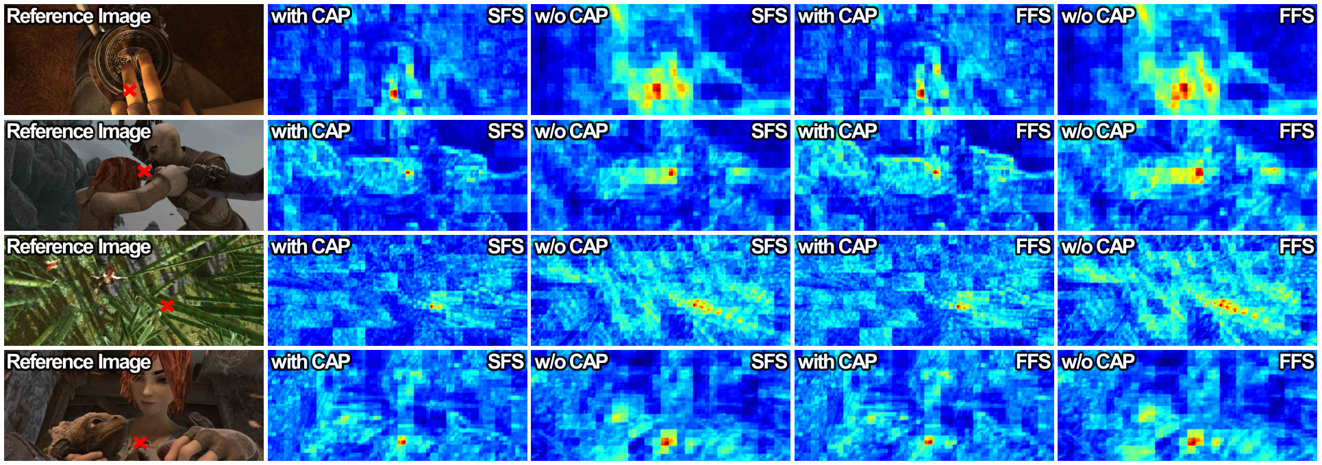
Fig. 3 provides some visualizations of content aware pooling results by comparing our CAP module with conventional striding in convolution (SIC). We first interpolate pyramid features into the image size and concatenate them together. Then feature vector in located by the red cross is selected to calculate cosine similarity with features of and , which is the self feature similarity (SFS) map and the forward feature similarity (FFS) map, respectively. The SFS map reveals the discriminative ability of the encoded features and the FFS map reveals the matching ability between feature pairs. From Fig. 3, we can see that feature extracted by SIC method is likely to be similar with neighbor objects, while feature by our CAP module is only similar with its corresponding feature vector.
| Method | KITTI 2012 | KITTI 2015 | Sintel Clean | Sintel Final | |||||
|---|---|---|---|---|---|---|---|---|---|
| train | test | train | test (F1-all) | train | test | train | test | ||
| Supervised | FlowNetS [3] | 8.26 | – | – | – | 4.50 | 7.42 | 5.45 | 8.43 |
| FlowNetS+ft [3] | 7.52 | 9.1 | – | – | (3.66) | 6.96 | (4.44) | 7.76 | |
| SpyNet [25] | 9.12 | – | – | – | 4.12 | 6.69 | 5.57 | 8.43 | |
| SpyNet+ft [25] | 8.25 | 10.1 | – | 35.07% | (3.17) | 6.64 | (4.32) | 8.36 | |
| LiteFlowNet [8] | 4.25 | – | 10.46 | – | 2.52 | – | 4.05 | – | |
| LiteFlowNet+ft [8] | (1.26) | 1.7 | (2.16) | 10.24% | (1.64) | 4.86 | (2.23) | 6.09 | |
| PWC-Net [34] | 4.57 | – | 13.20 | – | 3.33 | – | 4.59 | – | |
| PWC-Net+ft [34] | (1.45) | 1.7 | (2.16) | 9.60% | (1.70) | 3.86 | (2.21) | 5.13 | |
| IRR-PWC+ft [9] | – | – | (1.63) | 7.65% | (1.92) | 3.84 | (2.51) | 4.58 | |
| RAFT [35] | – | – | 5.54 | – | 1.63 | – | 2.83 | – | |
| RAFT-ft [35] | – | – | – | 6.30% | – | 2.42 | – | 3.39 | |
| Unsupervised | BackToBasic [40] | 11.30 | 9.9 | – | – | – | – | – | – |
| DSTFlow [27] | 10.43 | 12.4 | 16.79 | 39% | (6.16) | 10.41 | (6.81) | 11.27 | |
| UnFlow [22] | 3.29 | – | 8.10 | 23.3% | – | 9.38 | (7.91) | 10.22 | |
| OAFlow [38] | 3.55 | 4.2 | 8.88 | 31.2% | (4.03) | 7.95 | (5.95) | 9.15 | |
| Back2Future [12] | – | – | 6.59 | 22.94% | (3.89) | 7.23 | (5.52) | 8.81 | |
| NLFlow [36] | 3.02 | 4.5 | 6.05 | 22.75% | (2.58) | 7.12 | (3.85) | 8.51 | |
| DDFlow [19] | 2.35 | 3.0 | 5.72 | 14.29% | (2.92) | 6.18 | (3.98) | 7.40 | |
| EpiFlow [42] | (2.51) | 3.4 | (5.55) | 16.95% | (3.54) | 7.00 | (4.99) | 8.51 | |
| SelFlow [20] | 1.69 | 2.2 | 4.84 | 14.19% | (2.88) | 6.56 | (3.87) | 6.57 | |
| STFlow [36] | 1.64 | 1.9 | 3.56 | 13.83% | (2.91) | 6.12 | (3.59) | 6.63 | |
| ARFlow [18] | 1.44 | 1.8 | 2.85 | 11.80% | (2.79) | 4.78 | (3.87) | 5.89 | |
| SimFlow [11] | – | – | 5.19 | 13.38% | (2.86) | 5.92 | (3.57) | 6.92 | |
| UFlow [14] | 1.68 | 1.9 | 2.71 | 11.13% | (2.50) | 5.21 | (3.39) | 6.50 | |
| ASFlow(ours) | 1.26 | 1.5 | 2.47 | 9.67% | (2.40) | 4.56 | (2.89) | 5.86 | |
3.3 Adaptive Flow Upsampling
The conventional bilinear upsampling method may interpolate flow vectors across object boundaries leading to blur artifacts and errors during flow decoding process. To solve this problem, we design an adaptive flow upsampling module to adaptively interpolate flow fields with learnable weights. The detail of our AFU module is shown in Fig. 5. Given a low resolution flow field of size and a high resolution adaptive sampling map with size of , our goal is to produce a high resolution flow field with size of . We define as a spatial coordinate in and as its corresponding neighbors in . The flow vectors in high resolution flow field can be calculated by the following formulation (the ‘’ and ‘Assign’ operation in Fig. 5):
| (9) |
where is a sampling probability kernel generated from to indicate the contribution probability of to . The flow vectors in high resolution flow field is generated by adaptively fusing flow vectors in low resolution flow field based on sampling probability kernels. Note that, in order to suppress the probability of flow fusion across edges, we use adaptive gumbel softmax as in Eq. 7 and Eq. 8 to produce the kernels, where small probabilities are compressed to zeros.
3.4 Unsupervised Losses
In order to train our network in unsupervised setting where ground-truth is not available, we use a set of unsupervised losses as our training objective. Our main objective is the photometric loss , which is designed based on the brightness constancy assumption that the object appearance should be invariable in input frames. However, occlusion regions caused by moving objects can not be optimized by the photometric loss. We explicitly exclude these regions in the photometric loss by forward-backward consistency checking [22]. As a result, the photometric loss is formulated as follows:
| (10) |
where is the occlusion mask generated by forward-backward consistency checking. ‘’ indicates the non-occluded pixel and ‘’ means the occluded pixel. is the robust penalty function [19]: in which and are set to 0.4 and 0.01.
Following previous works, several loss functions are used to train our model, including the edge-aware smooth loss that improves the smoothness of output flow field [38], the census loss that increases the robustness under illumination changes [22], the boundary dilated warping loss to learn motions towards outside the image plane [21], the augmentation regularization loss that introduces the equivariance constrain to encourage the robustness to variations [18].
In order to ensure the upsampled flow fields to better fit object boundaries, we design a sampling regularization loss to constrain the learned adaptive sampling maps . We first downscale the input image to , whose size is the same as . Then we iteratively upsample the downscaled image and compute a reconstruction loss with the original image, which is formulated as follows:
| (11) | ||||
| (12) |
where is the reconstructed image by the iterative upsampling process described in Eq. 11.
Eventually, our loss function is a weighted combination of above individual loss terms:
| (13) |
where , , and are hyper-parameters, set to , , , in our experiments.

| CL | BDWL | ARL | CAP | AFU | KITTI 2012 | KITTI 2015 | Sintel Clean | Sintel Final | ||||||||
|---|---|---|---|---|---|---|---|---|---|---|---|---|---|---|---|---|
| ALL | NOC | OCC | ALL | NOC | OCC | ALL | NOC | OCC | ALL | NOC | OCC | |||||
| 4.52 | 1.76 | 19.63 | 7.58 | 2.46 | 30.43 | (3.52) | (1.87) | (12.9) | (4.19) | (2.59) | (13.64) | |||||
| ✓ | 3.39 | 1.09 | 16.58 | 6.89 | 2.20 | 28.12 | (3.41) | (1.62) | (13.5) | (3.85) | (2.17) | (13.71) | ||||
| ✓ | ✓ | 1.42 | 0.91 | 4.39 | 3.00 | 2.12 | 6.89 | (2.84) | (1.50) | (10.6) | (3.60) | (2.28) | (11.52) | |||
| ✓ | ✓ | ✓ | 1.37 | 0.93 | 3.98 | 2.64 | 1.96 | 6.01 | (2.61) | (1.33) | (10.1) | (3.17) | (1.92) | (10.70) | ||
| ✓ | ✓ | ✓ | ✓ | 1.29 | 0.89 | 3.78 | 2.53 | 1.98 | 5.16 | (2.51) | (1.27) | (9.79) | (2.98) | (1.79) | (9.98) | |
| ✓ | ✓ | ✓ | ✓ | 1.30 | 0.88 | 3.82 | 2.57 | 1.99 | 5.08 | (2.46) | (1.23) | (9.63) | (2.94) | (1.73) | (10.07) | |
| ✓ | ✓ | ✓ | ✓ | ✓ | 1.26 | 0.87 | 3.72 | 2.47 | 1.93 | 5.02 | (2.40) | (1.20) | (9.36) | (2.89) | (1.71) | (9.89) |
4 Experimental Results
4.1 Datasets and Implementation Details
We conduct comprehensive experiments on four widely-uesd optical flow benchmarks, including MPI-Sintel [2], KITTI 2012 [4], and KITTI 2015 [23]. MPI-Sintel contains 1,041 training image pairs extracted from the rendered open-source movie, divided into ‘Clean’ and ‘Final’ passes. Following previous works [14, 11, 18], we use both versions of rendering images to train our model. For KITTI 2012 and 2015, we first use the 28,058 image pairs from KITTI raw dataset to pre-train the model, and then perform finetuning on multi-view extension data.
The implementation of the proposed ASFlow is based on PyTorch toolbox. We train our model on 2 NVIDIA GeForce GTX 2080Ti GPUs for about 1000k iterations. For better generalization, we follow previous work [18] to use basic data augmentation strategies like random crop and horizontal flip for training. The standard evaluation metrics, i.e., average endpoint error (EPE) and the percentage of erroneous pixels (F1-measure), are used to evaluate the performance of the predicted optical flow.
4.2 Comparison with State-of-the-Arts
In Tab. 1, We compare our method with State-of-the-Art (SOTA) works, including both of supervised and unsupervised methods, on four widely-used datasets. The best unsupervised method is marked in bold and the second best is marked in blue for better comparison.
Comparison with Unsupervised Methods.
As shown in Tab. 1, our ASFlow consistently achieves better performance than other methods on four standard benchmarks. Specifically, our method achieves an EPE error of 1.5 on KITTI 2012 test set, which surpasses previous top-ranked methods UFlow [14] and ARFLow [18] by around 21.1% (1.9 1.5) and 16.7% (1.8 1.5), respectively. For KITTI 2015 online evaluation, our method set new records of 2.47 in EPE on training set and 9.67% in F1-measure, which outperforms previous methods by a large margin. On the most challenging dataset MPI-Sintel, our method achieves EPE scores of 4.56 on ‘Clean’ pass for online testing. It obtains EPE = 5.86 on ‘Final’ pass, outperformimg previous top methods SimFlow [11] and UFlow [14] by 1.06 and 0.64 in terms of EPE. It is worth noting that our method is the first one to achieve the best results on all benchmarks, as shown in each line of Tab. 1 (best viewed in colors).
Comparison with Supervised Methods.
We also report the results of representative supervised methods for comprehensive comparison, see Tab. 1. For cross domain evaluation, we consider the ground-truth of optical flow is not available for training. Thus, the supervised models are trained on synthetic data such as Flying Chairs [3] and Flying Chairs occ [9], while the training procedure of the unsupervised methods can be directly performed only using target domain images. As can be seen, our method achieves better performance than all the supervised methods. Especially in real scenarios like KITTI 2015 dataset, it significantly outperforms the well-known supervised methods like LiteFlowNet [8], PWC-Net [34] and RAFT [35] by a large margin (7.99, 10.73 and 3.07 in EPE, respectively).
As for in-domain evaluation, our method generally achieve competitive performance with the supervised methods. Specially, on KITTI 2012 and 2015 datasets, our method achieves 1.5 in EPE and 9.67% in F1-measure, which surprisingly exceed the recent supervised method like and LiteFlowNet [8].
4.3 Ablation Study
In this section, we conduct a series of ablation expriments to evaluate each component in the proposed network. Following [20, 11], we train our model on train sets of KITTI and MPI-Sintel. The EPE error over all pixels (ALL), non-occluded pixels (NOC) and occluded pixels (OCC) are reported for quantitative comparisons.
Unsupervised Components.
Following the success of prior works [21, 22, 21], we employ some effective components to boost the training of our model in an unsupervised manner. As shown in the first line of Tab. 2, we first train a baseline model using photometric loss and smooth loss, without the proposed modules. After adding census loss [22] (CL), boundary dilated warping loss [21] (BDWL) and augmentation regularization loss (ARL), it obtains consistent improvements by three metrics on all datasets, which demonstrates these three modules benefit to boosting a better prediction. Meanwhile, the performance of this model (CL + BDWL + ARL) is equivalent to that reported in previous best method UFlow [14]. In addition, replacing the original striding strategy by our CAP in the each stage of encoder network greatly improves the performance. Similarly, we append our AFU module on decoders, and observe that the three metrics are clearly reduced (the lower the better). Finally, we fully equip the model with both of CAP and AFU, which brings about 10% performance improvement.
| Method | KITTI 2012 | KITTI 2015 | Sintel Clean | Sintel Final |
|---|---|---|---|---|
| Bilinear | 1.29 | 2.53 | (2.51) | (2.98) |
| JBU [15] | 1.51 | 3.00 | (2.66) | (2.98) |
| GF [5] | 1.40 | 2.90 | (2.72) | (2.92) |
| DJF [16] | 1.36 | 2.79 | (2.75) | (3.20) |
| DGF [39] | 1.41 | 3.14 | (2.69) | (3.05) |
| PAC [30] | 1.42 | 2.65 | (2.58) | (2.95) |
| AFU | 1.28 | 2.52 | (2.45) | (2.90) |
| AFU-RL | 1.26 | 2.47 | (2.40) | (2.89) |
| Method | KITTI 2012 | KITTI 2015 | Sintel Clean | Sintel Final |
|---|---|---|---|---|
| Bilinear | 1.51 | 2.81 | (2.75) | (3.20) |
| AVE | 1.39 | 2.75 | (2.66) | (2.98) |
| MAX | 1.40 | 2.69 | (2.72) | (3.02) |
| SIC | 1.30 | 2.57 | (2.46) | (2.94) |
| CAP | 1.26 | 2.47 | (2.40) | (2.89) |
Ablation for Upsampling Modules.
There have been several works attempt to propose general upsampling operations based on image information, such as JBU [15], GF [5], DJF [16], DGF [39] and PAC [30]. However, these methods are not suitable to this challenging task. Here we propose a task specific upsampling strategy to better serve the need of optical flow upsampling. To verify the effect of our method, we carry out extensive comparisons with the upasampling methods. Specifically, we build a simple pyramid network with the same loss function, and repetitively change upsampling operations with the modules mentioned above for fair comparison. As we can see in Tab. 3, our AFU achieves the best performance over all the competitors. This is because AFU can adaptively interpolate flow fields with learnable weights in pyramid decoders, so that the blur artifacts caused by cross-edge interpolation can be avoided, see column 4 of Fig. 7.
Ablation for Feature Pooling Strategies.
Tab. 4 reports the comparison of our CAP with typical pooling strategies, including average pooling (AVE), max pooling (MAX), and striding in convolution (SIC). For fair comparison, all the experiments are conducted under the same setting. As we can see, our CAP consistently obtain better scores than others on four datasets. As mentioned in Sec. 3.2, the features are adaptively grouped based on content and appearance similarity, which helps the network to maintain spatial details of different objects. Experimental results demonstrate the obtained distinctive information is crucial for recovering the optical flow on thin stuffs as shown in Fig. 7 (first sample, column 3 and 5).
5 Conclusion
We have presented ASFlow, an adaptive pyramid sampling method for unsupervised optical flow estimation. Two modules have been proposed, content aware pooling (CAP) for the pyramid downsampling and adaptive flow upsampling (AFU) for the upsampling. We compare our method with previous representative optical flow methods on the several leading benchmarks. In the further, we will explore the proposed two modules in the other applications, especially the CAP for the high-level vision tasks.
References
- [1] Aseem Behl, Omid Hosseini Jafari, Siva Karthik Mustikovela, Hassan Abu Alhaija, Carsten Rother, and Andreas Geiger. Bounding boxes, segmentations and object coordinates: How important is recognition for 3d scene flow estimation in autonomous driving scenarios? In Proc. ICCV, pages 2593–2602, 2017.
- [2] Daniel Butler, Jonas Wulff, Garrett Stanley, and Michael Black. A naturalistic open source movie for optical flow evaluation. In Proc. ECCV, pages 611–625, 2012.
- [3] Alexey Dosovitskiy, Philipp Fischer, Eddy Ilg, Philip Hausser, Caner Hazirbas, Vladimir Golkov, Patrick van der Smagt, Daniel Cremers, and Thomas Brox. Flownet: Learning optical flow with convolutional networks. In Proc. ICCV, pages 2758–2766, 2015.
- [4] A. Geiger, P. Lenz, and R. Urtasun. Are we ready for autonomous driving? the kitti vision benchmark suite. In Proc. CVPR, pages 3354–3361, 2012.
- [5] Kaiming He, Jian Sun, and Xiaoou Tang. Guided image filtering. In European conference on computer vision, pages 1–14. Springer, 2010.
- [6] Berthold KP Horn and Brian G Schunck. Determining optical flow. Artificial intelligence, 17(1-3):185–203, 1981.
- [7] Tak-Wai Hui and Chen Change Loy. Liteflownet3: Resolving correspondence ambiguity for more accurate optical flow estimation. In Proc. ECCV, pages 169–184, 2020.
- [8] Tak-Wai Hui, Xiaoou Tang, and Chen Change Loy. Liteflownet: A lightweight convolutional neural network for optical flow estimation. In Proc. CVPR, pages 8981–8989, 2018.
- [9] Junhwa Hur and Stefan Roth. Iterative residual refinement for joint optical flow and occlusion estimation. In Proc. CVPR, pages 5747–5756, 2019.
- [10] Eddy Ilg, Nikolaus Mayer, Tonmoy Saikia, Margret Keuper, Alexey Dosovitskiy, and Thomas Brox. Flownet 2.0: Evolution of optical flow estimation with deep networks. In Proc. CVPR, pages 1647–1655, 2017.
- [11] Woobin Im, Tae-Kyun Kim, and Sung-Eui Yoon. Unsupervised learning of optical flow with deep feature similarity. In Proc. ECCV, 2020.
- [12] Joel Janai, Fatma Güney, Anurag Ranjan, Michael Black, and Andreas Geiger. Unsupervised learning of multi-frame optical flow with occlusions. In Proc. ECCV, pages 713–731, 2018.
- [13] Huaizu Jiang, Deqing Sun, Varun Jampani, Ming-Hsuan Yang, Erik Learned-Miller, and Jan Kautz. Super slomo: High quality estimation of multiple intermediate frames for video interpolation. In Proc. CVPR, 2018.
- [14] Rico Jonschkowski, Austin Stone, Jonathan T Barron, Ariel Gordon, Kurt Konolige, and Anelia Angelova. What matters in unsupervised optical flow. arXiv preprint arXiv:2006.04902, 2020.
- [15] Johannes Kopf, Michael F Cohen, Dani Lischinski, and Matt Uyttendaele. Joint bilateral upsampling. ACM Trans. Graphics, 26(3):96–es, 2007.
- [16] Yijun Li, Jia-Bin Huang, Narendra Ahuja, and Ming-Hsuan Yang. Deep joint image filtering. In Proc. ECCV, pages 154–169. Springer, 2016.
- [17] Yu Li, Dongbo Min, Minh N Do, and Jiangbo Lu. Fast guided global interpolation for depth and motion. In Proc. ECCV, pages 717–733. Springer, 2016.
- [18] Liang Liu, Jiangning Zhang, Ruifei He, Yong Liu, Yabiao Wang, Ying Tai, Donghao Luo, Chengjie Wang, Jilin Li, and Feiyue Huang. Learning by analogy: Reliable supervision from transformations for unsupervised optical flow estimation. In Proc. CVPR, pages 6489–6498, 2020.
- [19] Pengpeng Liu, Irwin King, Michael Lyu, and Jia Xu. Ddflow:learning optical flow with unlabeled data distillation. In Proc. AAAI, pages 8770–8777, 2019.
- [20] Pengpeng Liu, Michael Lyu, Irwin King, and Jia Xu. Selflow:self-supervised learning of optical flow. In Proc. CVPR, pages 4571–4580, 2019.
- [21] Kunming Luo, Chuan Wang, Nianjin Ye, Shuaicheng Liu, and Jue Wang. Occinpflow: Occlusion-inpainting optical flow estimation by unsupervised learning. arXiv preprint arXiv:2006.16637, 2020.
- [22] Simon Meister, Junhwa Hur, and Stefan Roth. Unflow: Unsupervised learning of optical flow with a bidirectional census loss, 2017.
- [23] Moritz Menze and Andreas Geiger. Object scene flow for autonomous vehicles. In Proc. CVPR, pages 3061–3070, 2015.
- [24] Utkarsh Ojha, Krishna Kumar Singh, Cho-Jui Hsieh, and Yong Jae Lee. Elastic-infogan: Unsupervised disentangled representation learning in imbalanced data. In Proc. NeurIPS, 2020.
- [25] Anurag Ranjan and Michael J. Black. Optical flow estimation using a spatial pyramid network. In Proc. CVPR, pages 2720–2729, 2017.
- [26] Anurag Ranjan, Varun Jampani, Lukas Balles, Kihwan Kim, Deqing Sun, Jonas Wulff, and Michael J Black. Competitive collaboration: Joint unsupervised learning of depth, camera motion, optical flow and motion segmentation. In Proc. CVPR, pages 12240–12249, 2019.
- [27] Zhe Ren, Junchi Yan, Bingbing Ni, Bin Liu, Xiaokang Yang, and Hongyuan Zha. Unsupervised deep learning for optical flow estimation. In Proc. AAAI, pages 1495–1501, 2017.
- [28] Laura Sevilla-Lara, Deqing Sun, Varun Jampani, and Michael J Black. Optical flow with semantic segmentation and localized layers. In Proc. CVPR, pages 3889–3898, 2016.
- [29] K Simonyan and A Zisserman. Two-stream convolutional networks for action recognition in videos. In Proc. NeurIPS, 2014.
- [30] Hang Su, Varun Jampani, Deqing Sun, Orazio Gallo, Erik Learned-Miller, and Jan Kautz. Pixel-adaptive convolutional neural networks. In Proc. CVPR, pages 11166–11175, 2019.
- [31] D. Sun, C. Liu, and H. Pfister. Local layering for joint motion estimation and occlusion detection. In Proc. CVPR, pages 1098–1105, 2014.
- [32] Deqing Sun, Stefan Roth, and Michael J Black. Secrets of optical flow estimation and their principles. In Proc. CVPR, pages 2432–2439, 2010.
- [33] D. Sun, E. B. Sudderth, and M. J. Black. Layered image motion with explicit occlusions, temporal consistency and depth ordering. In Proc. NeurIPS, pages 2226–2234, 2010.
- [34] Deqing Sun, Xiaodong Yang, Ming-Yu Liu, and Jan Kautz. Pwc-net: Cnns for optical flow using pyramid, warping, and cost volume. In Proc. CVPR, pages 8934–8943, 2018.
- [35] Zachary Teed and Jia Deng. Raft: Recurrent all-pairs field transforms for optical flow. In Proc. ECCV, pages 402–419, 2020.
- [36] L. Tian, Z. Tu, D. Zhang, J. Liu, B. Li, and J. Yuan. Unsupervised learning of optical flow with cnn-based non-local filtering. IEEE Trans. on Image Processing, 29:8429–8442, 2020.
- [37] Yue Wang and Justin M Solomon. Prnet: Self-supervised learning for partial-to-partial registration. In Proc. NeurIPS, 2019.
- [38] Yang Wang, Yi Yang, Zhenheng Yang, Liang Zhao, Peng Wang, and Wei Xu. Occlusion aware unsupervised learning of optical flow. In Proc. CVPR, pages 4884–4893, 2018.
- [39] Huikai Wu, Shuai Zheng, Junge Zhang, and Kaiqi Huang. Fast end-to-end trainable guided filter. In Proc. CVPR, pages 1838–1847, 2018.
- [40] Jason Yu, Adam Harley, and Konstantions Derpanis. Back to basics:unsupervised learning of optical flow via brightness constancy and motion smoothness. In Proc. ECCV Workshops, pages 3–10, 2016.
- [41] Shengyu Zhao, Yilun Sheng, Yue Dong, Eric I-Chao Chang, and Yan Xu. Maskflownet: Asymmetric feature matching with learnable occlusion mask. In Proc. CVPR, 2020.
- [42] Yiran Zhong, Pan Ji, Jianyuan Wang, Yuchao Dai, and Hongdong Li. Unsupervised deep epipolar flow for stationary or dynamic scenes. In Proc. CVPR, pages 12095–12104, 2019.
- [43] Yuliang Zou, Zelun Luo, and Jia-Bin Huang. Df-net: Unsupervised joint learning of depth and flow using cross-task consistency. In Proc. ECCV, pages 38–55, 2018.