A tale of two kinds of exceptional point in a hydrogen molecule

In traditional quantum physics courses at the undergraduate level, only linear Hermitian operators are discussed, keeping the conventional wisdom that a quantum observable in a measurement experiment must possess real eigenvalues and the Hermiticity property of the observable ensures that. However, in 1998, Bender and Boettcher [1] showed that Hermiticity is not a necessary condition (though sufficient) for an observable (say, Hamiltonian) to have real eigenvalues. If a Hamiltonian preserves the parity ($\mathscr{P}$) and time-reversal ($\mathscr{T}$) symmetry, it still can exhibit real eigenvalues or eigenenergies within a certain parameter regime. Such Hamiltonians are dubbed $\mathscr{PT}$ symmetric Hamiltonians. As just mentioned, beyond one or more particular points in the parameter space, the Hamiltonian starts picking up complex eigenenergies and those special points are labeled as exceptional points (EPs). An EP is the degeneracy point where the complex eigenenergies coalesce. However, unlike the Hermitian degeneracy point, the eigenfunctions become identical (up to a phase factor) instead of being orthogonal to each other. The emergence of complex eigenenergies at the EP indicates the onset of an instability, often dubbed the dynamical instability, resulting from a competition between two or more energy scales involved in the system [2]. EPs have been interesting for the past decades as they have been the points signaling phase transitions ($\mathscr{PT}$ broken). EPs can signal several exotic phenomena such as unidirectional invisibility [3, 4, 5, 6], loss-induced transparency [7], topological mode switching or energy transfer [8, 9], single mode lasing operation [10, 11], on-chip control of light propagation [12], optical sensitivity against external perturbation [13, 3, 14], and dynamic phase transition in condensed matter systems [15]. Despite a large volume of work devoted to studying $\mathscr{PT}$ symmetry physics in various optical systems and other diverse areas of physics, limited attention has been offered towards its applications in molecular physics and chemistry [16, 17, 18]. Moreover, many-body interaction or correlation effect in condensed matter systems has become a growing interest [19, 20, 21, 15, 22, 23] with the advent of ultracold atoms [24, 25] where interaction can be precisely tuned by the Feshbach resonance. In this aspect, the Hubbard hydrogen molecule is one of the minimal models that can capture the fermionic correlation effect and represents the dimer limit of the Mott physics. Such systems, when interact with an environment in an open quantum system, can lead to an effective non-Hermitian two-level or two-state system (TLS) [26]. As we relate our results to a TLS eigen spectrum in the forthcoming discussions, we first provide a quick pedagogical introduction of two kinds of non-Hermitian TLS below.

A simple TLS can be defined by the following $2\times 2$ matrix.

$\displaystyle{\bf H}_{\text{TLS}}=\begin{bmatrix}\epsilon_{1}&0\\ 0&\epsilon_{2}\end{bmatrix}\,.$

(1)

Here the eigenenergies $\epsilon_{1}$ and $\epsilon_{2}$ denote the two separate quantum states (if $\epsilon_{1}\neq\epsilon_{2}$) or degenerate quantum states (if $\epsilon_{1}=\epsilon_{2}$). Now if there is mixing between the separated states (say, due to photon absorption/emission, a particle from the lower/higher energy level reaches the higher/lower energy level), we get a finite off-diagonal term (say, $t$). Then the Hamiltonian looks like

$\displaystyle{\bf H}_{\text{TLS}}^{\text{mix}}=\begin{bmatrix}\epsilon_{1}&t\\ t&\epsilon_{2}\end{bmatrix}\,.$

(2)

The mixing Hamiltonian is also known as the Landau-Zener Hamiltonian in the context of avoided level crossing [27, 28]. If $\epsilon_{1}$, $\epsilon_{2}$, and $t$ are real, ${\bf H}_{\text{TLS}}$ and ${\bf H}_{\text{TLS}}^{\text{mix}}$ are Hermitian as they satisfy the Hermiticity condition $a_{ji}^{*}=a_{ij}$ where $a_{ij}$ is the matrix element at $i$-th row and $j$-th column. Now if we make the diagonal parts complex: $\epsilon_{1}=\epsilon+i\gamma$ and $\epsilon_{2}=\epsilon-i\gamma$ (gain term $i\gamma$ and loss term $-i\gamma$ added to a degenerate energy level $\epsilon$), we have

$\displaystyle{\bf H}_{\text{TLS}}^{1}=\begin{bmatrix}\epsilon+i\gamma&t\\ t&\epsilon-i\gamma\end{bmatrix}\,=\epsilon{\bf 1}+i\gamma\sigma^{z}+t\sigma^{x}\,.$

(3)

The Hamiltonian ${\bf H}_{\text{TLS}}^{1}$ fails to satisfy the Hermiticity condition and hence non-Hermitian. However, we can easily write down the following eigenvalue or characteristic equation.

$\displaystyle(E-\epsilon)^{2}+\gamma^{2}-t^{2}=0$

(4)

providing the eigenenergies:

$\displaystyle E_{1},E_{2}=\epsilon\pm\sqrt{t^{2}-\gamma^{2}}\,.$

(5)

Like in the previous example, non-Hermiticity can also be introduced via asymmetry in the off-diagonal terms in the TLS matrix, for example,

$\displaystyle{\bf H}_{\text{TLS}}^{2}=\begin{bmatrix}\epsilon&t+\lambda\\ t-\lambda&\epsilon\end{bmatrix}\,$

(6)

leading to the characteristic equation:

$\displaystyle(E-\epsilon)^{2}=\lambda^{2}-t^{2}$

(7)

which provides the eigenenergies:

$\displaystyle E_{1},E_{2}=\epsilon\pm\sqrt{t^{2}-\lambda^{2}}\,.$

(8)

Despite ${\bf H}_{\text{TLS}}^{1}$ and ${\bf H}_{\text{TLS}}^{2}$ being non-Hermitian, their characteristic equations show that eigenenergies can become real within certain non-Hermiticity parameter regimes: $|\gamma|\leq t$ and $|\lambda|\leq t$ respectively while these parameters are real. Both these Hamiltonians preserve the $\mathscr{PT}$ symmetry [29] and beyond the above-mentioned regimes, complex eigenenergies emerge leading to $\mathscr{PT}$ symmetry broken phases. In our paper, we shall address both these scenarios and study the nature of EPs. We dub the first kind of Hamiltonian (${\bf H}_{\text{TLS}}^{1}$) diagonal or orbital $\mathscr{PT}$-symmetric and the second kind ((${\bf H}_{\text{TLS}}^{2}$) off-diagonal or kinetic $\mathscr{PT}$-symmetric. We construct both of these scenarios in the context of the hydrogen molecule: our testing model.

Our paper is organized in the following way. We first discuss the non-interacting version of the hydrogen molecule and how the eigenenergies are obtained after constructing the basis set and the Hamiltonian matrix upon that. Then we introduce the asymmetry into the hopping elements keeping the $\mathscr{PT}$-symmetry reserved for the Hamiltonian and discuss the behavior of its complex eigenenergies. We then introduce the Hubbard interaction term to that and discuss the complex eigenenergies. In the next section, we add complex gain and loss terms to the orbital energies (maintaining the $\mathscr{PT}$-symmetry again) and discuss the existence of multiple sets of EPs and their dependence on the interaction strength. Finally, we conclude by providing physical interpretation and possible future applications of our findings.

A hydrogen molecule consists of two hydrogen atoms where each atomic electron participates in covalent bonding with the other one. This scenario (neglecting vibrational modes and other interactions) can be modeled by a two-site electronic problem where electrons can hop from one site to another site (mimicking the orbital overlap) [30, 31]. In the second quantization notation, the Hamiltonian is equivalent to the two-site tight-binding Hamiltonian:

$\displaystyle\hat{H}^{0}=\epsilon\sum_{\sigma}(c^{{\dagger}}_{1\sigma}c^{\phantom{{\dagger}}}_{1\sigma}+c^{{\dagger}}_{2\sigma}c^{\phantom{{\dagger}}}_{2\sigma})+t\sum_{\sigma}(c^{{\dagger}}_{1\sigma}c^{\phantom{{\dagger}}}_{2\sigma}+c^{{\dagger}}_{2\sigma}c^{\phantom{{\dagger}}}_{1\sigma})\,$

(9)

where $c^{{\dagger}}_{i\sigma}$ or $c^{\phantom{{\dagger}}}_{i\sigma}$ operator creates or annihilates an electron of spin $\sigma$ at site $i$ ($i\in 1,2$; $\sigma\in\uparrow,\downarrow$) $\big[c^{{\dagger}}_{i\sigma}|0\rangle_{i}=|\sigma\rangle_{i}$; $c^{\phantom{{\dagger}}}_{i\sigma}|\sigma\rangle_{i}=|0\rangle_{i}\big]$, $\epsilon$ is the atomic energy of a hydrogen atom, $t$ is the amplitude of hopping from site 1 to site 2 or vice versa.

We get six possible atomic states for the above Hamiltonian which form the basis $\{\ket{i}\}$, $i=1,2,3,4,5,6$, the nonzero matrix elements of the Hamiltonian are (see A)

	$\displaystyle H^{0}_{11}$	$\displaystyle=H^{0}_{22}=H^{0}_{33}=H^{0}_{44}=H^{0}_{55}=H^{0}_{66}=2\epsilon$		(10)
	$\displaystyle H^{0}_{23}$	$\displaystyle=t=H^{0}_{32}$		(11)
	$\displaystyle H^{0}_{24}$	$\displaystyle=-t=H^{0}_{42}$		(12)
	$\displaystyle H^{0}_{35}$	$\displaystyle=t=H^{0}_{53}$		(13)
	$\displaystyle H^{0}_{45}$	$\displaystyle=-t=H^{0}_{54}$		(14)

where $H_{ij}=\bra{i}\hat{H}\ket{j}$ for a generic Hamiltonian matrix element. Thus the Hamiltonian appears in the matrix form:

$\displaystyle{\bf H^{0}}=\begin{bmatrix}2\epsilon&0&0&0&0&0\\ 0&2\epsilon&t&-t&0&0\\ 0&t&2\epsilon&0&t&0\\ 0&-t&0&2\epsilon&-t&0\\ 0&0&t&-t&2\epsilon&0\\ 0&0&0&0&0&2\epsilon\end{bmatrix}\,.$

(15)

The above matrix can be divided into three block-diagonal matrices and one can note they represent three distinguished sectors of total spin $S_{z}=1,0,-1$ (considering each electron is a spin-$\frac{1}{2}$ particle):

$\displaystyle{\bf H^{0}}$

$\displaystyle=\begin{bmatrix}\penalty\ \boxed{S_{z}=1}&&\\ &\boxed{S_{z}=0}&\\ &&\boxed{S_{z}=-1}\end{bmatrix}\,.$

(16)

For $S_{z}=\pm 1$, the eigenenergies are trivial: $E=2\epsilon$. For $S_{z}=0$ matrix:

$\displaystyle\begin{bmatrix}2\epsilon&t&-t&0\\ t&2\epsilon&0&t\\ -t&0&2\epsilon&-t\\ 0&t&-t&2\epsilon\\ \end{bmatrix}\,,$

(17)

the characteristic equation becomes

$\displaystyle\begin{vmatrix}2\epsilon-E&t&-t&0\\ t&2\epsilon-E&0&t\\ -t&0&2\epsilon-E&-t\\ 0&t&-t&2\epsilon-E\\ \end{vmatrix}=0\,$

(18)

$\displaystyle\Rightarrow(2\epsilon-E)^{2}[(2\epsilon-E)^{2}-4t^{2}]=0$

(19)

solving which we obtain the following eigenenergies: $2\epsilon$ (degeneracy = 4 for the full Hamiltonian $H^{0}$), $2(\epsilon-t)$, and $2(\epsilon+t)$. By setting $\epsilon$ to 0, we get: $0$, $-2t$, and $2t$ as three distinct eigenenergies. For positive values of $t$, the states with eigenenergy $\pm 2t$ correspond to antibonding (energy $>\epsilon$) and bonding states (energy $<\epsilon$) respectively.

Open quantum systems or dissipative systems have been studied for a long time where non-Hermiticity occurs naturally as a decay term in the Hamiltonian [32, 33, 34, 35, 36]. In our model Hamiltonian $H^{0}$, we introduce non-Hermiticity through the following dissipative current (asymmetric hopping) term $H^{\lambda}$ [37].

$\displaystyle\hat{H}^{\lambda}=\lambda\sum_{\sigma}(c^{{\dagger}}_{1\sigma}c^{\phantom{{\dagger}}}_{2\sigma}-c^{{\dagger}}_{2\sigma}c^{\phantom{{\dagger}}}_{1\sigma})\,.$

(20)

One can easily check that $\hat{H}^{{\dagger}}_{\lambda}=\lambda\sum_{\sigma}(c^{{\dagger}}_{2\sigma}c^{\phantom{{\dagger}}}_{1\sigma}-c^{{\dagger}}_{1\sigma}c^{\phantom{{\dagger}}}_{2\sigma})\neq\hat{H}^{\lambda}$. We rewrite our new Hamiltonian as

	$\displaystyle\hat{H}^{1}$	$\displaystyle=H^{0}+H^{\lambda}$
		$\displaystyle=\epsilon\sum_{\sigma}(c^{{\dagger}}_{1\sigma}c^{\phantom{{\dagger}}}_{1\sigma}+c^{{\dagger}}_{2\sigma}c^{\phantom{{\dagger}}}_{2\sigma})+\sum_{\sigma}[t^{+}c^{{\dagger}}_{1\sigma}c^{\phantom{{\dagger}}}_{2\sigma}+t^{-}c^{{\dagger}}_{2\sigma}c^{\phantom{{\dagger}}}_{1\sigma}]\,$		(21)

where $t^{+}\equiv t+\lambda;\quad t^{-}\equiv t-\lambda$.

We turn on the Coulomb interaction between the atoms in the hydrogen molecule and for simplicity, we consider it be the on-site Hubbard interaction ($H^{U}$) which is routinely used in studies of correlated materials [38, 30]. The Hubbard interaction term is expressed as

$\displaystyle H^{U}\equiv U(\hat{n}_{1\uparrow}\hat{n}_{1\downarrow}+\hat{n}_{2\uparrow}\hat{n}_{2\downarrow})$

(27)

where $\hat{n}_{i\sigma}$ is the occupation number operator (${\hat{n}}_{i\sigma}=c^{{\dagger}}_{i\sigma}c_{i\sigma}$) and $U$ amounts to the Coulomb energy one must pay to bring two electrons of opposite spins together. The full interacting Hamiltonian then becomes

$\displaystyle H^{2}=H^{0}+H^{\lambda}+H^{U}=H^{1}+H^{U}\,.$

(28)

Since $\hat{n}_{i\sigma}$ is the occupation number operator, we can easily notice

	$\displaystyle H^{2}\ket{1}$	$\displaystyle=0$		(29)
	$\displaystyle H^{2}\ket{2}$	$\displaystyle=U\ket{2}$		(30)
	$\displaystyle H^{2}\ket{3}$	$\displaystyle=0$		(31)
	$\displaystyle H^{2}\ket{4}$	$\displaystyle=0$		(32)
	$\displaystyle H^{2}\ket{5}$	$\displaystyle=U\ket{5}$		(33)
	$\displaystyle H^{2}\ket{6}$	$\displaystyle=0\,.$		(34)

Working with the same basis states as before, the total Hamiltonian in matrix form can be written as the sum of the respective matrices for $H^{U}$ and $H^{1}$:

$\displaystyle{\bf H^{2}}=\begin{bmatrix}2\epsilon&0&0&0&0&0\\ 0&2\epsilon+U&t^{-}&-t^{-}&0&0\\ 0&t^{+}&2\epsilon&0&t^{-}&0\\ 0&-t^{+}&0&2\epsilon&-t^{-}&0\\ 0&0&t^{+}&-t^{+}&2\epsilon+U&0\\ 0&0&0&0&0&2\epsilon\end{bmatrix}\,.$

(35)

The characteristic equation for the $S_{z}=0$ sector of Eq. (35) is

$\displaystyle\begin{vmatrix}2\epsilon+U-E&t_{-}&-t_{-}&0\\ t_{+}&2\epsilon-E&0&t_{-}\\ -t_{+}&0&2\epsilon-E&-t_{-}\\ 0&t_{+}&-t_{+}&2\epsilon+U-E\\ \end{vmatrix}=0$

		$\displaystyle\Rightarrow(2\epsilon-E)(2\epsilon+U-E)$
		$\displaystyle\qquad\times\bigg[(2\epsilon-E)(2\epsilon+U-E)-4t_{+}t_{-}\bigg]=0$		(36)
		$\displaystyle\Rightarrow(2\epsilon-E)(2\epsilon+U-E)$
		$\displaystyle\qquad\times\bigg[(2\epsilon-E+U/2)^{2}-U^{2}/4-4t_{+}t_{-}\bigg]=0\,.$		(37)

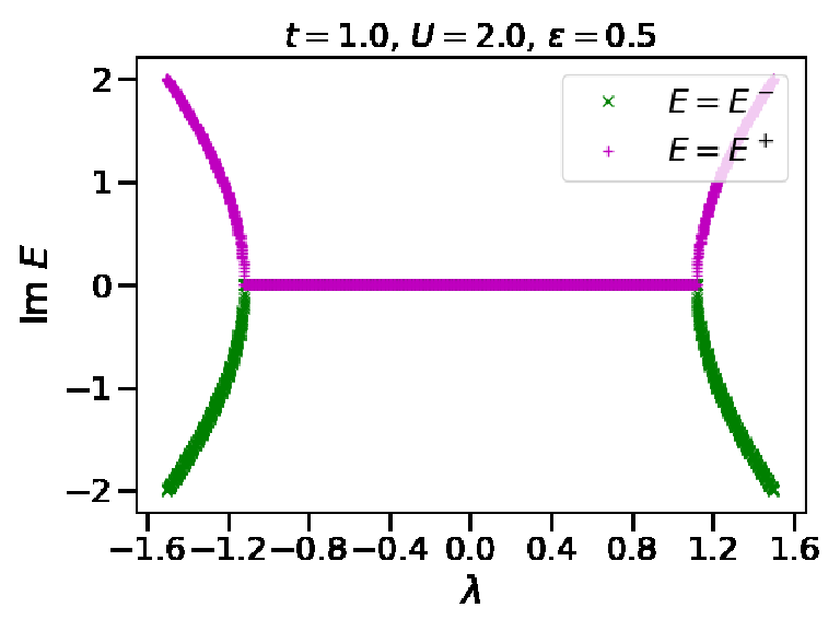
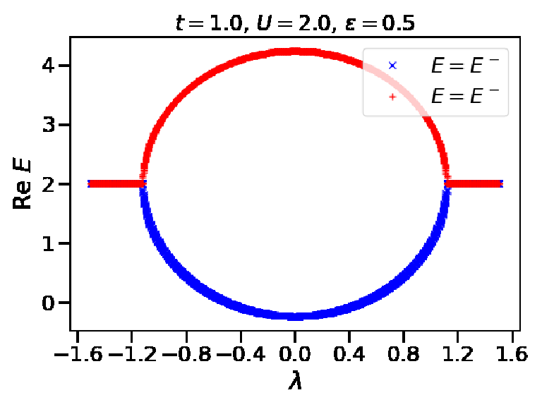
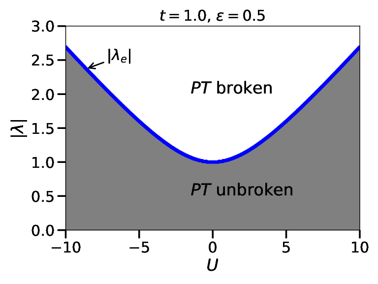
Thus the eigenenergies of $\hat{H}^{2}$ are $2\epsilon$ (degeneracy 3), $2\epsilon+U$, $\frac{1}{2}(4\epsilon\pm\sqrt{16t_{+}t_{-}+U^{2}}+U)=\frac{1}{2}(4\epsilon\pm\sqrt{16(t^{2}-\lambda^{2})+U^{2}}+U)$. We can check that by setting $U=0$ in Eq. (37), we get back the non-interacting limit (Eq. (26)). We have complex eigenenergies when the discriminant (term inside the square root) becomes negative, i.e. when $|\lambda|>\sqrt{t^{2}+U^{2}/16}$. Thus presence of interaction shifts the positions of the EPs and we have $\lambda_{e}=\pm\sqrt{t^{2}+U^{2}/16}$, agreeing with the recently studied Hubbard dimer model with entirely complex hopping ($t=0$) [18]. For our choice of parameters: $t=1$, $U=2$, $\epsilon=0.5$, we find $\lambda_{e}\simeq\pm 1.118$ (see Fig. 2(a) and Fig. 2(b) for the imaginary and real parts of $E^{\pm}$). Fig. 2(c) shows $\lambda_{e}$ symmetrically shifts from the non-interacting limit ($\lambda_{e}(U=0)=1$) as $U$ moves both in positive and negative directions. The presence of finite Coulomb interaction tends to localize electrons, reduces the kinetic energy of the electrons (all kinds of hopping) and prevents the system from encountering the dynamic instability. Thus finite $U$ eventually delays the PT-breaking transition and we notice minimum $|\lambda_{e}|$ at $U=0$. The parabolic curve for $|\lambda_{e}|$ marks the boundary between $\mathscr{PT}$ broken and unbroken phases on the $|\lambda|-U$ plane.

We now consider the case when the orbital energies of the hydrogen atoms get tuned to different energy levels by addition of complex loss and gain terms. For simplicity, let $\epsilon_{+}=\epsilon+i\gamma$, $\epsilon_{-}=\epsilon-i\gamma$ be the energies, i.e. there are equal amounts of loss and gain terms added to the orbital energies. Hence the orbital part of our Hamiltonian becomes

$\displaystyle\hat{H}^{\gamma}=\epsilon_{+}\sum_{\sigma}c^{{\dagger}}_{1\sigma}c^{\phantom{{\dagger}}}_{1\sigma}+\epsilon_{-}\sum_{\sigma}c^{{\dagger}}_{2\sigma}c^{\phantom{{\dagger}}}_{2\sigma}\,.$

(38)

Two-level or two-band systems with loss and gain terms have been successfully realized in several photonic and optical setups [39, 40, 7, 41, 42]. Considering both diagonal and off-diagonal non-Hermiticity, our most generic $\mathscr{PT}$ symmetric Hamiltonian reads

	$\displaystyle\hat{H}^{3}$	$\displaystyle=H^{\lambda}+H^{\gamma}+H^{U}$
		$\displaystyle=\sum_{\sigma}\big[\epsilon_{+}c^{{\dagger}}_{1\sigma}c^{\phantom{{\dagger}}}_{1\sigma}+\epsilon_{-}c^{{\dagger}}_{2\sigma}c^{\phantom{{\dagger}}}_{2\sigma}+t_{+}c^{{\dagger}}_{1\sigma}c^{\phantom{{\dagger}}}_{2\sigma}+t_{-}c^{{\dagger}}_{2\sigma}c^{\phantom{{\dagger}}}_{1\sigma}\big]$
		$\displaystyle\quad+U(\hat{n}_{1\uparrow}\hat{n}_{1\downarrow}+\hat{n}_{2\uparrow}\hat{n}_{2\downarrow})\,.$		(39)

$\mathscr{PT}$ symmetric non-Hermitian physics have been successfully observed in several two level photonic and optical systems [49]. One particular feature of such Hamiltonians is the existence of exceptional points (EPs) beyond which complex eigenenergies emerge signaling breaking of the symmetry in the eigenfunctions. As a simplistic model, we consider a hydrogen molecule with Hubbard interaction acting between its atoms’ electrons. We then introduce both diagonal and off-diagonal non-Hermitian terms to the Hamiltonian preserving its $\mathscr{PT}$ symmetry. Though effects of diagonal and off-diagonal terms have been studied extensively in the past, however, discussions on their dual presence in the same Hamiltonian is surprisingly missing in the literature, specifically with a particle-particle interaction term. Our work fills up this fundamental gap.

In our model, the $\mathscr{PT}$-symmetry broken phases occur due to competitions among several energy scales, mainly $t$, $U$, $\lambda$, and $\gamma$ (in our treatment, the orbital energy $\epsilon$ is a reference scale which can be set to zero or any constant value without loss of generality). $t$ and $U$ constitute the Hermitian terms, however, they compete against each other and take off-diagonal and diagonal positions respectively in the Hamiltonian matrix. Like in any $\mathscr{PT}$-symmetric Hamiltonian, both non-Hermiticity parameters $\lambda$ and $\gamma$ compete with the Hermitian $t$-term and spontaneously break the $\mathscr{PT}$-symmetry when the eigenenergies become complex (terms inside the square root becomes negative). The eigenenergy plots for both parameters are similar and follow the generic two-level state (TLS)’s $\mathscr{PT}$-symmetric diagrams. However, the presence of Hubbard interaction $U$ destroys the similarity between $\lambda$ and $\gamma$ and gives rise to a complicated cubic equation, which generically can have two complex roots in the broken symmetry regime. It is the nature of the Hubbard interaction and fermionic operators that gives rise to the $6\times 6$ matrix (Eq. (42)) which reduces to a cubic characteristic equation (for $U\neq 0$) instead of a typical TLS-type quadratic one. The physical understanding of this scenario could be the following. In the absence of interaction and off-diagonal non-Hermiticity $\lambda$, $\gamma$-term has to compete with the symmetric hopping $t$ only. Hence $U=0$ places the $\mathscr{PT}$-breaking boundary at the hopping amplitude: $|\gamma_{e}|=t$ (Fig. 6(a)). In the TLS language, $t$ induces avoided level crossing while $\gamma$ encourages crossing or transition between two energy levels [17]. Since Hubbard interaction $U$ goes against the kinetic term $t$, the term eventually enhances the effect of $\gamma$ (dissociation of the $H_{2}$ molecule) [17]. Thus we see $|\gamma_{e}|$ monotonically decreasing as $U$’s value rises. Now finite $\lambda$ joins hands with $\gamma$ and together lead to dynamical instability, hence $PT$-boundary gets reduced in the presence of finite $\lambda$ (Fig. 6(a)). It is worth mentioning that recently Pan and coworkers [23]] studied the Hubbard dimer model using the Lindblad master equation and found that the rescaled probability diverges at the same threshold value of interaction strength as found in the $\mathscr{PT}$-breaking effective non-Hermitian Hubbard dimer Hamiltonian.

We notice that interaction plays differently with different kinds of EPs generated by the parameters of the Hamiltonian. Changing the position of one kind of EPs in the increasing direction and the other kind in decreasing direction by varying interaction strength can offer flexibility in fine tuning EPs and more control over their potential applications. In a realistic hydrogen molecule, non-Hermitian loss-gain terms might be introduced through laser induced molecular ionization and dissociation [16, 17]. Besides this, a more precise two-site Hubbard model could be emulated in an ultracold double well system [50] or via NMR [51]. The role of Hubbard interaction on the EPs has been studied recently [23]. However, the interplay of the diagonal and off-diagonal $\mathscr{PT}$-symmetries and the role of interaction on them have not been studied ever to the best of our knowledge. Such interplay might be extended to the fermionic or bosonic lattice Hubbard models and effect on interesting physics such as closure of Mott gap [15, 22, 52] or multiple $\mathscr{PT}$-broken phases [53] can be studied. Finally, we must mention that the cube-root based EPs, found in our simplistic model, may require deeper understanding with potential applications in various areas of physics and quantum chemistry.

The authors thank the HBCSE, Mumbai, for providing an opportunity to collaborate through their NIUS Physics 15.3 camp. HB is indebted to Vikram Tripathi, TIFR, Mumbai, for several useful discussions and his valuable inputs.

Our codes are available on the Github repository:
https://github.com/hbaromega/PT-symmetric-2-site-Hubbard-hydrogen,
under GNU General Public License.

References

- [1] Carl M. Bender and Stefan Boettcher. Real spectra in non-hermitian hamiltonians having symmetry. Phys. Rev. Lett., 80:5243–5246, Jun 1998.
- [2] Nathan R. Bernier, Emanuele G. Dalla Torre, and Eugene Demler. Unstable avoided crossing in coupled spinor condensates. Phys. Rev. Lett., 113:065303, Aug 2014.
- [3] Zin Lin, Hamidreza Ramezani, Toni Eichelkraut, Tsampikos Kottos, Hui Cao, and Demetrios N. Christodoulides. Unidirectional invisibility induced by -symmetric periodic structures. Phys. Rev. Lett., 106:213901, May 2011.
- [4] Alois Regensburger, Christoph Bersch, Mohammad-Ali Miri, Georgy Onishchukov, Demetrios N. Christodoulides, and Ulf Peschel. Parity–time synthetic photonic lattices. Nature, 488(7410):167–171, Aug 2012.
- [5] Xuefeng Zhu, Liang Feng, Peng Zhang, Xiaobo Yin, and Xiang Zhang. One-way invisible cloak using parity-time symmetric transformation optics. Opt. Lett., 38(15):2821–2824, Aug 2013.
- [6] Liang Feng, Ye-Long Xu, William S. Fegadolli, Ming-Hui Lu, José E. B. Oliveira, Vilson R. Almeida, Yan-Feng Chen, and Axel Scherer. Experimental demonstration of a unidirectional reflectionless parity-time metamaterial at optical frequencies. Nature Materials, 12(2):108–113, Feb 2013.
- [7] A. Guo, G. J. Salamo, D. Duchesne, R. Morandotti, M. Volatier-Ravat, V. Aimez, G. A. Siviloglou, and D. N. Christodoulides. Observation of -symmetry breaking in complex optical potentials. Phys. Rev. Lett., 103:093902, Aug 2009.
- [8] Qingjie Liu, Jibing Liu, Dong Zhao, and Bing Wang. On-chip experiment for chiral mode transfer without enclosing an exceptional point. Phys. Rev. A, 103:023531, Feb 2021.
- [9] Linlin Geng, Weixuan Zhang, Xiangdong Zhang, and Xiaoming Zhou. Topological mode switching in modulated structures with dynamic encircling of an exceptional point. Proceedings of the Royal Society A: Mathematical, Physical and Engineering Sciences, 477(2245):20200766, 2021.
- [10] Hossein Hodaei, Mohammad-Ali Miri, Matthias Heinrich, Demetrios N. Christodoulides, and Mercedeh Khajavikhan. Parity-time–symmetric microring lasers. Science, 346(6212):975–978, 2014.
- [11] Liang Feng, Zi Jing Wong, Ren-Min Ma, Yuan Wang, and Xiang Zhang. Single-mode laser by parity-time symmetry breaking. Science, 346(6212):972–975, 2014.
- [12] B. Peng et al. Parity–time-symmetric whispering-gallery microcavities. Nature Phys, 10:394–398, 2014.
- [13] Jan Wiersig. Enhancing the sensitivity of frequency and energy splitting detection by using exceptional points: Application to microcavity sensors for single-particle detection. Phys. Rev. Lett., 112:203901, May 2014.
- [14] H. Hodaei, A. Hassan, S. Wittek, et al. Enhanced sensitivity at higher-order exceptional points. Nature, 548:187–191, 2017.
- [15] Vikram Tripathi, Alexey Galda, Himadri Barman, and Valerii M. Vinokur. Parity-time symmetry-breaking mechanism of dynamic mott transitions in dissipative systems. Phys. Rev. B, 94:041104, Jul 2016.
- [16] R. Lefebvre, O. Atabek, M. Šindelka, and N. Moiseyev. Resonance coalescence in molecular photodissociation. Phys. Rev. Lett., 103:123003, Sep 2009.
- [17] I. A. Wrona, M. W. Jarosik, R. Szczȩśniak, K. A. Szewczyk, M. K. Stala, and W. Leoński. Interaction of the hydrogen molecule with the environment: stability of the system and the pt symmetry breaking. Scientific Reports, 10(1):215, Jan 2020.
- [18] Antoine Marie, Hugh G A Burton, and Pierre-François Loos. Perturbation theory in the complex plane: exceptional points and where to find them. J. Phys.: Condens. Matter, 2021.
- [19] Yuto Ashida, Shunsuke Furukawa, and Masahito Ueda. Parity-time-symmetric quantum critical phenomena. Nature Communications, 8(1):15791, Jun 2017.
- [20] José A. S. Lourenço, Ronivon L. Eneias, and Rodrigo G. Pereira. Kondo effect in a -symmetric non-hermitian hamiltonian. Phys. Rev. B, 98:085126, Aug 2018.
- [21] Tsuneya Yoshida, Robert Peters, Norio Kawakami, and Yasuhiro Hatsugai. Symmetry-protected exceptional rings in two-dimensional correlated systems with chiral symmetry. Phys. Rev. B, 99:121101, Mar 2019.
- [22] V. Tripathi and V. M. Vinokur. Pt-symmetric effective model for nonequilibrium phase transitions in a dissipative fermionic mott insulator chain. Scientific Reports, 10(1):7304, Apr 2020.
- [23] Lei Pan, Xueliang Wang, Xiaoling Cui, and Shu Chen. Interaction-induced dynamical -symmetry breaking in dissipative fermi-hubbard models. Phys. Rev. A, 102:023306, Aug 2020.
- [24] Cheng Chin, Rudolf Grimm, Paul Julienne, and Eite Tiesinga. Feshbach resonances in ultracold gases. Rev. Mod. Phys., 82:1225–1286, Apr 2010.
- [25] Yosuke Takasu, Tomoya Yagami, Yuto Ashida, Ryusuke Hamazaki, Yoshihito Kuno, and Yoshiro Takahashi. PT-symmetric non-Hermitian quantum many-body system using ultracold atoms in an optical lattice with controlled dissipation. Progress of Theoretical and Experimental Physics, 2020(12), 09 2020. 12A110.
- [26] R.P. Feynman, R.B. Leighton, and M. Sands. The Feynman Lectures on Physics. Number v. 3 in Addison-Wesley world student series. Addison-Wesley, 1977.
- [27] Jan R. Rubbmark, Michael M. Kash, Michael G. Littman, and Daniel Kleppner. Dynamical effects at avoided level crossings: A study of the landau-zener effect using rydberg atoms. Phys. Rev. A, 23:3107–3117, Jun 1981.
- [28] S.N. Shevchenko, S. Ashhab, and Franco Nori. Landau–zener–stückelberg interferometry. Physics Reports, 492(1):1–30, 2010.
- [29] Qing-hai Wang. 2 x 2 pt-symmetric matrices and their applications. Philosophical Transactions of the Royal Society A: Mathematical, Physical and Engineering Sciences, 371(1989):20120045, 2013.
- [30] A.N. W, N.W. Ashcroft, N.D. Mermin, N.D. Mermin, and Brooks/Cole Publishing Company. Solid State Physics. HRW international editions. Holt, Rinehart and Winston, 1976.
- [31] B Alvarez-Fernandez and J A Blanco. The hubbard model for the hydrogen molecule. European Journal of Physics, 23(1):11–16, nov 2001.
- [32] William R. Frensley. Boundary conditions for open quantum systems driven far from equilibrium. Rev. Mod. Phys., 62:745–791, Jul 1990.
- [33] Jean Dalibard, Yvan Castin, and Klaus Mølmer. Wave-function approach to dissipative processes in quantum optics. Phys. Rev. Lett., 68:580–583, Feb 1992.
- [34] Naomichi Hatano and David R. Nelson. Localization transitions in non-hermitian quantum mechanics. Phys. Rev. Lett., 77:570–573, Jul 1996.
- [35] Takahiro Fukui and Norio Kawakami. Breakdown of the mott insulator: Exact solution of an asymmetric hubbard model. Phys. Rev. B, 58:16051–16056, Dec 1998.
- [36] Reinhold A. Bertlmann, Walter Grimus, and Beatrix C. Hiesmayr. Open-quantum-system formulation of particle decay. Phys. Rev. A, 73:054101, May 2006.
- [37] D. Cabib. Electrical conductivity of the narrow-half-filled-band hubbard model with nearest-neighbor interaction. Phys. Rev. B, 12:2189–2193, Sep 1975.
- [38] F. Gebhard. The Mott Metal-Insulator Transition: Models and Methods. Springer Tracts in Modern Physics. Springer Berlin Heidelberg, 2010.
- [39] E. Persson, I. Rotter, H.-J. Stöckmann, and M. Barth. Observation of resonance trapping in an open microwave cavity. Phys. Rev. Lett., 85:2478–2481, Sep 2000.
- [40] K. G. Makris, R. El-Ganainy, D. N. Christodoulides, and Z. H. Musslimani. Beam dynamics in symmetric optical lattices. Phys. Rev. Lett., 100:103904, Mar 2008.
- [41] L. Feng, R. El-Ganainy, and L. Ge. Non-hermitian photonics based on parity–time symmetry. Nature Photon, 11:752–762, 2017.
- [42] C Li, P Wang, L Jin, and Z Song. An attractor dynamics in a non-hermitian two-level system. Journal of Physics Communications, 5(10):105011, oct 2021.
- [43] J.P. Tignol. Galois’ Theory of Algebraic Equations. World Scientific, 2001.
- [44] W.H. Press, W.H. Press, S.A. Teukolsky, W.T. Vetterling, W.T. Vetterling, B.P. Flannery, and B.P. Flannery. Numerical Recipes in C++: The Art of Scientific Computing. Cambridge University Press, 2002.
- [45] Bo Zhen, Chia Wei Hsu, Yuichi Igarashi, Ling Lu, Ido Kaminer, Adi Pick, Song-Liang Chua, John D. Joannopoulos, and Marin Soljačić. Spawning rings of exceptional points out of dirac cones. Nature, 525(7569):354–358, Sep 2015.
- [46] Tao Liu, James Jun He, Zhongmin Yang, and Franco Nori. Higher-order weyl-exceptional-ring semimetals. Phys. Rev. Lett., 127:196801, Nov 2021.
- [47] Rainer Strack and Dieter Vollhardt. Hubbard model with nearest-neighbor and bond-charge interaction: Exact ground-state solution in a wide range of parameters. Phys. Rev. Lett., 70:2637–2640, Apr 1993.
- [48] E. G. C. P. van Loon, M. Schüler, M. I. Katsnelson, and T. O. Wehling. Capturing nonlocal interaction effects in the hubbard model: Optimal mappings and limits of applicability. Phys. Rev. B, 94:165141, Oct 2016.
- [49] C.M. Bender. Pt Symmetry: In Quantum And Classical Physics. World Scientific Publishing Company, 2018.
- [50] Simon Murmann, Andrea Bergschneider, Vincent M. Klinkhamer, Gerhard Zürn, Thomas Lompe, and Selim Jochim. Two fermions in a double well: Exploring a fundamental building block of the hubbard model. Phys. Rev. Lett., 114:080402, Feb 2015.
- [51] Filipe V. Melo, Alexandre M. Souza, Ivan S. Oliveira, and Roberto S. Sarthour. Quantum simulation of the two-site hubbard hamiltonian. Physics Open, 6:100053, 2021.
- [52] Roman Rausch, Robert Peters, and Tsuneya Yoshida. Exceptional points in the one-dimensional hubbard model. New J. Phys., 23(1):013011, jan 2021.
- [53] L. Jin and Z. Song. Scaling behavior and phase diagram of a pt-symmetric non-hermitian bose–hubbard system. Annals of Physics, 330:142–159, 2013.