Stack-Sorting for Coxeter Groups
Abstract.
Given an essential semilattice congruence on the left weak order of a Coxeter group , we define the Coxeter stack-sorting operator by , where is the unique minimal element of the congruence class of containing . When is the sylvester congruence on the symmetric group , the operator is West’s stack-sorting map. When is the descent congruence on , the operator is the pop-stack-sorting map. We establish several general results about Coxeter stack-sorting operators, especially those acting on symmetric groups. For example, we prove that if is an essential lattice congruence on , then every permutation in the image of has at most right descents; we also show that this bound is tight.
We then introduce analogues of permutree congruences in types and and use them to isolate Coxeter stack-sorting operators and that serve as canonical type- and type- counterparts of West’s stack-sorting map. We prove analogues of many known results about West’s stack-sorting map for the new operators and . For example, in type , we obtain an analogue of Zeilberger’s classical formula for the number of -stack-sortable permutations in .
1. Introduction
1.1. Coxeter Stack-Sorting Operators
A semilattice congruence on a meet-semilattice is an equivalence relation on that respects meets. More precisely, this means that if and , then . If has a minimal element and is locally finite, then every congruence class of has a unique minimal element, and we denote by the projection map that sends each element of to the unique minimal element of its congruence class. We omit the superscript and write when the congruence is clear from context. If is a lattice, then a lattice congruence on is an equivalence relation on that respects both meets and joins, meaning and together imply and .
Let be a Coxeter system, and let and denote, respectively, the left and right weak orders on . The posets and are isomorphic to each other, and a foundational theorem due to Björner [8] states that they are complete meet-semilattices. We write for the meet of two elements in the left weak order. If is finite, then the left and right weak orders on are lattices; in this case, we write for the join of and in the left weak order.
Semilattice congruences and lattice congruences on weak orders of Coxeter groups have been studied extensively [2, 17, 45, 47, 44, 39, 34, 37, 49, 51, 52, 54, 55, 56, 57, 58, 59], especially due to their strong connections with polyhedral geometry, Hopf algebras, and cluster algebras. One of the quintessential examples of a lattice congruence is provided by the sylvester congruence on the symmetric group [36], which is closely related to Tamari lattices, associahedra, and the Hopf algebra of binary plane trees [40, 41]; we define this congruence in Section 6. The sylvester congruence is the prototypical example of a Cambrian congruence [49, 54, 55, 56, 57, 58, 59]. Other notable lattice congruences on symmetric groups are the permutree congruences [45], the -twist congruences [44], and the Baxter congruences [39, 34].
Another important semilattice congruence, which is defined on an arbitrary Coxeter group , is the descent congruence, which we denote by . Two elements of are equivalent in the descent congruence if and only if they have the same right descent set. The descent congruence on the symmetric group provides one of the other primary motivating examples of a permutree congruence besides the sylvester congruence.
A semilattice congruence on the left weak order of is called essential11 1 As discussed in [2, 37, 47, 51], lattice congruences of symmetric groups give rise to fans called quotient fans. A lattice congruence on is essential if and only if the corresponding quotient fan is essential. if the identity element belongs to a singleton congruence class.
Definition 1.1.
Let be a Coxeter system, and let be an essential semilattice congruence on the left weak order of . Define the Coxeter stack-sorting operator to be the map given by for all .
The motivation for the name Coxeter stack-sorting operator comes from two special cases. First, when is the symmetric group and is the sylvester congruence, the map is West’s stack-sorting map. Indeed, this is the content of [25, Corollary 16] (where the map goes by the name swd), and it is also a special case of Proposition 6.4 below. This map was originally defined by West [63] as a deterministic variant of a stack-sorting machine introduced by Knuth [38]. West’s stack-sorting map, which we will often simply call the stack-sorting map, has now received vigorous attention and has found connections with several other parts of combinatorics [10, 12, 11, 13, 28, 22, 21, 25, 23, 29, 35, 42, 60, 64, 33]. The second motivation for our terminology comes from the fact that when is the descent congruence on , the map is the pop-stack-sorting map. This function, which is a deterministic analogue of a pop-stack-sorting machine introduced by Avis and Newborn in [5], first appeared in a paper of Ungar’s about directions determined by points in the plane [62]; it has received a great deal of attention over the past few years [1, 3, 4, 26, 32, 18, 19, 48].
Remark 1.2.
In order to earn the title of sorting operator, a map better have the property that for every , there is some such that . This is precisely why we require to be essential in Definition 1.1. Indeed, if we allowed for the case where for some , then would be a fixed point of . ∎
Remark 1.3.
The authors of the recent paper [15] introduced a different generalization of West’s stack-sorting map that uses pattern-avoiding stacks; this notion has spawned several subsequent articles in recent years [6, 7, 14, 16, 30]. While these pattern-avoiding stacks are certainly interesting, we believe our Coxeter stack-sorting operators are more natural from an algebraic and lattice-theoretic point of view.
The recent article [46] also generalizes stack-sorting to the realm of permutrees. However, the approach and the results in that paper are quite different from ours. ∎
Remark 1.4.
The downward projection map is crucial when is a Cambrian congruence on a Coxeter group because its image is the set of sortable elements [54, 58, 59]. Although Reading originally named these elements sortable because of the connection with West’s stack-sorting map and Knuth’s stack-sorting machine, he did not study Coxeter stack-sorting operators. For an arbitrary semilattice congruence on , the elements of the image of can still be called the sortable elements in our setting because they are the elements of that get sorted into the identity after only a single application of . ∎
In [26], the author investigated the Coxeter stack-sorting operators corresponding to descent congruences on Coxeter groups, which were called Coxeter pop-stack-sorting operators. Our goal in this paper is to initiate the investigation of Coxeter stack-sorting operators more generally and to consider specific Coxeter stack-sorting operators that are more closely related to West’s stack-sorting map.
1.2. Outline
In order to motivate many of our results, it is helpful to discuss previous work on West’s stack-sorting map. We do this in Section 2, where we simultaneously present a more thorough synopsis of our main theorems from Sections 5, 7, and 8 than what we give here. Section 3 summarizes some basic facts and terminology related to Coxeter groups that we will need later. In Section 4, we establish results that hold for arbitrary Coxeter stack-sorting operators. For example, we will prove that the statistic that keeps track of the number of preimages of an element of under is a decreasing function on the left weak order. Section 5 investigates the maximum number of right descents that a permutation in in the image of a Coxeter stack-sorting operator can have. In Section 6, we discuss permutrees and permutree congruences, and we show that Coxeter stack-sorting operators associated to permutree congruences can be described in terms of postorder readings of decreasing permutrees. This provides a useful combinatorial model for dealing with these permutree stack-sorting operators. In Section 7, we introduce analogues of permutrees and permutree congruences for the hyperoctahedral groups . One specific type- permutree congruence on , which we call the type- sylvester congruence, yields a Coxeter stack-sorting operator that can be seen as the canonical type- analogue of West’s stack-sorting map; much of Section 7 is devoted to studying this operator. In Section 8, we introduce analogues of permutrees and permutree congruences for the affine symmetric groups . One specific choice of an affine permutree congruence on , which we call the affine sylvester congruence, yields a Coxeter stack-sorting operator that serves as a canonical type- analogue of West’s stack-sorting map; a large portion of Section 8 concerns this operator. Finally, Section 9 lists several suggestions for potential future work.
2. West’s Stack-Sorting Map
In this paper, a permutation of size is a bijection for some -element set . We write permutations as words in one-line notation. The symmetric group is the set of permutations of the set . The standardization of a permutation of size is the permutation in obtained by replacing the -smallest entry in with for all . For example, is a permutation of size whose standardization is .
Let denote West’s stack-sorting map. A simple recursive definition of is as follows. First, define , where is the empty permutation. Given a nonempty permutation with largest entry , we can write in one-line notation as . Then define to be . For example,
We say a permutation is -stack-sortable if is an increasing permutation. It follows from Knuth’s analysis [38] that a permutation is -stack-sortable if and only if it avoids the pattern ; Knuth also showed that the number of -avoiding permutations in is the Catalan number (see [10, Chapters 4 and 8]). There has been a great deal of work dedicated to understanding -stack-sortable permutations (see [10, 12, 11, 13, 28, 22, 35, 64, 33] and the references therein); the first major result proved about these permutations was Zeilberger’s theorem, which states that the number of -stack-sortable permutations in is [64]. Úlfarsson characterized -stack-sortable permutations [61]; only recently were these permutations enumerated via a complicated recurrence relation [22].
Consider the affine symmetric group , as defined in Section 8. We will introduce a specific Coxeter stack-sorting operator . Let us say an affine permutation is -stack-sortable if . In Section 8, we will see that -stack-sortable affine permutations are also characterized by the property of avoiding the pattern . A theorem due to Crites [20] states that the number of -avoiding affine permutations in is . We will enumerate -stack-sortable affine permutations, thereby obtaining an affine analogue of Zeilberger’s seminal formula. To be more precise, let us write for the set of -stack-sortable elements of , and let and . We will prove that
Given a set , a function , and an element , we define the forward orbit of under to be the set . When confronted with such a dynamical system, it is natural to consider the sizes of the forward orbits, and it is particularly natural to ask for . Additional motivation for studying this quantity when is a sorting operator comes from the observation that it measures the worst-case complexity of the sorting procedure. West [63] proved that is , which happens to be the Coxeter number of . In Section 4, we invoke a theorem from [26] to see that if is an arbitrary finite irreducible Coxeter group and , then the size of the forward orbit of under a Coxeter stack-sorting operator is at most the Coxeter number of . It follows that every forward orbit of the specific map that we define in Section 7 has size at most the Coxeter number of , which is . However, we improve this estimate in Section 7, showing that
If , then the number of right descents of is at most (see [29] and [10, Chapter 8, Exercise 18]). This result is natural if one thinks of the stack-sorting map as a genuine sorting procedure and views the number of right descents of a permutation in as a measure of how “far away” the permutation is from being sorted into the identity. In Section 5, we prove that a similar result completely fails for arbitrary Coxeter stack-sorting operators on symmetric groups. Namely, we show that for each , there exist a permutation and an essential semilattice congruence on such that has right descents. However, we will see that there is a nontrivial upper bound on the number of right descents when we restrict our attention to lattice congruences. We prove that if is an essential lattice congruence on , then every permutation in the image of has at most right descents. Moreover, we will see that this bound is tight because it is attained when is the descent congruence. In Section 7, we find that the maximum number of right descents that an element of in the image of can have is . In Section 8, we prove that the maximum number of right descents that an element of in the image of can have is also .
The number of preimages of a permutation under the stack-sorting map is called the fertility of . In [25], the author proved that the fertility of only depends on the sylvester class of . An analogous result fails for arbitrary Coxeter stack-sorting operators, but we will see that it does hold for , the affine analogue of the stack-sorting map. Define the fertility of an element to be . We will see that the fertility of is finite and only depends on the affine sylvester class of . (The affine sylvester congruence is the semilattice congruence used to define .) In fact, we will prove that for every , the number of preimages of under is finite and only depends on the affine sylvester class of .
In [29], Engen, Miller, and the present author defined a permutation to be uniquely sorted if its fertility is . They proved the following characterization of these permutations.
Proposition 2.1 ([29]).
Let . A permutation of size is uniquely sorted if and only if it is in the image of the stack-sorting map and has exactly descents. In particular, there are no uniquely sorted permutations of size if is even.
Quite surprisingly, uniquely sorted permutations are counted by a fascinating sequence called Lassalle’s sequence (sequence A180874 in [43]), which is the sequence of absolute values of the classical cumulants of the standard semicircular distribution [29]. Uniquely sorted permutations also possess several other remarkable enumerative properties [29, 21, 42, 60].
Let us say an affine permutation is uniquely sorted if its fertility is . We prove in Section 8 that an element of is uniquely sorted if and only if it is in the image of and has exactly right descents. In particular, there are no uniquely sorted affine permutations in when is odd. When is even, there are infinitely many uniquely sorted elements of . Because we know (by Theorem 7.3) that the fertility of an element of only depends on its affine sylvester class, it is natural to define an affine sylvester class in to be uniquely sorted if its elements are uniquely sorted. We prove that the number of uniquely sorted affine sylvester classes in is
This appears to be the first combinatorial interpretation for these numbers, which form sequence A107026 in [43].
Much of the author’s work on the stack-sorting map has relied on a certain Decomposition Lemma, which provides a recursive method for computing the fertility of a permutation, and a certain Fertility Formula, which gives an explicit expression for the fertility of a permutation as a sum over combinatorial objects called valid hook configurations. These tools have led to several new results about the stack-sorting map, including the aforementioned recurrence for counting -stack-sortable permutations [22], theorems about uniquely sorted permutations [29, 21, 42, 60], a very surprising and useful connection with cumulants in noncommutative probability theory [28], and connections with certain polytopes called nestohedra [23]. In Section 8, we introduce affine valid hook configurations, and we prove analogues of the Decomposition Lemma and the Fertility Formula for affine permutations. These tools are what allow us to enumerate uniquely sorted affine sylvester classes.
3. Coxeter Groups
We assume basic familiarity with the combinatorics of Coxeter groups; a standard reference for the subject is [9]. We will often refer to a Coxeter group with the understanding that we are really referring to a Coxeter system for some specific set of simple generators. We let denote the identity element of . Thus, has a presentation of the form such that for all and for all distinct . The length of an element , denoted , is the length of a reduced word for . The left weak order on is the partial order on defined by saying if . The right weak order on is the partial order on defined by saying if . The map given by is an isomorphism from the left weak order to the right weak order. A right descent of an element is a simple generator such that ; the collection of all right descents of is the right descent set of , which we denote by . Equivalently, . A Coxeter element of a finite Coxeter group is an element obtained by multiplying the simple generators together in some order; all Coxeter elements have the same order in , which is called the Coxeter number of . A Coxeter group is called irreducible if its Coxeter diagram is a connected graph.
The Coxeter groups of type are the symmetric groups . The elements of are permutations of , which we write as words in one-line notation. The simple generators of are , where is the transposition that swaps and . The transposition is a right descent of a permutation if and only if . A right inversion (respectively, left inversion) of is a pair such that and (respectively, ). For , we have (respectively, ) if and only if every right (respectively, left) inversion of is a right (respectively, left) inversion of . The number of right (equivalently, left) inversions of is .
Recall that, in this article, a permutation of size is a bijection , where has cardinality . The one-line notation of is the word . The plot of is the diagram showing the points for all . It is often convenient to consider plots modulo horizontal translation. In other words, moving all points in the plot of to the right or left by some fixed distance gives another diagram that we still call the plot of . We write for the set of indices such that ; such indices are called the descents of . We have if and only if .
We will often make use of the automorphism of the group defined by , where is the longest element of . The one-line notation of is
The plot of is obtained by rotating the plot of by . It is well known that is a lattice automorphism of the left (and also the right) weak order on . Therefore, given a semilattice congruence on , we can consider the semilattice congruence defined by saying if and only if . For all , we have
| (1) |
4. General Results
In this section, we collect some general facts about arbitrary Coxeter stack-sorting operators.
We first address the problem of determining the maximum size of a forward orbit of a Coxeter stack-sorting operator when is a finite irreducible Coxeter group. Recall from Remark 1.2 that our definition of a Coxeter stack-sorting operator guarantees that every forward orbit of contains , which is a fixed point. Thus, we will be concerned with the maximum number of iterations of needed to send an element to the identity.
Let be an arbitrary Coxeter group. In [26], the author defined a map to be compulsive if and for all and all . He proved that if is finite and irreducible and is compulsive, then , where is the Coxeter number of . We will see that Coxeter stack-sorting operators are compulsive. First, we need a simple lemma that gives an alternative characterization of essential semilattice congruences. Recall that an equivalence relation is said to refine an equivalence relation if every equivalence class of is contained in an equivalence class of .
Lemma 4.1.
A semilattice congruence on the left weak order of a Coxeter group is essential if and only if it refines the descent congruence on .
Proof.
Every refinement of the descent congruence is certainly essential because is the only element of with an empty right descent set. For the converse, suppose is an essential semilattice congruence on the left weak order of . Let be the set of simple generators of . Consider such that . Let . Because is a semilattice congruence, we have . Both and are less than or equal to in the left weak order, so they must belong to . Since , we deduce that . Therefore, if and only if . In other words, if and only if . As this is true for all , we conclude that , meaning . ∎
Proposition 4.2.
Let be an essential semilattice congruence on the left weak order of a Coxeter group . The Coxeter stack-sorting operator is compulsive. If is finite and irreducible and has Coxeter number , then
Proof.
To prove that is compulsive, we must prove that for every and . Fix such elements and . Let be the downward projection map associated to . Because , it follows from Lemma 4.1 that . Since , we have and . We know that and , so . Hence,
This shows that , completing the proof that is compulsive. The last statement in the theorem follows from Theorem 1.4 in [26]. ∎
The Coxeter number of is . Therefore, Proposition 4.2 states that if is a Coxeter stack-sorting operator on , then for all .
In [10, Chapter 8, Exercise 23], Bóna asks the reader to find the permutation in that has the maximum number of preimages under the stack-sorting map. As one might expect, the answer is the identity permutation . The number of preimages of under the stack-sorting map is the Catalan number , and every other permutation in has strictly fewer than preimages. This result is a special case of the following proposition because the number of congruence classes of the sylvester congruence on is the number of binary plane trees with vertices, which is .
Proposition 4.3.
Let be an essential semilattice congruence on the left weak order of a Coxeter group . Let be the number of congruence classes of , and assume is finite. Then , and for every .
Proof.
The elements of are precisely the minimal elements of the congruence classes, so . Now consider . If , then , and we know that because is in a singleton congruence class. It follows that the map is an injection from into , so . ∎
One of the main results of [24] states that for all , with equality if and only if . In other words, this theorem says that the action of the stack-sorting map causes fertilities of permutations to increase monotonically. The analogous result fails for an arbitrary Coxeter stack-sorting operator, even if we restrict our attention to . For example, if is the pop-stack-sorting map on , then , but . Nonetheless, there is still a certain monotonicity result that holds for all Coxeter stack-sorting operators.
Theorem 4.4.
Let be a Coxeter group, and let be a Coxeter stack-sorting operator. If are such that , then .
Proof.
It suffices to prove the result when . In this case, we can write for some simple generator . Choose . We can write , where because . Then . Because is a semilattice congruence and , we have . Consequently, . If follows that
Hence, we have an injection given by . ∎
5. Descents After Coxeter Stack-Sorting in Symmetric Groups
Recall that we write for West’s stack-sorting map, which coincides with the Coxeter stack-sorting operator defined using the sylvester congruence.
In this section, we analyze Coxeter stack-sorting operators on symmetric groups. It is natural to use the number of right descents of a permutation as a measure of how “far away” is from the identity permutation. Given that a Coxeter stack-sorting operator on is called a sorting operator, we might hope that the permutations in its image would be somewhat “close” to the identity. For example,
| (2) |
for all (see [29] and [10, Chapter 8, Exercise 18]). Is something similar true for other Coxeter stack-sorting operators?
If we allow to be an arbitrary essential semilattice congruence on the left weak order of , then can be as large as , as we will see below in Theorem 5.2. However, it turns out that if we require to be a lattice congruence, then the inequality holds. We will also see that this bound is tight.
Given a poset and elements with , we write for , the closed interval in between and . A meet-semilattice is called locally finite if every one of its closed intervals is finite.
Lemma 5.1.
Let be a locally finite meet-semilattice with a minimal element , and let be such that . There exists a semilattice congruence on that has as a congruence class.
Proof.
Let us say an equivalence relation on is cheerful if the following two conditions hold:
- •
is an equivalence class of ;
- •
if , then is in a singleton equivalence class of .
We are going to construct a sequence of cheerful equivalence relations on . First, let be the equivalence relation whose equivalence classes are and the singleton sets for ; it is clear that is cheerful.
Now let , and suppose we have already constructed the cheerful equivalence relation . Define the relation by saying if and only if either or there exist with , , , and . Let be the transitive closure of . To see that is cheerful, we first need to show that is an equivalence class of . Notice that is certainly contained in an equivalence class of because it is an equivalence class of . Now suppose, by way of contradiction, that is properly contained in an equivalence class of . Then there exist and such that . We know that because is cheerful, so there must exist with , , , and . Observe that . If , then because is cheerful. In this case, , so , again because is cheerful. Similarly, if , then . Since , the elements and cannot both belong to . Thus, either or . Without loss of generality, assume . We know that because . Consequently, . We find that and , so . However, , and this contradicts the assumption that . Hence, is an equivalence class of .
Consider with . Suppose, by way of contradiction, that is not an equivalence class of . Then for some . We know that because is cheerful. Therefore, there exist with , , , and . Because , we have and . Since is cheerful, we must have and , so . This is a contradiction, so we deduce that is cheerful.
By induction, all of the equivalence relations are cheerful. The fact that is locally finite (in particular, is finite) implies that there is some such that and are identical. Thus, is the same as . It follows from our construction of from that is a semilattice congruence on . Because is cheerful, it has as a congruence class. ∎
A subset of a poset is called convex if for all , we have . A simple consequence of the definition of a semilattice congruence, which we will need in the proof of the next proposition, is that every congruence class of a semilattice congruence is convex.
Theorem 5.2.
For each , we have
where the first maximum is over all essential semilattice congruences on the left weak order of .
Proof.
It follows from Definition 1.1 that the decreasing permutation is not in the image of any Coxeter stack-sorting operator on . Therefore, .
Let . Define by for odd and for even. Define by for odd and for even. For example, when , we have and . One can readily verify that every right inversion of is a right inversion of , so . Moreover, , so . The congruence classes of are convex, so is contained in one such congruence class. The left weak order on a Coxeter group is locally finite and has as its unique minimal element. According to Lemma 5.1, there is a semilattice congruence on that has as a congruence class. Let be the common refinement of and . In other words, we define by declaring if and only if and . Then is an essential semilattice congruence on that has as a congruence class. Finally, is a permutation in the image of with right descents. ∎
Our next goal is to prove that permutations in the image of a Coxeter stack-sorting operator arising from a lattice congruence on must have at most right descents. To do this, we will make use of a combinatorial description of the lattice congruences on due to Reading. These concepts are discussed in more detail in [37, 53] and [50, Section 10-5], where they are formulated in terms of the right weak order on ; it is easy to translate to the left weak order by taking inverses of permutations.
Fix . Suppose is a cover relation in the left weak order on . Then for some . If we let and and let be the transposition that swaps and , then . Let (equivalently, ). We label the edge in the Hasse diagram of with the tuple . The fence associated to the tuple , denoted , is the set of all edges in the Hasse diagram of with label . Let
be the set of all such fences. The forcing order is the partial order on given by declaring whenever and . Figure 1 shows the four fences of the left weak order on and the corresponding forcing order.
For each lattice congruence on , let be the set of edges in the Hasse diagram of such that . Let be the collection of fences in that have a nonempty intersection with . In other words, is in if and only if there is an edge with label such that .
The following theorem appeared originally as [53, Theorem 4.6]; although, in [37, Theorem 4], it was reformulated in a manner closer to what we have presented.
Theorem 5.3 ([53]).
If is a lattice congruence on , then . Furthermore, the map is a bijection from the set of lattice congruences on to the set of order ideals of .
The following lemma will handle most of the heavy lifting in our proof of Theorem 5.5.
Lemma 5.4.
Suppose is a lattice congruence on . For and , let denote the set of indices such that there exists satisfying . Then .
Proof.
For each , let
these sets are nonempty by the definition of . For , let and . We are going to show that . We will also prove that the map is an injection from into , which will complete the proof.
Fix . To ease notation, let and . Since and , we have . The definition of implies that , so is a right inversion of . The right inversions of are the right inversions of together with . Since , the right inversions of are all right inversions of . Consequently, . It follows that , so the congruence class of containing and must also contain (congruence classes are convex). This means that , so the edge in the Hasse diagram of is in . This edge has label , so .
Let , and note that by the definition of . Let . It follows from the definition of that . Let . We want to prove that ; this is equivalent to showing that , which is equivalent to showing that . Suppose, by way of contradiction, that . Then every element of is at most , so . This implies that . Theorem 5.3 tells us that is an order ideal of , so . Using Theorem 5.3 again, we find that . Notice that is covered by in the left weak order because and . The edge in the Hasse diagram has label , so this edge is in the fence . This implies that this edge is in , so . However, this contradicts the fact that is the minimal element of its congruence class (because it is ). We conclude from this contradiction that . In particular, . As is a right inversion of , it must also be a right inversion of (since ). It follows that , so .
We have shown that is a map from to , so we are left with the task of proving its injectivity. Suppose are such that . Without loss of generality, we may assume . By the definition of and the assumption that , we have . Therefore, . This implies that , so . We saw in the previous paragraph that . If , then , so . However, this contradicts the fact that . We deduce that , so . ∎
In the proof of the following theorem, we use the automorphism of given by , where . Given a lattice congruence on , recall from Section 3 that we write for the lattice congruence defined by saying if and only if . As stated in (1), we have the identities and .
Theorem 5.5.
For each , we have
where the first maximum is over all essential lattice congruences on the left weak order of .
Proof.
Preserve the notation from Lemma 5.4. Let be an essential lattice congruence on the left weak order of , and choose . Let so that .
Because is essential and , we have by Lemma 4.1. Suppose . Then . If we had , then the pair would be a right inversion of but not a right inversion of , contradicting the fact that . Therefore, . If we had , then would be in but not not in , contradicting the fact that . Therefore, . Choose an integer such that . If , then . Now suppose . We must have by the choice of . Observe that . If we let , then . Furthermore, . This shows that , so .
We have shown that
so we can invoke Lemma 5.4 to find that
The map is a bijection from to , so
Upon rearranging, we obtain .
To prove that equality holds in the theorem, it suffices to exhibit a permutation such that . We begin by recursively constructing the permutations . Let . For , we obtain from by replacing the entry in with the entry and then appending the entries (in this order) to the end of the resulting permutation. For example, and . Now, suppose is not divisible by , and let . Let be the standardization of the permutation formed by the first entries of . For example, if , then , and the permutation formed by the first entries of is . The standardization of this permutation is .
A descending run of a permutation is a maximal consecutive decreasing subsequence of . As explained in [26], the map is the pop-stack-sorting map, which acts by reversing the descending runs of a permutation while keeping entries in different descending runs in the same relative order (this also follows easily from Proposition 6.4 below). For example, the descending runs of are , so . For each , let
It is straightforward to check by hand that
(where juxtaposition represents concatenation). Hence, . ∎
6. Permutrees and Postorders
6.1. Permutrees
Pilaud and Pons [45] introduced permutrees as generalizations of permutations, binary plane trees, Cambrian trees, and binary sequences. These objects provide a rich family of lattice congruences on that contains the equality congruence, the sylvester congruence, the Cambrian congruences, and the descent congruence. Permutrees also give rise to fascinating permutree lattices, permutreehedra, and permutree Hopf algebras. We will be interested in permutrees in this article because they afford Coxeter stack-sorting operators that have useful combinatorial descriptions in terms of postorder readings. In Sections 7 and 8, we will define analogues of permutrees for Coxeter groups of type and type , respectively.
The definition of a permutree makes use of the symbols . A decoration is a word over the alphabet . If is a vertex in a directed tree , then a vertex is a parent (respectively, child) of if there is an arrow (respectively, ). We say is an ancestor (respectively, descendant) of if there is a directed path with at least one arrow from to (respectively, from to ).
Definition 6.1.
Let be a decoration. A permutree with decoration , also called a -permutree, is a directed plane tree with vertex set endowed with a bijective labeling such that
- •
each vertex such that has at most parent;
- •
each vertex such that has at most child;
- •
each vertex such that has at most one parent satisfying ; if such a vertex exists, then every ancestor of also satisfies ;
- •
each vertex such that has at most one parent satisfying ; if such a vertex exists, then every ancestor of also satisfies ;
- •
each vertex such that has at most one child satisfying ; if such a vertex exists, then every descendant of also satisfies ;
- •
each vertex such that has at most one child satisfying ; if such a vertex exists, then every descendant of also satisfies .
A parent (respectively, child) of a vertex satisfying is called a left parent (respectively, left child) of . A parent (respectively, child) of a vertex satisfying is called a right parent (respectively, right child) of .
Figure 2 shows an example of a permutree with vertices that has decoration . Following [45], we use the following conventions when drawing a -permutree:
- •
Each edge is directed upward, so we do not need to draw the orientations separately.
- •
The vertices are drawn from left to right in the order , so the labeling is encoded in the drawing.
- •
Each vertex is represented by the symbol , so the decoration is encoded in the drawing.
- •
We draw a vertical red wall emanating up from each vertex such that . We draw a vertical red wall emanating down from each vertex such that .
- •
We draw extra strands that extend up or down infinitely when a vertex does not have as many parents or children as its symbol permits it to have.
When has a red wall emanating up or down from it, we say it emits the red wall. The last four bulleted items in Definition 6.1 imply that edges in a permutree cannot cross through red walls.
A linear extension of an -element poset is a bijection such that whenever . Associated to a permutree is a natural partial order on the vertex set obtained by declaring whenever there is a directed path (possibly with no edges) from to . A decreasing permutree is a pair , where is a permutree with vertices and is a linear extension. We think of as a labeling of the vertices of , and we often write for the pair . When we draw a decreasing permutree, we place the element with label at height .
Consider the following insertion algorithm. Fix a decoration . Consider a permutation . Draw the plot of with each point represented by the symbol . Draw a vertical red wall emanating up from each point represented by or . Draw a vertical red wall emanating down from each point represented by or . Between any two downward red walls, and on the far right and the far left, draw an infinite incoming strand. Now move up the points in the plot from bottom to top. At each step, a point represented by or attaches to the only incoming strand that it sees, while a point represented by or attaches to both of the incoming strands that it sees. Furthermore, a point represented by or expels upward strand, while a point represented by or expels two upward strands. This procedure finishes with an infinite upward strand between any two consecutive upward red walls and on the far right and far left.
The end result of the insertion algorithm is a decreasing -permutree such that the vertex is the point , which has label . Pilaud and Pons [45] proved that this algorithm defines a bijection from to the set of decreasing -permutrees. The inverse of this bijection is easier to describe. The permutation is obtained from the decreasing permutree by reading the labels of the vertices in this order; this is called the in-order reading of . We let denote the in-order reading of a decreasing -permutree . In other words, if , then .
Example 6.2.
Suppose and . The first step of the insertion algorithm is shown in the top left corner of Figure 3. The final result of the algorithm is the decreasing -permutree shown in the bottom right of the figure. The label of each vertex (which is also its height) is written next to . ∎
Define the skeleton of a decreasing permutree , denoted , to be the underlying permutree . Using the in-order reading bijection , we can define the -skeleton of a permutation , denoted , to be the -permutree . The -permutree congruence is the equivalence relation on defined by saying if and only if . Pilaud and Pons [45] proved that the -permutree congruence is a lattice congruence on the left weak order of . Therefore, we can consider the Coxeter stack-sorting operator defined by . We call such a map a permutree stack-sorting operator.
Example 6.3.
Consider the following special choices of the decoration :
- (I)
If , then the map is a bijection from to the set of -permutrees. In this case, the -permutree congruence is the equality congruence given by if and only if . The Coxeter stack-sorting operator is the constant map that sends every permutation in to the identity permutation .
- (II)
If , then -permutrees are the same as binary plane trees. In this case, the -permutree congruence is the sylvester congruence . It follows from [25, Corollary 16] that the Coxeter stack-sorting operator is the same as West’s stack-sorting map .
- (III)
If , then -permutrees are called Cambrian trees [17]. The -permutree congruences for are precisely the Cambrian congruences on , which were introduced by Reading [49]. The combinatorial properties of a Coxeter stack-sorting operator associated to a Cambrian congruence depends on the particular decoration .
- (IV)
We end this subsection with some terminology that will help when we deal with postorder readings of decreasing permutrees later. Let be a decoration, and let be a decreasing -permutree with associated linear ordering . Consider two vertices with . If is a vertex represented by either or , then it emits an upward red wall. We say this wall separates and if and . Similarly, if is a vertex represented by either or , then it emits a downward red wall. We say this wall separates and if and . The vertices and are comparable in the poset if and only if they are not separated by any red walls.
6.2. Postorders
Let be an -element poset whose elements are endowed with a linear ordering via a bijective function . Define the postorder of to be the unique linear extension such that whenever are incomparable (with respect to ) and satisfy . To visualize this definition, imagine that we draw the Hasse diagram of in the plane so that is the horizontal coordinate of for every . Then is obtained by listing the elements of in a greedy fashion so that at each step, we write down the leftmost element that has not yet been listed and that is not above (in the Hasse diagram) any other elements that have not been listed. For example, consider the poset in Figure 4. We have named the elements so that for all . The list of the elements in postorder is .
If is an arbitrary linear extension of , then we define the postorder reading of to be the permutation . In other words, if we think of as giving a labeling of the elements of , then the postorder reading of is obtained by reading the labels in the order specified by .
Let be a decoration. As mentioned above, associated to each -permutree is a poset endowed with a linear ordering of its elements given by a bijection . Therefore, it makes sense to consider the postorder of . If is a decreasing -permutree, then it makes sense to consider the postorder reading , which is simply the postorder reading as defined above. For a concrete example, let be the decreasing permutree shown in the bottom right corner of Figure 3. The poset and its labeling are the same as the poset and the labeling in Figure 4. The postorder reading is .
We now know how to define the postorder reading of a decreasing permutree. If , then a decreasing -permutree is the same thing as a decreasing binary plane tree, and the postorder reading defined here agrees with the standard postorder reading (see [10, 25, 28]). One definition of the stack-sorting map, which is responsible for much of the structure underlying it (such as its connection with free probability theory [28] and nestohedra [23]), combines the in-order reading with the postorder reading. More precisely, the stack-sorting map is given by (see [10, 25, 28]). The following proposition shows that we can generalize this fact, providing a useful combinatorial model for working with permutree stack-sorting operators.
Proposition 6.4.
Let be a decoration, and let be the corresponding permutree congruence on . The permutree stack-sorting operator satisfies the identity
Proof.
Choose , and let . Let . Then is a -permutree, so it has an associated linear ordering of its vertices given by a bijection . Let be the postorder of . The set of permutations of the form for a linear extension of is precisely the congruence class of containing . In particular, there are linear extensions and such that and .
We claim that . Suppose otherwise. Let be the set of pairs such that and are incomparable in , , and . The assumption that says that . If , then and are separated by a red wall. Either and are separated by the same red wall or and are separated by the same red wall. It follows that one of the pairs or is in . By repeating this argument, we eventually find that there exists a pair with . Letting , we find that is a linear extension of , so the permutation is in the same -congruence class as . However, , and this contradicts the definition of .
We have shown that . Consequently,
Example 6.5.
Let and . The decreasing -permutree is shown on the left in Figure 5. On the right side of Figure 5 is , where . Notice that for each vertex , the label in the tree on the right is the same as . The postorder reading of the decreasing -permutree on the left is , which is equal to the permutation . ∎
7. Coxeter Stack-Sorting in Type
The Coxeter groups of type are the hyperoctahedral groups , which are defined as follows. Consider the automorphism of given by , where . This automorphism has the effect of rotating the plot of by . The subgroup of consisting of the permutations fixed by this automorphism is . If we let be the simple generator of , then the simple generators of are , where for and . The simple generator is a right descent of an element if and only if (equivalently, ). The automorphism is a lattice automorphism of the left weak order on , so is a sublattice of . Similarly, is a sublattice of .
Define the complement of a symbol to be the symbol obtained by turning upside-down. More precisely, if , and is the unique element of if . Let us say a decoration is antisymmetric if for every , the symbol is the complement of . For example, is antisymmetric. We define a centrally symmetric permutree to be a permutree (with an even number of vertices) whose decoration is antisymmetric. A decreasing centrally symmetric permutree is a decreasing -permutree such that is antisymmetric and for some . Given an antisymmetric decoration , define the centrally symmetric -permutree congruence on , denoted , to be the restriction of the -permutree congruence on to . Since is a sublattice of , the equivalence relation is a genuine lattice congruence on the left weak order of .
Observe that if is antisymmetric, then, in the notation of (1), is equal to . Therefore, it follows from (1) that . This implies that if , then , so . In other words, the minimal element of the -permutree congruence class in containing is the same as the minimal element of the centrally symmetric -permutree congruence class in containing . Hence,
| (3) |
This fact is useful because it means we will be able to use Proposition 6.4 to compute as a postorder reading. In symbols, we have
| (4) |
for all .
Remark 7.1.
The quotient of the left weak order on by the lattice congruence is one of the Cambrian lattices that Reading called a type- Tamari lattice due to its similarities with the classical Tamari lattice [49]. Since the Tamari lattice is the quotient of by the sylvester congruence, it is natural to call the type- sylvester congruence on . We devote the remainder of this section to studying the Coxeter stack-sorting operator associated to the type- sylvester congruence, which one can view as a canonical type- analogue of West’s stack-sorting map.
Our first theorem in this section regards the forward orbits of the dynamical system . Proposition 4.2 tells us that the size of every such forward orbit is at most the Coxeter number of , which is . We will improve this result by showing that these forward orbits actually all have size at most , and we will demonstrate that this bound is tight.
Theorem 7.2.
For every , we have
Proof.
Fix . To ease notation, let . Let . Since , we can describe equivalently as the set of entries such that is not a left inversion of (viewing as an element of ). Let be the set of integers such that every entry appearing to the left of in is smaller than . Equivalently, an entry is in if and only if has no left inversions of the form with ; this implies that . It is immediate from Definition 1.1 (or alternatively, Proposition 4.2) that . This means that every left inversion of is a left inversion of , so and .
Suppose . Let , and recall that , where the last equality comes from (4). We are going to prove that . We consider two cases.
Case 1: Suppose . Let . We want to show that . Assume this is not the case. Then there exists an entry such that is a left inversion of . Since , the pair must also be a left inversion of . Because is the smallest element of , there cannot be an entry appearing between and in . This implies that there is no upward red wall separating the vertices with labels and in the decreasing permutree . There is also no downward red wall separating these two vertices because all vertices appearing horizontally between them are represented by the symbol . It follows that the vertex with label is less than the vertex with label in the partial order , so is not a left inversion of . This is a contradiction, so .
Case 2: Suppose . This means that every entry such that is greater than every entry to its left in . In particular, this implies that if , then every entry to the left of in is in . Hence, for some . Furthermore, . The assumption that forces , so . This means that . Let . Because , we have . It follows that is a right descent of . The map is compulsive by Proposition 4.2, so we must have . Suppose, by way of contradiction, that . Then there exists a left inversion of . Since , the pair must also be a left inversion of . Suppose there is an entry appearing between and in . Then and , so . Consequently, . However, this is impossible because and . This shows that no such entry exists, so there is no upward red wall separating the vertices with labels and in the decreasing permutree . As in Case 1, there is also no downward red wall separating these two vertices, so we conclude in the same way as before that is not a left inversion of . This is a contradiction, so .
We have demonstrated that if is such that , then . Let be the size of the forward orbit of under . Then are all not equal to , so . Hence, .
To complete the proof, we must exhibit a permutation such that . Let
For , it is straightforward to compute that is obtained from by shifting the entry one space to the right and shifting the entry one space to the left. For example, if , then , , , and . For general , we have . ∎
Recall from (2) that if is in the image of West’s stack-sorting map , then it has at most right descents. Our next goal is to understand the maximum number of right descents that an element of the image of can have. Recall from (3) that if , then , which is defined to be the Coxeter stack-sorting operator on associated to , is the restriction of the permutree stack-sorting operator to . Theorem 5.5 tells us that if , then has at most right descents in . A permutation in with right descents in has either or right descents in . Therefore, it follows from Theorem 5.5 that if , then has at most right descents in . The next theorem improves upon this bound. In the remainder of this section, for , we write for the right descent set of in and for the set of indices such that is a right descent of in .
Theorem 7.3.
For each , we have
Proof.
Let . Fix , and let . Our first goal is to prove that . Let be the skeleton of . This means that there is an associated linear ordering and a labeling such that . Let be the postorder of so that, by (4), we have . We denote each edge in by , where is the lower endpoint of the edge and is the upper endpoint. Observe that if is a right edge in , then . Since is a linear extension, we have , so . Therefore, , where is the set of right edges in . We are going to show that
| (5) |
Once we do this, it will follow that , so . This will then imply that , so , as desired.
For each , let and be the vertices of such that and . The pair is a left inversion of , so it must also be a left inversion of (since ). This implies that and . We have
Because and are both linear extensions of , this implies that and are incomparable in the poset . Hence, for every , the vertices and are separated by a red wall. Let be the set of indices such that and are separated by an upward red wall.
We are going to define an injection . Suppose , and let be the leftmost vertex (i.e., the vertex that minimizes ) that emits an upward red wall that separates from . It follows from the definition of a permutree that there is a right edge for some vertex . Let . To see that is injective, suppose there is some with . Then . The vertices and are separated by the upward red wall emitting by , so we must have . However, and , so . Thus, . Reversing the roles of and shows that , so .
We now want to construct an injection . Suppose . Then and are separated by a downward red wall. Let be the rightmost vertex (i.e., the vertex that maximizes ) that emits a downward red wall that separates from . It follows from the definition of a permutree that there is a right edge for some vertex . Let . The proof that is injective is virtually identical to the proof of the injectivity of that we gave in the previous paragraph.
To prove (5), it suffices to show that the image of is disjoint from the image of . This is where we use the fact that is a -permutree, where . Suppose is in the image of . Then emits an upward red wall, so it must be represented by the symbol . Since , the vertex is also represented by . However, this implies that cannot emit a downward red wall, so is not in the image of .
8. Coxeter Stack-Sorting in Type
An affine permutation of size is a bijection such that
and
The set of affine permutations of size forms a group under composition called the affine symmetric group; it is a Coxeter group of type . The simple generators are , where is the affine permutation that swaps and for all and fixes all other integers. The simple generator is a right descent of an affine permutation if and only if . The plot of is the collection of points for all . We associate with its one-line notation, which is the infinite word . The window notation of , which we write in brackets, is . Note that is determined by its window notation.
Define an -periodic decoration to be an -periodic bi-infinite word over . We think of the letters in this word as being indexed by the integers, so it is perhaps more helpful to think of as a function , denoted by , such that for all integers . We define affine permutrees in exactly the same way that we defined permutrees in Definition 6.1; the only difference is that the set of vertices is now countably infinite and the decoration is -periodic instead of finite (when we use the word affine, we tacitly assume there is a specific integer in the background). The linear ordering of the vertices of is now a bijection . Associated to an affine permutree is a poset obtained by saying whenever there is a directed path (possibly with no edges) from to . As in the symmetric group setting, two vertices and are incomparable in if and only if they are separated by a red wall. We say a map is an affine linear extension if is an affine permutation in and whenever . A decreasing affine permutree is a pair such that is an affine permutree and is an affine linear extension. We view as a labeling of the vertices of . When we draw a decreasing affine permutree, we will place the element with label at height . We will also omit the infinite strands in our drawings to avoid clutter. See the left side of Figure 9.
Define the in-order reading of the decreasing affine -permutree , denoted , to be the affine permutation . In Section 6, we described an insertion algorithm that creates a decreasing -permtree from a permutation, thereby constructing the inverse of the in-order reading bijection. The same exact insertion algorithm works mutatis mutandis in the affine setting. The main difference occurs when all of the symbols in the decoration are or . In this case, the algorithm begins at an arbitrary point in the plot of the affine permutation, which expels (if it is represented by ) or (if it is represented by ) upward stands. Then the algorithm proceeds as before, and we can construct the part of the decreasing affine permutree below the point by -periodically extending the part above . Hence, the in-order reading defines a bijection from the set of decreasing affine permutrees with -periodic decorations to (the proof of this fact is identical to the proof Pilaud and Pons gave in the symmetric group setting [45], so we omit it). If , then the affine permutree is called the -skeleton of and is denoted by . Define the affine -permutree congruence on by saying if and only if .
The affine -permutree congruence is a semilattice congruence on the left weak order of . One can prove this in a manner virtually identical to how Pilaud and Pons proved that permutree congruences are lattice congruences on symmetric groups (they invoked results of Reading, but those results can also be adapted immediately to the affine setting).
Suppose is an affine permutree with an -periodic decoration . The postorder of is the unique affine linear extension such that whenever are incomparable and satisfy . The postorder reading of an affine linear extension is , which is an element of . Just as in the symmetric group setting, we define the postorder reading of the decreasing affine permutree to be . The affine permutree congruence gives rise to the affine permutree stack-sorting operator . The same argument used to prove Proposition 6.4 yields the fact that
| (6) |
For the rest of this section, we will focus our attention on one specific affine permutree stack-sorting operator that is very similar to West’s stack-sorting map. Let denote the -periodic decoration whose symbols are all . We call affine permutrees with decoration affine binary plane trees. We call the affine sylvester congruence and denote it by . The affine stack-sorting map, denoted , is the Coxeter stack-sorting operator . We say an affine permutation is -stack-sortable if . The only decoration symbol that will appear throughout the rest of this section is . Therefore, we will write with the understanding that this is when has infinitely many vertices and when has vertices.
Remark 8.1.
The affine sylvester congruence is not new, though to the best of our knowledge, it has not been given this name before. Motivated by an attempt to model certain geometric and combinatorial objects arising from cluster algebras, Reading and Speyer [55] considered the orientation of the type- Coxeter diagram given by (they call the reverse orientation ). From this orientation, they constructed a map . Using the results in their paper, one can show that is the same as our downward projection map . It follows that the fibers of the map are precisely the affine sylvester congruence classes. ∎
Let be a permutation or an affine permutation. We say entries in form a 231-pattern if they appear in the order in and satisfy . We say is 231-avoiding if no three entries form a pattern in . Knuth [38] showed that a permutation is -stack-sortable if and only if it is -avoiding, and he proved that the number of -avoiding permutations in is the Catalan number . Crites investigated -avoiding affine permutations (as well as other pattern-avoiding affine permutations) in [20], showing, in particular, that the number of -avoiding elements of is .
Suppose , and let . Let be the associated linear ordering of the vertices of the affine binary plane tree . Fix integers . Saying an integer is such that form a -pattern in is equivalent to saying that and that emits a downward red wall that separates and . Hence, such an entry exists if and only if . In other words, such an entry exists if and only if appears before in . Using (6), we deduce the following simple proposition. This is an affine analogue of Knuth’s characterization of -stack-sortable permutations. We stress that the enumeration of -avoiding affine permutations in the next proposition is due to Crites [20].
Proposition 8.2.
An affine permutation is -stack-sortable if and only if it is -avoiding. The number of -stack-sortable elements of is .
We are going to prove an affine analogue of the fact that permutations of size in the image of the stack-sorting map can have at most right descents. The proof of this upper bound is very similar to the proof of the analogous result for symmetric groups, so we merely sketch it.
Theorem 8.3.
For each , we have
Proof.
Choose , and let . Let be the set of indices such that . Let . Let be the postorder of . Suppose is a right descent of . Because , this means that . Since and are both affine linear extensions of , this forces and to be incomparable in . It follows that there is a vertex with two children in such that is the vertex in the left subtree of appearing last in the postorder. In other words, the maximum of as ranges over the vertices in the left subtree of is . Let , where is the right child of . Then . Let be the unique element of that is congruent to modulo . The map is an injection from into , so . This proves that .
One could prove that this upper bound is tight by writing down explicit affine permutations, but we prefer a more theoretical approach. First, suppose is odd. Observe that there is a natural injection sending a permutation to the unique affine permutation with window notation . The number of right descents of in is the same as the number of right descents of in . For , we have if and only if . It follows that . We know already from [29] that there exists a permutation that lies in the image of and that has right descents (e.g., the permutation ). Then is in the image of and has right descents.
Now suppose is even. Because is infinite, it follows from Proposition 8.2 that there exists such that has right descent. There is an affine permutation that is equal to as a function from to . The decreasing affine binary plane trees and are identical, so their postorder readings are identical. Thus, is equal to as a function. Since has right descent in , must have right descents as an element of . ∎
Let be the maximum length of a -stack-sortable affine permutation in ; this is finite by Proposition 8.2. Notice that is -stack-sortable if and only if it is in the image of the downward projection map associated to the affine sylvester congruence. It follows that for every , we have
Because there are only finitely many elements of of each length, this implies that each affine permutation has only finitely many preimages under . Hence, it makes sense to define the fertility of an affine permutation to be .
The next theorem states that the fertility of an affine permutation only depends on its affine sylvester class. In fact, it says much more. Define the affine stack-sorting tree on , denoted , to be the infinite rooted tree with vertex set and with root vertex such that the parent of each non-root vertex is . When we refer to the subtree of with root , we mean the rooted subtree of with root vertex and vertex set .
Theorem 8.4.
Suppose are such that . Then the subtree of with root is isomorphic as a rooted tree to the subtree of with root . In particular, and have the same fertility.
Proof.
Each affine sylvester class is convex (as defined in Section 5) and contains a unique minimal element, so it suffices to prove the theorem when . We are going to prove that if and are such that , then the map is a bijection from to such that for all . It will then follow from repeated applications of this fact that the map is an isomorphism from the subtree of with root to the subtree of with root . As this is true for all , this will prove the theorem in the case when .
Suppose and are such that . By switching the roles of and if necessary, we may assume . By specializing the proof of Theorem 4.4 to the setting of the affine stack-sorting map, we find that the map is an injection from into . To prove that it is also surjective, choose . Let . Let . Then by (6). Because , the entry must appear before in . Since , the vertices and must be incomparable in the poset . This means that there is an integer such that and are separated by a downward red wall emitted by (see Figure 7). Now, appears between and in , so is a left inversion of . As is a Coxeter stack-sorting operator, we have . It follows that is a left inversion of . Since appears before in , the vertices and are incomparable in . Consequently, there is an integer such that and are separated by the downward red wall emitted by (see Figure 7). If appeared to the right of in , then and would be separated by the downward red wall emitted by . However, this would force to appear before in , which would be a contradiction. Hence, must appear to the left of in . This means that and are separated by the downward red wall emitting by in . Since is a decreasing affine binary plane tree, it follows that for every integer , the vertices and are incomparable in . Hence, . We deduce that , so
This proves that the map is a bijection from to . Because is an involution, the map is a bijection from to . ∎
The vertices of depth at most in are just the -stack-sortable affine permutations (equivalently, the -avoiding affine permutations) in . Since each affine sylvester class contains a unique -stack-sortable affine permutation (i.e., its minimal element in the left weak order), we have the following corollary of Theorem 8.4.
Corollary 8.5.
Every subtree of is isomorphic as a rooted tree to a subtree of whose root has depth at most .
Remark 8.6.
The natural analogue of Theorem 8.4 is false for arbitrary Coxeter stack-sorting operators. For example, in , we have , but . ∎
Our next goal in this section is to develop a method for computing the fertility of an arbitrary affine permutation. To do this, we first need to recall some basic facts about valid hook configurations, as discussed, for example, in [29, 28]. It will be convenient to consider permutations of arbitrary finite sets of integers. Thus, as discussed in Sections 2 and 3, a permutation of an -element set is a bijection , which we represent in one-line notation as the word . Recall that we defined the stack-sorting map at the beginning of Section 2 so that it operates on permutations in this more general setting. This means that it makes sense to consider the fertility of a permutation . It is immediate from the definition of in Section 2 that permutations with the same standardization have the same fertility. Furthermore, the insertion algorithm described in Section 6 works just as well for permutations of . Thus, for each permutation , there is a decreasing binary plane tree , where now is a bijection from to . We can also define the postorder reading of to be the permutation , where is the postorder of . As before, (this approach with non-standardized permutations is discussed in more detail in [28]).
Let be a permutation. When is a descent of , we call the point a descent top of the plot of and call a descent bottom of the plot of . A hook of is a rotated shape connecting two points and with and (see Figure 8). The point is the southwest endpoint of the hook, and is the northeast endpoint of the hook.
Definition 8.7.
Let be a permutation with descents . A valid hook configuration of is a tuple of hooks of that satisfy the following properties:
- (1)
For each , the southwest endpoint of is .
- (2)
No point in the plot of lies directly above a hook in .
- (3)
No two hooks intersect or overlap each other unless the northeast endpoint of one is the southwest endpoint of the other.
Let denote the set of valid hook configurations of .
Suppose is a valid hook configuration of a permutation of size . Draw a blue sky over the diagram depicting this valid hook configuration, and assign arbitrary distinct non-blue colors to all of the hooks. We are going to color all of the points in the plot of that are not northeast endpoints of hooks of . Imagine that each point that is not a northeast endpoint looks upward. If the point sees a hook, then it receives the same color as that hook. If it does not see a hook, then it must see the sky, so it receives the color blue. Note that if the point is the southwest endpoint of a hook, then it must look around (on the left side of) that hook when looking upward. Let be the number of points given the same color as , and let be the number of points colored blue. Let . The plot of has points, of which did not get colored because they are northeast endpoints of hooks. Thus, is a composition of the integer into parts.
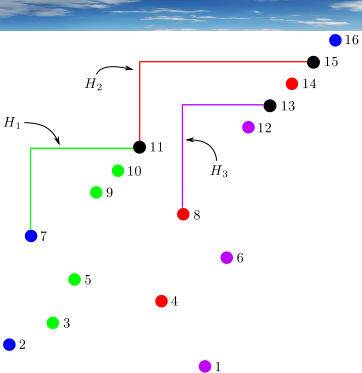
Example 8.8.
Figure 8 shows a valid hook configuration of a permutation in , along with its induced coloring. In this example, there are blue points, green points, red points, and purple points, so . ∎
The following theorem provides a very useful tool for computing fertilities of permutations. It was originally proved in [27], though a clearer and more conceptual proof (which also applies in a much more general setting) appears in [28]. Let denote the Catalan number . Given an integer composition , we write for the product .
Theorem 8.9 (Fertility Formula).
The fertility of a permutation is given by
A simple consequence of the Fertility Formula that will be helpful to keep in mind is that a uniquely sorted permutation (i.e., a permutation with fertility ) must have a unique valid hook configuration.
Let us now turn our attention back to affine permutations. Let us say a set is -periodic if for every integer , we have if and only if . Suppose , and consider the decreasing affine binary plane tree . A left-to-right maximum of is an integer that is larger than every integer appearing to its left in . Let be the left-to-right maxima of . Note that the set of left-to-right maxima of is -periodic. It follows directly from the insertion algorithm that constructs from that is a left child of for every integer . Define the infinite left branch of to be the collection of all the vertices together with all the left edges between these vertices. Now let . By (6), we have . Every left-to-right maximum of is a left-to-right maximum of . Indeed, the numbers appearing before in are the labels (given by ) of the vertices in the left and right subtrees of in , and all of these labels are necessarily smaller than . Furthermore, if denotes the (possibly empty) right subtree of , then is the (finite and possibly empty) permutation appearing between and in the affine permutation . In other words, if , then .
The previous paragraph hints at how to construct each preimage of an affine permutation under . Start with . Choose a nonempty -periodic subset of the set of left-to-right maxima of . This means that there is an integer such that for all . For each index , draw a hook connecting the points and in the plot of . This produces an infinite periodic chain of hooks on the plot of that we call a skyline. Now turn the skyline into an infinite left branch by “unbending” each hook. More precisely, form an infinite tree whose edges are all left edges, and label the vertices of with the elements of so that the vertex with label is the left child of the vertex with label for all . Let be the (finite) permutation whose plot lies underneath (not including the endpoints of ). Because , the permutations and must have the same relative order (i.e., their standardizations are equal) for all . More precisely, is obtained by increasing each of the entries in by . This implies that we can choose permutations for all in such a way that, for each integer , the permutation is obtained by increasing each of the entries in by . Finally, for each , construct the decreasing binary plane tree , and attach it as the right subtree of the vertex of with label . After doing this for all , we obtain a decreasing affine binary plane tree . Let . Our construction guarantees that . It follows from the preceding paragraph that every preimage of under arises uniquely in this way.
Example 8.10.
Let be the affine permutation in with window notation . The plot of is shown on the right in Figure 9. Let be the -periodic subset of the set of left-to-right maxima of given by , , and for all . We have drawn the corresponding hooks on the right side of Figure 9. For example, has southwest endpoint and northeast endpoint , and has southwest endpoint and northeast endpoint . Then , and is the empty permutation. For each integer , the permutation is obtained by increasing each of the entries in by . Let us choose to be the permutation . We are forced to choose to be empty. Our choices of for all are then determined by the condition that is obtained by increasing each of the entries in by . The decreasing affine binary plane tree constructed from these choices is shown on the left in Figure 9. The affine permutation has window notation . Finally, . ∎
The discussion above yields an affine analogue of the Decomposition Lemma from [22, 28]. In order to state it precisely, we fix some notation. Suppose . Let denote the collection of all nonempty -periodic subsets of the set of left-to-right maxima of . The notation comes from the fact that each set in corresponds to a skyline of ; this is the infinite connected chain of hooks , where has southwest endpoint and northeast endpoint . Let us make the convention that the indices of the elements of are chosen so that . For such a set , we let be the index such that for all integers . Also, let be the permutation whose plot lies underneath (not including the endpoints of ). Note that could be the empty permutation , in which case .
Theorem 8.11 (Affine Decomposition Lemma).
For every , we have
If we want to use the Affine Decomposition Lemma to compute the fertility of an affine permutation , then we need to be able to compute the fertilities of the finite permutations appearing in the formula. We can do this using valid hook configurations via the Fertility Formula (Theorem 8.9). We first choose a valid hook configuration for each with . Since each permutation always has the same relative order as , we can copy the hooks from onto the permutations for all and all to produce a periodic configuration of hooks. Together with the hooks in the skyline, this produces a diagram that we call an affine valid hook configuration. When we refer to the skyline of , we mean the skyline of used to construct . Let be the concatenation of the compositions . Let denote the set of affine valid hook configurations of . By combining the Fertility Formula (Theorem 8.9) with the Affine Decomposition Lemma (Theorem 8.11), we obtain the following Affine Fertility Formula.
Theorem 8.12 (Affine Fertility Formula).
For every , we have
Example 8.13.
Preserve the notation from Example 8.10. We have and . Consider the valid hook configuration of that consists of a single hook whose southwest endpoint has height and whose northeast endpoint has height . If we add this valid hook configuration to the image shown on the right of Figure 9, and then repeat it -periodically, we obtain the affine valid hook configuration of shown in Figure 10. Note that is the empty valid hook configuration of the empty permutation. The composition induced by the valid hook configuration is . The composition induced by is the empty composition. The concatenation of and the empty composition is . This corresponds to the fact that, among the points , there are colored green and colored purple in Figure 10. Hence, the affine valid hook configuration of shown in that figure contributes the term to the sum in the Affine Fertility Formula. ∎
Before we proceed, let us pause to collect some observations. Consider an affine valid hook configuration of an affine permutation . The hooks in the skyline of are precisely the hooks that do not lie underneath any other hooks. Also, just as for ordinary valid hook configurations, no hook in passes underneath a point in the plot of . No two hooks in intersect or overlap each other, except when the southwest endpoint of one hook coincides with the northeast endpoint of the other. Every descent top of the plot of must be a southwest endpoint of a hook in . The main difference between ordinary and affine valid hook configurations is that, in the affine setting, not all southwest endpoints of hooks need to be descent tops. Namely, it is possible to have a southwest endpoint of a hook in the skyline of that is not a descent top of the plot of . However, southwest endpoints of hooks that are not in the skyline are required to be descent tops. For our final observation, let be the set corresponding to the skyline of . Suppose that each of the permutations defined above is uniquely sorted. By the Fertility Formula (Theorem 8.9), this implies that each of the compositions has all its parts equal to , so the composition has all its parts equal to .
We now apply the Affine Decomposition Lemma and Affine Fertility Formula to characterize (for even ) which affine permutations attain the maximum in Theorem 8.3. Let us say an affine permutation in is uniquely sorted if its fertility is .
Theorem 8.14.
An affine permutation in is uniquely sorted if and only if it is in the image of and has exactly descents. In particular, there are no uniquely sorted affine permutations in when is odd.
Proof.
First, suppose is uniquely sorted. It follows from the Affine Fertility Formula (Theorem 8.12) that has a unique affine valid hook configuration . Let be the set of left-to-right maxima of corresponding to the skyline of . Let be the hook of with endpoints and , and let be the permutation whose plot lies underneath . Let be the integer such that for all integers . Suppose, by way of contradiction, that there is an integer such that is empty. By periodicity, is empty for all integers . For each integer , delete the hooks and , and replace them with a single hook that has southwest endpoint (the former southwest endpoint of ) and northeast endpoint (the former northeast endpoint of ). This results in a new affine valid hook configuration of , contradicting the uniqueness of . Hence, none of the permutations are empty. It follows that each of the points in the skyline of is a descent top of the plot of . Now let be the number of entries of . The sum counts the entries in and the entries , so it is equal to . It follows from the Affine Decomposition Lemma (Theorem 8.11) that
so each permutation is uniquely sorted. We have shown that each is nonempty, so each is positive. According to Proposition 2.1, each permutation has exactly descents (in particular, is odd). Therefore, the total number of right descents of is .
To prove the converse, assume that is in the image of and has exactly right descents. Because is in the image of , the Affine Fertility Formula (Theorem 8.12) tells us that it has an affine valid hook configuration . Let , , , , and have the same meanings as in the previous paragraph. Let be the set of indices such that the southwest endpoint of is a descent top. Let be the set of indices such that is nonempty. Note that . The hooks in that lie underneath form a valid hook configuration of , so it follows from the Fertility Formula (Theorem 8.9) that is in the image of . If , then since is a nonempty permutation of size in the image of , we have by (2). The number of right descents of is
| (7) |
However, our assumption is that has exactly right descents, so the inequalities in (7) must be equalities. It follows that and for all . By periodicity, we conclude that every southwest endpoint of a hook in is a descent top of the plot of (this is always true of southwest endpoints not in the skyline) and that every permutation for has descents. According to Proposition 2.1, each of the permutations for is uniquely sorted. It follows from the last observation stated immediately before this theorem that the composition has all its parts equal to . Therefore, if we can prove that is the only affine valid hook configuration of , then it will follow from the Affine Fertility Formula that , as desired.
Let be the set of points such that . Let denote the set of descent bottoms of the plot of . Let be the set of northeast endpoints of hooks in . If there were a point , then the hook with northeast endpoint would pass underneath the point , contradicting the properties of an affine valid hook configuration. Therefore, and are disjoint. The assumption that has right descents implies that . Furthermore, every descent top of the plot of is a southwest endpoint of a hook in , so we must have . Since and , we must have . Thus, and form a partition of the set . By periodicity, we find that and form a partition of the set of all points in the plot of .
Recall that our goal is to prove that is the unique affine valid hook configuration of . Suppose instead that there is some other . Let be the set of northeast endpoints of hooks in . We have seen that the southwest endpoints of hooks in are precisely the descent tops of the plot of and that . Applying the same arguments to instead of shows that the set of southwest endpoints of hooks in is also equal to the set of descent tops of the plot of and that . Since , there must be a descent top such that the hook of with southwest endpoint is not equal to the hook of with southwest endpoint . By switching the roles of and if necessary, we may assume that lies underneath (i.e., the northeast endpoint of is higher than that of ). Let be the northeast endpoint of . Let be the set of points lying underneath (not including the endpoints of ), and let . Observe that the leftmost point in is , which is immediately to the right of the southwest endpoint of . This implies that every hook of whose northeast endpoint lies in has its southwest endpoint in . Therefore, is at most the number of descent tops in . The number of descent tops in is the number of hooks of whose endpoints are in , which is also equal to . Since , this implies that . This is our desired contradiction because . ∎
It is not difficult to prove that every affine sylvester class in is infinite when . Therefore, it follows from Theorems 8.4 and 8.14 that the number of uniquely sorted affine permutations in is either or , depending on the parity of . This means that the naïve affine analogue of the fact that uniquely sorted permutations are enumerated by Lassalle’s sequence [29] is not so interesting from an enumerative point of view. However, we can still obtain an interesting enumerative result by considering affine sylvester classes as objects in their own right. Theorem 8.4 tells us that if an affine sylvester class contains a uniquely sorted affine permutation, then all of the affine permutations in that class are uniquely sorted. Hence, we define an affine sylvester class to be uniquely sorted if its elements are uniquely sorted.
Every affine sylvester class contains a unique -avoiding affine permutation, so enumerating uniquely sorted affine sylvester classes is the same as enumerating uniquely sorted -avoiding affine permutations. In the symmetric group setting, -avoiding uniquely sorted permutations were enumerated in [21], where it was shown that they are in bijection with intervals in Tamari lattices. In order to obtain an analogous result in the affine setting, we first need to understand the structure of -avoiding affine permutations.
Given , define to be the affine permutation in given by for all integers . We are going to make use of the injection sending each permutation to the unique affine permutation in that agrees with on (i.e., the affine permutation with window notation ). The direct sum of permutations and is the permutation defined by
Suppose is an integer. It follows from the definition of a valid hook configuration that if is a permutation that has a valid hook configuration, then . Let be the set of -avoiding uniquely sorted permutations such that the unique valid hook configuration of has a hook with southwest endpoint and northeast endpoint . Let be the set of permutations in that can be obtained from a permutation by deleting the last entry . It will be convenient to define to be the empty set.
Now suppose is a -avoiding affine permutation in . Let be the unique affine valid hook configuration of , and let be the set of left-to-right maxima of corresponding to the skyline of . Let , , and be as described above. Assume the indices are chosen so that . Let be the permutation whose plot consists of the points lying underneath together with the southwest endpoint of . Let be the permutation whose plot consists of the points lying underneath together with both endpoints of . Let , , and be the standardizations of , , and , respectively. Let be the size of (so is the size of , and is the size of ). We saw in the proof of Theorem 8.14 that is nonempty and uniquely sorted and that the southwest endpoint of is a descent top. It follows from Proposition 2.1 that has descents. Therefore, has descents. The hooks in that lie on points in the plot of form a valid hook configuration of , so is in the image of by the Fertility Formula (Theorem 8.9). It follows from Proposition 2.1 that is uniquely sorted. Consequently, . Also, is obtained by deleting the entry from , so . Because is in the skyline of , its southwest endpoint is higher up than all points to its left. Since is -avoiding, every point in the plot of appearing to the left of the points in the plot of must also be below all of the points in the plot of . Similarly, every point in the plot of appearing to the right of the points in the plot of must also be above all of the points in the plot of . We deduce that can be written as , where and each is in . Furthermore, there is a unique choice of such that .
Example 8.15.
Consider the -avoiding uniquely sorted affine permutation with window notation . The unique affine valid hook configuration of appears in Figure 11. The hook has endpoints and . The hook has endpoints and . Also, . We have , , and , so , , and . Also, . Similarly, we have , , , , , , and . Then and , so and . The decomposition described above takes the form , where . ∎
The decomposition described above is unique. On the other hand, if we are given positive integers summing to , an integer satisfying , and permutations with for all , then is a uniquely sorted -avoiding affine permutation in . Indeed, each is obtained by deleting the largest entry from a permutation . The unique affine valid hook configuration of is obtained by gluing together the valid hook configurations of , which are essentially the same as the valid hook configurations of , and repeating modulo . It then follows from the Affine Fertility Formula (Theorem 8.12) that the resulting affine permutation is indeed uniquely sorted. Thus, we have the following lemma.
Lemma 8.16.
Every -avoiding uniquely sorted affine permutation in can be written uniquely as , where for all , , and .
An argument similar to the one used to prove Lemma 8.16 yields the next lemma.
Lemma 8.17.
Every -avoiding uniquely sorted permutation in can be written uniquely as , where for all and .
Example 8.18.
The -avoiding uniquely sorted permutation , whose unique valid hook configuration is presented in Figure 12, can be written as . We have and . ∎
Theorem 8.19.
For each , the number of uniquely sorted affine sylvester classes of , which is also the number of -avoiding uniquely sorted affine permutations in , is
Proof.
Let denote the set of -avoiding uniquely sorted permutations in . Let denote the set of -avoiding uniquely sorted affine permutations in . Each uniquely sorted affine sylvester class of contains a unique element of , so we just need to count the elements of . Let
Observe that . It follows immediately from Lemma 8.17 that . This means that . Similarly, it follows from Lemma 8.16 that . Combining these facts, we find that
| (8) |
We know by Proposition 2.1 that when is even. On the other hand, [21, Corollary 6.1] states that
Let . The coefficients of appear as OEIS sequence A000260 [43]; it is stated there that , where satisfies the equation . Thus, . Using Mathematica, one can solve this equation explicitly for and then use that explicit expression to verify that
Therefore, we can use (8) to see that
Now let
According to OEIS entry A107026 [43], the generating function satisfies the equation
In fact, is uniquely determined by the fact that it satisfies this equation and satisfies . Since is another series satisfying this equation and satisfying , we must have . This completes the proof. ∎
Remark 8.20.
As mentioned in Section 2, much of the early work on West’s stack-sorting map developed around the notion of a -stack-sortable permutation and arose from Zeilberger’s [64] theorem that the number of -stack-sortable permutations in is . Our final theorem provides an affine analogue of Zeilberger’s result.
In the next lemma, recall that a left-to-right maximum of a permutation is an entry in that is larger than all entries appearing to its left in .
Lemma 8.21.
Let be a permutation of a set of consecutive integers obtained by concatenating a number with a -avoiding permutation . Then is -avoiding if and only if or is a left-to-right maximum of .
Proof.
If , then certainly is -avoiding. Suppose is a left-to-right maximum of . If there were entries and such that formed a -pattern in , then would form a -pattern in . This cannot happen, so is -avoiding.
Conversely, suppose and is not a left-to-right maximum of . There is an entry that appears to the left of in , so form a -pattern in . ∎
Consider , and let . Suppose is -stack-sortable. Equivalently, is -stack-sortable. Equivalently (by Proposition 8.2), is -avoiding. Let be the left-to-right maxima of . Then . Let us assume the indices are chosen so that . Let . Then by (6). Let be the (possibly empty) right subtree of in , and let . The one-line notation of is . Let . Then each permutation is -avoiding, so each permutation is -stack-sortable (recall that Knuth showed that -stack-sortable permutations are the same as -avoiding permutations). All of the entries in are smaller than because they are labels of vertices lying below in . Furthermore, every entry in is smaller than every entry in since, otherwise, would form a -pattern in . It follows from these observations that for every integer , the entries in form a set of consecutive integers. By Lemma 8.21, the entry is either the smallest entry in or is more than a left-to-right maximum of . Let be the unique integer such that for all , and let be the size of . Finally, let . Since , the assumption that guarantees that . See Example 8.22.
The decomposition of a -stack-sortable affine permutation described in the previous paragraph is reversible. That is to say, is uniquely determined once we choose the integers that sum to , the standardizations of the permutations for , and the integer satisfying . To describe the restrictions on , let be its standardization. Let . Then must be -stack-sortable, and either or is a left-to-right maximum of . If we write for the standardization of , then is a -stack-sortable permutation in .

Example 8.22.
Let , and let be the -stack-sortable affine permutation with window notation . The decreasing affine binary plane tree is depicted in Figure 13. In the above notation, we have , , and . The subtrees are marked in the figure. We have and . Also, and . Notice that for each , the entries in form a set of consecutive integers. We have and . Also, , , and . Observe that is a left-to-right maximum of , while is a left-to-right maximum of . The permutations and are -stack-sortable, so their standardizations and are also -stack-sortable. Finally, .
Suppose we were given that and and that we were handed the standardizations and along with the integer . The standardizations tell us the relative order of for all , and we can begin to reconstruct the set of entries of by using the fact that each such set of entries is a set of consecutive integers (and ). In fact, since and , this determines the entire one-line notation of up to a global shift of the entries. However, there is a unique choice of this global shift that makes the identity hold. Hence, we can reconstruct . ∎
In what follows, we let and denote, respectively, the set of -stack-sortable permutations in and the set of -stack-sortable affine permutations in . For each permutation , let denote the number of left-to-right maxima of . In the above notation, is the number of ways to choose the value of relative to the values of the entries of so that either or is a left-to-right maximum of . The preceding discussion yields the following lemma.
Lemma 8.23.
For , we have
We can now enumerate -stack-sortable affine permutations.
Theorem 8.24.
Let
We have
Proof.
It follows from Lemma 8.23 that
| (9) |
where . If we let , then
| (10) |
As we mentioned before, -stack-sortable permutations have been studied extensively, and luckily for us, Fang [33] has already investigated the generating function . In fact, [33, Equation (5)] provides an equation for a refinement22 2 In Fang’s notation, is . of that keeps track of several additional statistics. By setting most of the variables in that equation equal to , we arrive at the equation
| (11) |
Let us write for . Differentiating each side of (11) with respect to yields
Now put , and set in the previous equation to obtain
Hence,
By (10), we have
Zeilberger’s enumeration of -stack-sortable permutations [64] tells us that
so
Finally, by (9), we have
9. Future Directions
We have initiated the combinatorial and dynamical analysis of Coxeter stack-sorting operators, but it seems we have only grazed the surface. Here, we collect suggestions for future work.
9.1. Other Special Lattice Congruences
There are many special lattice congruences on symmetric groups whose associated Coxeter stack-sorting operators have not been explored. For example, it could be fruitful to investigate more thoroughly the Coxeter stack-sorting operators on arising from Reading’s Cambrian congruences [49]. Recall that these are the same as the -permutree congruences for . One particularly interesting Cambrian congruence from [49] is the bipartite Cambrian congruence, which is obtained by setting , where when is odd and when is even.
9.2. Upward Projection Maps
Suppose is a lattice congruence on the left weak order of a finite Coxeter group . Every congruence class of has a unique maximal element, and we denote by the upward projection map that sends each to the maximal element of the congruence class containing . In analogy with Definition 1.1, we consider the map defined by . The long-term dynamical behavior of can be more complicated than that of because there can be multiple periodic points. It would be interesting to gain an understanding of these new operators, even for specific lattice congruences on symmetric groups.
As an example, consider the sylvester congruence on . For , let be the reverse of . Dukes [31] introduced the map . One can show that for all . In addition, one can show that the identity permutation is the only periodic point of in . Experimental data (checked for ) suggests that the maximum size of a forward orbit of could be for all . By contrast, the maximum size of the forward orbit of an element of under is (see [31]).
Similarly, one can show that for all (recall that is the pop-stack-sorting map). The dynamics of seem interesting. For instance, when , has one fixed point, one periodic orbit of period , one periodic orbit of period , and non-periodic points.
Perhaps one could prove general results, along the same lines as in [26], for the map when is an arbitrary finite irreducible Coxeter group.
9.3. Descents After Coxeter Stack-Sorting
9.4. Stack-Sorting in Type
We believe there is more hidden structure in the type- stack-sorting map . For example, we have the following conjecture.
Conjecture 9.1.
If is odd and , then is even.
In particular, Conjecture 9.1 implies the following weaker conjecture.
Conjecture 9.2.
If is odd and , then .
Recall from Proposition 2.1 that a permutation in is uniquely sorted if and only if it is in the image of and has exactly right descents. In light of Theorem 7.3, one might ask if the elements of with exactly preimage under are the elements in the image of with exactly right descents. This turns out to be false. For example, has exactly preimage under , but it has only right descent.
Question 9.3.
Let be even. Suppose is in the image of and has exactly right descents. Is it necessarily true that ?
Question 9.4.
Let be even. How many elements of in the image of have exactly right descents?
Theorem 7.2 tells us that for all and that there exists such that .
Question 9.5.
How many elements of are such that ?
The sequence of numbers requested in the previous question appears to be new; it begins with the numbers .
In [24], the author gave asymptotic lower and upper bounds for , the average number of iterations of needed to send a permutation in to the identity permutation . Let us similarly define to be the average number of iterations of needed to send an element of to the identity element . We believe the major factors controlling the number of iterations of needed to send permutations to the identity should also be present in type , so we have the following conjecture.
Conjecture 9.6.
We have
9.5. Affine Stack-Sorting
We saw in Section 8 that the affine stack-sorting map shares several of the stack-sorting map’s nice properties. In [24], the author proved a theorem about fertility monotonicity; it states that for all .
Question 9.7.
Is it true that for all ?
In Section 8, we proved affine analogues of the Decomposition Lemma and the Fertility Formula. These are special cases of the results used in [28] to develop a theory of troupes, which are families of binary plane trees that are closely related to the link between the stack-sorting map and free probability theory. It would be very interesting to have a parallel theory of affine troupes, especially if such a theory could connect with free probability theory (or some variant thereof).
10. Acknowledgments
The author thanks Nathan Reading for a helpful conversation. He also thanks the anonymous referees for providing very useful feedback. The author was supported by a Fannie and John Hertz Foundation Fellowship and an NSF Graduate Research Fellowship.
References
- [1] M. Albert and V. Vatter, How many pop-stacks does it take to sort a permutation? Comput. J., (2021).
- [2] D. Albertin, V. Pilaud, and J. Ritter, Removahedral congruences versus permutree congruences. Electron. J. Combin., 28 (2021).
- [3] A. Asinowski, C. Banderier, and B. Hackl, Flip-sort and combinatorial aspects of pop-stack sorting. Discrete Math. Theor. Comput. Sci., 22 (2021).
- [4] A. Asinowski, C. Banderier, S. Billey, B. Hackl, and S. Linusson, Pop-stack sorting and its image: permutations with overlapping runs. Acta. Math. Univ. Comenian., 88 (2019), 395–402.
- [5] D. Avis and M. Newborn. On pop-stacks in series. Util. Math., 19 (1981), 129–140.
- [6] J.-L. Baril, G. Cerbai, C. Khalil, V. Vajnovszki, Catalan and Schröder permutations sortable by two restricted stacks. Inform. Process. Lett., 171 (2021).
- [7] K. Berlow, Restricted stacks as functions. Discrete Math., 344 (2021).
- [8] A. Björner, Orderings of Coxeter groups. In Combinatorics and algebra (Boulder, Colo., 1983), vol. 34 of Contemp. Math., American Mathematical Society, 1984.
- [9] A. Björner and F. Brenti, Combinatorics of Coxeter groups, vol. 231 of Graduate Texts in Mathematics. Springer, 2005.
- [10] M. Bóna, Combinatorics of permutations. CRC Press, 2012.
- [11] M. Bóna, A survey of stack sortable permutations. In 50 Years of Combinatorics, Graph Theory, and Computing (2019), F. Chung, R. Graham, F. Hoffman, R. C. Mullin, L. Hogben, and D. B. West (eds.). CRC Press.
- [12] M. Bóna, A survey of stack-sorting disciplines. Electron. J. Combin., 9 (2003).
- [13] P. Brändén, On linear transformations preserving the Pólya frequency property. Trans. Amer. Math. Soc., 358 (2006), 3697–3716.
- [14] G. Cerbai, Sorting Cayley permutations with pattern-avoiding machines. Australas. J. Combin., 80 (2021).
- [15] G. Cerbai, A. Claesson, and L. Ferrari, Stack sorting with restricted stacks. J. Combin. Theory Ser. A, 173 (2020).
- [16] G. Cerbai, A. Claesson, L. Ferrari, and E. Steingrímsson, Sorting with pattern-avoiding stacks: the -machine. Electron. J. Combin., 27 (2020).
- [17] G. Chatel and V. Pilaud, Cambrian Hopf algebras. Adv. Math., 311 (2017), 598–633.
- [18] A. Claesson and B. Á. Guðmundsson, Enumerating permutations sortable by passes through a pop-stack. Adv. Appl. Math., 108 (2019), 79–96.
- [19] A. Claesson, B. Á. Guðmundsson, and J. Pantone, Counting pop-stacked permutations in polynomial time. arXiv:1908.08910.
- [20] A. Crites, Enumerating pattern avoidance for affine permutations. Electron. J. Combin., 17 (2010).
- [21] C. Defant, Catalan intervals and uniquely sorted permutations. J. Combin. Theory Ser. A, 174 (2020).
- [22] C. Defant, Counting -stack-sortable permutations. J. Combin. Theory Ser. A, 172 (2020).
- [23] C. Defant, Fertilitopes. arXiv:2102.11836.
- [24] C. Defant, Fertility monotonicity and average complexity of the stack-sorting map. European J. Combin., 93 (2021).
- [25] C. Defant, Polyurethane toggles. Electron. J. Combin., 27 (2020).
- [26] C. Defant, Pop-stack-sorting for Coxeter groups. arXiv:2104.02675.
- [27] C. Defant, Postorder preimages. Discrete Math. Theor. Comput. Sci., 19 (2017).
- [28] C. Defant, Troupes, cumulants, and stack-sorting. Adv. Math., 399 (2022).
- [29] C. Defant, M. Engen, and J. A. Miller, Stack-sorting, set partitions, and Lassalle’s sequence. J. Combin. Theory Ser. A, 175 (2020).
- [30] C. Defant and K. Zheng, Stack-sorting with consecutive-pattern-avoiding stacks. Adv. Appl. Math., 128 (2021).
- [31] M. Dukes, Revstack sort, zigzag patterns, descent polynomials of -revstack sortable permutations, and Steingrímsson’s sorting conjecture. Electron. J. Combin., 21 (2014).
- [32] M. Elder and Y. K. Goh, -pop stack sortable permutations and -avoidance. Electron. J. Combin., 28 (2021).
- [33] W. Fang, Fighting fish and two-stack-sortable permutations. Sém. Lothar. Combin., 80B (2018).
- [34] S. Giraudo. Algebraic and combinatorial structures on pairs of twin binary trees. J. Algebra, 360 (2012), 115–157.
- [35] I. Goulden and J. West, Raney paths and a combinatorial relationship between rooted nonseparable planar maps and two-stack-sortable permutations. J. Combin. Theory Ser. A, 75 (1996), 220–242.
- [36] F. Hivert, J.-C. Novelli, and J.-Y. Thibon, The algebra of binary search trees. Theoret. Comput. Sci., 339 (2005), 129–165.
- [37] H. P. Hoang and T. Mütze, Combinatorial generation via permutation languages. II. Lattice congruences. To appear in Israel J. Math., (2021).
- [38] D. E. Knuth, The Art of Computer Programming, vol. 1: Fundamental Algorithms. Addison-Wesley, 1973.
- [39] S. Law and N. Reading. The Hopf algebra of diagonal rectangulations. J. Combin. Theory Ser. A, 119 (2012), 788–824.
- [40] J.-L. Loday. Realization of the Stasheff polytope. Arch. Math. (Basel), 83 (2004), 267–278.
- [41] J.-L. Loday and M. O. Ronco. Hopf algebra of the planar binary trees. Adv. Math., 139 (1998), 293– 309.
- [42] H. Mularczyk, Lattice paths and pattern-avoiding uniquely sorted permutations. Discrete Math. Theor. Comput. Sci., 22 (2021).
- [43] The On-Line Encyclopedia of Integer Sequences, published electronically at http://oeis.org, 2021.
- [44] V. Pilaud. Brick polytopes, lattice quotients, and Hopf algebras. J. Combin. Theory Ser. A, 155 (2018), 418–457.
- [45] V. Pilaud and V. Pons, Permutrees. Algebr. Comb., 1 (2018), 173–224.
- [46] V. Pilaud, V. Pons, and D. Tamayo Jiménez. Permutree sorting. arXiv:2007.07802.
- [47] V. Pilaud and F. Santos. Quotientopes. Bull. Lond. Math. Soc., 51 (2019), 406–420.
- [48] L. Pudwell and R. Smith, Two-stack-sorting with pop stacks. Australas. J. Combin., 74 (2019), 179–195.
- [49] N. Reading, Cambrian lattices. Adv. Math., 205 (2006), 313–353.
- [50] N. Reading. Finite Coxeter groups and the weak order. In Lattice theory: special topics and applications. vol. 2, pages 489–561. Birkhäuser/Springer, 2016.
- [51] N. Reading, Lattice congruences, fans and Hopf algebras. J. Combin. Theory Ser. A, 110 (2005), 237–273.
- [52] N. Reading, Lattice congruences of the weak order. Order, 21 (2004), 315–344.
- [53] N. Reading, Noncrossing arc diagrams and canonical join representations. SIAM J. Discrete Math., 29 (2015), 736–750.
- [54] N. Reading, Sortable elements and Cambrian lattices. Algebra Univ., 56 (2007), 411–437.
- [55] N. Reading and D. Speyer, A Cambrian framework for the oriented cycle. Electron. J. Combin., 22 (2015).
- [56] N. Reading and D. Speyer, Cambrian frameworks for cluster algebras of affine type. Trans. Amer. Math. Soc., 370 (2018), 1429–1468.
- [57] N. Reading and D. Speyer, Combinatorial frameworks for cluster algebras. Int. Math. Res. Not. IMRN, 2016 (2016), 109–173.
- [58] N. Reading and D. Speyer, Sortable elements in infinite Coxeter groups. Trans. Amer. Math. Soc., 363 (2011), 699-761.
- [59] N. Reading and D. Speyer, Sortable elements for quivers with cycles. Electron. J. Combin., 17 (2010).
- [60] M. Singhal, Unimodality of a refinement of Lassalle’s sequence. arXiv:2008.08222.
- [61] H. Úlfarsson, Describing West--stack-sortable permutations with permutation patterns. Sém. Lothar. Combin., 67 (2012).
- [62] P. Ungar, noncollinear points determine at least directions. J. Combin. Theory Ser. A, 33 (1982), 343–347.
- [63] J. West, Permutations with restricted subsequences and stack-sortable permutations, Ph.D. Thesis, MIT, 1990.
- [64] D. Zeilberger, A proof of Julian West’s conjecture that the number of two-stack-sortable permutations of length is . Discrete Math., 102 (1992), 85–93.