Low elements and small inversion sets are in bijection in rank 3 Coxeter groups
Abstract
In this extended abstract we announce a proof that, in a Coxeter group of rank 3, low elements are in bijection with small inversion sets. This gives a partial confirmation of Conjecture 2 in [Dyer, Hohlweg ’16]. That same article provides the main ingredient: the bipodality of the set of small roots is used to propagate information on the vertices of inversion polytopes.
keywords
Infinite Coxeter group, low element, inversion polytope.One of the reasons that Coxeter groups are so well studied, other than their ubiquity, is perhaps their position at the intersection of group theory, combinatorics and geometry. A most impressive example of a result made possible by this confluence is the proof by Brink & Howlett in [1] of the automatic structure of infinite Coxeter groups. Indeed, the combinatorial construction of an automaton recognizing the reduced words of the Coxeter group is based on the notion of small roots which is geometric in nature. In [2], Hohlweg, Nadeau & Williams explore the connection of Garside shadow and low elements with families of automatas recognizing the reduced words of a Coxeter group. These two objects, the latter being an example of the former, were introduced by Dyer & Hohlweg in [3] and were motivated by questions of decidability of the word problem in Braid groups.
In this paper, we focus our study on low elements and specially on Conjecture 2 of [3], where Dyer & Hohlweg ask whether low elements are in bijection with small inversion sets. This conjecture, if true, would give a connection with Shi arrangements and can in fact be formulated as "low elements are in bijection with Shi regions". As Shi arrangements and their regions are extensively studied ([4] or [5] for instance), this could reveal a structure on the set of low elements or, conversely, provide a model for the Shi regions.
In this extended abstract, we announce a proof to this conjecture in the case of rank 3 Coxeter groups. In Section 1, we recall notions on Coxeter groups with emphasis on geometric constructions: root systems, inversion sets, projective picture, and the Tits cone. In the following Section 2 we present the conjecture. Finally, in Section 3, we explain our strategy for the proof in rank 3 before sketching the demonstrations of its main steps.
1 Coxeter groups and geometry: a brief guided tour
In this section we recall notions related to Coxeter groups necessary both for the statement of the conjecture in Section 2 and the sketches of proofs in Section 3.
1.1 Geometric representations and based root systems
Let be a finite dimensional real vector space equipped with a symmetric bilinear form . A simple system in is a set of such that :
- 1.
is positively linearly independent meaning that no line trough is contained in the cone generated by .
- 2.
For all , .
- 3.
For all distinct , .
Let where is the -reflection associated with . Denote by the subgroup of the group of -orthogonal linear maps generated by ; we say that is a Coxeter group and that is a Coxeter system of rank . The length of an element , denoted by , is the minimal length of a product of generators equal to . For all , . When , we say that is a descent of and that is covered by . The transitive reflexive closure of the covering relation is called the right weak order and is denoted by .
We say that is a geometric representation of . When is linearly independent and , we get the . The orbit of under is called the root system and is denoted by (see Figure 1). The pair is called a based root system (as used in [6]). Based root systems enjoy the following usual properties:
- •
The root system is partitioned in positive roots and negative roots .
- •
For , .
In addition, based root systems restrict well to reflection subgroups. Indeed, let , if is the subgroup of generated by -reflections associated to , we set , and to be the roots generating the extreme rays of ; then is a geometric representation of of which is a based root system. Beware: it needs not be a classical representation even when the original representation is.
This restriction property allows to test if a reflection subgroup is finite: it is if and only if where is the isotropic cone of .
1.2 Inversion sets
For the remainder of this paper, we fix a Coxeter system of finite rank. Many of the combinatorial definitions on Coxeter groups have geometric equivalents through inversion sets. We recall below some of their properties (see [7] for details).
Proposition 1.
Let be a group element. The (right) inversion set of is . The inversion set map from to the power set of is an increasing injection. Moreover, is a descent of if and only if for some .

Denote by the set of right geometric descents, or descents for short. We want to draw the reader’s attention on the fact that and that is possible only if is finite, in which case is uniquely defined by . When this occurs, is called the maximal element of . This will be useful later in Lemma 15.
The question of deciding whether a subset of is an inversion set arises naturally. Fortunately, Proposition 2.11 of [8] gives a simple characterization.
Proposition 2.
Let be the root system of a geometrical representation of . A subset of is an inversion set if and only if it is finite and separable: there exists some hyperplane such that is strictly on one side of and is strictly on the other side.
1.3 The projective picture
From now on, we set to be the classical geometric representation of and the corresponding based root system.
In the case of infinite Coxeter groups, can prove challenging to picture: there are infinitely many roots, they are of unbounded norm… Following [6], we may obtain a handy depiction of the root system: the projective picture. To a root we associate a normalized root , where is the affine hyperplane generated by . The normalized roots form the set , as shown in Figure 2. We call projective picture the set seen as embedded in . Since is naturally in bijection with , we will identify with .
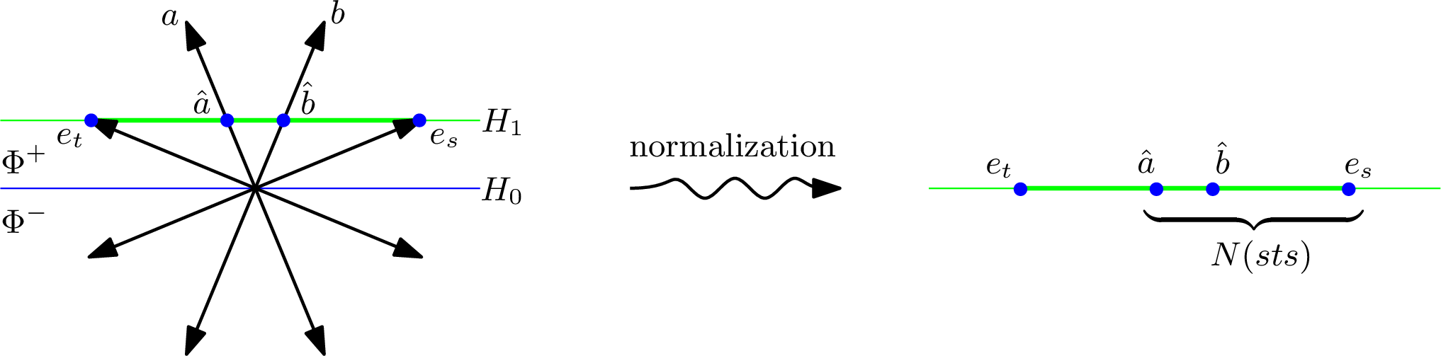
Remark.
Since and , we have , the convex hull of . Because of this, the projective picture is essentially the image of by the canonical projection in the projective space .
More than a simple tool to draw pictures of rank 3 or 4 root systems, the projective picture has several advantages. Because it is a subset of a compact set, has accumulation points which, by [6], are on the isotropic cone (strictly speaking, on ). This circumscribes the treatment of many topological issues to a neighborhood of . In our proofs in Section 3, it will also allow us to simplify the formalism: cones become convex hulls, extreme rays become points, etc. This allows us to translate the inversion set into an "even more" geometric object.
Definition 3.
The inversion polytope of an element in is the convex hull of in . It is denoted by . The set of its vertices is denoted by .
Recall that is separable. This too translates in the projective picture: there exists some affine hyperplane of strictly separating the inversion polytope from its complement in . This imposes that is convex in the sense that (see [8, Lemma 2.10]): and hold the same information.
1.4 The Tits cone
We present here the notion of Tits cone which can be understood as a dual of the root system. This dual point of view will be useful in stating simply the proofs in §3.1 where we examine the interactions of inversion sets and moving separation hyperplanes. We refer to [9] for more details.
Recall that we have fixed of finite rank, which means that is finite dimensional. We denote by the duality bracket. For we set , and . The map is a bijection from the sphere of to the set of closed half-spaces of which is bicontinuous.
Let the set be the fundamental chamber and its closure for the usual topology, then the Tits cone of is . The connected components of are called the Weyl chambers. They are in bijection with via , where acts on by duality. Fix a root and a Weyl chamber . We say that is a wall of if spans . Walls give us yet another way to recognize inversions and descents.
Proposition 4.
For any , if and only if . Moreover is a descent of if and only if and is a wall of .

2 The Dyer-Hohlweg conjecture
In this section, we state the conjecture, briefly explain its connection with Shi regions, and present the notion of bipodality.
Definition 5.
We say that is a small root if for all , there is some such that and . The set of small roots is denoted by .
For , is the small inversion set of . We denote by the set of all small inversion sets.
An element of is a low element if . The set of low elements is denoted by .
Said in the language of the projective picture, where extreme rays of cones become extreme points of convex sets, an element is low if and only if the vertices of its inversion polytope are small roots; that is . Because we already know that the map is injective, the map is injective as well. Is it surjective?
Conjecture 1.
[3, Conjecture 2, Dyer, Hohlweg ’16] The map is a bijection between low elements and small inversion sets.
Let us restate this in terms of Shi regions, that is, the connected components of where is the Tits cone and is the Shi arrangement (this is equivalent to the usual definition, see [10, p.123]). As the Weyl chambers are in bijection with inversion sets, the Shi regions are naturally in bijection with the small inversion sets. Considering this, the question becomes "are low elements in bijection with Shi regions?".
In the same paper where Dyer & Hohlweg introduce the conjecture ([3]), they define the notion of bipodality and prove that the set of small roots is bipodal. This property will be central in the proof in the next section. We illustrate it in Figure 4.

Definition 6.
Let be a line in the projective picture and, as in §1.1, let be the reflection subgroup corresponding to , the roots contained in . We say that the pair is an arrow from to if is a simple root and is not, and denote it . A subset is said to be bipodal if for any arrow , implies .
Theorem 7.
[3, Dyer, Hohlweg ’16, Theorem 4.18] is always bipodal.
3 The result
We are now in position to state our main result – Conjecture 1 holds in rank 3 – and sketch its proof.
Proposition 8.
In rank 3, is surjective.
Strategy.
Recall that an element is low if and only if the vertices of are in . Thus, we can prove this result by exhibiting for any small inversion set an element such that and . Our strategy is as follows:
The most difficult point is to show that the sources form a subset of the descents. We present here a proof in rank 3 and it is the only part of the proof that does not easily extend to higher ranks. We begin by some remarks on the interaction between moving separations hyperplane and inversion polytopes in §3.1. This gives us some tools to prove that is acyclic in §3.2 and to localize the sources of the graph in §3.3.
3.1 Wiggling hyperplanes
As can be seen on Figure 3, the set of separation hyperplanes for is homeomorphic to . This shows, for instance, that if are two separation hyperplanes for , we can continuously move one to the other. In this spirit, we examine in this section some interactions between roots and moving hyperplanes, beginning with a relaxation of the separability condition.
Definition 9.
Let be an element of and its inversion polytope. We say that an affine hyperplane is a weak separation hyperplane for if is on one side of , while its complement is strictly on the other side and does not intersect the normalized isotropic cone.


For finite subsets of , this is equivalent to the regular separability condition: a weak separation hyperplane does not cross the isotropic cone so it is at a strictly positive distance of the roots it does not contain. This gives us a root free envelope (fig. 5(a)) in which we may translate to make it into a strict separation hyperplane (fig. 5(b)). Because the set is bounded, we may actually exit this envelope, as long as we do it "far enough": we can tilt to remove the vertices of (fig. 5(c)). This gives us indications on the descents of an element:
Lemma 10.
Let be an element of , and its inversion polytope. We suppose that is a weak separation hyperplane for containing a face of . Then the vertices of are in .
This lemma expresses a more general idea: because small perturbations of a point in the Coxeter complex correspond to small perturbations of a separation hyperplane, we can choose to enter a chamber through one of its walls.
3.2 is acyclic.
Let be a small inversion set, let us show that we can choose with and , as per the first point of our strategy. Indeed, if it is not the case then remove . Notice that the resulting set of roots is still the inversion set of some and that the small inversion set is unchanged. Repeat. Because the initial is of finite length, this eventually terminates. We obtained the following lemma:
Lemma 11.
Let be a small inversion set. Then there exists some such that and .
We now want to show that every vertex of is accessible from . It is enough to prove that is acyclic and that the sources of (meaning the vertices connected only to outward edges) are a subset of . Indeed, to find a path from to a vertex we just have to follow the following process: if is a source, stop. Else, must be connected by an inward edge to , replace by and iterate. Since there is no cycle, this terminates on a source, which is in .
We now fix the obtained from Lemma 11 for the remainder of this paper. Our next step is to show that the bipodality graph is acyclic. Let us first prove the following useful lemma.
Lemma 12.
We say that a permutation of is a removal order if for all , for some . Let be an edge of with . Then the roots on are removed from to .
Proof.
Notations are defined on Figure 6. Suppose we remove first. Since the remaining roots form an inversion set, it means that a separation hyperplane must cut the line between and and between and : this is absurd. ∎

Remark.
Note that this argument has two consequences. Firstly, an edge of is either an arrow or complete, meaning . Secondly, it means that any removal order determines an orientation on the edges of . Indeed, even if is complete, if is removed first, the remaining roots on must be removed from to . This allows us to define a (directed) removal graph formed of the vertices and edges of oriented by : if is an edge of , we note the corresponding edge in .
We can now restate Lemma 12 as: for any order , is a subgraph of . This will help us to reach our goal for this paragraph:
Proposition 13.
The bipodality graph is acyclic.
Proof.
Because is a subgraph of for any removal order , it is enough to show that is acyclic for some . Let be a separation hyperplane. In the spirit of Lemma 10, we further assume that is generic: it is not parallel to any line through two roots in . We continuously translate through , following its orthogonal line. Because is generic, the roots will traverse one at a time: except at these times, is a separation hyperplane for the remaining roots. Hence, this defines a removal order. Since is only possible if visits before , the related removal graph is acyclic. ∎
3.3 The sources of are descents.
The goal of this section is to prove the following proposition:
Proposition 14.
Assume that . Then every source of the bipodality graph on is a descent.
Let be a source: either it is only connected to outward arrows (case 1), or it is connected to at least one complete edge (case 2). Case 1 is easy: such a source in must be a source in any removal graph. In particular, removal graphs obtained by pushing hyperplanes through polytopes (as in Proposition 13) only have one source, which is the first root they meet and thus must be a descent.
Case 2 is harder. First, notice that a simple root cannot be a source because it always can be removed last, which means it is a sink in some removal graph. The only remaining possibility is dealt with in the following lemma.
Lemma 15.
We suppose that is a Coxeter system of rank 3. Let be the inversion polygon of an element . Let be a complete edge of . If , then .
Proof.
Notice first that because is complete, does not intersect the isotropic cone. If we can prove that is a weak separation line for , from Lemma 10 we get that must be a descent. Let be a separation line for , and (resp. ) the closed half-plane associated to (resp. ) containing . We treat here only the case where is finite, that is, is the inversion set of some . If we can move to without meeting any root, we will have shown that . Using Lemma 10 we define a separation hyperplane for . We then rotate to around their intersection point, in the direction where it does not pass through . If we meet a root during the movement, it must be in (see Figure 7). Up to small perturbations of our movement, we may assume that we meet a unique last root , meaning we enter through the wall associated to . We have and by reversing the movement we can remove it and still be left with an inversion set, so . Since , this means so must be the maximal element and . But there is a simple root on either side of because is not a simple root. This is absurd. The case where is infinite is treated similarly by considering the other side of and interpreting walls as three different elements covering a non neutral element. ∎

4 Final remarks
It can be noted that the proof only requires the bipodality property of the set of small roots and thus can be extended to other bipodal sets. In particular, [3, Conjecture 3] proposes that the set of -small roots (a generalization of small roots) is always bipodal. If this is the case, the proof we have presented here generalizes to -low elements and -small inversion sets. It is our hope that this partial result in rank three could be used as a lemma for higher rank as in [3, Lemma 4.21], through the careful choice of rank 3 reflection subgroups. Finally, considering inversion polytopes by themselves yields another special case: one can show that, when all small roots lie on the edges of the simplex formed by in the projective picture, all small inversion polytopes , , are inversion polytopes. This happens for instance in the so called right-angled case or when no pair of generators in commute.
Acknowledgements.
This work was initiated during an internship under the supervision of Christophe Hohlweg in 2017. The author is grateful to Christophe Hohlweg for tutorship, Nathan Chapelier-Laget for helpful conversations, and Nicolas M. Thiéry for advice on writing.References
- [1] B. Brink and R. Howlett “A finiteness property and an automatic structure for Coxeter groups” In Mathematische Annalen 296.1 Springer, 1993, pp. 179–190 DOI: 10.1007/BF01445101
- [2] C. Hohlweg, P. Nadeau and N. Williams “Automata, reduced words and Garside shadows in Coxeter groups” In Journal of Algebra 457 Elsevier, 2016, pp. 431–456 DOI: 10.1016/j.jalgebra.2016.04.006
- [3] M. Dyer and C. Hohlweg “Small roots, low elements, and the weak order in Coxeter groups” In Advances in Mathematics 301 Elsevier, 2016, pp. 739–784 DOI: 10.1016/j.aim.2016.06.022
- [4] S. Fishel, E. Tzanaki and M. Vazirani “Counting Shi regions with a fixed separating wall” In 23rd International Conference on Formal Power Series and Algebraic Combinatorics (FPSAC 2011), Discrete Math. Theor. Comput. Sci. Proc., AO Assoc. Discrete Math. Theor. Comput. Sci., Nancy, 2011, pp. 351–362
- [5] D. Levear “A bijection for Shi arrangement faces” In Sém. Lothar. Combin. 82B, 2020, pp. Art. 47, 12
- [6] C. Hohlweg, J.-P. L. and V. Ripoll “Asymptotical behaviour of roots of infinite Coxeter groups” In Canadian Journal of Mathematics 66.2 Cambridge University Press, 2014, pp. 323–353 DOI: 10.4153/CJM-2013-024-6
- [7] J. Humphreys “Reflection groups and Coxeter groups” Cambridge university press, 1990 DOI: 10.1017/CBO9780511623646
- [8] C. Hohlweg and J.-P. Labb\’e “On inversion sets and the weak order in Coxeter groups” In European Journal of Combinatorics 55 Elsevier, 2016, pp. 1–19 DOI: 10.1016/j.ejc.2016.01.002
- [9] P. Abramenko and K. Brown “Buildings: theory and applications” Springer Science & Business Media, 2008 DOI: 10.1007/978-0-387-78835-7
- [10] A. Bjorner and F. Brenti “Combinatorics of Coxeter groups” Springer Science & Business Media, 2006 DOI: 10.1007/3-540-27596-7